The metallic winds in dwarf galaxies

Abstract

We present results from models of galactic winds driven by energy injected from nuclear (at the galactic center) and non-nuclear starbursts. The total energy of the starburst is provided by very massive young stellar clusters,which can push the galactic interstellar medium and produce an important outflow. Such outflow can be a well, or partially mixed wind, or a highly metallic wind. We have performed adiabatic 3D N-Body/Smooth Particle Hydrodynamics simulations of galactic winds using the gadget-2 code. The numerical models cover a wide range of parameters, varying the galaxy concentration index, gas fraction of the galactic disk, and radial distance of the starburst. We show that an off-center starburst in dwarf galaxies is the most effective mechanism to produce a significant loss of metals (material from the starburst itself). At the same time a non-nuclear starburst produce a high efficiency of metal loss, in spite of having a moderate to low mass loss rate.

1 Introduction

Dwarf galaxies are a crucial ingredient to understand the evolution of the large scale universe, as well as the formation of larger galaxies. The mass of dwarf galaxies range from $10^{7}$ to $10^{10}$ M$\odot$ and their luminosities from $10^{6}$ to $10^{10}$ L$\odot$ (McConnachie, 2012) making them the basic units in the formation and evolution of the more massive galaxies under the $\Lambda$ Cold Dark Matter scenario. However, the details of how and when this type of galaxies are assembled, and whether they have galactic winds are issues of current debate (Mateo, 1998; Recchi & Hensler, 2013; Recchi, 2014). Dwarf galaxies are characterised by their poor metallicity and low masses. They are subdivided in: dwarf irregulars, which have a significant amount of gas, and thus on-going star formation; dwarf ellipticals, which are gas-poor with an old stellar population; and dwarf spheroidal, which are diffuse and practically without gas. The dwarf irregulars associated with a burst often develop galactic winds, and this can define de metal evolution in this galaxies (Skillman, 1997). Those features can be related to the efficiency of such galaxies to loss mass and metals by galactic winds, basically linking the episodes of star formation or interactions with other galaxies. The research of these outflows is essential to fully understand the evolution of dwarf galaxies, their structural properties, and their chemical enrichment (Veilleux et al., 2005).

The galactic winds, according to their metal content, can be divided into two general categories (Matteucci, 2012): a) ordinary winds, in which the metals produced and ejected by stars are well mixed with the gas of the interstellar medium (ISM). Thus the metallicity of the wind and the ISM are the same. b) Enriched winds, where the metals produced and ejected by the stars are not well mixed with the ISM, i.e. the chemical elements produced in the supernovae explosions are carried out to the intergalactic medium (IGM). In this case the galactic wind has a metallicity higher than that of the ISM. An enriched wind is considered a differential wind if it has different ejection efficiencies of a chemical element to another (e.g. the ejection efficiencies for H and He and for heavier elements (Vader 1986; Recchi et al. 2001, 2008)). The efficiency of ejection of each element may differ due to several factors, most importantly the origin of such chemical elements, since they are produced in different sources that can occur at different locations, and times in the ISM. But there are also other factors that could affect, such as the medium in which the elements mix. For instance, in the case of starbursts, their intensity and location (with respect to the potential well of the galaxy) become relevant. There is a wealth of observational evidence of galactic outflows and winds in dwarfs galaxies (e.g. Israel 1988; Meurer et al. 1992; Martin 1996; Pettini et al. 2001; Westmoquette et al. 2007; Strickland 2007; Matsubayashi et al. 2009; Contursi et al. 2013). Also, recently the metallicity of outflows in dwarf starburst galaxies has been determined (Martin et al., 2002; Ott et al., 2005). At the same time, several authors have presented theoretical models to explain the properties of the winds and their impact in the galaxy evolution, including the chemical analysis of the effect of galactic winds in dwarf galaxies (Yin et al. 2010, 2011), as well as simple chemical models which couple the information of the galactic winds in the development of their codes (De Young & Heckman 1994; Marconi et al. 1994; Lanfranchi & Matteucci 2004, 2007). There have been also hydrodynamic simulations that follow in more detail flows in the galaxy (D’Ercole & Brighenti 1999, Mac Low & Ferrara 1999, hereafter MLF99, Recchi et al. 2001, 2008; Rodríguez-González et al. 2011, hereafter Paper I, Recchi & Hensler 2013, hereafter RH13). Other studies include semi-analytical simulations that aim to explain the effects of galactic winds at cosmological scale, and study the interaction of these winds and the intergalactic medium Bertone et al. 2007; De Lucia et al. 2014). These type of studies usually adopt galactic winds with little detail of their evolution, focusing on the moment when the material is uncoupled from the galaxy, and generally do not relate the properties of the wind with other properties of the galaxy, or they simply assume that the galactic wind is proportional to the rate of star formation. Other authors analyze effects of galactic winds in the intracluster medium, making large-scale simulations and using observations of galaxy clusters (such as Höller et al., 2014). In these models, efficiencies of material ejection are averaged given the baryonic mass of the galaxy. An objective of this paper is the study of galactic winds in different host galaxies, varying the properties of the starburst that causes the wind (including the location of the outbreak in the disk of the galaxy). The results can provide better estimates for the efficiencies of ejection of gas mass and metals, thus yielding valuable information to improve the input for large-scale simulations.

In the present paper we have analyze and compare the efficiencies of ejection of pristine gas and of metal rich material in cases where the starburst occurs at the center and off-center of the galactic disk, exploring different values of the concentration parameter of dwarf galaxies, and gas fraction of the galactic disk. Our goal is to understand how the ejection of pristine and enriched gas evolve, and explain the low metallicity observed in these galaxies, as well as the metal content in the IGM. This paper is organized as follows: In Section 2 we describe the ingredients considered in our galactic models, the framework to produce the winds is explained in Section 3. The results are presented in Section 5 and our conclusions in Section 6.

2 Numerical ingredients of the galaxy

The density profiles of dark matter halos are not well constrained for dwarf galaxies, in order to model their mass distribution we used a Hernquist profile (Hernquist 1990).

$$\rho_{\mathrm{h}}(r)=\frac{M_{\mathrm{dm}}}{2\pi}\frac{a}{r(r+a)^{3}},$$ (1)

where $r$ is the radial distance, and $M_{\mathrm{dm}}$ is the dark matter mass. This profile coincides well at the inner parts of the galaxy with the Navarro, Frenk, & White (1996) fitting formula, but declines faster in the outer parts. The total mass converges in the Hernquist profile, allowing the construction of isolated halos without the need of an ad-hoc truncation. The $a$ parameter is related to the scale radius $r_{\mathrm{s}}$ of the NFW profile by $a=r_{\mathrm{s}}\sqrt{2[ln(1+c)]-c/(1+c)}$, where $c=r_{\mathrm{200}}/r_{\mathrm{s}}$ is a ‘concentration index’, $r_{\mathrm{200}}$ is the radius at which the enclosed dark matter mean density is 200 times the critical value (where the critical density is $\rho_{\mathrm{crit}}=3H^{2}/8\pi G$, see Navarro, Frenk, & White (1996), and Springel et al. (2005). We chosen different concentration indices, c, in the range of the dwarf galaxies, $5<c<15$. The circular velocity of our models is given by,

$$v_{\mathrm{c}}(r_{\mathrm{200}})=10\,\mathrm{H_{0}}\,r_{\mathrm{200}},$$ (2)

where H₀ is the Hubble constant.

As in Paper I , we modelled gas and star disk components ($M_{\mathrm{g}}$ and $M_{*}$, respectively) with an exponential surface density profile (in the radial direction of the galactic disk, $R$) with length-scale $R_{0}$,

$$\Sigma_{\mathrm{g}}(R)=\frac{M_{\mathrm{g}}}{2\pi R_{0}^{2}}\exp(-R/R_{0}),$$ (3)

$$\Sigma_{\mathrm{*}}(R)=\frac{M_{\mathrm{*}}}{2\pi R_{0}^{2}}\exp(-R/R_{0}),$$ (4)

One can obtain the disk mass $M_{\mathrm{d}}=M_{\mathrm{g}}+M_{*}=m_{\mathrm{d}}M_{\mathrm{tot}}$), where $m_{\mathrm{d}}$ is a dimensionless parameter (fixed in this work to $m_{\mathrm{d}}=0.041$), and $M_{\mathrm{tot}}$ is the total mass of the galaxy, including the dark matter halo (i.e. $M_{\mathrm{tot}}=M_{\mathrm{d}}+M_{\mathrm{h}}$, where $M_{\mathrm{h}}$ is the mass of the halo).

The vertical mass distribution of the stars in the disk is specified by the profile of an isothermal slab with a constant scale height $H$. The 3D stellar density in the disk is hence given by,

$$\rho_{*}(R,z)=\frac{M_{*}}{4\pi\,H\,R_{0}^{2}}{\rm sech}^{2}\left(\frac{z}{2H}\right)\exp\left(-\frac{R}{R_{0}}\right).$$ (5)

When constructing the galactic models, we assumed that the gas distribution is isothermal and the vertical structure of the gas disk is in hydrostatic equilibrium:

$$\frac{\partial\rho_{\mathrm{g}}}{\partial z}=-\frac{\rho^{2}_{\mathrm{g}}}{P}\frac{\partial\Phi_{\mathrm{T}}}{\partial z},$$ (6)

where $\Phi_{\mathrm{T}}=\Phi_{\mathrm{h}}+\Phi_{\mathrm{d}}$ is the total gravitational potential ($\Phi_{\mathrm{h}}$ and $\Phi_{\mathrm{d}}$ are the halo and disk gravitational potentials, respectively). If one disregards the self-gravity of the gas the above equation simplifies, and can be integrated to a closed solution. However, a more realistic model requires to include the gravity from all the components, and the inclusion of thermal and rotational support, which can only be done numerically (for a thorough study see Vorobyov et al., 2012). In our models we start with a gaseous disk at a temperature of $1000$ K, and an initial guess for the density value at the midplane ($z=0$). For a given $\Phi_{\mathrm{T}}$, the solution of this equation is constrained by the condition

$$\Sigma_{\mathrm{g}}(R)=\int\rho_{\mathrm{g}}(R,z)dz\,,$$ (7)

where $\Sigma_{\mathrm{g}}(R)$ is the surface gaseous mass density (see also Equation 3). One can obtain the vertical distribution by integrating Equation (6) at a given radius, adjusting the local density in an iterative process until the desired surface density (Equation 3) is recovered. This process is repeated for different radii in order to obtain an axisymmetric gas density distribution. With this initial conditions the galaxy models are evolved for an additional 10 Myr before the starbursts are imposed.

2.1 Numerical models

We constructed two galaxies: G1 and G2 with a gas mass of 1.4 $\times$10⁸ M_⊙ and 4.7 $\times$10⁸ M_⊙, respectively, see Table 1 (they correspond to models G4 and G7 in Paper I). We use the Smooth Particles Hydrodynamics (SPH) code gadget-2 to run a set of adiabatic numerical simulations for dwarf galaxies with the purpose to study the effects of the: concentration index (c), gas mass fraction (f_g), the location of the starburst, nuclear and non-nuclear. Nuclear starbursts are imposed at the galactic center, while non-nuclear starbursts are placed at a galactocentric distance $R$ along the $x$-axis, but remaining at the mid-plane of the galaxy ($z=0$). We consider 3 mechanical luminosities (L_m) for the starburst for each of galaxy. L_m=3, 15 and 75 $\times 10^{39}$ erg s^-1 for a host galaxy as G1, L_m=10, 50 and 250 $\times 10^{39}$ erg s^-1 for a host galaxy as G2. That is, the mass of the starbursts are 1.0 $\times$10⁵, 5.0 $\times$10⁵ and 2.5 $\times$10⁶M_⊙ for a galaxy G1, and 3.3 $\times$10⁵, 1.6 $\times$10⁶ and 8.3 $\times$10⁶M_⊙ for a galaxy G2, following a Salpeter initial mass function (Salpeter 1955). In all the cases, the feedback radius (size of the starbust) is $50$ pc. The energy input by the starburst is imposed instantaneously, in a single time-step of the simulation due to the fact that such time-step is of the same order, $1\times 10^{-5}~{}\mathrm{Gyr}$ . The total energy injected was calculated integrating the L_m over the cluster lifetime $40~{}\mathrm{Myr}$, (it was described in Paper I.) In Paper I both cases, adiabatic and radiative were considered, and the results showed that (for such energetic starbursts) it was easier to lose enriched wind material than pristine ISM, regardless of the inclusion of radiative loses. Thus, in order to keep the free parameters to a minimum in the present paper we only consider the adiabatic case. In the table we show the different concentration indices modeled for both galaxies, with a greater $c$ the galaxy is more compact, and with a smaller $c$ the galaxy is more disperse, as shown in Figure 1, where we plotted the density projection of the initial condition with different concentration index for a same gas fraction (f_g=0.35). This effect of galactic mass distribution is also reflected in the value of the scale radius of the galaxy (R₀) for a given $c$,with a decreasing R₀ as $c$ increases (Table 1). We also generated simulations in which $c$ is fixed (taking $c$=9), and the variable parameter is the gas fraction. The f_g describes the relative content of gas in the disk, the rest of the mass is in stars. The variation of fraction of gas is not reflected in the R₀ as in the case of c, because the gas content changes, but the density remains equal. Finally, to analyze the impact of the starburst at different distances from the center of the galaxy (taking $c$=9 and f_g=0.35), we tested a set of simulations with the starburst located a galactocentric distance of R = R₀. All the numerical simulations in this work were built with three types of particles, $10^{5}$ for the disk, $10^{5}$ for the halo, and $5\times 10^{5}$ gas particles. This is factor of $\sim 5$ higher resolution than in Paper I. In addition, for this study, we performed tests with an order of magnitude less and more particles (for the three types), finding that although more detail is seen in the high resolution runs, the efficiencies obtained do not vary considerably compared with the nominal resolution ones.

Table 1: The galactic models

Galaxy	c	Mg	Mh	Vc (r200)	H	R0
Model		(M⊙)	(M⊙)	(km s-1)	(kpc)	(kpc)
G1	$5$	$1.4\times 10^{8}$	$9.4\times 10^{9}$	$34.3$	$0.118$	$0.76$
G1	$9$	$1.4\times 10^{8}$	$9.4\times 10^{9}$	$34.3$	$0.118$	$0.58$
G1	$15$	$1.4\times 10^{8}$	$9.4\times 10^{9}$	$34.3$	$0.118$	$0.45$
G2	$5$	$4.7\times 10^{8}$	$3.2\times 10^{10}$	$51.9$	$0.178$	$1.16$
G2	$9$	$4.7\times 10^{8}$	$3.2\times 10^{10}$	$51.9$	$0.178$	$0.88$
G2	$15$	$4.7\times 10^{8}$	$3.2\times 10^{10}$	$51.9$	$0.178$	$0.68$

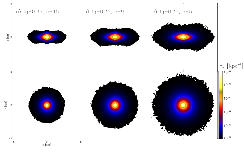
Figure 1: Density projection of the initial condition for the G1 galaxy with the same gas fraction, f_g=0.35, and with different concentration index: a) $c$=15, b) $c$=9, c) $c$=5. Top panels: xz-plane (y=0), taking a slice of the simulation box with a width of 0.2kpc. Bottom panels: yz-plane (x=0), taking a slice of the simulation box with a width of 0.2kpc.

3 Metal rich galactic winds.

The most used outflow rate is the well mixed galactic winds, it represent the case where the mixing between the winds and the ISM is efficient. This result in a uniform metallicity in the galactic wind and the host galaxy (Matteucci, 2012, and references therein). The amount of gas and chemical species as a function of the lifetime of an isolated galaxy, considering instantaneous recycling approximation (Matteucci, 2012) are given by,

$$\frac{dM_{\mathrm{gas}}(t)}{dt}=-(1-R)\psi(t)+f(t)-w(t),$$ (8)

and

$$\frac{d[Z_{i}(t)M_{\mathrm{gas}}(t)]}{dt} = -(1-R)\psi(t)Z_{i}(t)$$ (9)

$$+(1-R_{\mathrm{ms}})\psi(t)y_{i,\mathrm{ms}}$$

$$+(1-R_{\mathrm{lims}})\psi(t)y_{i,\mathrm{lims}}$$

$$+Z^{\mathrm{f}}_{i}f(t)-Z^{\mathrm{w}}_{i}(t)w(t)\,,$$

where $M_{\mathrm{gas}}$ is the gas mass, $w(t)$ the mass outflow from the galactic potential, $\psi(t)$ is the star formation rate, $Z_{i}(t)$ is the time dependent ISM metallicity for the $ith$ source, $y_{i,\mathrm{ms}}$ is the corresponding stellar yield from massive stars ($=\int^{M_{\mathrm{up}}}_{\mathrm{8{\rm M}_{\odot}}}mp_{i}(m)\phi(m)dm/(1-R_{\mathrm{ms}})$), $y_{i,\mathrm{lims}}$ is the stellar yield of low and intermediate mass stars $[=\int^{8{\rm M}_{\odot}}_{\mathrm{M_{\mathrm{low}}}}mp_{i}(m)\phi(m)dm/(1-R_{\mathrm{lims}})]$. The mass fraction returned to the ISM is $R_{\mathrm{ms}}=\int^{M_{\mathrm{up}}}_{\mathrm{8{\rm M}_{\odot}}}(m-m_{r})\phi(m)dm$, while $R_{\mathrm{lims}}=\int^{8{\rm M}_{\odot}}_{\mathrm{M_{\mathrm{low}}}}(m-m_{r})\phi(m)dm$. $R$ is the sum of $R_{\mathrm{ms}}$ and $R_{\mathrm{lims}}$. $M_{\mathrm{low}}$ and $M_{\mathrm{up}}$ are the lower and upper limits of the initial mass function, $\phi(m)$. We used M${}_{\mathrm{low}}=1~{}M_{\odot}$ and M${}_{\mathrm{up}}=100~{}M_{\odot}$ for the mechanical energy calculations.

The term $Z^{\mathrm{w}}_{i}(t)w(t)$ of Equation 9 assumes that the interstellar medium of the host galaxy is well mixed, at least locally (in the starburst region).

In the starburst region the superwind contains the metals produced and ejected by the stars via supernova (SN) explosions, and stellar winds (in main and post-main sequences).

There are several mechanisms that came into play to produce, or inhibit the production of a well mixed wind. For instance, the process of mixing of the metals (formed in the star formation event) with the interstellar medium of the galaxy requires a very long diffusion time. Such diffusion time is around 10⁵ and 10¹⁴ yr for the ionised and molecular regions, respectively (see Tenorio-Tagle, 1996, and references therein). Tenorio-Tagle (1996) presented a model based on the galactic fountains that are able to push hot gas injected by the massive stars from the galactic disk out to the galactic halo. In his model the galactic fountain is made up of metal rich clumps that travel through the halo of the galaxy and fall back to different regions of the galactic disk. As a result the metals are well distributed in the galaxy, mixing with the local interstellar medium and enhancing the process of contamination. However, as pointed out by Recchi et al. (2001), it is necessary to consider that in these models the cooling of the rich clumps could be very important to establish the time in which the metals diffuse, given that it affects its fall back the galactic disk. In other words, the process of mixing is dependent of the cooling by metals and hence the heating efficiency adopted for SNs also it should be taken into account. Additionally, tidal stripping can produce outflows that are inherently well mixed. At the same time, a star formation event with only a few massive stars can increase the metallicity locally, without being able to affect the ISM in the entire host galaxy.

MLF99 and several more recent papers (e.g. Paper I) study the efficiency at which metal rich material is lost by dwarf galaxies with an important star formation event. The general conclusion is that the efficiency of ejection of the metal rich material from the starburst (metal injection efficiency in short, $\xi_{\mathrm{z}}$) is not tied to the total mass ejection efficiency ($\xi_{\mathrm{m}}$). As a result, many models produce a partially mixed galactic wind, in which both the metals produced in the wind, and the pristine ISM material contribute to the galactic outflow.

Using the same definitions of Paper I, the mass ejection efficiency is given by

$$\xi_{\mathrm{m}}=\frac{M_{\mathrm{ej}}}{M_{\mathrm{gas}}},$$ (10)

where M_ej is the gas mass of the galaxy ejected (unbound) and M_gas is the total gas mass.

And the metal ejection efficiency is

$$\xi_{\mathrm{z}}=\frac{M_{\mathrm{c,ej}}}{M_{\mathrm{c}}},$$ (11)

where M_c is the total mass injected via stellar winds and supernova remnants inside the radius of feedback, R_c, and M_c,ej is the mass ejected (unbound) that originated in the starburst. In the present paper, To obtain M_ej from the simulations, we consider their position and velocity. If their velocity is greater than the escape velocity at their location; and if they lie outside a cylindrical region of radius $20$ kpc and $40$ kpc in height, at the center of the galaxy ; they are considered as mass that is effectively lost form the galaxy (see also D’Ercole & Brighenti, 1999).

Assuming a thermal wind driven by an instantaneous starburst event, the galactic wind is a function of the mass and metal ejection efficiencies at the time that the starburst occurs. We propose to use the average mass lost rate as function of mass and metal efficiency as:

$$w(t)=\begin{cases}&\rm{if}\;\;t\;\;\rm{is~{}not~{}within~{}~{}}\Delta t_{\mathrm{lf}}~{}:\\ &0,\\ &\\ &\rm{if}\;\;t\;\;\rm{is~{}within~{}~{}}\Delta t_{\mathrm{lf}}~{}:\\ &\xi_{\mathrm{m}}\frac{M_{\mathrm{gas}}}{\Delta t_{\mathrm{lf}}}+\xi_{\mathrm{z}}\frac{M_{\mathrm{c}}}{\Delta t_{\mathrm{lf}}},\\ \end{cases}$$ (12)

where $\Delta t_{\mathrm{lf}}$ is the lifetime of the massive stars, which is around $10^{7}$ yr).

This way, one can modify the chemical evolution expression in Equation 9 to include the metal ejection efficiency in favour of the mass outflow function $w(t)$. For instance, we can replace the $Z_{\mathrm{i}}^{\mathrm{w}}w(t)$ term in Equation 9, for $(1-R_{\mathrm{ms}})\,\xi_{\mathrm{z}}\,\psi(t)y_{i,\mathrm{ms}}$ if $t$ is within $\Delta t$.

4 Previous works

MLF99 studied the effect of a starburst placed at the center of dwarf galaxies with gas masses between 10⁶ - 10⁹M_⊙. They found that the galaxies with masses of 10⁶M_⊙ have a high efficiency of gas ejection, which is mostly independent from the energy of the starburst (mechanical luminosity, L_m). If the galaxy mass is $\leq$ 10⁸M_⊙ the efficiency of gas ejection is relatively low and still dependent on L_m, while for 10⁹M_⊙ the efficiency is almost null. In the case of the metal ejection efficiency (the efficiency to loose the metal rich material from the starburst) for galaxies with $\leq$10⁸M_⊙ is close to unity and does not depend on L_m, whereas for 10⁹M_⊙ depends significantly on L_m. That is, the metals produced in the starburst escape more easily from the galaxy that the pristine gas (H and He, see tables 2 and 3 of MLF99).

STT01 consider the same range of gas mass of the galaxies that MLF99. They studied the expulsion of gas and its relation to the degree of flatness/roundness of the galaxy, and whether the ejection is in the same direction as its axis of rotation. They also take into account the pressure of the IGM and the existence of gaseous halos. They conclude that the super-bubbles in flat galaxies with rotation, tend to break out from the disk and expel their metal content with only a small amount of pristine ISM gas (the cases of MLF99, fall into these type of galaxies, with low pressure of the IGM). To eject the contents of super-bubbles in spherical galaxies a starburst 3 times more energetic is required in comparison to a flat galaxy (see figure 3 of STT01).

Fragile et al. (2004) (hereafter F04) modeled disk galaxies with masses of 10⁹M_⊙ and one of 10⁸M_⊙, with discrete events of supernovae (SNe) distributed over a fraction of the galactic disk (and one off-centered model). Comparing their models 1 and 2 (same parameters, but in model 1 the SN explosions are all placed at the galactic center, while in model 2 all are placed at the same point off-center). They found that the metal efficiency ejection is higher when the SNe are concentrated in the center (see Section 5 for a comparison with our results).

In Paper I, a wide range of galactic masses was explored (M_g = 6$\times$10⁶ - 10¹¹M_⊙) and central starburst masses (M_SB = 10² - 10⁷M_⊙). The results are in good agreement with those of previous studies, metal efficiency ejection and gas decrease as the mass of the galaxy increases. It is also shown that the values of efficiencies are higher for the more massive bursts (high L_m). Due to the larger mass range of galaxies and starbursts, a model that makes the transition between regimes of low and high efficiencies of ejection was included: M_SB = 3$\times$10⁴M_⊙ and M_g = 3$\times$10⁷M_⊙ (for more details see figures 2 to 5 of Paper I). In Paper I the variation in location of of the starburst for different models was considered, finding that the relation of the ejection efficiency with distance from the radius of the starburst is not monotonic. For the most massive galaxies the fraction of unbound pristine gas was less than 25 percent, while the less massive galaxies lose virtually all their gas content. For the enriched material a large escape fraction is seen in the less massive galaxies, in contrast with the less energetic starbursts, in which most of the metal content is retained, the results are qualitatively consistent with those obtained by MLF99.

RH13 made a similar study to STT01 for galaxies with masses between 10⁷ - 10⁹M_⊙, analyzing the ejection efficiencies varying the mass distribution of the host galaxy. As STT01, they concluded that the ejection of enriched gas on a flat galaxy is higher than on a spherical, while the fate of the pristine gas is relatively independent of the geometry of the galaxy. They also confirm that metal and gas efficiencies ejection are strongly dependent on the galactic mass. Thus, smaller galaxies develop larger flows and the fraction of metals and gas ejected tend to be larger (see table 2 of RH13). In addition, they found that the fate of pristine gas and of newly produced metals are strongly dependent on the mass of the galaxy.

5 Results and discussion

We computed the fraction of total mass and metal rich material (produced in the starburst) that is effectively lost in all the models. After the starburst occurs, the mass and metal ejection efficiencies increase, and after a few tenths of $\mathrm{Gyr}$ they saturate.

In what follows we discuss the effects of the concentration index, the disk gas fraction, and the location of the starburst. The efficiencies were calculated in all cases after an integration time of $t=1~{}\mathrm{Gyr}$ (i.e. $990~{}\mathrm{Myr}$ after the injection of the starburst).

5.1 The concentration index effects

Figure 2 shows the effect of the concentration index in the G1 galaxy after an integration time of $t=0.1~{}\mathrm{Gyr}$ (the starburst occurs at $t=0.01~{}\mathrm{Gyr}$, at the center of the galaxy). In this Figure, it can be noted that more ISM mass (white arrows), and also more metals (green arrows) escape in the models where the concentration of the galaxy is smaller (upper panels). This is due to the fact that the galaxy is less dense for a smaller $c$, and thus it is easier for the energy produced by supernova explosions to break out the bubbles, emptying their content (metal rich) into the IGM, carrying in some cases a significant fraction of pristine ISM along.

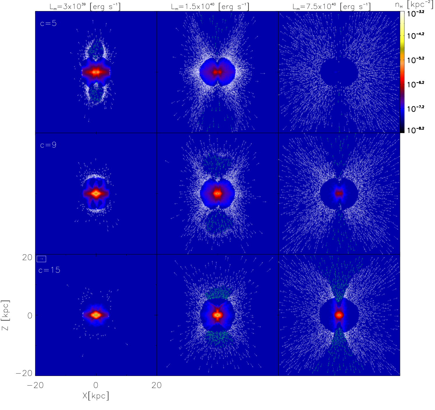
Figure 2: Density cut of the G1 galaxy, xz-plane (y=0), at $t=0.1~{}\mathrm{Gyr}$ (the slice has a thickness of $0.2~{}\mathrm{kpc}$). The star formation event is nuclear (at R=0). The arrows depict the velocity field of particles unbound from the potential well of the galaxy, the white arrows represent the pristine gas mass and the green ones the metals, for visual purposes we plotted only 20% of the arrows. In this figure we show simulations with the same gas fraction, f_g=0.35, with different concentration index, top row: $c$=5, middle row: $c$=9, bottom row: $c$=15; and mechanical luminosities, left column: L_m=3, middle column: L_m=15, and right column: L_m=75 (units: $\times 10^{39}$ erg s^-1).

The least efficient model in mass and metals loss it is that with a larger $c$ and a smaller L_m (bottom left panel), and the most efficient has a smaller $c$ and a larger L_m (upper right panel). This can be confirmed in the top panels of Tables 2 and 3, where we list the mass and metals ejection efficiencies for all the models where the starburst occur at the center of the galaxy.

In Table 2 (top) we show the values of the mass ejection efficiency as a function of $c$ and L_m for both galaxies, with a nuclear starburst. As described for G1 in Figure 2, it is noted that with a lower $c$ and a greater L_m, higher efficiencies are achieved. The G2 galaxy has a mass ejection efficiency low with respect to G1. The reason is that despite that G2 has more energetic starbursts, it is also is more massive, and does not allow at the super-bubbles to break as easily as in G1. Similarly, in Table 3 (top box) we present the values of metal ejection efficiencies, where it can be seen the same trend that that the models with smaller $c$ and larger L_m are very efficient to launch the metals out of the galaxy.

In Figure 3 we show the G1 galaxy with the same parameters of Figure 2, only that in this case the starburst is non-nuclear off the galactic center, and the values of the mass ejection efficiency and metal ejection efficiency are in the Tables 2 to 5 (top boxes), respectively. If we compare the efficiencies of loss of mass and of metals between nuclear and non-nuclear starbursts, we can see that there is not much difference, although in general it is easier to lose mass gas in the models with non-nuclear starburst, the metal loosing efficiencies are rather similar.

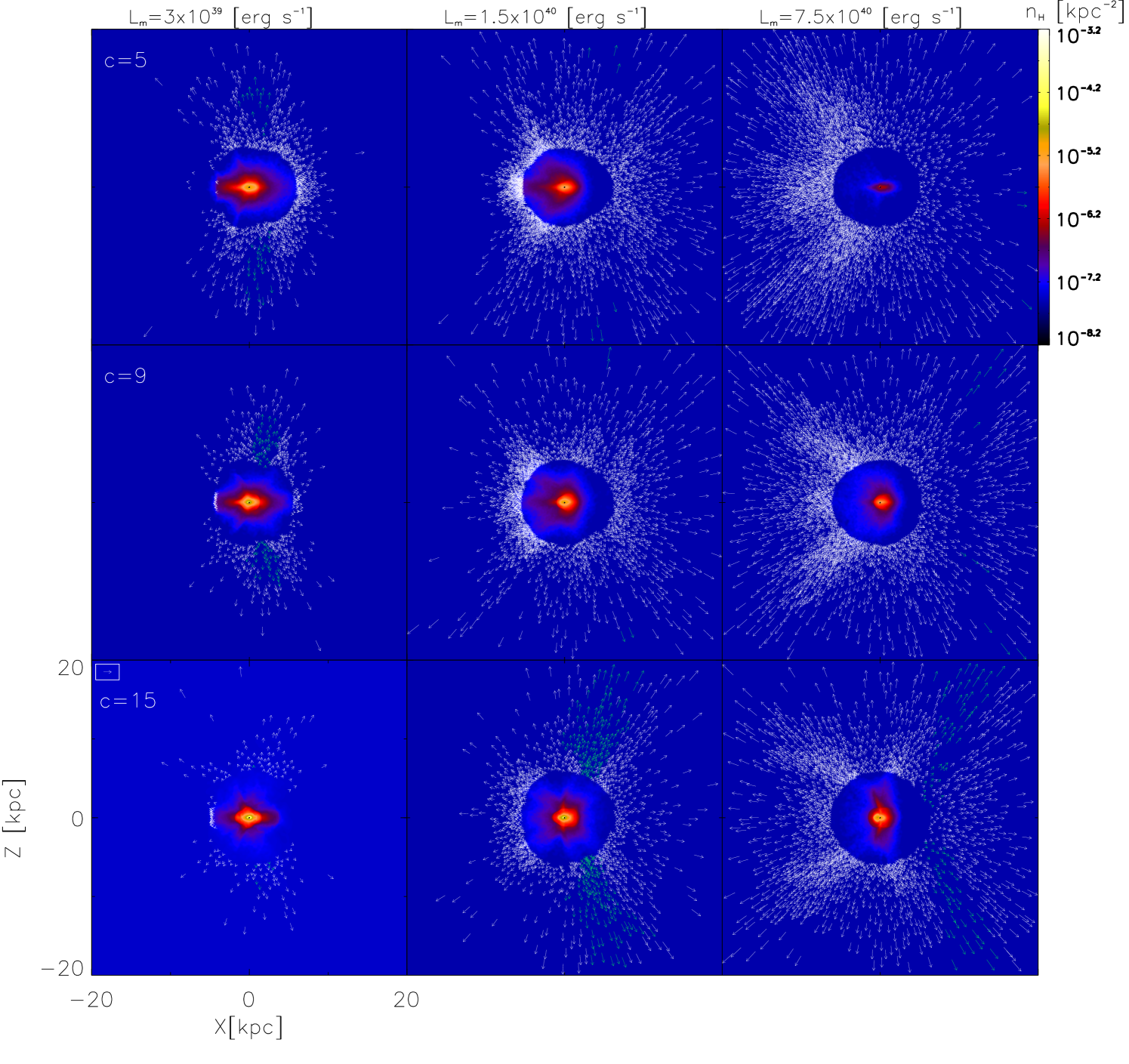
Figure 3: Same as in Figure 2, but for a non-nuclear a star formation event (at R=R₀).

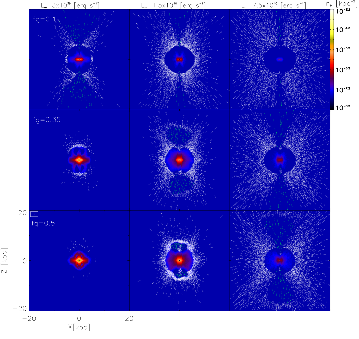
Figure 4: Density cut of the G1 galaxy, xz-plane (y=0), at $t=0.1~{}\mathrm{Gyr}$ (the slice has a thickness of $0.2~{}\mathrm{kpc}$). The star formation event is nuclear (at R=0). The arrows edit1depict the velocity field of particles unbound from the potential well of the galaxy, the white arrows represent the pristine gas mass and the green ones the metals, for visual purposes we plotted only 20% of the arrows. In this figure we show the simulations with different gas fraction, top row: f_g=0.1, middle row: f_g=0.35, bottom row: f_g=0.5 and with the same concentration index, $c$=9; vs mechanical luminosity, left column: L_m=3, middle column: L_m=15, and right column: L_m=75 (units: $\times 10^{39}$ erg s^-1).

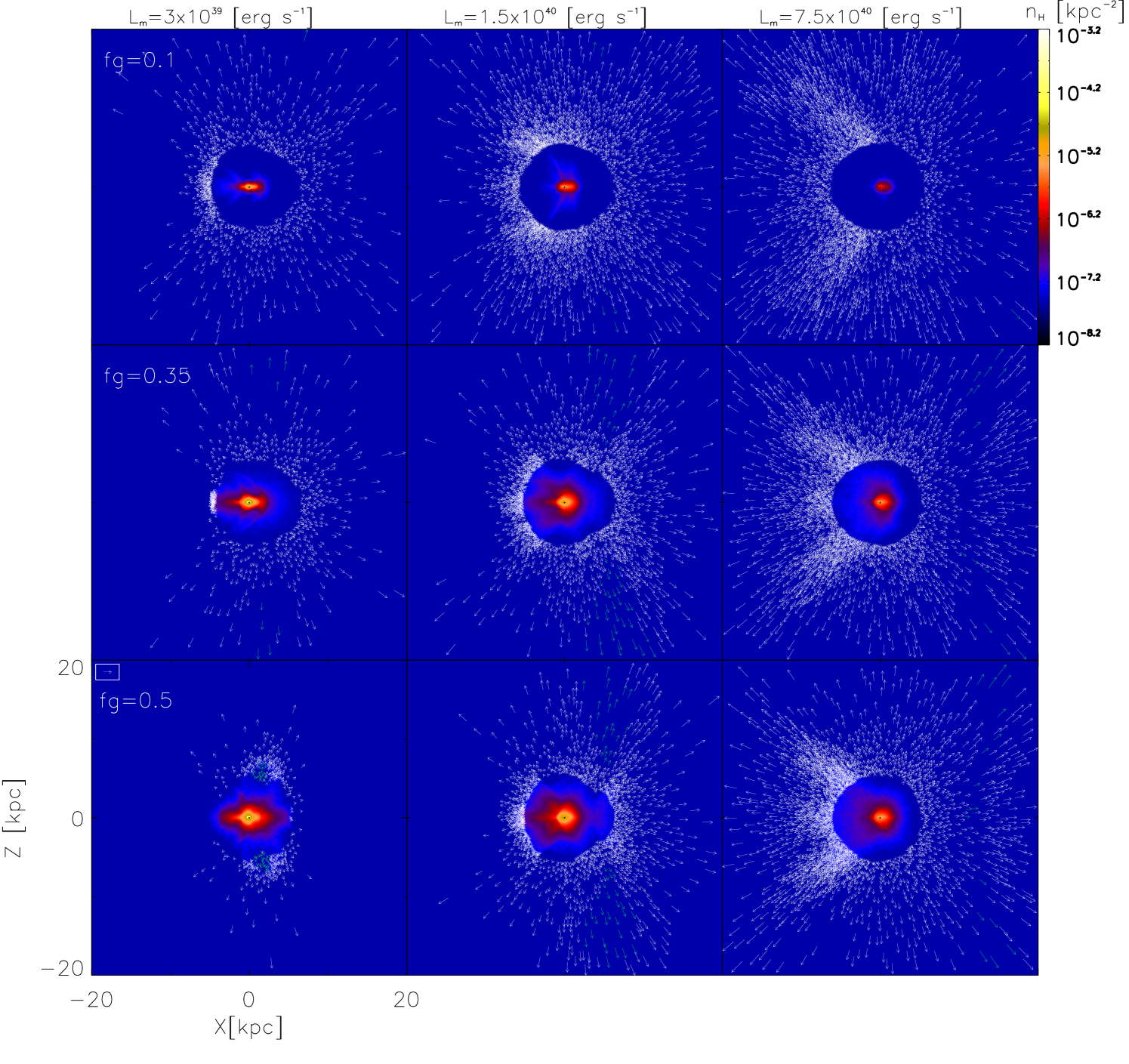
Figure 5: Same as Figure 4, but for a non-nuclear star formation event (at R=R₀).

Table 2: Mass ejection efficiency of nuclear starbursts

	Lm ($\times 10^{39}$ erg s-1)			Lm ($\times 10^{39}$ erg s-1)
	$3$	$15$	$75$	$10$	$50$	$250$
c	G1 ($f_{\mathrm{g}}=0.35$)			G2 ($f_{\mathrm{g}}=0.35$)
$5$	$0.04$	$0.36$	$0.90$	$0.01$	$0.10$	$0.59$
$9$	$<0.01$	$0.23$	$0.72$	$<0.01$	$0.06$	$0.29$
$15$	$<0.01$	$0.14$	$0.58$	$<0.01$	$0.04$	$0.19$
fg	G1 ($c=9$)			G2 ($c=9$)
$0.1$	$0.09$	$0.38$	$0.85$	$0.03$	$0.10$	$0.31$
$0.35$	$<0.01$	$0.23$	$0.72$	$<0.01$	$0.06$	$0.29$
$0.5$	$<0.01$	$0.17$	$0.69$	$<0.01$	$0.04$	$0.28$

Table 3: Metal ejection efficiency of nuclear starbursts

	Lm ($\times 10^{39}$ erg s-1)			Lm ($\times 10^{39}$ erg s-1)
	$3$	$15$	$75$	$10$	$50$	$250$
$c$	G1 ($f_{\mathrm{g}}=0.35$)			G2 ($f_{\mathrm{g}}=0.35$)
$5$	$0.82$	$1.0$	$1.0$	$0.49$	$1.0$	$1.0$
$9$	$0.0$	$1.0$	$1.0$	$<0.01$	$0.98$	$1.0$
$15$	$0.0$	$0.30$	$0.93$	$<0.01$	$0.42$	$0.98$
fg	G1 ($c=9$)			G2 ($c=9$)
$0.1$	$0.99$	$1.0$	$1.0$	$0.99$	$1.0$	$1.0$
$0.35$	$0.0$	$1.0$	$1.0$	$<0.01$	$0.98$	$1.0$
$0.5$	$0.0$	$0.06$	$1.0$	$<0.01$	$0.83$	$1.0$

5.2 The effect of the disk gas fraction

Figure 4 illustrates the effect of the disk gas fraction in the G1 galaxy, at $t=0.1~{}\mathrm{Gyr}$, also for a nuclear starburst. The loss of gas mass and of enriched gas decrease from upper panels to the lower panels. That is, for models with larger f_g it is more difficult for the bubble to break out of the disk because there is a larger amount of gas in the disk to be cleared. Similarly to models with variable $c$, a higher L_m makes it easier to break out of the disk, and therefore as the mechanical luminosity increases the amount lost of gas mass and metals does as well. Then, the least efficient model in loss of mass and metals have a larger fraction of gas combined with a lower L_m (bottom left panel), and the most efficient have a smaller f_g and large L_m (upper right panel).

In Table 2 (bottom panels) we show the values of the mass ejection efficiency as a function of f_g and L_m for both galaxies, with the nuclear starburst. Not surprisingly the G2 galaxy results in efficiencies lower that the those of G1, since it is more massive than G1, having a larger amount of gas mass to push out of the galaxy by the supernova explosions. We show in Table 3 (bottom box) the metal ejection efficiencies for both galaxies, and can see again that the models with smaller f_g and L_m large are more efficient to clear the metals from the galaxy.

Figure 5 shows the G1 galaxy with the same parameters of Figure 4, but with non-nuclear starburst, and the values of the mass ejection efficiency and metal ejection efficiency are in the Tables 4 and 5 (bottom boxes), respectively.

5.3 The non-nuclear starburst effect

In Figure 6 we show the gas mass ejection efficiency for the G1 and G2 galaxies with $c$=9 and f_g=0.35, for different values of $R$ (namely, varying the position of the starburst only on the x axis).

The general behavior of $\xi_{\mathrm{m}}$ for both galaxies is similar, but the values differ since G1 has larger efficiencies than G2. As mentioned before this is because G1 is less massive than G2, and then G1 has a weaker gravitational potential overcome, therefore the wind is produced considerably easier in G1. In the central part of the galaxy the ejection is less effective, since the potential in this zone is stronger. Out of the central zone the potential is weakened and it is easier for the material to escape, therefore a peak in the behavior of the efficiencies can be observed. At larger radii however, in spite of being easier to launch galactic material out of the potential well, there is less mass in the outskirts of the galaxy to do so.

With the same conditions of Figure 6, we show in Figure 7 the metal ejection efficiency for nuclear and non-nuclear starbursts. It is observed that the loss of metals is 100 percent for both galaxies models for all of starbursts placed beyond one scale-length. This is due mostly to the fact that at large $R$ there is not enough mass to slow down the metal rich injection form the starburst.

Figure 6: Gas (galactic) mass ejection efficiency $\xi_{\mathrm{m}}$ computed for G1 and G2 model galaxies with gas fraction f_g=0.35, concentration index $c$=9, and mechanical luminosity of L_m=15 for G1 (solid line with crosses) and L_m=50 for G2 (solid line with diamonds), as a function of the cylindrical radius R/R₀ at which the star formation event is imposed.

Figure 7: Metal ejection efficiency $\xi_{\mathrm{z}}$ computed for G1 and G2 model galaxies with gas fraction f_g=0.35, concentration index $c$=9, and mechanical luminosity of L_m=15 for G1 (solid line with diamonds) and L_m=50 for G2 (solid line with crosses), as a function of the radius cylindrical R/R₀ at which the star formation event is imposed.

Table 4: Mass ejection efficiency of non-nuclear starbursts (at R=R₀)

	Lm ($\times 10^{39}$ erg s-1)			Lm ($\times 10^{39}$ erg s-1)
	$3$	$15$	$75$	$10$	$50$	$250$
$c$	G1 ($f_{\mathrm{g}}=0.35$)			G2 ($f_{\mathrm{g}}=0.35$)
$5$	$0.07$	$0.33$	$0.85$	$0.02$	$0.13$	$0.36$
$9$	$0.03$	$0.28$	$0.61$	$0.00$	$0.06$	$0.27$
$15$	$0.01$	$0.14$	$0.47$	$0.00$	$0.04$	$0.18$
fg	G1 ($c=9$)			G2 ($c=9$)
$0.1$	$0.12$	$0.36$	$0.74$	$0.03$	$0.12$	$0.35$
$0.35$	$0.03$	$0.28$	$0.61$	$0.00$	$0.06$	$0.27$
$0.5$	$0.01$	$0.16$	$0.57$	$0.00$	$0.05$	$0.24$

Table 5: Metal ejection efficiency of non-nuclear starbursts (at R=R₀)

	Lm ($\times 10^{39}$ erg s-1)			Lm ($\times 10^{39}$ erg s-1)
	$3$	$15$	$75$	$10$	$50$	$250$
$c$	G1 ($f_{\mathrm{g}}=0.35$)			G2 ($f_{\mathrm{g}}=0.35$)
$5$	$0.89$	$0.98$	$1.00$	$0.98$	$0.99$	$1.00$
$9$	$0.38$	$0.90$	$1.00$	$0.10$	$0.88$	$0.97$
$15$	$0.00$	$0.56$	$0.93$	$0.00$	$0.54$	$0.94$
fg	G1 ($c=9$)			G2 ($c=9$)
$0.1$	$0.99$	$0.97$	$1.00$	$0.90$	$0.99$	$0.99$
$0.35$	$0.38$	$0.90$	$1.00$	$0.10$	$0.88$	$0.97$
$0.5$	$0.12$	$0.89$	$1.00$	$0.00$	$0.87$	$0.97$

5.4 Comparison with previous works

Table 6: Mass and metal ejection efficiencies from various works.

Author	MSB	ESB	Rc	Mg	$f_{\mathrm{g}}$	c	$\xi_{\mathrm{m}}$	$\xi_{\mathrm{z}}$
	($\times 10^{5}$ M⊙)	($\times 10^{51}$ erg)	(pc)	($\times 10^{8}$ M⊙)
MLF99	$0.1$	3.78$\times$104	$100$	$1$	$\cdots$	$f$	$0.000$	$1.0$
	$1.0$	3.78$\times$105	$100$	$1$	$\cdots$	$f$	$0.001$	$1.0$
F04	$\cdots$	1.5$\times$103	$\cdots$	$10$	$\cdots$	$\cdots$	$0.023$	$0.91$
${\dagger}$	$\cdots$	1.5$\times$103	$\cdots$	$10$	$\cdots$	$\cdots$	$0.032$	$0.47$
	$\cdots$	1.5$\times$104	$\cdots$	$10$	$\cdots$	$\cdots$	$0.016$	$0.99$
Paper I	$0.55$	2.08$\times$104	$100$	$1.4$	$0.35$	$9$	$0.500$	$0.800$
	$5.55$	2.08$\times$105	$100$	$1.4$	$0.35$	$9$	$0.950$	$0.980$
	$27.5$	1.04$\times$106	$100$	$1.4$	$0.35$	$9$	$0.990$	$1.0$
	$2.75$	1.04$\times$105	$100$	$4.7$	$0.35$	$9$	$0.300$	$0.800$
	$27.5$	1.04$\times$106	$100$	$4.7$	$0.35$	$9$	$0.880$	$0.980$
	$55.0$	2.08$\times$106	$100$	$4.7$	$0.35$	$9$	$0.920$	$1.0$
RH13	$\cdots$	$\cdots$	$200$	$1$	$0.6$	$v$	$0.606$	$0.826$
	$\cdots$	$\cdots$	$200$	$1$	$0.6$	$f$	$0.598$	$0.872$
	$\cdots$	$\cdots$	$200$	$1$	$0.6$	$s$	$0.558$	$0.599$
This work	$0.55$	2.08$\times$104	$50$	$1.4$	$0.35$	$9$	$<0.01$	$0.00$
	$5.55$	2.08$\times$105	$50$	$1.4$	$0.35$	$9$	$0.23$	$1.00$
	$27.5$	1.04$\times$106	$50$	$1.4$	$0.35$	$9$	$0.72$	$1.00$
	$2.75$	1.04$\times$105	$50$	$4.7$	$0.35$	$9$	$<0.01$	$<0.01$
	$27.5$	1.04$\times$106	$50$	$4.7$	$0.35$	$9$	$0.06$	$0.98$
	$55.0$	2.08$\times$106	$50$	$4.7$	$0.35$	$9$	$0.29$	$1.00$

In Table 6 we have compiled various values of gas mass ejection efficiency and metal ejection efficiency reported in previous works. To facilitate the comparison, we chose for Table 6 models with comparable parameters to the simulations presented here, and we add a selection of the models in this work to the table.

Given the L_m of the starburst and the flat distribution of the gas mass of the galaxy (related to the parameter $c$), two models of MLF99 can be compared to our models of G1 and G2, with nuclear starburst ($c$=9 and the lowest L_m, $\xi_{\mathrm{m}}$, Table 6. In the case of $\xi_{\mathrm{m}}$ the results of MLF99 and ours results are in good agreement, both studies is concluded that the such galaxies can not loose a significant amount of mass. For $\xi_{\mathrm{z}}$ we found the opposite of what is presented by MLF99, in their models the metal loss is 100% while in our models the metal loss is less than 1 percent.

We have 6 simulations in common with Paper I. The first three models of Paper I are equivalent to our models for G1 with $c$=9 in Table 2 and 3 for $\xi_{\mathrm{m}}$ and $\xi_{\mathrm{z}}$, respectively. And the following three models of Paper I correspond to our models for G2 with $c$=9 in Table 2 and 3 for $\xi_{\mathrm{m}}$ and $\xi_{\mathrm{z}}$, respectively. The simulations with small L_m for both galaxies differ considerably in both efficiencies, $\xi_{\mathrm{m}}$ and $\xi_{\mathrm{z}}$. The values in Paper I are high compared with those obtained in the present analysis. For larger L_m, the mass loss of Paper I is greater than the mass loss found in the present work (30% to 80% higher), but the loss of metals is very similar, close to 100%.

RH13 presented models with different galactic mass distributions, which we have named here as very flat (denoted as $v$ in the $c$ parameter column), flat ($f$) and spherical ($s$). G2 with the smaller L_m and different values of $c$, where $c$=15 is comparable with the very flat model, $c$=9 to the flat ones, and $c$=5 to the spherical one. The values of both $\xi_{\mathrm{m}}$ and $\xi_{\mathrm{z}}$ of RH13 are considerably different from ours, the most important difference between their models and ours is that they consider a continuous star formation, and a larger region for the starburst.

In a similar study, Fragile et al. (2004) presented a series of models that inject the energy from SN explosions and estimate the efficiency mass and metals (metal rich material imposed with the SN) loss. Their simulations have some important differences, for instance, their models include a continous SN rate, and the explosions are distributed both in time, within the galactic disk and their models do not include a self-gravity. At the same time their galactic disks with concentrated bursts are an order of magnitude more massive than ours. Their models m1, m2 and m5 can be more or less compared with ours. Although different in mass and energy input, both models are concentrated starbursts (all SNe are imposed at the same galactic location, but still over a period of $50~{}\mathrm{Myr}$), but m2 is off-centered. They found, see Table 6, a higher efficiency in the nuclear burst (m1) and very similar mass and metal ejection efficiencies when their m5 (more energetic nuclear burst) is compared with our model with nuclear starburst with mechanical energy L_m=3$\times$10³⁹ erg/s, $f_{g}$=0.35 and $c$=9. In their off-centered model m2 the mass and metal efficiencies are comparable with our results, but they find a trend of lower metal loss eficiencies with increasing the galactocentric position of the starburst. To test this, we have run a set of simulations of G1 with L_m=3$\times$10³⁹ erg/s, $f_{g}$=0.35 and $c$=9, placing the starburst at $R=0$, $0.5$, $1$, $1.5$, and $2R_{0}$. We obtained mass ejection efficiencies of $0.01$, $0.02$, $0.03$, and $0.04$ and metal ejection efficiencies of $0.0$, $0.25$, $0.38$, $0.24$, $0.24$, respectively. We attribute the difference (high metal ejection for non-nuclear starburst in comparison with the nuclear burst), to the flaring of their disks. As the supershell formed by the SNe has to overcome a larger pressure at larger galactocentric radii. In our models the disks much less flared, and while the pressure is similar, the galactic potential is shallower at larger radii, thus facilitating the escape of material.

6 Conclusions

We have developed an extensive set of numerical simulations of dwarf galaxies with galactic winds. The galactic winds are produced by supernova explosions for a given starburst. The studied galaxies have masses of: 1.4$\times$10⁸ M_⊙ and 4.7$\times$10⁸ M_⊙, G1 and G2 respectively. For each galaxy three different energies were considered and injected into the starburst. Also, the position of the starburst on the disk was varied, as well as the concentration parameter of the galaxy, and its gas mass fraction of the disk.

From simulations, we analyze the mass and metals ejection efficiency, and we found that:

For different concentration parameters, we found that the metal ejection efficiency (loss of the mass from the starburst itself) are very dependent on the parameter $c$ adopted. However, it is very similar irrespective of the difference in mechanical luminosities.

At the same time the mechanical luminosity does have an appreciable effect on the efficiency of mass (pristine ISM) loss, with high mechanical luminosities yielding higher losses.

When the gas mass fraction of the disk varies in the simulations, in general, the dependence of both efficiencies with the luminosity, is very similar to the simulations where $c$ varies.

From our models we can say that the intense non-nuclear (off-centered) starbursts ($L\geq 15\times 10^{39}\mathrm{erg~{}s^{-1}}$ for G1 and $L\geq 50\times 10^{39}\mathrm{erg~{}s^{-1}}$ for G2) produce a metallic wind. This can be seen as the value of $\xi_{\mathrm{z}}$ increases to almost one for $R>0.5~{}R_{0}$, while the value of $\xi_{\mathrm{m}}$ tends to decrease as there is very little mass in the galaxy outskirts to be lost. For the less energetic starbursts, the efficiencies depends on the galaxy model (e.g. gas fraction or concentration index).

We found that most winds produced by starbursts in dwarf galaxies have a high metal content (provided by the stars that form the wind), and that these starbursts can not produce well mixed winds, because the metals launched by the massive stars are unable to mix back into the galaxy efficiently.

References

- Bertone et al. (2007) Bertone, S., De Lucia, G., & Thomas, P. A. 2007, MNRAS, 379, 1143
- Contursi et al. (2013) Contursi, A., Poglitsch, A., Grácia Carpio, J., et al. 2013, A&A, 549, A118
- De Lucia et al. (2014) De Lucia, G., Tornatore, L., Frenk, C. S., et al. 2014, MNRAS, 445, 970
- De Young & Heckman (1994) De Young, D. S., & Heckman, T. M. 1994, ApJ, 431, 598
- D’Ercole & Brighenti (1999) D’Ercole, A., & Brighenti, F. 1999, MNRAS, 309, 941
- Fragile et al. (2004) Fragile, P. C., Murray, S. D., & Lin, D. N. C. 2004, ApJ, 617, 1077
- Höller et al. (2014) Höller, H., Stöckl, J., Benson, A., et al. 2014, A&A, 569, A31
- Israel (1988) Israel, F. P. 1988, A&A, 194, 24
- Lanfranchi & Matteucci (2004) Lanfranchi, G. A., & Matteucci, F. 2004, MNRAS, 351, 1338
- Lanfranchi & Matteucci (2007) —. 2007, A&A, 468, 927
- Mac Low & Ferrara (1999) Mac Low, M.-M., & Ferrara, A. 1999, ApJ, 513, 142
- Marconi et al. (1994) Marconi, G., Matteucci, F., & Tosi, M. 1994, MNRAS, 270, 35
- Martin et al. (2002) Martin, C. L., Kobulnicky, H. A., & Heckman, T. M. 2002, ApJ, 574, 663
- Martin (1996) Martin, S. C. 1996, ApJ, 473, 1051
- Mateo (1998) Mateo, M. L. 1998, ARA&A, 36, 435
- Matsubayashi et al. (2009) Matsubayashi, K., Sugai, H., Hattori, T., et al. 2009, ApJ, 701, 1636
- Matteucci (2012) Matteucci, F. 2012, Chemical Evolution of Galaxies (Springer-Verlag Berlin Heidelberg), doi:10.1007/978-3-642-22491-1
- McConnachie (2012) McConnachie, A. W. 2012, AJ, 144, 4
- Meurer et al. (1992) Meurer, G. R., Freeman, K. C., Dopita, M. A., & Cacciari, C. 1992, AJ, 103, 60
- Navarro et al. (1996) Navarro, J. F., Frenk, C. S., & White, S. D. M. 1996, ApJ, 462, 563
- Ott et al. (2005) Ott, J., Walter, F., & Brinks, E. 2005, MNRAS, 358, 1453
- Pettini et al. (2001) Pettini, M., Ellison, S. L., Schaye, J., et al. 2001, Astrophysics and Space Science Supplement, 277, 555
- Recchi (2014) Recchi, S. 2014, Advances in Astronomy, 2014, 750
- Recchi & Hensler (2013) Recchi, S., & Hensler, G. 2013, A&A, 551, A41
- Recchi et al. (2001) Recchi, S., Matteucci, F., & D’Ercole, A. 2001, MNRAS, 322, 800
- Recchi et al. (2008) Recchi, S., Spitoni, E., Matteucci, F., & Lanfranchi, G. A. 2008, A&A, 489, 555
- Rodríguez-González et al. (2011) Rodríguez-González, A., Esquivel, A., Raga, A. C., & Colín, P. 2011, Rev. Mexicana Astron. Astrofis., 47, 113
- Silich & Tenorio-Tagle (2001) Silich, S., & Tenorio-Tagle, G. 2001, ApJ, 552, 91
- Skillman (1997) Skillman, E. D. 1997, in Revista Mexicana de Astronomia y Astrofisica Conference Series, Vol. 6, Revista Mexicana de Astronomia y Astrofisica Conference Series, ed. J. Franco, R. Terlevich, & A. Serrano, 36
- Springel et al. (2005) Springel, V., Di Matteo, T., & Hernquist, L. 2005, MNRAS, 361, 776
- Strickland (2007) Strickland, D. K. 2007, MNRAS, 376, 523
- Tenorio-Tagle (1996) Tenorio-Tagle, G. 1996, AJ, 111, 1641
- Vader (1986) Vader, J. P. 1986, ApJ, 305, 669
- Veilleux et al. (2005) Veilleux, S., Cecil, G., & Bland-Hawthorn, J. 2005, ARA&A, 43, 769
- Vorobyov et al. (2012) Vorobyov, E. I. and Recchi, S. and Hensler, G., 2012,A&A, 543,129
- Westmoquette et al. (2007) Westmoquette, M. S., Smith, L. J., Gallagher, III, J. S., et al. 2007, ApJ, 671, 358
- Yin et al. (2010) Yin, J., Magrini, L., Matteucci, F., et al. 2010, A&A, 520, A55
- Yin et al. (2011) Yin, J., Matteucci, F., & Vladilo, G. 2011, A&A, 531, A136