Hard X-Ray Emission from Partially Occulted Solar Flares: RHESSI Observations in Two Solar Cycles

Abstract

Flares close to the solar limb, where the footpoints are occulted, can reveal the spectrum and structure of the coronal loop-top source in X-rays. We aim at studying the properties of the corresponding energetic electrons near their acceleration site, without footpoint contamination. To this end, a statistical study of partially occulted flares observed with RHESSI is presented here, covering a large part of solar cycles 23 and 24. We perform a detailed spectra, imaging and light curve analysis for 116 flares and include contextual observations from SDO and STEREO when available, providing further insights into flare emission that was previously not accessible. We find that most spectra are fitted well with a thermal component plus a broken power-law, non-thermal component. A thin-target kappa distribution model gives satisfactory fits after the addition of a thermal component. X-rays imaging reveals small spatial separation between the thermal and non-thermal components, except for a few flares with a richer coronal source structure. A comprehensive light curve analysis shows a very good correlation between the derivative of the soft X-ray flux (from GOES) and the hard X-rays for a substantial number of flares, indicative of the Neupert effect. The results confirm that non-thermal particles are accelerated in the corona and estimated timescales support the validity of a thin-target scenario with similar magnitudes of thermal and non-thermal energy fluxes.

1 Introduction

Electron transport and acceleration in solar flares are a major topic in contemporary high-energy solar flare research. The main observational tool in these investigations are hard X-ray emissions (mainly non-thermal bremsstrahlung) emitted by the energetic electron distribution. The Reuven Ramaty High-Energy Solar Spectroscopic Imager (RHESSI, Lin et al., 2002) is a unique instrument to reveal the spectral and spatial properties of these emissions.

Studies in the past have shown that in many flares at least two distinct types of sources can be distinguished, namely from the coronal solar flare loop-top and from chromospheric footpoints (Masuda et al., 1994; Petrosian et al., 2002; Krucker et al., 2007; Simões & Kontar, 2013). Theories suggest (see, e.g., the review by Petrosian, 2012) that the coronal region at the loop-top is the main acceleration site for electrons, however, due to the limited dynamical range of RHESSI, it is often hard to clearly observe coronal sources, when strong footpoint emission is present. Partially occulted flares, in which the footpoints are behind the solar limb, offer the opportunity to observe the coronal sources in isolation. Krucker & Lin (2008) (hereafter KL2008) studied a selection of 55 partially occulted flares from March 2002 to August 2004 covering the maximum of solar cycle 23 with RHESSI. They found that the photon spectra at high-energies show a steep (soft) spectral index (mostly between 4 and 6) and concluded that thin-target emission in the corona from flare-accelerated electrons is consistent with the observations.

Previous studies of partially occulted flares involved also data from the Yohkoh mission (Tomczak, 2009). Bai et al. (2012) investigated an extended list including RHESSI flares until the end of 2010, however, the deep solar minimum prevented a substantial extension of the KL2008 selection. Recently, observations with the Fermi Large Area Telescope (LAT) of behind-the-limb flares in gamma rays (Pesce-Rollins et al., 2015) sparked additional interest in occulted flares and coronal sources (see also Vilmer et al., 1999, for an earlier event study). In particular the question of confinement of the energetic particle population near the acceleration region in the corona is a central issue; see for example the modeling studies of Kontar et al. (2014) and the observations discussed in Simões & Kontar (2013) and Chen & Petrosian (2013).

The coronal sources sometimes show a rich morphology, with emission above and below the presumable reconnection region (e.g. Liu et al., 2013). Separated sources have for example been analyzed by Battaglia & Benz (2006) and are also of interest in the context of novel modeling approaches with kappa functions (Bian et al., 2014; Oka et al., 2013). We thus systematically include a thermal plus thin-target kappa function fit in our analysis, as first introduced by Kašparová & Karlický (2009). For further details on observational and modeling aspects of coronal sources we point to the review by Krucker et al. (2008).

To improve on our knowledge of coronal source properties and the associated non-thermal electrons, a detailed spectra, imaging and light curve analysis for 116 partially occulted flares is performed in this study, covering large parts of solar cycles 23 and 24. For the first time, we systematically include contextual observations from SDO and STEREO when available, to provide further insights into flare emission that was previously not accessible. Additionally, we present a comprehensive light curve analysis between the derivative of the soft X-ray flux (from GOES) and the hard X-rays for a substantial number of flares, indicative of the so-called Neupert effect (Neupert, 1968).

We introduce the data analysis methods and partially occulted flare sample studied here in Section 2.1, together with an overview of the results and their statistics. Further analysis and discussion of the results is presented in Section 3 followed by a summary. The Appendix contains the results obtained for the 55 KL2008 flares, applying our methodology.

2 Data analysis and statistics of partially occulted flares

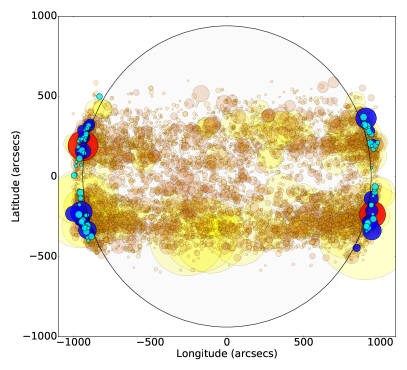
Figure 1: Positions of the partially occulted flares selected in this study (C-Class: light green; M-Class: dark blue; X-Class: red) in context of all C-Class and above flares from the RHESSI flare catalog until the end of 2015 (yellow and orange). The size of the circles is scaled with the observed GOES level and the solar limb is drawn at 940 arcsecs to guide the eye. We omitted outliers with Solar-Y greater or smaller than $\pm 600$ arcsecs, as being unphysical.

For the purpose of this study we extended the list of partially occulted flare candidates to cover solar cycles 23 and 24. Our study is based on two joined data sets. For the time interval from March 2002 until August 2004 we used the same selection of flares as discussed in KL2008 and included them in our analysis. The second data set is based on partially occulted flare candidates in the RHESSI flare catalog, covering flares simultaneously observed by SDO, from January 2011 until December 2015.

2.1 Flare selection

The candidate flares with occulted footpoints were selected from the RHESSI flare list as those flares with significant counts at energies of 25 keV and higher and being close to the solar limb (centroid position $\sim 930-1050$ arcsec with respect to the solar center).

Using SDO/AIA, STEREO and RHESSI, we inspected the emission in the hot corona and X-rays of approximately 400 candidates to visually determine which ones are actually occulted in their footpoints. We aimed to avoid false-positives, i.e. flares which are not truly occulted, as much as possible in our selection, to prevent contamination of footpoint emission in our spectral analysis. As such, this selection can be regarded as a conservative lower limit approximation to all the actually partially occulted flares observed by RHESSI. We nevertheless expect no significant biases in our selection, but the overall sample size has to be kept in mind.

Table 1 gives a list of 61 flares from solar cycle 24 satisfying our selection criteria with date, time, GOES classification (directly measured and estimated with STEREO), and longitudinal/latitudinal centroid position in the higher energy range according to the RHESSI flare list. We also list the main parameters resulting from our spectral, light-curve and imaging analysis, as described in the following sections (the results for the 55 KL2008 flares are listed in Table 2).

Figure 1 gives an overview of the positions of our selection of flares, in the context of all flares observed by RHESSI (C-class and above). The circle size is scaled proportionally to the observed GOES class.

Table 1: Partially occulted flares from solar cycle 24. See Table 2 in the Appendix for the flare list from the previous cycle.

#	Date	Time	GOES Class		Sol-X	Sol-Y	$H$	$T_{th}$	$E_{break}$	$\gamma$	$T_{th}^{\kappa}$	$T^{\kappa}$	$\kappa$	$d_{max}$	Lin.	Lag
		(UT)	Orig.	STER.	(arcs.)	(arcs.)	(Mm)	(MK)	(keV)		(MK)	(MK)		(Mm)	Corr.	(s)
1	2	3	4	5	6	7	8	9	10	11	12	13	14	15	16	17
1	2011 Jan 28	00:57:03	M1.3	M9.3	937.7	285.6	3.7	20.1	15.6	4.73	18.2	12.9	4.33	-1.2	0.81	0
2	2011 Mar 08	18:12:43	M4.4	M7.6	932.0	-287.6	6.3	25.0	18.4	4.68	18.0	12.4	4.30	-1.6	0.93	0
3	2011 Jun 12	17:07:47	B8.6	C2.4	-915.7	275.3	16.6	19.2	13.1	7.74	-	-	-	0.5	-	-
4	2011 Sep 06	06:00:25	C9.6	X1.7	890.7	370.6	24.4	19.6	16.3	7.32	12.9	14.0	7.90	-0.8	-	-
5	2012 Aug 17	08:33:04	C4.7	C9.5	-902.2	318.4	3.7	22.2	18.0	3.75	18.5	8.0	2.87	1.9	0.72	-16
6	2012 Aug 17	13:17:50	M2.4	M3.9	-898.8	316.9	3.7	24.4	21.4	5.03	22.0	5.6	5.42	1.1	0.85	0
7	2012 Sep 30	23:38:36	C9.9	M2.8	934.4	206.0	5.7	25.2	-	-	-	-	-	0.8	-	-
8	2012 Oct 07	20:24:48	C1.2	M6.0	-928.6	287.6	18.2	34.2	12.3	4.13	21.2	26.8	5.70	0.6	-	-
9	2012 Oct 17	07:53:55	C7.4	M2.1	-960.8	112.9	7.4	31.0	11.3	4.11	19.2	19.1	4.30	-0.8	-	-
10	2012 Oct 20	18:12:12	M9.0	M7.1	-949.4	-222.9	7.9	24.8	18.7	7.63	28.1	15.8	7.39	0.9	0.86	8
11	2013 Apr 11	22:50:23	C4.0	M2.6	955.7	169.5	15.1	25.2	17.6	6.36	22.0	9.9	5.10	-2.1	-	-
12	2013 May 12	22:41:06	M1.3	C5.4	-945.4	167.3	12.6	26.6	19.5	6.84	22.7	19.9	7.54	0.1	-	-
13	2013 May 13	01:59:15	X1.7	X1.5	-938.0	192.2	13.3	28.6	19.9	5.79	16.1	21.6	7.31	0.9	0.70	4
14	2013 Jul 29	23:25:48	C6.3	C9.3	963.5	-97.8	-	17.6	13.5	8.38	-	-	-	-	-	-
15	2013 Aug 22	05:11:32	C3.3	C7.6	962.3	-83.8	7.5	20.2	-	-	-	-	-	-	-	-
16	2013 Oct 14	21:46:13	C3.0	C6.9	-970.4	184.1	20.1	22.9	-	-	-	-	-	-	-	-
17	2013 Nov 15	10:00:08	C1.8	M2.2	-926.2	253.7	24.1	23.6	-	-	-	-	-	-	-	-
18	2013 Dec 25	18:56:52	B9.3	C1.0	965.4	-285.4	8.8	23.7	-	-	-	-	-	-	-	-
19	2013 Dec 31	04:45:44	C1.4	C3.7	-967.3	-89.2	24.0	25.9	-	-	-	-	-	-	-	-
20	2014 Jan 16	15:18:13	C2.8	-	-909.0	-382.4	26.1	18.7	12.6	6.70	-	-	-	-2.1	-	-
21	2014 Jan 17	08:28:12	C2.2	-	-903.1	-400.3	9.4	19.7	12.9	6.46	21.9	6.5	4.74	0.9	-	-
22	2014 Jan 27	22:09:24	M4.9	M3.1	-946.8	-260.6	1.9	14.8	14.8	6.13	7.5	8.7	6.02	1.4	0.77	0
23	2014 Mar 14	10:09:44	C5.0	M1.4	942.5	262.7	9.4	27.1	-	-	-	-	-	-	0.39	24
24	2014 Apr 23	08:38:08	C1.6	C6.4	943.0	54.3	14.1	33.1	-	-	-	-	-	-	-	-
25	2014 Apr 25	00:20:36	X1.3	X2.6	949.3	-237.9	11.3	13.8	14.2	3.68	10.1	4.3	2.70	4.4	0.81	-12
26	2014 May 07	06:27:26	C3.6	M2.2	946.3	-175.6	11.0	17.2	13.2	5.92	17.1	7.4	6.03	-0.8	-	-
27	2014 Jun 08	09:52:08	C2.0	-	-920.3	-298.3	37.7	22.2	-	-	-	-	-	-	-	-
28	2014 Sep 03	13:35:36	M2.5	M1.7	-940.6	-269.9	19.1	22.0	17.1	5.88	21.2	15.8	7.06	2.8	-	-
29	2014 Sep 11	15:23:37	M2.1	M4.3	-926.7	245.7	4.4	26.5	19.3	3.22	26.2	6.5	2.28	0.9	0.78	-12
30	2014 Sep 11	21:25:02	M1.4	M1.7	-925.9	246.1	4.0	23.0	18.1	4.67	18.2	11.2	4.19	-0.7	0.77	-4
31	2014 Oct 02	22:53:43	C3.8	-	921.5	-280.3	-	19.4	16.6	4.59	15.1	4.2	4.14	-1.9	0.34	20
32	2014 Oct 22	15:52:49	M1.4	-	-957.1	-203.3	-	20.0	17.5	4.01	19.2	6.7	3.39	4.0	-	-
33	2014 Oct 31	00:35:05	C8.2	-	954.2	-265.8	-	30.1	19.6	6.59	30.7	12.6	5.81	-6.2	-	-
34	2014 Nov 03	11:37:00	M2.2	-	-938.6	288.1	-	19.9	16.6	5.32	17.0	10.6	5.20	2.2	-	-
35	2014 Dec 25	08:46:57	C1.9	-	950.8	-234.7	-	34.5	17.2	4.50	30.1	9.5	3.47	-0.2	0.63	16
36	2015 Mar 03	01:32:05	M8.2	-	906.5	363.0	-	25.6	18.8	6.76	28.9	10.4	3.76	-0.1	0.95	0
37	2015 Mar 21	00:14:52	C1.4	-	909.5	-342.7	-	34.3	-	-	-	-	-	-	0.47	16
38	2015 Mar 30	19:29:56	C1.0	-	916.4	321.6	-	26.2	-	-	-	-	-	-	-	-
39	2015 Apr 13	04:07:49	C4.3	-	-910.9	300.7	-	24.4	18.8	4.47	21.7	6.6	3.63	-2.5	0.84	4
40	2015 Apr 23	02:08:29	C2.2	-	945.2	189.2	-	17.9	13.3	7.53	-	-	-	-	-	-
41	2015 May 04	02:53:30	C3.0	-	-925.4	227.1	-	33.2	19.1	5.78	11.0	14.7	5.29	0.4	0.91	0
42	2015 May 04	17:01:57	C5.1	-	-930.0	242.6	-	30.6	23.2	4.33	24.0	14.1	5.54	-3.9	0.57	0
43	2015 Jun 09	18:52:09	B7.7	-	-896.5	-325.3	-	24.3	-	-	-	-	-	-	-	-
44	2015 Jun 10	21:25:56	C1.5	-	-898.3	-320.0	-	25.0	-	-	-	-	-	-	-	-
45	2015 Jun 11	18:04:46	C1.8	-	-950.7	73.2	-	26.9	13.9	3.43	13.9	6.2	3.76	0.6	-	-
46	2015 Jun 15	00:46:23	C1.0	-	919.8	233.0	-	23.7	-	-	-	-	-	-	-	-
47	2015 Jun 28	17:12:28	C1.9	-	-914.6	250.6	-	19.7	13.4	8.48	-	-	-	-	-	-
48	2015 Jul 14	12:06:25	C1.2	-	-920.3	241.2	-	26.4	-	-	-	-	-	-	-	-
49	2015 Oct 04	02:38:37	M1.0	-	914.7	-323.9	-	21.3	16.4	5.50	16.2	15.0	5.86	-1.2	0.61	0
50	2015 Oct 16	21:56:44	C1.1	-	-968.2	158.5	-	23.3	-	-	-	-	-	-	-	-
51	2015 Oct 17	01:23:24	C3.4	-	-920.5	-311.3	-	27.1	-	-	-	-	-	-	-	-
52	2015 Oct 17	18:35:57	C8.6	-	-916.5	-344.7	-	25.6	-	-	-	-	-	-	-	-
53	2015 Oct 17	23:16:22	C6.6	-	-927.4	-321.3	-	22.7	-	-	-	-	-	-	-	-
54	2015 Oct 30	14:46:09	C3.4	-	982.1	211.8	-	10.7	10.0	3.80	-	-	-	-3.1	-	-
55	2015 Dec 09	10:53:48	C1.2	C4.4	-953.5	-245.5	-	24.7	-	-	-	-	-	-	-	-
56	2015 Dec 12	05:06:57	C4.9	M1.1	-956.2	229.9	10.0	34.6	-	-	-	-	-	-	0.63	16
57	2015 Dec 12	11:42:48	C2.2	C2.7	-966.1	216.8	9.5	32.4	-	-	-	-	-	-	0.58	8
58	2015 Dec 19	13:03:35	C1.7	M8.2	-981.7	90.6	51.7	20.6	12.4	4.35	-	-	-	1.3	-	-
59	2015 Dec 20	05:01:20	C2.4	M1.2	-983.9	65.5	17.3	18.4	-	-	-	-	-	-	-	-
60	2015 Dec 20	12:40:09	C2.0	-	-986.4	12.4	17.1	21.9	-	-	-	-	-	-	-	-
61	2015 Dec 20	22:37:00	C6.1	M1.1	-996.8	6.9	15.0	22.9	12.7	7.36	-	-	-	-4.9	0.48	0

2.2 Time profiles

We analyzed the time evolution of the hard X-ray flux measured by RHESSI and compared it with the temporal derivative of the soft X-ray flux measured by GOES in both the high ($0.5-4$ Å) and low ($1-8$ Å) energy channels for all selected events. Focusing on higher energy RHESSI emission, we calculated the linear correlation between soft and hard X-rays (the so-called Neupert effect, Neupert, 1968).

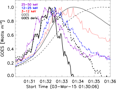
Figure 2: Temporal evolution of the soft X-ray time derivative and the hard X-ray RHESSI count rates in three energy ranges (red, blue and purple). The GOES high energy ($0.5-4$ Å) and low energy ($1-8$ Å) fluxes are plotted as solid and dashed grey lines, while their derivatives are given by the respective black lines. All quantities are normalized to their maximum values in the time interval.

Figure 2 shows an example of the temporal evolution of the soft and hard X-ray flux in different GOES and RHESSI energy channels. It can be seen that the two RHESSI lowest energy channels are delayed with respect to the GOES derivatives. The high energy channel at $25-50$ keV has a quick rise to maximum and correlates well with both GOES derivatives during the rise phase. Later, during the decay phase, the lower energy soft X-rays decay slower, implying a longer cooling timescale. A cross-correlation analysis showed a correlation coefficient of 0.95 for this high-energy RHESSI channel and the $0.5-4$ Å GOES derivative and no substantial lag. The correlation of the low-energy GOES channel with the RHESSI $25-50$ keV band is slightly worse (0.80) but equally good when comparing with the RHESSI $12-25$ keV light curve. This represents a clear example of a strong correlation in our study.

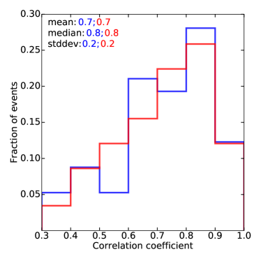
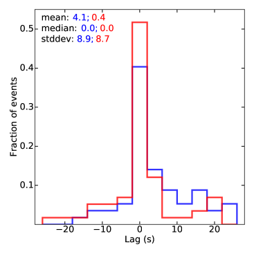
Figure 3: Correlation coefficients (left) and temporal lags (in s, right) for our complete ensemble of partially occulted flares as calculated from the light curve cross-correlation analysis of the GOES soft X-ray time derivative (low channel: red; high channel: blue) and the RHESSI hard X-ray flux. Positive lags imply an earlier rise in soft X-rays compared to hard X-rays.

By discarding all the thermal events (cf. Section 2.5) and those with incomplete GOES or RHESSI light-curve coverage, 57 events remained for the GOES correlation analysis in this study (the discarded values are labeled with a dash in Tables 1 and 2). Figure 3 presents a histogram of the correlation and lag between the best-fitting high energy RHESSI channel and the GOES soft X-ray time derivatives. Many flares show a good correlation and a small number of lags has a tendency towards positive values meaning that the rise in the derivative of the high energy channel soft X-rays occurs earlier than the hard X-ray emission. Most of the flares with strong correlations do not show a significant lag.

2.3 Imaging

RHESSI’s unique imaging capability allows a detailed study of the spatial structure of the hard X-ray emission. We consider 20 seconds around the first peak of the flare in the highest energy range with increased count rate to be our interval of interest (see column 3 of Tables 1 and 2), avoiding attenuator changes when needed. For every flare in our list, we created images in a low energy (typically $\sim$ 6-14 keV) and high energy (typically $>20$ keV) range, using the CLEAN algorithm (Hurford et al., 2002) and a combination of detectors suitable for imaging in that time interval (usually a subset of detectors 3-8). This avoids detectors not properly segmented at a given time. Some flares with no clear high-energy signal (typically lower than 22 keV) did not allow for such analysis. They were discarded from this part of the statistical study. These ‘thermal’ flares, as shown in the tables, have only temperature values as derived from a purely thermal fit. When selecting the range for the high-energy component, we carefully checked that the break energy as inferred from the broken power-law spectral analysis (cf. Section 2.5) is at least 4 keV (or 4 energy bins) lower than the lower boundary of our energy interval.

Apart from confirming that there is no visible footpoint emission for a particular flare during this time, these images allow to estimate the radial separation between the thermal and non-thermal emission. We determined the distance $d_{max}$ between the maxima and distance $d_{com}$ between centers of mass of the low and high energy images. Positive values indicate that the non-thermal source is located farther away from the limb than the thermal component. The resulting values for $d_{max}$ are reported in Tables 1 and 2. The values for $d_{com}$ are generally very similar.

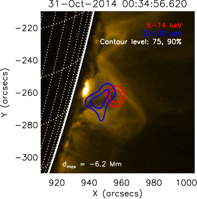
Figure 4: Background AIA 131 Å emission and RHESSI X-ray (CLEAN algorithm) contours at 6-14 keV (red) and 22-30 keV (blue). Left: Coronal emission of the M1.4 class flare that occurred on October 22, 2014 with high energies at larger radial distance than low energies. Right: Emission of the C8.2 class flare from October 31, 2014 having inverted radial positions.

Figure 4 (left) shows an image of the October 22, 2014 M1.4 class flare as an example. We find a positive radial separation of about 4 Mm between the two energy maxima, meaning that the non-thermal source is at higher altitude. The coronal emission at 131 Å shows multiple bright loops. The higher energy, mostly non-thermal X-ray emission is near the top of the coronal loops. Other AIA wavelength don’t show the loops as clearly, indicating that they are hot with temparatures of about 10 MK. This radial ordering of low and high energy emission is expected from standard flare scenarios, since the non-thermal particles are presumably produce close to the reconnection region above the thermal loop top (e.g. Krucker et al., 2008).

However, we found for a few flares in our sample that the high-energy emission is centered closer to the limb than the lower energies. The right panel of Figure 4 gives an example. The C8.2 class flare from October 31, 2014 has an extended high-energy emission region below a relatively compact thermal source, which is about 6 Mm higher in the corona. In this particular case, the high-energy emission coincides with a dark structure in the 131 Å AIA channel (also clearly visible e.g. in 335 Å). A possible explanation for the emission there is thus that it acts as dense target above the chromosphere for the non-thermal particles. Alternatively, the bright EUV emission close to the limb could indicate that we only see the above-the-looptop part of the X-ray emission (e.g. Liu et al., 2013), which would show such an inverted ordering of low and high energies.

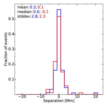
Figure 5: Frequency distribution of the separation between the low and high energy X-ray sources as quantified by their emission maximum ($d_{max}$, blue) and center of mass ($d_{com}$, red), resulting from the imaging analysis. Positive values indicate that the non-thermal source is located farther away from the limb than the thermal component.

Figure 5 gives a histogram of separation estimates $d_{max}$ and $d_{com}$ between low and high energies. The two estimates do not differ significantly from each other. We find no clear tendency towards positive or negative separations between the low and high energy sources. The mean of $d_{max}$ is 0.3 Mm, indicating a possible trend that the higher energy emission might radially be farther out in the corona, but this value is still consistent with no separation.

2.4 STEREO Analysis: Height and GOES-class

The twin STEREO-A and B spacecraft allowed us to confirm for many of the flares in our cycle 24 sample that the associated active regions and footpoints were indeed located behind the limb. We were also able to estimate the heights of the X-ray sources and the true (un-occulted) soft X-ray magnitudes of the flares. However, depending on the STEREO positions, and the quality and cadence of their data, these estimates were not always obtainable, particularly from October 2014 to November 2015, when both STEREO spacecraft were on the opposite side of the Sun near the Sun-Earth line and had limited or no telemetry.

By combining the line of sights of the emissions seen by RHESSI and STEREO into a 3D structure, we estimated the height of the coronal emission. The geometry is illustrated in Figure 6. The line-of-sight from Earth towards the source (‘L1’) and the radial (‘L2’) from the center of the Sun through the brightest point of the active region (AR), as selected from STEREO observations, do not necessarily intersect in 3D space (the X-ray source may not be directly above the AR). To estimate a source altitude above the photosphere, a vector was drawn from the AR to the midpoint of the shortest possible line segment connecting both L1 and L2. The projection of that vector on the local vertical gives the estimated heights $H$ of the coronal emission. These values are given in column 8 of Table 1, with a mean of 14 Mm and a median height of 11.3 Mm, consistent with a typical loop size.

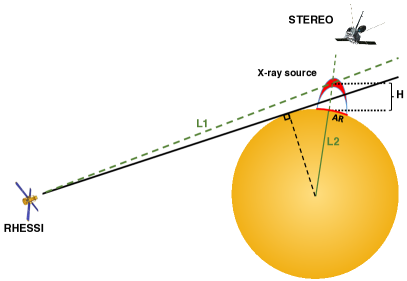
Figure 6: Two-dimensional sketch to illustrate the geometry of view angles and the calculation of the flare height $H$ with combined RHESSI and STEREO information.

The temporal evolution of the STEREO 195 Å emission allowed us to extrapolate to other wavelengths and estimate the soft X-ray magnitude of the flare, as if it would be an on-disk event. This was done using the empirical relation between the peak STEREO 195 Å flux and the GOES 1 – 8 Å soft X-ray flux (Nitta et al., 2013, Eq. (1) and their Figure 7):

$$F_{\rm GOES}=1.39\times 10^{-11}F_{\rm EUVI(195)},$$ (1)

where $F_{\rm GOES}$ is the GOES 1 – 8 Å channel flux in units of [W m^-2] and $F_{\rm EUVI(195)}$ is the pre-event background subtracted STEREO 195 Å flux in [DN s^-1].

The resulting GOES class estimates are reported in column 5 of Table 1, along with the actual GOES class observed from Earth in column 4. In general, these estimates show that the latter often significantly underestimate the true magnitude of the flare. However, we note that there are a few outliers from this general trend. That is, the estimated GOES class can be lower in some instances than the observed class from Earth. There are at least two possible causes of this discrepancy. First, equation 1 is an empirical relation that has certain ranges of uncertainties, which are within a factor of three for flares $>$M4 class and an order of magnitude for less intense flares. Second, in case of low-cadence ($\geq$10 minutes) observations, STEREO can miss the true EUV peak and thus underestimate the flare class.

2.5 Spectral analysis

Two kinds of spectral analysis were performed for every flare in our list, followed by detailed checks of the goodness-of-the fit and re-analysis when necessary. All fits were done with the standard Object Spectral Executive (OSPEX) software package (e.g. Schwartz et al., 2002). The fitting time interval is the same 20s around the first non-thermal peak as described for imaging. By using an initially automated procedure, we have a better comparability of fitting results between different flares.

(1) The first fitting model is a fit of the observed photon spectrum by a thermal plus broken power-law model (hereafter, th-bpow), similar to that used in KL2008, which has five free parameters: the emission measure, $EM_{th}$, and temperature, $T_{th}$, of the thermal component, the normalization, $A_{\gamma}$, the break energy $E_{break}$, and the spectral index, $\gamma$, above the break of the power-law component, $I_{\gamma}(\epsilon)=A_{\gamma}\epsilon^{-\gamma}$. The index below $E_{break}$ is fixed to 1.5 (Holman et al., 2003) and the relative abundances in the thermal component are kept at 1.

(2) The second method fits the observed photon spectrum by bremsstrahlung emission arising from a kappa spectral model for the flux of (non-relativistic) accelerated electrons (th-kappa, Kašparová & Karlický, 2009):

$$F_{\kappa}(E)=A_{\kappa}\frac{{E}}{\sqrt{(k_{B}T_{\kappa})^{3}}}\left(1+\frac{E}{(\kappa-1.5)k_{B}T_{\kappa}}\right)^{-(\kappa+1)}\,.$$ (2)

This model, with three parameters, is a generalization of a non-relativistic Maxwellian distribution with an enhanced non-thermal tail approaching a power law with index $\kappa$ at high energies. However, its thermal component is often not strong enough, especially for low values of the index $\kappa$, to reproduce the prominent thermal component of solar flares at low energies. As a result we had to add an additional thermal component with two additional free parameters, emission measure and temperature, $EM^{\kappa},T_{th}^{\kappa}$, again giving five free fitting parameters (see Oka et al., 2013, 2015, for detailed case studies including an additional thermal component for coronal sources).

An explanation for the necessity of an additional thermal component could be that the emission of the chromospherically evaporated plasma is superimposed onto the in-situ heated component of the kappa distribution in the corona. Imaging spectroscopy can separate different thermal (and non-thermal) parts of the emission (Oka et al., 2015), but since most thermal and non-thermal sources are co-spatial (cf. Section 2.3), in practice this is usually not possible. Battaglia et al. (2015) recently improved the estimation of thermal components by combining emission measures from RHESSI and AIA. This approach may enable further insights into the thermal part of the electron population of coronal sources in future studies.

A key feature of our study is that we fit all available detector spectra separately and combine the resulting parameters of the fit into average quantities. This approach, as detailed in Liu et al. (2008) and Milligan & Dennis (2009), takes advantage of the fact that each detector provides an independent measurement of the X-ray spectrum and avoids smearing in energy of slightly different detector responses. We individually discarded certain detectors for every flare that did not perform properly or showed otherwise strong deviations from the average results.

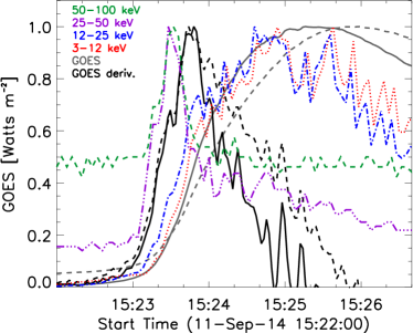
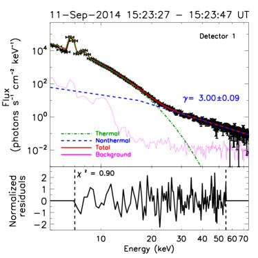
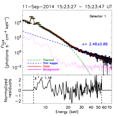
Figure 7: Top left: Coronal emission of the September 11, 2014 M2.1 flare as observed by AIA at 94 Å. The contours correspond to the X-ray emission at low (7-14 keV, red) and high (24-60 keV, blue) energies, using the CLEAN algorithm of Hurford et al. (2002) integrated over 20s around the peak in detectors 3-8. Top right: Light curves of RHESSI count rates at four energy ranges (red, blue, purple and green), GOES high energy flux (0.4 to 5 Å, grey, dash-dotted) and its time derivative (black, solid). The counts in the two high energy channels are multiplied by 20 and 15, respectively, to make them comparable in magnitude. Bottom: Photon spectra as observed by RHESSI detector 1 (15:23:27-15:23:47 UT). The spectrum has been fitted to a thermal component plus a broken power law (left) and a thermal component plus a thin-target kappa distribution function (right).

Figure 7 shows example fit results for both fitting approaches applied to the M2.1 class flare occurred on September 11, 2014, together with the corresponding light curve and imaging analysis. There is no significant spatial separation between thermal and non-thermal coronal emission in this flare and the light curve shows a quick onset of high-energy X-rays with a slightly delayed response in the GOES derivative. The first smaller peak in the GOES derivative is temporally related to the onset of the highest energy (25-100 keV) X-rays detected by RHESSI, while the second, larger peak is associated with a peak at lower energies. The 6-12 keV RHESSI emission aligns well with the temporal evolution of the soft X-rays detected by GOES. Both spectral fits with a broken power law and thin-target kappa function result in a low $\chi^{2}$ value and a good fit over all energies as indicated by the residuals. The high energy broken power-law spectral index $\gamma$ agrees with the expected electron $\kappa$ index within the estimated standard deviation for a thin-target model (see also the discussion below).

The results of our spectral analysis are compiled in Tables 1 and 2, with vertical solid lines separating the two groups of fitting parameters. We note that for some flares, one or both approaches did not converge satisfactorily to a final set of parameters, in which case we left the table empty for these values (‘-’), and discarded them from the statistical analysis.

“Thermal” flares, without clearly distinguishable power-law component at higher energies were fitted only to a pure thermal component. The resulting temperature is reported as $T_{th}$ in both tables instead of the thermal component of the broken power-law fit.

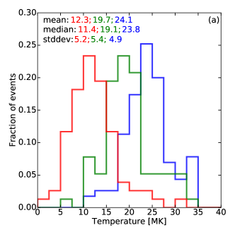
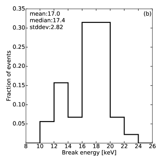
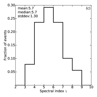
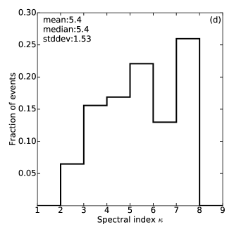
Figure 8: Frequency distributions of fitting parameter results: (a) The three different temperatures, namely the thermal component temperature in the broken power-law fit, $T_{th}$ (blue), the thermal component temperature in the kappa fit, $T_{th}^{kappa}$ (green), and the kappa-temperature $T_{\kappa}$; (b) Break energy of the broken power law $E_{break}$; (c) spectral index $\gamma$ above the break; (d) $\kappa$ values for the th-kappa model.

Figure 8 gives an overview of the statistical properties of the fitting results for our flare sample, combining both solar cycles. The average temperatures are generally ordered from low to high in $T_{\kappa}$, $T_{th}^{\kappa}$, and $T_{th}$. This is most likely due to the fact that the kappa distribution itself has already a thermal contribution. The results for break energies and power-law spectra indexes are in general agreement with the previous results from KL2008, with a tendency to lower break energies in our study. The spectral index $\kappa$ has a broader distribution. The mean values are $\left\langle\gamma\right\rangle=5.7$, similar to the previously reported value in KL2008 of 5.4, and $\left\langle\kappa\right\rangle=5.4$. These are softer than what is found for the high energy index of disk flares, which contain the footpoint emission with harder spectrum (e.g. McTiernan & Petrosian, 1991; Saint-Hilaire et al., 2008; Warmuth & Mann, 2016a, b).

3 Discussion

We now discuss aspects of our flare sample that offer insights into the coronal X-ray source structure and associated energetic electron properties.

As previously mentioned in Section 2.4, we verified that the emission visible from the RHESSI field-of-view had no footpoint contamination according to STEREO, but this approach is also influenced by the location of maximum EUV emission selected in the active region. On the other hand, there are only 36 flares with viable height information from STEREO, leaving the decision on possible chromospheric contamination to the available RHESSI and AIA images, for which we verified that there was no on-disk signatures of footpoints. Thus in what follows we will assume that we are dealing with loop-top emissions in all the flares in the two samples.

It should be also noted that there are differences between the results reported in this study and in KL2008 for the same set of 55 flares (see Table 2). This is due to the combination of several aspects: Our spectral fit approach is partially automated and the initial fitting values and constraints of the variables used for the spectral fits have not been changed unless it appeared necessary. Moreover, the background subtraction and the exact choice of the 20 second fitting interval, aiming for the first peak of the fast time variation component, can influence the results further.

3.1 Thermal vs. non-thermal energy flux

As evident from Tables 1 and 2, a majority of flares have a thermal and a non-thermal component. In general, weaker GOES class flares show a tendency to have only a thermal component and in our two samples, about 20% of flares show no clear non-thermal part. However, most of those are in the new selection from solar cycle 24. Less than 8% of cycle 23 but nearly 40% of cycle 24 are in this category. Part of this difference could be related to the reduced efficiency of the RHESSI detectors, in particular during the later part of 2015 before the anneal procedure in early 2016. On the other hand, our analysis of the time dependence of the spectral fitting parameters shows no significant differences between cycle 23 and 24.

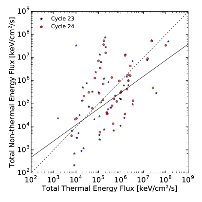
Figure 9: Relation between the total thermal and non-thermal energy flux for the total of 90 flares (discarding all thermal events, cycle 23: blue stars, cycle 24: red circles). The solid line is a linear best fit to a power law with exponent 0.7 and the dashed line indicates equal thermal and non-thermal flux.

A relatively direct way to estimate the importance of the non-thermal emission is to calculate the total energy flux of the thermal (bremsstrahlung) and non-thermal (broken power-law) components of the fits to the observed X-ray spectra.

The total thermal energy flux depends only on the emission measure $EM$ and temperature $T$ of the electrons as:

$$F_{\rm tot,th} = 3\cdot 10^{4}\,\sqrt{\frac{T}{10^{6}\rm{MK}}}\left(\frac{EM}{10^{45}\rm{cm^{-3}}}\right)\,\rm{keV/cm^{2}/s}\,,$$ (3)

while the total energy flux of a broken power law model (in the same units and with low and high energy indexes 1.5 and $\gamma$) is

$$F_{\rm tot,nth} = 450\frac{\gamma-1.5}{\gamma-2}F_{\rm nth}(E_{\rm break})\left(\frac{E_{\rm break}}{15{\rm keV}}\right)^{2}\,,$$ (4)

where $F_{\rm nth}(E_{\rm break})$ is the photon number flux (#/cm²/s/keV) at the break energy.

Figure 9 shows the resulting relation between these energy fluxes for the two flare samples. A correlation (linear correlation coefficient 0.53) can be detected and there is a rough equipartition between energy fluxes. Most electron flare acceleration models starting with a thermal plasma lead to a quasi-thermal plus a power law component (see, e.g. Petrosian & Liu, 2004), with the first producing the thermal and the latter the non-thermal X-rays. Since the bremsstrahlung yield is primarily proportional to the average electron energy ($\propto kT$ and $\propto E_{break}$ for the two components, respectively), and because $kT\sim E_{break}$, we expect a similar relation between the two accelerated components as that between the two photon components.

3.2 Time scales and thin target emission

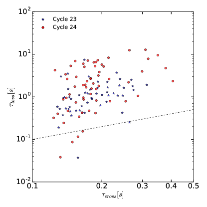
Figure 10: Crossing time ($\tau_{cross}$) and energy loss time ($\tau_{loss}$) as calculated from the areas and densities found for each flare (cycle 23: blue stars, cycle 24: red circles) for 15 keV electrons. Most flares are above the dashed line of equal time scale.

A thin-target model is the correct description for coronal source emission if the time spent by the electrons in the source region is shorter than the energy loss time (mainly due to elastic Coulomb collisions at the non-relativistic energies under consideration here)

$$\tau_{L}=\frac{E}{\dot{E}_{L}}=\frac{\sqrt{2}E^{3/2}}{4\pi r_{0}^{2}n_{e}c\ln{\Lambda}}\,,$$ (5)

where the electron energy $E$ is measured in units of $mc^{2}$, $r_{0}=2.8\cdot 10^{13}$ cm is the classical electron radius and $\ln\Lambda\sim 20$ is the Coulomb logarithm. In absence of field convergence or scattering the time spent in the source or the escape time from it is equal to the time for crossing the source $T_{\rm esc}\sim\tau_{\rm cross}=L/v$, for a source size $L$ and electron velocity $v$. We calculated the ambient electron density $n_{e}$ for each flare from the emission measure of the thermal component in the broken power-law fit ($n_{e}\sim\sqrt{EM/V}$) assuming a filling factor of unity and a spherical source of $V\sim A^{2/3}$, where $A\sim L^{2}$ is the projected area of the $50\%$ image contour.

Figure 10 compares the resulting two time scales for our sample of flares at energy $E=15$ keV, close to the average $E_{break}$. As evident, the thin-target assumption is justified down to break energies for nearly all flares. Note that the distribution in the figure would shift up (down) for higher (lower) electron energies due to the energy dependences in $\tau_{\rm cross}$ and $\tau_{L}$. On average, the two times become comparable at energies below 5 keV where the thin-target assumption would breakdown. In general, there can be some trapping of the electrons so that the time they spend at the loop top before escaping to the footpoints, $\tau_{\rm esc}>\tau_{\rm cross}$. This can come about if the field lines converge toward lower heights or there is a scattering agent. Coulomb collisions cannot be this agent because the Coulomb scattering time is comparable to the loss time and therefore its effect will be negligible. Turbulence can provide the scattering. We can only have a low level of turbulence, so that $\tau_{\rm esc}<\tau_{L}$. This appears, for example, to be the case for two non-occulted flares studied by Chen & Petrosian (2013). Using an inversion technique they obtain all the above time scales plus the acceleration and scattering time by turbulence and show that above this condition is satisfied above $\sim 10$ keV and the collision loss time is even longer than acceleration and energy diffusion time above 30 keV.

3.3 The thin-target kappa model

Assuming a thin-target situation we fit the spectra to that expected from electrons with a kappa distribution. Since this distribution contains a quasi-thermal component, we tested several fitting methods. First we fit the spectra to a pure kappa function. We find reasonable fits for most of the flares. But, in general, the $\chi^{2}$ (per free parameters) resulting from this model are higher than those obtained by adding a separate thermal component. Also, as can be expected, the resulting $\kappa$ values are systematically larger for a pure kappa model. Moreover, whenever there is a clear kink separating the thermal and non-thermal energies, the kappa distribution, with a weaker thermal part, especially for low $\kappa$, is not able to properly fit all energy ranges, leading to large residuals at high energies. These cases might indicate that a single thin-target kappa model is not a viable model for many solar flares or that there are multiple distinct plasma populations that are getting combined in the integrated RHESSI spectroscopy. This issue was as already mentioned in KL2008 and followed up in the context of kappa distributions in Oka et al. (2013). In general, we found that for some flares the broken power-law fit adjusts better to the spectra than the kappa distribution.

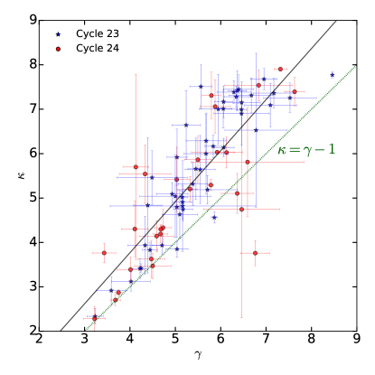
Figure 11: Correlation between the broken power-law photon spectral index $\gamma$ and the electron $\kappa$ index values of the thermal plus thin-target kappa fit for the data of both solar cycles (cycle 23: blue stars, cycle 24: red circles). The black dashed line shows the result of a linear fit to the complete dataset ($\kappa=1.15\,\gamma-0.83$). The green dotted line indicates the theoretical thin target relation.

In Figure 11 we show a plot of $\kappa$ versus the photon index $\gamma$. As evident from Equation (2) (see also Oka et al., 2013), the relation between the electron flux spectral index $\delta$ and the electron kappa distribution index $\kappa$ is just $\delta=\kappa$. As is well known for the thin-target case, we expect the relation $\delta=\gamma-1$, resulting in $\kappa=\gamma-1$. This is shown by the green dotted line in Figure 11. The linear-least-square fit to the whole dataset gives $\kappa=1.15\,\gamma-0.83$ (black-dashed line) which is closer to the expected thin-target relation, particularly for events with clear non-thermal emission signal, i.e. small values of $\gamma$. The discrepancies with the thin-target relation are larger for steep ($\gamma\gtrsim 5$) spectra, which can be attributed to the larger uncertainties when the thermal and non-thermal distribution are difficult to separate. We emphasize that the deviation towards larger than expected values of kappa, based on the thin-target model and relation, mainly indicates the deviations between the two fitting approaches, and cannot support independently a possible thick-target regime (cf. the discussion of time scales in the previous section).

3.4 Temporal correlations and the Neupert effect

A large fraction of flares in our sample shows a good correlation between the derivative of GOES soft X-rays and the RHESSI hard X-ray emission. A good correlation generally implies an absence of substantial lag. However, when there is a lag between the two light curves it tends towards positive values, i.e. an earlier rise in GOES derivative.

The Neupert (1968) effect is a temporal correlation between the soft X-ray flux and the the integral of the microwave flux. The underlying physics of this effect is based on an energy argument (e.g., Li et al., 1993; Veronig et al., 2002, 2005; Ning & Cao, 2010) that the latter depends on the instantaneous flux of non-thermal electrons that deposit their energy (by collisional heating) to the dense chromosphere and drive evaporation of hot plasma that emits soft X-rays. The time integration of the instantaneous energy deposition rate equals the total energy deposited to the thermal plasma, which is reflected in its enhanced temperature and emission measure and thus the soft X-ray irradiance. Therefore, the time derivative of the soft X-ray flux is expected to be correlated with the instantaneous hard X-ray flux. Since the energy deposited by accelerated electrons is related to the observed hard X-ray emission via the escape time $T_{esc}$, we have as a restriction that we can only observe the simple Neupert effect as long as $T_{esc}$ is independent of time.

As pointed out by Liu et al. (2006), neither the non-thermal bremsstrahlung X-ray emission is a linear function of the collisional energy deposition rate, nor the thermal X-ray emission depends linearly on the total energy content of the thermal plasma. Therefore, a perfect linear correlation for the Neupert effect is not expected. In addition, the above energy argument is based on the assumption that non-thermal electrons are the sole agent of energy transport from the coronal loop-top to the footpoints. This is not necessarily the case either, because other mechanisms, including thermal conduction, can play some role and cause further deviations of the temporal correlation (e.g.  Saint-Hilaire & Benz, 2005, found the ratio between non-thermal to thermal energies to increases with flare duration). In particular, the slightly preferential positive lag of the hard X-ray flux from the GOES derivative suggests that in those flares substantial soft X-ray emitting thermal plasma is present prior to the acceleration of non-thermal electrons, which implies non-collisional heating mechanisms such as thermal conduction (Zarro & Lemen, 1988; Battaglia et al., 2009) or turbulence (Petrosian & Liu, 2004). On the other hand, the existence of negative lags for a small fraction of the flares is consistent with the finding of Liu et al. (2006), who ascribed this to hydrodynamic timescales for the deposited non-thermal energy to drive chromospheric evaporation of thermal plasma.

Despite the expectation that the partial occultation of soft X-ray emitting plasma and footpoint hard X-rays can potentially cause further deviations from the perfect Neupert effect compared with on-disk flares, we do find strong correlations. This provides additional support for the scenario that the primary particle acceleration site is at or near the coronal X-ray source, rather than at the chromospheric footprints (e.g., Fletcher & Hudson, 2008).

3.5 Source Morphologies

As mentioned in Section 2.3, there is no clear trend towards positive or negative separations between low and high energy source positions. The average separation is $d_{max}$=0.3 Mm, which is not statistically significant. This result is in agreement with the previous findings by KL2008. The trend is, however, inconsistent with several individual case studies of coronal X-ray sources, which found, in general, that the higher energy emission is located at greater heights (e.g., Sui & Holman, 2003; Sui et al., 2004; Liu et al., 2004, 2008, 2009). We found in certain flares of our sample that there are multiple sources above the loop-top (see e.g Figure 4). More detailed studies of such events can be found in Liu et al. (2013), Krucker & Battaglia (2014), Oka et al. (2015), and Effenberger et al. (2016). A few flares showed also high-energy emission coming from regions lower in the corona than the location of the low-energy centroid. A possible explanation for this feature is a situation in which the flare loop is very occulted, so that only the above-the-looptop sources are visible. In this situation, the high energy emission is closer to the reconnection region and thus to the limb (Liu et al., 2013; Oka et al., 2015).

4 Summary

We have analyzed X-ray light curves, images and spectra of 116 partially occulted flares during solar cycle 23 and 24. The additional availability of SDO and STEREO observations during cycle 24 allowed for supplementary information to characterize the limb flares. EUV observations from STEREO allowed us to estimate the actual GOES classification and the high-cadence AIA images helped to confirm the actual occultation of the flare with greater confidence and provided valuable context for the interpretation of the individual flare evolution. From STEREO we further obtained the position of the active region and determined the height of the coronal source. Our results can be summarized as follows:

1. We found no significant difference in the statistics of the derived flare properties between the two cycles.

2. We use a thermal plus a power-law (with index $\gamma$) model to describe the RHESSI X-ray spectra. Most flares are dominated by the thermal component and about 20% show no discernible non-thermal part. From the spectral fitting parameters (emission measure, temperature, break energy and power-law spectral indexes) we compared the emitted energy fluxes (during 20 second around the impulsive phase) in thermal and non-thermal photons. We found some correlation and comparable energies. Using the density of the thermal component (derived from the emission measure and size of the source) we found that the energy loss time is much longer than the free source crossing time indicating that we are dealing with a thin-target model.

3. We also fitted the photon spectra by a thin-target bremsstrahlung emission model from electrons with a kappa distribution, which consists of a Maxwellian plus a non-thermal component (with high energy index $\kappa$). Although reasonable fits are obtained in this procedure, we found that the electrons in the Maxwellian part often cannot describe the prominent thermal component of the photon spectra adequately, and that better fits can be obtained by the addition of a more prominent thermal source. We found that the spectra of occulted flares tend to be softer than general disk flares with the relation between the photon and electron indexes, $\kappa=1.18\gamma-0.84$ to be in rough agreement with that expected in a thin-target model at lower values for the spectral index. It deviates significantly from this relation for high values of the indexes where the spectra are dominated by the thermal component and errors are large.

4. We found no trend for large spatial separations between low and high energy hard X-ray components in the spectral images of our sample. There are, however, notable exceptions with larger separations and a richer coronal source structure. The estimations of source height and GOES classification with STEREO observations reveal a large variety of coronal source positions with heights up to 52 Mm and differences in GOES class showing for example a strong C class flare to be actually a X class flare.

5. We found a significant correlation between the time derivative of the soft X-ray and the observed hard X-rays light curves for a large fraction of our sample, with a mean lag time of near zero, consistent with earlier studies for on-disk flares (Veronig et al., 2002). This confirms the presence of the simple Neupert effect for purely coronal sources and supports the scenario that the main source of non-thermal particles is produced near the looptop. The lags found in some flares indicate that additional processes like thermal conduction can play important roles.

As mentioned at the outset, partially occulted flares give us direct information on the physical conditions at the acceleration site near the loop-top sources and the spectrum of the accelerated electrons. These can be used to put meaningful constrains on the characteristics of the acceleration mechanisms.

The STIX X-ray instrument on the upcoming Solar Orbiter mission will provide further capabilities to investigate coronal sources of flares from multiple perspectives, allowing us to observe and model the entire flare with greater detail. Hard X-ray focusing optics like FOXSI (Krucker et al., 2013, 2014) can provide simultaneous imaging of the chromospheric footpoints and coronal sources from a single view point due to much improved dynamic range compared to RHESSI and will thus enable additional insights into electron acceleration and transport processes in the corona, even for on-disk flares.

Table 2: Analysis results for partially occulted flares from KL2008

#	Date	Time	GOES	Sol-X	Sol-Y	$T_{th}$	$E_{break}$	$\gamma$	$T_{th}^{\kappa}$	$T^{\kappa}$	$\kappa$	$d_{max}$	Lin.	Lag
		(UT)	Class	(arcs.)	(arcs.)	(MK)	(keV)		(MK)	(MK)		(Mm)		(s)
1	2	3	4	5	6	7	8	9	10	11	12	13	14	15
1	2002 Mar 07	17:50:44	C2.5	-961.5	-176.4	21.4	11.6	5.86	32.0	10.1	4.56	-0.4	0.77	12
2	2002 Mar 28	17:56:07	C7.6	965.7	-64.2	21.6	17.6	5.55	15.6	12.9	5.64	-0.6	0.66	-4
3	2002 Apr 04	10:43:52	M1.4	-896.8	-347.5	25.4	18.8	5.16	16.9	11.0	4.91	0.5	0.86	0
4	2002 Apr 04	15:29:14	M6.1	-909.3	-333.8	27.0	19.6	5.17	26.5	9.8	4.75	0.7	0.87	4
5	2002 Apr 18	06:52:04	C9.4	913.7	314.1	19.9	17.0	5.38	18.3	9.9	5.32	3.7	-	-
6	2002 Apr 22	12:05:56	C2.8	900.2	-319.3	20.9	15.8	4.02	20.6	7.6	3.12	3.5	-	-
7	2002 Apr 29	13:00:55	C2.2	-904.5	-323.6	10.1	13.3	8.06	-	-	-	0.0	-	-
8	2002 Apr 30	00:32:48	C7.8	-882.8	-373.7	20.9	18.6	5.68	18.6	7.1	6.00	0.5	-	-
9	2002 Apr 30	08:20:44	M1.3	-891.5	-357.5	23.0	17.8	5.15	20.2	10.3	5.02	1.4	0.87	0
10	2002 May 17	02:01:28	C5.1	-929.5	227.5	26.0	17.5	4.49	19.3	11.3	5.46	0.0	-	-
11	2002 May 17	07:32:40	M1.5	-931.2	230.2	26.6	19.9	6.06	17.3	17.5	7.17	1.1	0.47	-8
12	2002 Jul 05	08:03:06	C7.8	917.3	-291.2	20.8	19.1	7.53	19.1	11.0	7.26	0.5	-	-
13	2002 Jul 06	03:32:15	M1.8	911.6	-281.4	24.9	18.9	5.56	21.7	31.8	7.51	2.1	-	-
14	2002 Jul 08	09:15:39	M1.6	-891.8	330.5	22.8	18.1	5.45	17.6	12.6	5.66	1.6	0.52	4
15	2002 Jul 09	04:03:28	C8.6	896.3	322.4	20.9	-	-	-	-	-	-	0.60	24
16	2002 Aug 04	09:38:51	M6.6	945.1	-338.0	21.0	18.8	8.46	23.9	12.0	7.77	-0.9	-	-
17	2002 Aug 04	14:14:48	C6.9	909.5	-310.7	23.2	18.3	6.95	15.2	14.5	7.68	1.3	0.66	0
18	2002 Aug 28	18:54:44	M4.6	-937.9	158.3	32.5	19.0	4.44	32.9	9.8	3.83	0.1	0.60	12
19	2002 Aug 28	21:43:23	M1.1	845.4	-445.7	26.7	19.4	5.04	26.1	8.8	4.80	0.7	0.49	0
20	2002 Aug 29	02:50:28	M1.6	-946.9	141.5	26.2	20.2	5.83	20.6	9.9	6.17	1.0	0.74	8
21	2002 Aug 29	05:43:56	C9.2	840.3	449.9	33.7	21.9	5.24	28.5	23.1	6.64	0.0	0.88	4
22	2002 Sep 06	16:27:00	C9.2	-954.6	-101.7	23.5	16.7	4.22	22.4	6.4	3.41	-1.7	0.88	0
23	2002 Oct 16	15:57:20	C6.5	-830.4	499.6	23.8	17.9	6.78	17.9	21.7	6.53	-1.5	-	-
24	2002 Nov 15	01:08:36	M2.4	-931.9	-290.0	24.5	18.4	5.95	14.9	14.7	7.00	2.1	0.93	0
25	2002 Nov 23	01:21:40	C2.1	-946.6	234.5	22.0	16.6	5.00	21.0	13.2	5.04	0.9	-	-
26	2003 Jan 21	01:25:51	C2.0	-935.8	-299.2	31.2	-	-	-	-	-	-	-	-
27	2003 Feb 01	08:57:28	M1.2	-966.4	-251.1	25.3	18.1	6.37	16.2	16.4	7.42	7.7	0.86	4
28	2003 Feb 01	19:41:33	C9.9	-965.3	-237.4	33.9	16.6	7.39	-	-	-	0.5	-	-
29	2003 Feb 14	09:16:15	M1.2	955.0	207.1	24.5	19.1	5.68	21.6	10.5	6.29	0.0	0.76	4
30	2003 Mar 27	14:52:04	C2.3	925.5	299.5	27.4	11.2	4.39	23.2	17.2	4.84	-0.7	0.64	16
31	2003 Apr 24	04:53:44	C7.1	925.3	279.9	20.9	17.2	6.06	14.3	16.0	7.01	-0.7	0.83	0
32	2003 Apr 24	06:35:08	C1.0	907.6	267.9	29.6	17.2	3.59	19.9	12.5	2.92	-0.7	0.88	0
33	2003 May 07	20:47:48	C5.9	-916.8	263.8	22.8	19.0	7.09	18.9	12.9	7.09	2.5	0.94	0
34	2003 Jun 01	12:48:32	M1.0	-936.6	172.3	28.7	20.4	4.93	19.3	9.4	5.09	-1.0	0.87	-8
35	2003 Jun 02	08:15:12	M3.9	940.1	-137.5	22.6	17.2	5.04	18.1	12.7	5.92	0.0	-	-
36	2003 Jun 06	16:17:10	C2.5	-920.2	-243.6	17.5	13.4	8.35	-	-	-	-0.3	0.76	12
37	2003 Aug 21	15:19:02	C4.9	940.4	-178.6	22.9	16.9	4.33	21.6	9.0	3.94	0.1	-	-
38	2003 Sep 15	16:38:51	C1.5	953.6	-122.4	22.4	13.1	6.54	-	-	-	-0.9	0.70	0
39	2003 Sep 29	16:09:07	C5.1	-953.8	-136.6	20.9	17.2	6.68	18.9	14.5	7.31	-1.7	0.66	4
40	2003 Oct 21	23:07:04	M2.4	-945.8	-277.8	26.0	20.0	6.46	12.1	11.0	7.15	2.5	-	-
41	2003 Oct 22	18:43:08	C6.0	-937.2	-285.1	24.5	17.2	7.17	26.1	11.4	7.36	0.3	-	-
42	2003 Oct 22	21:56:24	M2.1	-943.0	-284.7	23.6	17.4	6.40	15.3	17.3	7.45	-0.5	0.83	0
43	2003 Oct 23	01:06:24	C4.0	-938.8	-291.9	-	-	-	-	-	-	-	-	-
44	2003 Nov 04	14:47:28	C7.5	967.9	161.7	24.5	17.6	6.29	11.3	18.5	7.39	-1.7	-	-
45	2003 Nov 04	15:30:08	C5.6	956.5	187.4	18.9	17.1	4.71	15.7	8.3	3.93	0.2	0.47	24
46	2003 Nov 05	01:58:53	C7.2	965.8	170.0	28.7	16.3	5.10	28.2	9.6	4.63	-1.5	-	-
47	2003 Nov 18	09:43:58	M4.5	-1002.4	-232.2	16.5	15.2	6.46	15.5	11.8	6.99	19.7	-	-
48	2003 Nov 18	22:17:41	C6.1	-939.6	-271.2	29.4	14.9	3.23	20.4	15.9	2.34	-0.3	0.71	0
49	2003 Nov 19	10:07:18	C2.7	-931.5	-272.9	13.2	11.1	5.04	11.5	0.3	3.85	-0.6	0.78	8
50	2004 Mar 05	08:54:21	C6.6	-948.0	-282.7	29.1	20.5	5.16	20.7	11.5	4.82	-1.4	0.35	8
51	2004 Mar 24	23:25:22	M1.5	-941.1	245.6	24.4	19.3	6.34	15.6	12.7	7.28	0.0	0.62	20
52	2004 Jul 15	22:27:05	C7.9	-944.0	162.6	29.8	19.5	6.46	30.7	22.9	6.90	-1.3	0.91	0
53	2004 Jul 17	03:46:25	C4.2	-930.5	146.2	22.0	17.3	4.24	15.6	10.5	3.42	-0.9	0.81	16
54	2004 Aug 18	08:41:05	C6.1	936.2	-212.2	27.2	18.8	5.71	11.7	12.5	5.19	-0.6	0.61	-4
55	2004 Aug 19	06:54:04	M3.0	943.0	-213.2	28.4	22.6	6.07	17.6	10.2	6.14	0.7	0.90	0

References

- Bai et al. (2012) Bai, W.-d., Li, Y.-p., & Gan, W.-q. 2012, Chinese Astron. Astrophys., 36, 246
- Battaglia & Benz (2006) Battaglia, M., & Benz, A. O. 2006, A&A, 456, 751
- Battaglia et al. (2009) Battaglia, M., Fletcher, L., & Benz, A. O. 2009, A&A, 498, 891
- Battaglia et al. (2015) Battaglia, M., Motorina, G., & Kontar, E. P. 2015, ApJ, 815, 73
- Bian et al. (2014) Bian, N. H., Emslie, A. G., Stackhouse, D. J., & Kontar, E. P. 2014, ApJ, 796, 142
- Chen & Petrosian (2013) Chen, Q., & Petrosian, V. 2013, ApJ, 777, 33
- Effenberger et al. (2016) Effenberger, F., Rubio da Costa, F., & Petrosian, V. 2016, ArXiv e-prints, arXiv:1605.04858
- Fletcher & Hudson (2008) Fletcher, L., & Hudson, H. S. 2008, ApJ, 675, 1645
- Holman et al. (2003) Holman, G. D., Sui, L., Schwartz, R. A., & Emslie, A. G. 2003, ApJ, 595, L97
- Hurford et al. (2002) Hurford, G. J., Schmahl, E. J., Schwartz, R. A., et al. 2002, Sol. Phys., 210, 61
- Kašparová & Karlický (2009) Kašparová, J., & Karlický, M. 2009, A&A, 497, L13
- Kontar et al. (2014) Kontar, E. P., Bian, N. H., Emslie, A. G., & Vilmer, N. 2014, ApJ, 780, 176
- Krucker & Battaglia (2014) Krucker, S., & Battaglia, M. 2014, ApJ, 780, 107
- Krucker & Lin (2008) Krucker, S., & Lin, R. P. 2008, ApJ, 673, 1181
- Krucker et al. (2007) Krucker, S., White, S. M., & Lin, R. P. 2007, ApJ, 669, L49
- Krucker et al. (2008) Krucker, S., Battaglia, M., Cargill, P. J., et al. 2008, A&A Rev., 16, 155
- Krucker et al. (2013) Krucker, S., Christe, S., Glesener, L., et al. 2013, in Proc. SPIE, Vol. 8862, Solar Physics and Space Weather Instrumentation V, 88620R
- Krucker et al. (2014) Krucker, S., Christe, S., Glesener, L., et al. 2014, ApJ, 793, L32
- Kuhar et al. (2016) Kuhar, M., Krucker, S., Martínez Oliveros, J. C., et al. 2016, ApJ, 816, 6
- Li et al. (1993) Li, P., Emslie, A. G., & Mariska, J. T. 1993, ApJ, 417, 313
- Lin et al. (2002) Lin, R. P., Dennis, B. R., Hurford, G. J., et al. 2002, Sol. Phys., 210, 3
- Liu et al. (2013) Liu, W., Chen, Q., & Petrosian, V. 2013, ApJ, 767, 168
- Liu et al. (2004) Liu, W., Jiang, Y. W., Liu, S., & Petrosian, V. 2004, ApJ, 611, L53
- Liu et al. (2006) Liu, W., Liu, S., Jiang, Y. W., & Petrosian, V. 2006, ApJ, 649, 1124
- Liu et al. (2008) Liu, W., Petrosian, V., Dennis, B. R., & Jiang, Y. W. 2008, ApJ, 676, 704
- Liu et al. (2009) Liu, W., Wang, T.-J., Dennis, B. R., & Holman, G. D. 2009, ApJ, 698, 632
- Masuda et al. (1994) Masuda, S., Kosugi, T., Hara, H., Tsuneta, S., & Ogawara, Y. 1994, Nature, 371, 495
- McTiernan & Petrosian (1991) McTiernan, J. M., & Petrosian, V. 1991, ApJ, 379, 381
- Milligan & Dennis (2009) Milligan, R. O., & Dennis, B. R. 2009, ApJ, 699, 968
- Neupert (1968) Neupert, W. M. 1968, ApJ, 153, L59
- Ning & Cao (2010) Ning, Z., & Cao, W. 2010, Sol. Phys., 264, 329
- Nitta et al. (2013) Nitta, N. V., Aschwanden, M. J., Boerner, P. F., et al. 2013, Sol. Phys., 288, 241
- Oka et al. (2013) Oka, M., Ishikawa, S., Saint-Hilaire, P., Krucker, S., & Lin, R. P. 2013, ApJ, 764, 6
- Oka et al. (2015) Oka, M., Krucker, S., Hudson, H. S., & Saint-Hilaire, P. 2015, ApJ, 799, 129
- Pesce-Rollins et al. (2015) Pesce-Rollins, M., Omodei, N., Petrosian, V., et al. 2015, ApJ, 805, L15
- Petrosian (2012) Petrosian, V. 2012, Space Sci. Rev., 173, 535
- Petrosian et al. (2002) Petrosian, V., Donaghy, T. Q., & McTiernan, J. M. 2002, ApJ, 569, 459
- Petrosian & Liu (2004) Petrosian, V., & Liu, S. 2004, ApJ, 610, 550
- Saint-Hilaire & Benz (2005) Saint-Hilaire, P., & Benz, A. O. 2005, A&A, 435, 743
- Saint-Hilaire et al. (2008) Saint-Hilaire, P., Krucker, S., & Lin, R. P. 2008, Sol. Phys., 250, 53
- Schwartz et al. (2002) Schwartz, R. A., Csillaghy, A., Tolbert, A. K., et al. 2002, Sol. Phys., 210, 165
- Simões & Kontar (2013) Simões, P. J. A., & Kontar, E. P. 2013, A&A, 551, A135
- Sui & Holman (2003) Sui, L., & Holman, G. D. 2003, ApJ, 596, L251
- Sui et al. (2004) Sui, L., Holman, G. D., & Dennis, B. R. 2004, ApJ, 612, 546
- Tomczak (2009) Tomczak, M. 2009, A&A, 502, 665
- Veronig et al. (2002) Veronig, A., Vršnak, B., Dennis, B. R., et al. 2002, A&A, 392, 699
- Veronig et al. (2005) Veronig, A. M., Brown, J. C., Dennis, B. R., et al. 2005, ApJ, 621, 482
- Vilmer et al. (1999) Vilmer, N., Trottet, G., Barat, C., et al. 1999, A&A, 342, 575
- Warmuth & Mann (2016a) Warmuth, A., & Mann, G. 2016a, A&A, 588, A115
- Warmuth & Mann (2016b) —. 2016b, A&A, 588, A116
- Zarro & Lemen (1988) Zarro, D. M., & Lemen, J. R. 1988, ApJ, 329, 456