Environmental Modeling Framework using Stacked Gaussian Processes

Abstract

A network of independently trained Gaussian processes (StackedGP) is introduced to obtain predictions of quantities of interest with quantified uncertainties. The main applications of the StackedGP framework are to integrate different datasets through model composition, enhance predictions of quantities of interest through a cascade of intermediate predictions, and to propagate uncertainties through emulated dynamical systems driven by uncertain forcing variables. By using analytical first and second-order moments of a Gaussian process with uncertain inputs using squared exponential and polynomial kernels, approximated expectations of quantities of interests that require an arbitrary composition of functions can be obtained. The StackedGP model is extended to any number of layers and nodes per layer, and it provides flexibility in kernel selection for the input nodes. The proposed nonparametric stacked model is validated using synthetic datasets, and its performance in model composition and cascading predictions is measured in two applications using real data.

1 Introduction

Gaussian processes (GP) (Williams and Rasmussen (1996); Rasmussen (1997); Rasmussen and Williams (2005)) are nonparametric statistical models that compactly describe distributions over functions with continuous domains. They have found various applications in the environmental modeling community, where they are used as data-driven models capable to predict various quantities of interest with quantified uncertainties such as ultra fine particles (Reggente et al. (2014)), mean temperatures over North Atlantic Ocean (Higdon (1998)), wind speed (Hu and Wang (2015)), and monthly streamflow (Sun et al. (2014)), just to name a few. When the training data for GPs comes from simulators rather than field measurements, then GPs become computational efficient surrogate models or emulators of high-fidelity models (Kennedy et al. (2002); O’Hagan (2006); Conti and O’Hagan (2010)), with various applications in environmental modeling such as fire emissions (Katurji et al. (2015)), ocean and climate circulation (Tokmakian et al. (2012)), urban drainage (Machac et al. (2016)), and computational fluid dynamics (Moonen and Allegrini (2015)).

This paper develops a general probabilistic modeling framework based on a network of independently trained GPs (StackedGP), see Fig. 3, to obtain approximated expectations of quantities of interest that require model composition. Information integration through model composition is common in geostatistics and environmental sciences. For example, many environmental models are obtained using a composition of phenomenological/physical models determined using wet-lab measurements and forcing models determined using geospatial observations (Letcher and Jakeman (2009); Jørgensen (2010)). Phenomenological/physical models describe relationships between forcing variables (e.g. temperature) and quantities of interest (e.g. accumulation of carcinogenic toxins in corn, Li et al. (2015)). Forcing models are used to calculate forcing variables at a location of interest using spatial interpolations. The composition of the two type of models yields geospatial estimates for the quantities of interest. The central challenge is that there is a compound effect of uncertainties coming from interpolation errors and model errors that need to be quantified and exposed to the quantities of interest. Furthermore, this model composition can be arbitrary and highly nested to capture the phenomenon of interest and make prediction for potentially unobserved quantities of interest.

The proposed general predictive modeling framework, StackedGP, extends and unifies the work of Girard et al. (2002) and Li et al. (2015). In Li et al. (2015), the authors introduced StackedGP to predict carcinogenic toxin concentrations using environmental conditions. Monte Carlo sampling was used to propagate the uncertainty through the stacked model and estimate the mean and variance of the quantity of interest. Since sampling requires a high computational cost, here, the uncertainty propagation through the network is achieved approximately by leveraging the exact moments for the predictive mean and variance derived by Girard et al. (2002) for a single GP with uncertain inputs and squared exponential kernel. We provide a re-derivation of the expectations in the squared exponential kernel case and a novel derivation for the predictive mean and variance corresponding to the polynomial kernels. We emphasize the impact of input uncertainty on the predictive mean and variance, which is key in obtaining better predictions. Namely, the input uncertainty weighs the contributions of the particular input to the GP node’s prediction. Finally, we extend the StackedGP model to any number of layers and nodes per layer and provide an algorithm to obtain approximated expectations of quantities of interest that require arbitrary composition of models. The StackedGP model is validated in the numerical results section using various synthetic datasets, and it is applied to estimate the burned area using meteorological data (Cortez and Morais (2007); Taylor and Alexander (2006)).

StackedGP is conceptually different from deep GPs (Damianou and Lawrence (2013)), where no data is available for the latent nodes and where the latent variable model requires to jointly infer the hyperparameters corresponding to the mappings between the layers. A model carrying the same name was introduced by Neumann et al. (2009), where a stacked Gaussian process was proposed to model pedestrian and public transit flows in urban areas. The model proposed by Neumann et al. (2009) is capable of capturing shared common causes using a joint Bayesian inference for multiple tasks. In our work, the inference is performed independently for each GP node and the uncertainty is approximately propagated through the network. StackedGP provides flexibility in kernel selection for intermediate nodes (RBF, polynomial as well as kernels obtained via their sum) and has no restriction in selecting a suitable kernel for input nodes. Since the GP nodes are independently trained using different datasets, the running time of the StackedGP grows linearly with the number of nodes and can be sped up through embarrassing parallel training of GPs.

In addition to information integration through model composition, StackedGP can be used to enhance predictions of quantities of interest using intermediate predictions of auxiliary variables. The unobserved target variables in supervised learning problems are often split in primary/main variables or quantities of interest and secondary/auxiliary variables. Given that they are unobserved at testing inputs, the secondary variables are often discarded in the learning problem where the mapping between observed inputs and primary variables is inferred. Enhanced predictions of quantities of interest can be obtained by stacking GPs for predicting intermediate secondary responses that govern the input space of GPs used to predict primary responses. Several examples can illustrate the idea such as uranium spill accident (Seeger et al. (2005)) and predicting cadmium concentration in Swiss Jura (Goovaerts (1997); Wilson et al. (2012)). Wilson et al. (2012) developed a Gaussian Process Regression Network to model the correlations between multiple outputs such as primary and secondary responses. The outputs are given by weighted linearly combinations of latent functions where GP priors are defined over the weights, unlike similar studies (Seeger et al. (2005); Boyle and Frean (2005)) where the weights are considered fixed. StackedGP is not designed to capture the correlations of response variables, however, StackedGP models can be constructed by stacking GPs for predicting intermediate secondary responses that govern the input space of GPs used to predict primary responses. This hierarchical framework outperforms other methods as described in the numerical results section, where Jura dataset (Wilson et al. (2012)) is used to assess the prediction accuracy of model with intermediate predictions.

Gaussian processes with uncertain inputs have been previously used in multi-step time series predictions (Girard et al. (2003); Candela et al. (2003)). Modeling multi-step ahead predictions can be achieved by feeding back the predicted mean and variance at each time and propagating the uncertainty to the next time step. This idea has been used in different time-series applications such as electricity forecasting (Lourenço and Santos (2010)) and water demand forecasting (Wang et al. (2014)). In environmental sciences, uncertainty propagation through dynamical systems is also relevant when high-fidelity models are emulated (Castelletti et al. (2012); Bayarri et al. (2007); Conti and O’Hagan (2010); Bhattacharya (2007)). For example, propagating uncertainties through atmospheric dispersion models (Nielsen et al. (1999); Sykes et al. (2006)) can be tackled through emulation. In this case, emulators can be used to speed up the uncertainty propagation process and obtain estimates of quantities of interest with quantified uncertainties (Konda et al. (2010); Cheng and Sandu (2009)). This is pertinent in operational context when model predictions guide decision-making processes and uncertainty propagation and data assimilation (Terejanu et al. (2007, 2008)) need to be performed in real-time. StackedGP is especially applicable in the context of GP emulators driven by forcing variables predicted by other GP or StackedGP models. A simple 2D puff advection example is provided to showcase StackedGP’s applicability in uncertainty propagation using emulated dynamical systems.

The paper is organized as follows. Section 2 provides a brief introduction to GP. Section 3 re-derives the expectations of a GP with uncertain inputs for squared exponential kernel, and provides a novel derivation for the polynomial kernel. Section 4 generalizes the StackedGP to an arbitrary number of layers and nodes, and discusses the advantages and limitations of the proposed model. Four numerical results are presented in Section 5 and conclusions are given in Section 6.

2 Gaussian Process Background

Unlike parametric models, non-parametric models provide infinite dimensional parameters for modeling the distribution of the data. Gaussian processes are popular non-parametric models that have many uses in machine learning (Rasmussen and Williams (2005); Williams and Rasmussen (1996); Williams (1998); Reggente et al. (2014)) and environmental modeling as previously described.

Given $D=\{\bm{X},\bm{z}\}$, a set of $n$ data points, each consisting of $d$ inputs ($\bm{X}\in\Re^{n\times d}$) and one output ($\bm{z}\in\Re^{n}$), the output of the $i$th data point, $z_{i}$, is modeled as follows:

$$z_{i} =g(\bm{x}_{i})+\epsilon_{i}^{z}$$ (1)

$$\epsilon_{i}^{z} \sim N(0,\sigma^{2}_{\epsilon_{z}})$$ (2)

$$g \sim\textrm{GP}(0,k_{z}(\cdot,\cdot))$$ (3)

Here, $g$ represents a latent function with zero mean Gaussian process prior and kernel or covariance function $k_{z}(\cdot,\cdot)$. The kernel measures the similarity between two inputs, $\bm{x}_{i}$ and $\bm{x}_{j}$. For example, the squared exponential or radial basis function (RBF) kernel is defined as follows.

$$k_{z}(\bm{x}_{i},\bm{x}_{i})=\phi\exp\left\{-\theta\|\bm{x}_{i}-\bm{x}_{j}\|_{2}\right\}$$ (4)

The hyperparemeters, $\sigma^{2}_{\epsilon_{z}}$, and e.g. $\phi$ and $\theta$ corresponding to the RBF kernel, are estimated using the maximum likelihood approach, where the log-likelihood is given by,

$$\textrm{ln}p(\bm{z}|\bm{X},\phi,\theta,\sigma^{2}_{\epsilon_{z}})=-\frac{1}{2}\bm{z}^{T}(\bm{K}_{z}+\sigma^{2}_{\epsilon_{z}}I)\bm{z}-\frac{1}{2}\textrm{ln}(\bm{K}_{z}+\sigma^{2}_{\epsilon_{z}}I)-\frac{n}{2}\textrm{ln}2\pi~{},$$ (5)

and the covariance matrix $\bm{K}_{z}$ is an $n\times n$ Gram matrix with elements $K_{ij}=k_{z}(\bm{x}_{i},\bm{x}_{i})$.

Once the hyperparameters are estimated, the predictive distribution of $z^{*}$ at a new testing input $\bm{x}^{*}$, is given by the following normal distribution.

$$z^{*} \sim N\left(\mu_{z^{*}},\sigma_{z^{*}}^{2}\right)$$ (6)

$$\mu_{z^{*}} =\bm{k}_{z}^{T}\bm{C}_{z}^{-1}\bm{z}$$ (7)

$$\sigma^{2}_{z^{*}} =k_{z}\left(\bm{x}^{*},\bm{x}^{*}\right)+\sigma^{2}_{z}-\bm{k}_{z}^{T}\bm{C}_{z}^{-1}\bm{k}_{z}$$ (8)

$$\bm{C}_{z} =\bm{K}_{z}+\sigma^{2}_{\epsilon_{z}}I$$ (9)

In the following section we provide the background for a simple StackedGP as an extension to GP with uncertain inputs as initially developed by Girard et al. (2002).

3 Simple StackedGP - Two Chained Gaussian Processes

Consider the following simple StackedGP in Fig. 1 given by two chained GPs with their own training dataset. The input to the first GP is given by the vector $\bm{x}$. The output of the first GP, $z$ governs the input to the second GP, and $y$ is the final output of the StackedGP in Fig. 1.

The goal of this section is to introduce the mechanism of obtaining analytical expectations of two-layer StackedGPs for both RBF and polynomial kernels. Note that the predictive distribution of even a simple StackedGP as the one in Fig. 1 is non-Gaussian, however its mean and variance can be obtained analytically. In the next section we will generalize the approach to obtain the approximate expectations of StackedGPs with arbitrary number of layers and nodes per layer.

We start with providing analytical expressions for mean and variance for a general kernel, and follow with specific expressions for RBF kernel as initially derived by Girard et al. (2002), and then with a novel derivation for polynomial kernel.

Figure 1: Simple StackedGP - two chained Gaussian processes. Circles represent a GP node and squares represent the observable inputs. $Dataset_{z}$ and $Dataset_{y}$ are used to train the first and second GP, respectively.

The predicted mean of the StackedGP with input $\bm{x}^{*}$ is obtained using the law of total expectation by integrating out the intermediate variable $z^{*}$:

$$E[y^{*}|\bm{y},\bm{x}^{*}]=\mbox{E}_{z^{*}}\left\{\mbox{E}[y^{*}|\bm{y},\bm{x}^{*},z^{*}]\right\}$$ (10)

Here, $\mbox{E}[y^{*}|\bm{y},\bm{x}^{*},z^{*}]=\bm{k}_{y}^{T}\bm{C}_{y}^{-1}\bm{y}$ is the expectation of a standard GP with input $z$ and output $y$, and it can be expanded as follows:

$$\mbox{E}[y^{*}|\bm{y},\bm{x}^{*},z^{*}]=\bm{y}^{T}\sum_{i=1}^{n}\bm{C}_{y}^{-1}(,i)k_{y}\left(z^{*},z_{i}\right)~{},$$ (11)

where $\bm{C}_{y}$ is the covariance matrix of the second GP and $k_{y}(z^{*},z_{i})$ is the kernel between the predicted variable $z^{*}$ and the $i^{th}$ training data point $z_{i}$, and $n$ is the number of training points for the target node. The final predicted analytical mean of $y^{*}$ can be written as

$$\mbox{E}[y^{*}|\bm{y},\bm{x}^{*}]=\bm{y}^{T}\sum_{i=1}^{n}\bm{C}_{y}^{-1}(,i)\underbrace{\mbox{E}_{z^{*}}\left\{k_{y}(z^{*},z_{i})\right\}}_{\Delta_{1}}~{}.$$ (12)

$\mbox{E}_{z^{*}}[k_{y}(z^{*},z_{i})]$ is the key integration to obtain the analytical predicted mean. The expectation in Eq. 12 is with respect to a normal distribution with mean $\mu_{z^{*}}$ and variance $\sigma^{2}_{z^{*}}$ as obtained from the prediction of the first GP. The expectation can be obtained analytically for RBF and polynomial kernels as shown in the following two subsections.

The variance of the StackedGP can be obtained similarly using the law of total variance.

$$\begin{split}\mbox{Var}\left(y^{*}|\bm{y},\bm{x}^{*}\right)=&\mbox{E}_{z^{*}}\left[\mbox{Var}\left(y^{*}|\bm{y},\bm{x}^{*},z^{*}\right)\right]+\mbox{Var}_{z^{*}}\left(\mbox{E}\left[y^{*}|\bm{y},\bm{x}^{*},z^{*}\right]\right)\\ =&\mbox{E}_{z^{*}}\left[k_{y}(z^{*},z^{*})+\sigma_{y}^{2}-\bm{k}_{y}^{T}\bm{C}_{y}^{-1}\bm{k}_{y}\right]+\mbox{Var}_{z^{*}}\left(\bm{k}_{y}^{T}\bm{C}_{y}^{-1}\bm{y}\right)\\ =&\sigma_{\varepsilon_{y}}^{2}+\underbrace{\mbox{E}_{z^{*}}\left[k_{y}(z^{*},z^{*})\right]}_{\Delta_{2}}-\mbox{E}_{z^{*}}\left[\bm{k}_{y}^{T}\bm{C}_{y}^{-1}\bm{k}_{y}\right]+\mbox{Var}_{z^{*}}\left(\bm{k}_{y}^{T}\bm{C}_{y}^{-1}\bm{y}\right)\\ \end{split}$$ (13)

Here, $\sigma_{\varepsilon_{y}}^{2}$ is the noise variance of the target GP and $\mbox{E}_{z^{*}}\left[\bm{k}_{y}^{T}\bm{C}_{y}^{-1}\bm{k}_{y}\right]$ can be obtained using the following expansion.

$$\mbox{E}_{z^{*}}\left[\bm{k}_{y}^{T}\bm{C}_{y}^{-1}\bm{k}_{y}\right]=\sum_{i=1}^{n}\sum_{j=1}^{n}\bm{C}_{y}^{-1}(i,j)\underbrace{E_{z^{*}}\left[k_{y}\left(z^{*},z_{i})\right)k_{y}\left(z^{*},z_{j})\right)\right]}_{\Delta_{3}}$$ (14)

The last term in Eq. 13 is given by,

$$\mbox{Var}_{z^{*}}\left(\bm{k}_{y}^{T}\bm{C}_{y}^{-1}\bm{y}\right) =\bm{Y}^{T}\bm{C}_{y}^{-1}\bm{\Sigma}_{k}\bm{C}_{y}^{-1}\bm{Y}$$ (15)

where, $\bm{\Sigma}_{k}=\mbox{Var}_{z^{*}}\left(\bm{k}_{y}\right)\in\Re^{n\times n}$ can be expressed as

$$\bm{\Sigma}_{k}=\mbox{E}_{z*}\left[\bm{k}_{y}\bm{k}_{y}^{T}\right]-\mbox{E}_{z^{*}}\left[\bm{k}_{y}\right]\mbox{E}_{z^{*}}\left[\bm{k}_{y}^{\prime}\right].$$ (16)

Note that $\bm{\Sigma}_{k}$ is computed using the two integrations of $\Delta_{1}$ and $\Delta_{3}$.

In the following two subsections, we will provide the analytical first and second moments of StackedGP for RBF and polynomial kernels.

3.1 RBF Kernel - Simple Case

Using the RBF kernel $k_{y}(z^{*},z_{i})=\phi\exp\left\{-\theta(z^{*}-z_{i})^{2}\right\}$ to evaluate $\Delta_{1}$ in Eq. 12 we obtain:

$$\Delta_{1}=\sqrt{\frac{(1/(2\theta))}{\sigma_{z^{*}}^{2}+(1/(2\theta))}}\exp\left\{-\frac{(z_{i}-\mu_{z^{*}})^{2}}{2(\sigma^{2}_{z^{*}}+1/(2\theta))}\right\}$$

$$\mbox{E}[y^{*}|\bm{y},\bm{x}^{*}]=\phi\bm{y}^{T}\sqrt{\frac{(1/(2\theta))}{\sigma_{z^{*}}^{2}+(1/(2\theta))}}\times\sum_{i=1}^{n}\bm{C}_{y}^{-1}(,i)\exp\left\{-\frac{(z_{i}-\mu_{z^{*}})^{2}}{2(\sigma^{2}_{z^{*}}+1/(2\theta))}\right\}$$ (17)

Here, $\theta$ is the corresponding length scale in the target node, $\phi$ is the kernel’s variance, and $\bm{y}^{T}$ is the output training points that have been used during training of the target GP node.

For RBF kernel, $\Delta_{2}=\phi$ and $\Delta_{3}$ in Eq. 13 can be calculated using the following expression.

$$\Delta_{3}=\phi^{2}\sqrt{\frac{1/(4\theta)}{1/(4\theta)+\sigma_{z^{*}}^{2}}} \times\exp\left\{-\frac{\theta(z_{i}-z_{j})^{2}}{2}-\frac{\left[(z_{i}+z_{j})/2-\mu_{z^{*}}\right]^{2}}{2\left(1/(4\theta)+\sigma_{z^{*}}^{2}\right)}\right\}$$

Here, $z_{i}$ is the $i^{th}$ input training data point for the target node. Finally, the predicted variance is given by:

$$\begin{split}\mbox{Var}\left(y^{*}|\bm{y},\bm{x}^{*}\right)=&\sigma_{\varepsilon_{y}}^{2}+\phi+\bm{y}^{T}\bm{C}_{y}^{-1}\bm{\Sigma}_{k}\bm{C}_{y}^{-1}\bm{y}-\phi^{2}\sum_{i=1}^{n}\sum_{j=1}^{n}\bm{C}_{y}^{-1}(i,j)\sqrt{\frac{1/(4\theta)}{1/(4\theta)+\sigma_{z^{*}}^{2}}}\\ &\times\exp\left\{-\frac{\theta(z_{i}-z_{j})^{2}}{2}-\frac{\left[(z_{i}+z_{j})/2-\mu_{z^{*}}\right]^{2}}{2\left(1/(4\theta)+\sigma_{z^{*}}^{2}\right)}\right\}\end{split}$$ (18)

These analytical expressions corresponding to the RBF kernel coincide with those derived by Girard et al. (2002) and Candela et al. (2003). We have provided them here for completeness and to emphasize the role of uncertainty in the network as described in the following sections. In the next subsection we provide novel analytical expressions for the predicted mean and variance of StackedGP when using polynomial kernels.

3.2 Polynomial Kernel - Simple Case

Following the same simple StackedGP configuration and a $d$-order polynomial kernel at the target node $k_{y}\left(z^{*},z_{i}\right)=(z^{*}*z_{i})^{d}$, the predicted mean of Eq. 12 can be calculated as

$$\mbox{E}[y^{*}|\bm{y},\bm{x}^{*}]=\bm{y}^{T}\sum_{i=1}^{n}\bm{C}_{y}^{-1}(,i)(a_{d}z_{i}^{d})$$

where $\Delta_{1}=(a_{d}z_{i}^{d})$ and $a_{d}$ follows the non-central moments of the normal distribution, namely

$$a_{d}=\displaystyle\sum_{u=0}^{\lfloor\frac{d}{2}\rfloor}{\dbinom{d}{2u}(2u-1)!!\sigma^{2u}_{z^{*}}\mu^{d-2u}_{z^{*}}}.$$ (19)

The expression for the predicted variance in Eq. 13 is obtained by substituting $\Delta_{2}=a_{2d}$ and $\Delta_{3}=a_{2d}z_{i}^{d}z_{j}^{d}$ where $a_{2d}$ is calculated using Eq. 19. Finally, the predicted variance in the case of polynomial kernel is given by,

$$\mbox{Var}_{poly}\left(y^{*}|\bm{y},\bm{x}^{*}\right)=\sigma_{\varepsilon_{y}}^{2}+a_{2d}+\bm{y}^{T}\bm{C}_{y}^{-1}\bm{\Sigma}_{k}\bm{C}_{y}^{-1}\bm{y}-\sum_{i=1}^{n}\sum_{j=1}^{n}a_{2d}z_{i}^{d}z_{j}^{d}\bm{C}_{y}^{-1}(i,j).$$

4 Stacked Gaussian Process - Generalization

The goal of this section is to extend the previous StackedGP to an arbitrary number of layers and nodes per layer. First, we start by presenting the analytical mean and variance of a two-layer StackedGP with arbitrary number of nodes in the first layer. Second, we provide a discussion on accommodating an arbitrary number of output nodes in the second layer. Finally, we present an algorithm to compute the approximate mean and variance of a generalized StackedGP, and discuss the advantages and limitations of the model.

4.1 Generalized Number of Nodes in the First Layer of a Two Layer StackedGP

Consider an arbitrary number of nodes in the first layer as an extension of the simple two layer StackedGP in the previous section while keeping the single output, see Fig. 2. The analytical expectations presented here will require the independence assumption for the input uncertainties in the target node. Namely, the outputs of the first layer, $z_{1,1},z_{1,2}\ldots z_{1,m_{1}}$ are considered independent. In this context, the predicted mean and variance of the target node can be generalized as follows:

$$\mbox{E}[y^{*}|\bm{y},\bm{x}^{*}]=\bm{v}^{T}\bm{C}_{y}^{-1}\bm{y}$$ (20)

$$var[y^{*}]=\sigma_{\varepsilon_{y}}^{2}+\Delta_{2_{g}}+\underbrace{\bm{y}^{T}\bm{C}^{-1}\bm{\Sigma}_{k}\bm{C}^{-1}\bm{y}}_{\zeta}-\sum_{n,n}(\bm{C}^{-1}\odot\bm{H})$$ (21)

Here, the symbol ”$\odot$” is used for element-wise product or Hadamard product. The elements of the vector $\bm{v}\in\Re^{n\times 1}$ act as kernels under the uncertain inputs. Scalers $\Delta_{2_{g}}$ and $\zeta$ (third term in Eq. 21), as well as $\bm{H}\in\Re^{n\times n}$ reflect integrations of kernel functions under the uncertain inputs as shown in the following two subsections for the RBF and the polynomial kernel.

Figure 2: StackedGP with multiple nodes in the first layer. Circles represent GP nodes and squares represent the observable inputs.

4.1.1 RBF kernel - Generalized Number of Nodes in the First Layer

The analytical mean in the case of the RBF kernel for the output node is obtained using the following elements of the $\bm{v}$ vector in Eq. 20.

$$v_{i} =wq_{i}$$ (22)

$$w =\prod_{j=1}^{m_{1}}\sqrt{\frac{1/(2\theta_{j})}{((1/(2\theta_{j})+\sigma_{z_{j}^{*}}^{2})}}$$ (23)

$$q_{i} =\phi\exp\left\{\sum_{j=1}^{m_{1}}-\frac{(z_{j_{i}}-\mu_{z_{j}^{*}})^{2}}{2((1/(2\theta_{j})+\sigma_{z_{j}^{*}}^{2})}\right\}$$ (24)

Here, $i=1..n$, where $n$ is the number of training data points for the output node, $m_{1}$ is the number of inputs to the output GP node, and $z_{j_{i}}$ is the $j^{th}$ element of the $i^{th}$ training data point. Note that the predicted mean of the StackedGP has the same form as the standard GP but with two main differences. First, the kernel evaluations $v_{i}$ measure the similarity between the $i^{th}$ training data and the predicted mean $\bm{\mu}_{z^{*}}$ from the previous layer instead of the direct input. Second, the similarity is discounted based on the input uncertainty $\sigma_{z_{j}^{*}}^{2}$. Note, that if we set $\sigma_{z_{j}^{*}}^{2}$ to zero, we obtain a common product of RBF kernels corresponding to each node in the first layer. However, the larger the input uncertainty for a particular node the lower the similarity on that particular dimension.

To obtain the analytical variance for the RBF kernel in Eq. 21, we use the following relations: $\Delta_{2_{g}}=\phi$ and $\bm{H}=u\bm{P}$ where the scalar $u$ and the elements of $\bm{P}\in\Re^{n\times n}$ are given by

$$u=\prod_{j=1}^{m_{1}}\sqrt{\frac{1/(4\theta_{j})}{((1/(4\theta_{j})+\sigma_{z_{j}^{*}}^{2})}}$$ (25)

$$\bm{P}_{a,b}=\phi^{2}\exp\left\{-\sum\limits_{j=1}^{m_{1}}\left\{\frac{\theta_{j}(z_{j_{a}}-z_{j_{b}})^{2}}{2}\right.\right.\left.\left.+\frac{\left[(z_{j_{a}}+z_{j_{b}})/2-\mu_{z_{j}^{*}}\right]^{2}}{2\left(1/(4\theta_{j})+\sigma_{z_{j}^{*}}^{2}\right)}\right\}\right\}~{}.$$ (26)

Using Eq. 16, we can get the following expression for $\bm{\Sigma}_{k}$:

$$\bm{\Sigma}_{k}=u\bm{P}-w^{2}\bm{T}$$ (27)

where the elements of the matrix $\bm{T}\in\Re^{n\times n}$ are defined as

$$\bm{T}_{a,b}=\phi^{2}\exp\left\{-\sum\limits_{j=1}^{m_{1}}\frac{(z_{j_{a}}-\mu_{z_{j}^{*}})^{2}+(z_{j_{b}}-\mu_{z_{j}^{*}})^{2}}{2(1/(2\theta_{j})+\sigma_{z_{j}^{*}}^{2})}\right\}~{}.$$ (28)

Note that if the uncertainty from the first layer $\sigma_{z_{j}^{*}}^{2}=0$ then we obtain the same standard variance of a Gaussian process. Namely, the scalers $u$ and $w$ become one and $\bm{P}_{a,b}=\bm{T}_{a,b}=\bm{k}_{y}(z_{a},\mu_{z_{j}^{*}})\bm{k}_{y}(z_{{b}},\mu_{z_{j}^{*}})^{T}$, which yields $\bm{\Sigma}_{k}=\bm{0}$ and thus $\zeta=0$ in Eq. 21. As a result, in the case of certain inputs, the predicted variance of the StackedGP is similar to the standard GP, namely $\sigma_{\varepsilon_{y}}^{2}+\phi-\bm{k}_{y}^{T}\bm{C}^{-1}\bm{k}_{y}$. Here, $\bm{k}_{y}$ is the kernel evaluated at the training point and the predicted mean of the first layer. In other words, if we have certain inputs, we get standard GP prediction. Otherwise, the uncertainty in the first layer is propagated to the second layer, increasing the predictive uncertainty of the StackedGP output.

In the next section we expand these derivations to polynomial kernels.

4.1.2 Polynomial Kernel - Generalized Number of Nodes in the First Layer

The analytical mean in the case of polynomial kernel of order $d$ for the output node is obtained using the following multinomial expansion for the $i^{th}$ element of the $\bm{v}$ vector in Eq. 20.

$$\bm{v}_{i}=\displaystyle\sum_{p_{1}+p_{2}+...p_{m_{1}}=d}{\dbinom{d}{p_{1},p_{2},...p_{m_{1}}}\displaystyle\prod_{1\leqslant t\leqslant{m_{1}}}[a_{p_{t}}z_{t_{i}}^{p_{t}}]}~{}.$$ (29)

Here, $p_{i}$ indicates the power of the $t^{th}$ input with $1\leqslant t\leqslant{m_{1}}$. In additions, $\dbinom{d}{p_{1},p_{2},...p_{m_{1}}}=\frac{d!}{p_{1}!p_{2}!...p_{m_{1}}!}$, and the coefficient $a_{p_{t}}$ follows the non-central moment of the normal distribution shown in Eq. 19. Note, that in the absence of input uncertainty, namely setting $\sigma_{z_{j}^{*}}^{2}=0$, we actually set all but the first term in Eq. 19 to zero, which results in the same formula for the mean of a standard GP with a polynomial kernel of order $d$.

To obtain the analytical variance for the polynomial kernel in Eq. 21, we use the following relations:

$$\Delta_{2_{g}} =\displaystyle\sum_{p_{1}+p_{2}+...p_{m_{1}}=d}{\dbinom{d}{p_{1},p_{2},...p_{m_{1}}}\displaystyle\prod_{1\leqslant t\leqslant{m_{1}}}[a_{2p_{t}}]}$$ (30)

$$a_{2p_{t}} =\sum_{u=0}^{\lfloor\frac{2*p_{t}}{2}\rfloor}{\dbinom{2*p_{t}}{2u}(2u-1)!!\sigma^{2u}_{z_{t}^{*}}\mu^{2*p_{t}-2u}_{z_{t}^{*}}}~{}.$$ (31)

Using Eq. 16, we can get the expression for $\bm{\Sigma}_{k}$:

$$\bm{\Sigma}_{k}=\bm{H}-\bm{v}\bm{v}^{T}$$ (32)

where the elements of the matrix $\bm{H}\in\Re^{n\times n}$ are obtained using the following multinomial expansion,

$$\bm{H}_{i,j} =\displaystyle\sum_{p_{1}+...p_{m_{1}}=d}\sum_{q_{1}+...q_{m_{1}}=d}{\dbinom{d}{p_{1},...p_{m_{1}}}\dbinom{d}{q_{1},...q_{m_{1}}}\displaystyle\prod_{1\leqslant t\leqslant{m_{1}}}[a_{p_{t},q_{t}}z_{t_{i}}^{p_{t}}z_{t_{j}}^{q_{t}}]}$$ (33)

$$a_{p_{t},q_{t}} =\sum_{u=0}^{\lfloor\frac{p_{t}+q_{t}}{2}\rfloor}{\dbinom{p_{t}+q_{t}}{2u}(2u-1)!!\sigma^{2u}_{z_{t}^{*}}\mu^{p_{t}+q_{t}-2u}_{z_{t}^{*}}}$$ (34)

Similarly as in the RBF case, if there is no uncertainty coming from the first layer, namely $\sigma_{z_{j}^{*}}^{2}=0$, then $\bm{H}=\bm{v}\bm{v}^{T}$, which yields $\bm{\Sigma}_{k}=\bm{0}$ and thus $\zeta=0$ in Eq. 21. Since $\bm{H}_{a,b}=\bm{k}_{y}(z_{a},\mu_{z_{j}^{*}})\bm{k}_{y}(z_{{b}},\mu_{z_{j}^{*}})^{T}$, this leads to a predicted variance of the StackedGP similar to the standard GP with polynomial kernel, $\sigma_{\varepsilon_{y}}^{2}+\Delta_{2_{g}}-\bm{k}_{y}^{T}\bm{C}^{-1}\bm{k}_{y}$. Here, $\bm{k}_{y}$ is the polynomial kernel evaluated at the predicted mean of the first layer and the training points.

Note that the first two moments can be easily obtained also for kernels that involve sums of RBF and polynomial kernels. In the following section we discuss how we can expand the two-layer network to arbitrary number of outputs, and finally the assumptions needed to obtain approximate expectations in a StackedGP with arbitrary number of layers and nodes per layer.

4.2 StackedGP with Arbitrary Number of Layers and Nodes per Layer

The only assumption in the previous sections is that the outputs of layers that propagate as inputs to the next layer are independent. This applies also to the extension of the previous StackedGP to an arbitrary number of outputs in the last layer. This assumption is for convenience as the derivations are significantly more involving, however the methodology can accommodate correlated inputs. For example, co-kriging methods (Cressie (1992)) and dependent GPs (Boyle and Frean (2005)) provide an alternative formulation for obtaining coupled outputs. Any of these models might be used to generate correlated outputs for any layer, however these correlations need to be incorporated into the StackedGP expectations. In our numerical results, we have opted to pre-process the training data using independent component analysis (ICA) to obtain independent projections that are finally used to train the GPs. Note that this procedure does not include the deterministic input observations. We plan to extend the derivations to account for correlations in our next study.

The objective of this section is to build a StackedGP to model an $m_{l}$ dimensional function $\bm{y}(x)$ as shown in Fig. 3. The model has $l$ stacked layers with each layer having $m_{i}$ GP nodes ($l$ refers to the index of the layer and the value of $m_{l}$ can be different from layer to layer). We assume that we are given the following set of training datasets $D_{train}=\{D_{1},D_{2},...D_{Q}\}$, where $Q=\sum_{i=1}^{l}m_{i}$ represents the total number of nodes in the model. In this stacked model each node is independently trained using its own available dataset $D_{q}$, where $q=1..Q$. Thus, each node acts as a standalone standard GP, where the hyper-parameter optimization/inference is conducted using node specific datasets.

Figure 3: Stacked Gaussian Process model. The output dimension of $\bm{y}(x)$ is $m_{l}$ where the model has $l$ stacked layers and each layer has $m_{i}$ GP nodes ($i$ refers to the index of the layer). Circles represent a GP node and squares represent the observable inputs.

While for two-layer StackedGP the mean and the variance can be obtained analytical for both RBF and polynomial kernel, in the case of three or more layers the expectations are intractable for the RBF kernel, and in the case of polynomial kernels, they involve keeping track of large number of terms. We have opted to approximately propagate the uncertainty from layer to layer and approximate the expectations of the StackedGP. Note that even if we are able to obtain analytical expectations for a chain of two GPs, the underlying distribution is still non-Gaussian. As a result, in addition to the independence assumption for the outputs of each layer, we add another assumption which involves approximating the distribution of the output of each layer with a Gaussian distribution. Given the analytical mean and variance, we use the maximum entropy principle to obtain the Gaussian approximation. The effect of this approximation is an increase in the uncertainty that is propagated through the network, resulting in conservative predictions.

In large networks or multi-step predictions this uncertainty inflation due to maximum entropy approach might have a significant impact. However, this impact is minimized in applications such as data assimilation, where frequent measurements can reduce the predicted uncertainty. Furthermore, a sensitivity analysis can be used to determine the nodes and the inputs that contribute the most to the final uncertainty of the quantity of interest. This way, one can allocate resources such as targeted data collection or kernel tunning to improve the GP model of the node with the highest uncertainty contribution.

Finally, Eqs. 20 and 21 provide the main mechanism to obtain the approximate mean and variance of a layer given the predictions of the previous layer. This process is applied sequentially until the mean and variance of the final quantities of interest are obtained. Algorithm 1 demonstrates how a general StackedGP is built and the steps required to obtain the desired expectations. We have built a Python package based on GPy (since 2012) to create general StackedGP models, perform optimizations and calculate predictions. The software package will be available at the time of publication under an open source license.

Algorithm 1 StackedGP - model building and uncertainty propagation

0:  $D_{train}=[D_{1},D_{2},...D_{Q}]$. $Q$ number of nodes in the StackedGP.

0:  $nodeLayerIdx=\{(l,n)_{j}\}_{j=1\ldots Q}$. $Q$ tuples of layer and node index for each node.

0:  $stackedStructure$: an array of $Q$ lists, where each list $stackedStructure[node]$ has an arbitrary number of tuples to specify the inputs nodes to the current $node$.

0:  New observation $\bm{x}^{*}${# Create StackedGP}

1:  for $i~{}in~{}range(1,Q):$ do

2:     kernel initialization (RBF, Polynomial, or RBF + Polynomial).

3:     if $nodeLayerIdx[i][1]!=0$ then

4:        apply ICA on $D_{train}[i].X$.

5:     end if

6:     init $node$ with inputs $D_{train}[i].X$ and outputs $D_{train}[i].Y$

7:     estimate hyperparameters for $node$.

8:     add $node$ to StackedGP at location $nodeLayerIdx[i]$

9:  end for{# Uncertainty propagation}

10:  for $i~{}in~{}range(number~{}of~{}layers)$ do

11:     for $node~{}in~{}layer[i].nodes$ do

12:        extract mean and variance of all inputs from $stackedStructure[node]$ {# Calculate the mean and variance for the current node}

13:        RBF kernel: mean (Eqs. 20, 24), and variance (Eqs. 21, 25, 26, 28).

14:        Polynomial kernel: mean (Eqs. 20, 29), variance (Eqs. 21, 30, 33).

15:     end for

16:  end for

One limitation of the model is related to the matrix inversion required by the standard GP model, which takes $\mathcal{O}(n^{3})$ operations, where $n$ is the number of training data points for a particular node. Several approaches have been proposed to deal with the curse of dimensionality: kernel mixing (Higdon (1998)), sparse GP with pseudo-inputs (Snelson and Ghahramani (2006)), incremental local Gaussian regression (Meier et al. (2014)), and inversion free approaches (Anitescu et al. (2017)).

When the output of various layers is high-dimensional, then dimensionality reduction techniques can be added to pre-process the training data (Higdon et al. (2008)). Also, various operations in Algorithm 1 are easily parallelizable. Namely, the optimization for hyperparameter estimation of each node can be carried out in parallel as well as within layer propagation of information from the previous layer. Obviously, this computational efficiency over multi-output methods comes at a cost of properly accommodating for the correlation of the outputs.

5 Numerical Results

In this section we provide four different examples to demonstrate the applicability of StackedGP. The first example involves the use of a set of synthetic datasets to demonstrate that StackedGP is able to capture the outputs of simple composite functions. In the second example, we use StackedGP to combine two real datasets to predict the burned area as part of a forest fire application. The third application corresponds to the Jura geological dataset, where the StackedGP is used to enhance the prediction of a primary response using intermediate predictions of secondary responses. Finally, we demonstrate the use of StackedGP in the context of emulated dynamical systems for 2D puff advection driven by uncertain inputs for multi-step predictions.

5.1 Model Composition - Synthetic Datasets

StackedGPs are build using synthetically generated data from four composite functions as shown in Table 1. One set of data is generated for the mappings between $(x_{1},x_{2})$ and $(z_{1},z_{2})$, and another data set is generated for the mappings between $(z_{1},z_{2})$ and $y$. The two datasets are used to build three independent GPs, which are then stacked to obtain the StackedGP shown in Figure 4. Table 1 shows the training set and the testing set for each scenario, as well as the ability of the StackedGP to capture different non-linear hierarchical functions.

The root mean square error (RMSE) is used to measure the performance of the stacked model by comparing the prediction of the StackedGP at various inputs $(x_{1},x_{2})$ and the true value $y$ of the composite function at those inputs. In addition, the average ratio $\frac{|\hat{y}-y^{*}|}{\sigma}$ is reported to verify that the true value falls within the $95\%$ credible interval as predicted by the model. This corresponds to a departure of less than $2.0$ standard deviations from the mean. Predictions from StackedGP are well inside the credible interval with a maximum average ratio of $0.41$. Here, $\hat{y}$ is the predicted mean, $y^{*}$ is the actual true value, and $\sigma$ is the analytical predicted standard deviation.

Figure 4: Example 1 (synthetic datasets) - StackedGP for predicting the output of a composite function. The input to this model are $x_{1}$ and $x_{2}$, and the final output is $y$ with $z_{1}$ and $z_{2}$ as outputs from the middle layer. We use three datasets [$D_{1}$, $D_{2}$, and $D_{3}$] for training and $D_{test}$ for testing. These datasets are shown in Table 1.

Model	$z_{i}=x_{i}^{2}$ $y={z_{1}+2*z_{2}}$	$z_{1}=\ln(x_{1})$ $z_{2}=\ln(x_{2}^{3})$ $y=sin(\sqrt{z_{1}+z_{2}})$	$z_{1}=sin(x_{1})$ $z_{2}=sin(x_{2})$ $y=z_{1}*z_{2}$	$z_{i}=x_{i}^{2}$ $y=\sqrt{(z_{1}+z_{2})}+3*cos(\sqrt{z_{1}+z_{2}})+5$
Training
Testing
RMSE AvgRatio	$0.0007$ $0.15$	$0.040$ $0.17$	$0.0067$ $0.10$	$0.33$ $0.41$

Table 1: Example 1 (synthetic datasets) - Applying the stacked model shown in Figure 4 on different synthetic scenarios. These figures show the training set and the final predictions for the input $x_{1}$ and $x_{2}$. In all figures actual data is represented with a blue ’x’, and the predicted mean with a red dot.

5.2 Model Composition - Forest Fire Dataset

The prediction of the burned area from forest fires has been discussed in different studies such as Cortez and Morais (2007) and Castelli et al. (2015). The burned area of forest fires has been predicted using meteorological conditions (e.g. temperature, wind) and/or several Canadian forest fire weather indices (Taylor and Alexander (2006)) for rating fire danger, namely fine fuel moisture code (FFMC), duff moisture code (DMC), drought code (DC), initial spread index (ISI), and buildup index (BUI), as shown in Figure 5.

In this application we are interested in developing a StackedGP by first modeling the fire indices using meteorological variables $T$ from one dataset presented in Van Wagner et al. (1985) and then model the burned area based on fire indices using another dataset presented in Cortez and Morais (2007). The proposed StackedGP is depicted in Figure 6. The GP nodes corresponding to the four fire indices (FFMC,DMC, DC, and ISI) are trained from data published in Van Wagner et al. (1985) according to the hierarchical structure shown in Figure 5. While the second dataset (Cortez and Morais (2007)) contains meteorological conditions along with the fire indices and burned area, we assume that the meteorological conditions are missing in the training phase from this dataset and use only the fire indices and burned area data to train the GP node in the last layer of the StackedGP.

A 10-fold cross validation is applied to the dataset published by Cortez and Morais (2007) to train the burned area node and test the whole StackedGP model. Because of the skewed distribution of the burned area values and to ensure positive value for our predictions, instead of directly modeling the burned area using StackedGP, we have modeled the log of the burned area. As a result, the final mean and variance of the burned area $B[T]$ as a function of the meteorological conditions $T$ is given by Eqs. 35 and 36 respectively. In additions, we have found that scaling the target variable to have zero mean and unit variance to be a beneficial preprocessing step.

Figure 5: Example 2 (forest fire) - Structure of the fire weather index (FWI) system module of the Canadian forest fire danger rating system (Taylor and Alexander (2006)).

$$E[B]=[e^{\sigma_{\ln B}^{2}}-1]e^{2\mu_{\ln B}+\sigma_{\ln B}^{2}}$$ (35)

$$Var[B]=e^{\mu_{\ln B}+0.5\sigma_{\ln B}^{2}}$$ (36)

Here, $\mu_{\ln B}$ and $\sigma_{\ln B}$ are the output of the probabilistic analytical StackedGP (Eqs. 20 and 21) in the case of the RBF kernel, see Section 4.1.1.

The result of modeling the burned area using the StackedGP is shown in Table 2. The StackedGP model is compared with the results of $5$ other regression models reported by Cortez and Morais (2007). Because these regression models have been tested using different input spaces, Table 2 tabulates the best results achieved by each model as described in Cortez and Morais (2007). Even though the StackedGP predicts the burned area based on estimated indices from the first dataset and not the actual values as presented in the second dataset, it is still able to give comparable results with the other models that make use of meteorological conditions and/or fire indices available in the second dataset. This experiment emphasizes that the StackedGP is able to combine knowledge from different datasets with noticeable performance.

Figure 6: Example 2 (forest fire) - StackedGP for predicting burned area based on estimated FWI indices. Letters P, T, RH, W stands for precipitation, temperature, relative humidity and wind respectively. Also, the first two layers are trained using dataset $D_{1}$ , while dataset $D_{2}$ is used to train the last layer.

Model	Input	MAE	RMSE
StackedGP	T	12.80	46.0
MR	FWI	13	64.5
DT	T	13.18	64.5
RF	T	12.98	64.4
NN	T	13.08	64.6
SVM	T	12.71	64.7

Table 2: Example 2 (forest fire) - Predictive results using different models. The input for each model is $T$ for meteorological features and $FWI$ for fire indices. Multiple regression (MR), decision trees (DT), random forests (RF), and neural networks (NN).

5.3 Cascading Predictions - Jura Dataset

In this subsection we use Jura dataset collected by the Swiss Federal Institute of Technology at Lauasanne (Atteia et al. (1994); Webster et al. (1994)). The dataset contains concentration samples of several heavy metals at $359$ different locations. Similar to previous experiments (Goovaerts (1997); Alvarez and Lawrence (2011); Wilson et al. (2012)), we are interested in predicting cadmium concentrations, the primary response at $100$ locations given $259$ training measurement points. The training data contains location information and concentrations of various metals (Cd, Zn, Ni, Cr, Co, Pb and Cu) at the sampled sites. The primary response is the concentration of Cd, and the other metals are considered secondary responses.

Note that standard Gaussian processes model each response variable independently and thus knowledge of secondary responses cannot help in predicting the primary one (Seeger et al. (2005)). In this case a standard Gaussian process (StandardGP) will use a training dataset with only locations as inputs and Cd measurements as target (Alvarez and Lawrence (2011); Wilson et al. (2012)). Multi-output regression models such as co-kriging (Cressie (1992)) can use the correlation between secondary and primary response to improve the prediction of Cd. The StackedGP, while it does not model the correlation between primary and secondary responses, it can be used to enhance the prediction of the primary response using intermediate predictions of the secondary responses.

In the heterotopic case (Goovaerts (1997)), the primary target is undersampled relative to the secondary variables. This provides access to secondary information such as Ni and Zn at $100$ locations being estimated. As a result a standard Gaussian process can be built to have Ni and Zn directly as inputs. Here we will denote it as StandardGP(Zn,Ni). This is also the case for comparing our results with other six multi-task regression models as reported by Wilson et al. (2012) and tabulated in Table 3.

The first proposed StackedGP uses the first layer to model Zn and Ni based on locations and the second layer to model Cd based on the locations and the estimated output of the first layer, see Figure 7. In the heterotopic case the StackedGP can use directly the available measurements of Ni and Zn instead of predictions by setting the uncertainty associated with these measurements to zero. In this case the StackedGP acts as the StandardGP(Zn,Ni).

Figure 7: Example 3 (cascading predictions) - StackedGP for predicting $Cd$ based on estimated $Zn$ and $Ni$ at location of interest $X$ and $Y$.

Three other structures are proposed by using intermediate predictions of Co, Cr, and Co and Cr together. In this case, we have a three layer StackedGP to model Cd, see Figure 8. The first layer is the same as in the previous setup. The second layer models intermediate responses (Co, Cr, and Co and Cr). The third layer is used to model Cd based on the second layer predictions in additions to the input/output of the first layer, namely location and Zn and Ni.

Figure 8: Example 3 (cascading predictions) - StackedGP for predicting $Cd$ based on estimated $Zn$, $Ni$, $Co$, and $Cr$ at location of interest $X$ and $Y$.

Table 3 shows the results of these stacked structures, StackedGP(Co), StackedGP(Cr) and StackedGP(Co,Cr). While measurements of Ni and Zn are available in the testing scenarios, there are no measurements for Co and Cr during testing. Thus, Cd predictions of these three StackedGPs rely on predictions of Co and Cr using locations and Ni and Zn measurements at these locations.

Model	MAE
StackedGP	0.3833
StackedGP(Co)	0.3617
StackedGP(Cr)	0.3884
StackedGP(Co,Cr)	0.3602
GPRN(VB) Wilson et al. (2012)	0.4040
SLFM(VB) Seeger et al. (2005)	0.4247
SLFM Seeger et al. (2005)	0.4578
ICM Goovaerts (1997)	0.4608
CMOGP Alvarez and Lawrence (2011)	0.4552
Co-Kriging	0.51
StandardGP(Zn,Ni)	0.3833
StandardGP	0.5714

Table 3: Example 3 (cascading predictions) - Performance on modeling Cd using different two/three layers StackedGP structures with mean absolute error (MAE) as performance metric.

The mean absolute error (MAE) between the true and estimated Cd is calculated at the $100$ target locations. Overall StackedGP gives better results as compared with the other models. Also, when Zn and Ni measurements are available as assumed by the other multi-output regression models (Wilson et al. (2012); Alvarez and Lawrence (2011)), then a StandardGP(Ni,Zn) can provide a lower MAE than the other six multi-output regression models. However, StackedGP can provide a better performance over the Standard(Zn,Ni) by making use of intermediate predictions of secondary responses.

The complexity of most of multi-task models is cubic in both the number of output responses and size of the training dataset (Wilson et al. (2012)). However, StackedGP scales linearly with the number of nodes in the structure because of the independent training of the nodes, which can be easily parallelized. In additions, sparse approximation techniques can be used to further reduce this complexity in the case of large training datasets (Snelson (2007); Damianou et al. (2011)).

For all these experiments we found that the log transformation and normalization can lead to better results. For multi-responses in the middle layer, we used independent component analysis (ICA) to obtain independent projections of secondary responses. This is required as the current derivation assumes that inputs to a GP node are independent.

5.4 Uncertainty Propagation - Atmospheric Transport

To motivate the concept of uncertainty propagation in atmospheric transport, we consider a simple advection of a 2D Gaussian-shaped puff (Nielsen et al. (1999); Terejanu et al. (2007)). The states of the puff evolve using the following equations.

$$x_{k+1}=x_{k}+u_{x}(x_{k})\Delta t$$ (37)

$$y_{k+1}=y_{k}+u_{y}(y_{k})\Delta t$$ (38)

$$d_{k+1}=d_{k}+\sqrt{u^{2}_{x}(x_{k})+u^{2}_{y}(y_{k})}\Delta t$$ (39)

Here, $(x_{k},y_{k})$ is the position of the center of the puff, and the downwind distance from the source $d_{k}$ is used to compute the puff radius, $\sigma_{k}=pd_{k}^{q}$ in models such as RIMPUFF (Nielsen et al. (1999)) based on Karlsruhe-Jülich diffusion coefficients (Reddy et al. (2006)), $(p,q)$.

The goal here is to build a GP emulator for the above dynamical system, knowing that the release location is fixed at ($x_{0}=0$km, $y_{0}=0$km) and the wind velocity is uncertain with normally distributed wind components ($u_{x},u_{y}$).

$$u_{x},u_{y}\sim\mathcal{N}(4\textrm{m/s},1\textrm{m/s})$$ (40)

The GP emulator $h(\cdot)$ is constructed using $15$ training trajectories that start at the same release location, but correspond to different wind fields that randomly sampled from the distribution in Eq. 40. The total simulation time is $30$min with a time step $\Delta t=90$sec.

$$[x_{k+1},y_{k+1},d_{k+1}]=h(x_{k},y_{k},u_{x}(x_{k}),u_{y}(x_{k}))$$ (41)

Another GP model is constructed to determine the wind field based on $16$ wind sensors positioned $4$km apart in both directions. The wind sensor readings are just independent and identically distributed samples from Eq. 40.

$$[u_{x}(x),u_{y}(y)]=g(x,y)$$ (42)

Note, that in this particular case the wind velocity at different locations is correlated. Both emulators use RBF kernels, and they are stacked to build a recurrent StackedGP as shown in Figure 9.

Figure 9: Example 4 (uncertainty propagation) - StackedGP model for uncertainty propagation using emulated 2D puff advection driven by uncertain wind field.

To assess the effect of the two assumptions in constructing the StackedGP (independent inputs for each layer and Gaussian distribution approximation for the output of each layer), we compare the approximate mean and variance of the puff states from StackedGP using the proposed algorithm with those resulted from a Monte Carlo propagation of uncertainty through the StackedGP using $1000$ samples.

	Approximate Propagation						Monte Carlo
$k$	$x_{k}$		$y_{k}$		$d_{k}$		$x_{k}$		$y_{k}$		$d_{k}$
	$\mu$	$\sigma$	$\mu$	$\sigma$	$\mu$	$\sigma$	$\mu$	$\sigma$	$\mu$	$\sigma$	$\mu$	$\sigma$
$5$	$7.76$	$0.19$	$7.83$	$0.13$	$2.61$	$0.23$	$7.74$	$0.19$	$7.89$	$0.14$	$2.59$	$0.16$
$10$	$9.52$	$0.26$	$9.67$	$0.18$	$5.19$	$0.29$	$9.47$	$0.27$	$9.76$	$0.2$	$5.17$	$0.24$
$15$	$11.3$	$0.32$	$11.5$	$0.22$	$7.74$	$0.34$	$11.22$	$0.33$	$11.59$	$0.24$	$7.72$	$0.29$
$20$	$13.09$	$0.37$	$13.33$	$0.26$	$10.26$	$0.39$	$12.95$	$0.38$	$13.38$	$0.28$	$10.25$	$0.33$

Table 4: Example 4 (uncertainty propagation) - Predicted mean and standard deviation of puff states using proposed approximate and Monte Carlo propagation of uncertainty through StackedGP.

(a) X location

(b) Y location

(c) Down wind

Figure 10: Example 4 (uncertainty propagation) - Histogram of $1000$ MC samples (blue) and the predicted StackedGP Gaussian distribution (red) at time step $10$

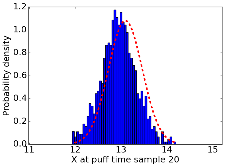
(a) X location

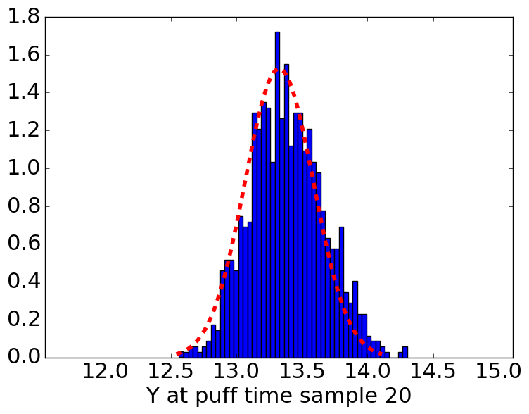
(b) Y location

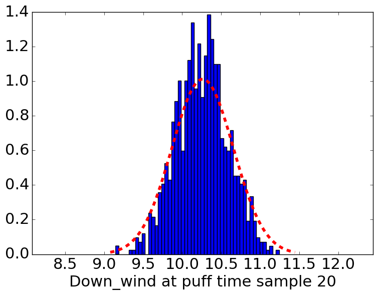
(c) Down wind

Figure 11: Example 4 (uncertainty propagation) - Histogram of $1000$ MC samples (blue) and the predicted StackedGP Gaussian distribution (red) at time step $20$

Figures 10 and 11 show the approximate predicted Gaussian distribution of the states along with the histogram of the Monte Carlo samples propagated through the StackedGP. Table 4 lists the predicted mean and standard deviation of the puff states at different time steps.

Note that even though the state equations for the location of the puff are linear, because they are emulated using a GP, which at its turn is driven by a GP model for the wind field, the distribution of the StackedGP output may depart from the Gaussian distribution. The assumption of approximating the output with a Gaussian distribution may result in biasing the mean location. The statistical significant difference between the StackedGP approximate mean propagation and its Monte Carlo estimate confirms the impact of this approximation as shown in Table 4.

Furthermore, the assumption of ignoring the correlation structure between the outputs of StackedGP may result in an artificial inflation of the uncertainty. In our simple example, this is clearly manifested in larger standard deviations for the downwind using approximate propagation as compared with the Monte Carlo estimate. This impact on uncertainty propagation might be exacerbated when more nonlinear models are used, which limits the horizon of uncertainty propagation. Obviously, the gain in computational speed combined with field measurements in the context of data assimilation may position these stacked model as real contenders for real time applications. We plan to investigate in the future the application of StackedGP to data assimilation.

6 Conclusions

A stacked model of independently trained Gaussian processes, called StackedGP, is proposed as a modeling framework in the context of model composition. This is especially of interest in environmental modeling where, e.g., model composition is used to generate large scale predictions by combining geographical interpolation models with phenomenological models developed in the lab. An approximate approach is developed to obtain estimates of the quantities of interest with quantified uncertainties. This leverages the analytical moments of a Gaussian process with uncertain inputs when squared exponential and polynomial kernels are used. The StackedGP can be extended to any number of nodes and layers and has no restriction in selecting a suitable kernel for the input nodes.

The numerical results show the utility of using StackedGP to learn from different datasets and propagate the uncertainty to quantities of interest. While it is not specifically designed to model correlations between secondary and primary responses, StackedGP can be used to enhance the prediction of primary responses by creating an intermediate layer of predictions of secondary responses. This comes with a lower computational complexity as compared with multi-output methods - and can make use of off-the-shelves Gaussian processes. While in the current paper we assume that outputs of intermediate layers are independent and resolve this using independent component analysis preprocessing, we plan to extend our derivation to account for these correlations in the next study. This will allow multi-output models to act as nodes in the proposed StackedGP.

Reference

References

- Alvarez and Lawrence (2011) Alvarez, M. A., Lawrence, N. D., 2011. Computationally efficient convolved multiple output Gaussian processes. Journal of Machine Learning Research 12 (May), 1459–1500.
- Anitescu et al. (2017) Anitescu, M., Chen, J., Stein, M. L., 2017. An Inversion-Free Estimating Equations Approach for Gaussian Process Models. Journal of Computational and Graphical Statistics 26 (1), 98–107.
- Atteia et al. (1994) Atteia, O., Dubois, J.-P., Webster, R., 1994. Geostatistical analysis of soil contamination in the swiss jura. Environmental Pollution 86 (3), 315–327.
- Bayarri et al. (2007) Bayarri, M. J., Berger, J. O., Cafeo, J., Garcia-Donato, G., Liu, F., Palomo, J., Parthasarathy, R. J., Paulo, R., Sacks, J., Walsh, D., 2007. Computer model validation with functional output. The Annals of Statistics 35 (5), 1874–1906.
-
Bhattacharya (2007)
Bhattacharya, S., 12 2007. A simulation approach to Bayesian emulation of
complex dynamic computer models. Bayesian Anal. 2 (4), 783–815.
URL http://dx.doi.org/10.1214/07-BA232 - Boyle and Frean (2005) Boyle, P., Frean, M., 2005. Dependent Gaussian processes. In: Advances in neural information processing systems. pp. 217–224.
- Candela et al. (2003) Candela, J. Q., Girard, A., Larsen, J., Rasmussen, C. E., 2003. Propagation of uncertainty in Bayesian kernel models-application to multiple-step ahead forecasting. In: Acoustics, Speech, and Signal Processing, 2003. Proceedings.(ICASSP’03). 2003 IEEE International Conference on. Vol. 2. IEEE, pp. II–701.
- Castelletti et al. (2012) Castelletti, A., Galelli, S., Ratto, M., Soncini-Sessa, R., Young, P. C., 2012. A general framework for Dynamic Emulation Modelling in environmental problems. Environmental Modelling & Software 34, 5–18.
- Castelli et al. (2015) Castelli, M., Vanneschi, L., Popovič, A., 2015. Predicting burned areas of forest fires: an artificial intelligence approach. Fire Ecology 11 (1), 106–118.
- Cheng and Sandu (2009) Cheng, H., Sandu, A., 2009. Uncertainty quantification and apportionment in air quality models using the polynomial chaos method. Environmental Modelling & Software 24 (8), 917–925.
- Conti and O’Hagan (2010) Conti, S., O’Hagan, A., 2010. Bayesian emulation of complex multi-output and dynamic computer models. Journal of Statistical Planning and Inference 140 (3), 640–651.
- Cortez and Morais (2007) Cortez, P., Morais, A. d. J. R., 2007. A data mining approach to predict forest fires using meteorological data. In: 13th Portuguese Conference on Artificial Intelligence (EPIA 2007). pp. 512–523.
- Cressie (1992) Cressie, N., 1992. Statistics for spatial data. Terra Nova 4 (5), 613–617.
- Damianou et al. (2011) Damianou, A., Titsias, M. K., Lawrence, N. D., 2011. Variational Gaussian process dynamical systems. In: Advances in Neural Information Processing Systems. pp. 2510–2518.
- Damianou and Lawrence (2013) Damianou, A. C., Lawrence, N. D., 2013. Deep Gaussian processes. In: AISTATS. pp. 207–215.
- Girard et al. (2003) Girard, A., Rasmussen, C. E., Candela, J. Q., Murray-Smith, R., 2003. Gaussian process priors with uncertain inputs-application to multiple-step ahead time series forecasting. Advances in neural information processing systems, 545–552.
- Girard et al. (2002) Girard, A., Rasmussen, C. E., Murray-Smith, R., 2002. Gaussian process priors with uncertain inputs: Multiple-step ahead prediction. University of Glasgow.
- Goovaerts (1997) Goovaerts, P., 1997. Geostatistics for natural resources evaluation. Oxford University Press on Demand.
- GPy (since 2012) GPy, since 2012. GPy: A Gaussian process framework in python. http://github.com/SheffieldML/GPy.
- Higdon (1998) Higdon, D., 1998. A process-convolution approach to modelling temperatures in the North Atlantic Ocean. Environmental and Ecological Statistics 5 (2), 173–190.
-
Higdon et al. (2008)
Higdon, D., Gattiker, J., Williams, B., Rightley, M., 2008. Computer model
calibration using high-dimensional output. Journal of the American
Statistical Association 103 (482), 570–583.
URL http://www.jstor.org/stable/27640080 - Hu and Wang (2015) Hu, J., Wang, J., 2015. Short-term wind speed prediction using empirical wavelet transform and Gaussian process regression. Energy 93, Part 2, 1456–1466.
- Jørgensen (2010) Jørgensen, S., 2010. Environmental models and simulations. In: Sydow, A. (Ed.), Environmental Systems, Vol II. Eolss Publishers, pp. 160–192.
- Katurji et al. (2015) Katurji, M., Nikolic, J., Zhong, S., Pratt, S., Yu, L., Heilman, W. E., 2015. Application of a statistical emulator to fire emission modeling. Environmental Modelling & Software 73, 254–259.
- Kennedy et al. (2002) Kennedy, M. C., O’Hagan, A., Higgins, N., 2002. Bayesian Analysis of Computer Code Outputs. In: Anderson, C. W., Barnett, V., Chatwin, P. C., El-Shaarawi, A. H. (Eds.), Quantitative Methods for Current Environmental Issues. Springer London, London, pp. 227–243.
- Konda et al. (2010) Konda, U., Singh, T., Singla, P., Scott, P., 2010. Uncertainty propagation in puff-based dispersion models using polynomial chaos. Environmental Modelling & Software 25 (12), 1608–1618.
- Letcher and Jakeman (2009) Letcher, R. A., Jakeman, A. J., 2009. Types of environmental models. In: Marquette, C. M. (Ed.), Water and Development, Vol II. Eolss Publishers, pp. 131–154.
- Li et al. (2015) Li, H., Chowdhury, A., Terejanu, G., Chanda, A., Banerjee, S., November 2015. A Stacked Gaussian Process for Predicting Geographical Incidence of Aflatoxin with Quantified Uncertainties . In: International Conference on Advances in Geographic Information Systems ACM SIGSPATIAL, Seattle, Washington.
- Lourenço and Santos (2010) Lourenço, J., Santos, P., 2010. Short term load forecasting using Gaussian process models. Proceedings of Instituto de Engenharia de Sistemas e Computadores de Coimbra.
- Machac et al. (2016) Machac, D., Reichert, P., Rieckermann, J., Albert, C., 2016. Fast mechanism-based emulator of a slow urban hydrodynamic drainage simulator. Environmental Modelling & Software 78, 54–67.
- Meier et al. (2014) Meier, F., Hennig, P., Schaal, S., 2014. Incremental local Gaussian regression. In: Advances in Neural Information Processing Systems. pp. 972–980.
- Moonen and Allegrini (2015) Moonen, P., Allegrini, J., 2015. Employing statistical model emulation as a surrogate for CFD. Environmental Modelling & Software 72, 77–91.
- Neumann et al. (2009) Neumann, M., Kersting, K., Xu, Z., Schulz, D., 2009. Stacked Gaussian process learning. In: 2009 Ninth IEEE International Conference on Data Mining. IEEE, pp. 387–396.
- Nielsen et al. (1999) Nielsen, S., Deme, S., Mikkelsen, T., 1999. Description of the Atmospheric Dispersion Module RIMPUFF. Tech. Rep. RODOS(WG2)-TN(98)-02, Riso National Laboratory, P.O.Box 49, DK-4000 Roskilde, Denmark.
- O’Hagan (2006) O’Hagan, A., 2006. Bayesian analysis of computer code outputs: A tutorial. Reliability Engineering & System Safety 91 (10), 1290–1300.
- Rasmussen (1997) Rasmussen, C. E., 1997. Evaluation of Gaussian processes and other methods for non-linear regression. Ph.D. thesis, Toronto, Ont., Canada, Canada, aAINQ28300.
- Rasmussen and Williams (2005) Rasmussen, C. E., Williams, C. K. I., 2005. Gaussian Processes for Machine Learning. MIT press.
- Reddy et al. (2006) Reddy, K. V. U., Singh, T., Cheng, Y., Scott, P. D., July 2006. Data assimilation for dispersion models. In: 2006 9th International Conference on Information Fusion. pp. 1–8.
- Reggente et al. (2014) Reggente, M., Peters, J., Theunis, J., Van Poppel, M., Rademaker, M., Kumar, P., De Baets, B., 2014. Prediction of ultrafine particle number concentrations in urban environments by means of Gaussian process regression based on measurements of oxides of nitrogen. Environmental Modelling & Software 61, 135–150.
- Seeger et al. (2005) Seeger, M., Teh, Y.-W., Jordan, M., 2005. Semiparametric latent factor models. Tech. rep.
- Snelson and Ghahramani (2006) Snelson, E., Ghahramani, Z., 2006. Sparse Gaussian processes using pseudo-inputs. Advances in neural information processing systems 18, 1257.
- Snelson (2007) Snelson, E. L., 2007. Flexible and efficient Gaussian process models for machine learning. Ph.D. thesis, Citeseer.
- Sun et al. (2014) Sun, A. Y., Wang, D., Xu, X., 2014. Monthly streamflow forecasting using Gaussian Process Regression. Journal of Hydrology 511, 72–81.
- Sykes et al. (2006) Sykes, R., Parker, S., Henn, D., Chowdhury, B., 2006. SCIPUFF Version 2.2 Technical Documentation. Tech. Rep. 729, L-3 Titan Corporation.
- Taylor and Alexander (2006) Taylor, S. W., Alexander, M. E., 2006. Science, technology, and human factors in fire danger rating: the canadian experience. International Journal of Wildland Fire 15 (1), 121–135.
- Terejanu et al. (2008) Terejanu, G., Cheng, Y., Singh, T., Scott, P. D., November 2008. Comparison of SCIPUFF plume prediction with particle filter assimilated prediction for Dipole 26 data. In: Chemical and Biological Defense Physical Science and Technology Conference, New Orleans.
- Terejanu et al. (2007) Terejanu, G., Singh, T., Scott, P. D., July 2007. Unscented Kalman filter/smoother for a CBRN puff-based dispersion model. In: 11th International Conference on Information Fusion, Quebec City, Canada.
- Tokmakian et al. (2012) Tokmakian, R., Challenor, P., Andrianakis, Y., 2012. On the Use of Emulators with Extreme and Highly Nonlinear Geophysical Simulators. Journal of Atmospheric and Oceanic Technology 29 (11), 1704–1715.
- Van Wagner et al. (1985) Van Wagner, C., Pickett, T., et al., 1985. Equations and FORTRAN program for the Canadian forest fire weather index system. Vol. 33.
- Wang et al. (2014) Wang, Y., Ocampo-Martínez, C., Puig, V., Quevedo, J., 2014. Gaussian-process-based demand forecasting for predictive control of drinking water networks. In: International Conference on Critical Information Infrastructures Security. Springer, pp. 69–80.
- Webster et al. (1994) Webster, R., Atteia, O., DUBOIS, J.-P., 1994. Coregionalization of trace metals in the soil in the swiss jura. European Journal of Soil Science 45 (2), 205–218.
- Williams (1998) Williams, C. K., 1998. Prediction with Gaussian processes: From linear regression to linear prediction and beyond. In: Learning in graphical models. Springer, pp. 599–621.
- Williams and Rasmussen (1996) Williams, C. K. I., Rasmussen, C. E., 1996. Gaussian processes for regression. In: Advances in Neural Information Processing Systems. Vol. 8. MIT press, pp. 514–520.
- Wilson et al. (2012) Wilson, A. G., Knowles, D. A., Ghahramani, Z., June 2012. Gaussian process regression networks. In: Langford, J., Pineau, J. (Eds.), Proceedings of the 29th International Conference on Machine Learning (ICML). Omnipress, Edinburgh.