Spectral and timing properties of IGR J00291+5934 during its 2015 outburst

Abstract

We report on the spectral and timing properties of the accreting millisecond X-ray pulsar IGR J00291$+$5934 observed by XMM-Newton and NuSTAR during its 2015 outburst. The source is in a hard state dominated at high energies by a comptonization of soft photons ($\sim 0.9$ keV) by an electron population with kT${}_{e}\sim 30$ keV, and at lower energies by a blackbody component with kT$\sim 0.5$ keV. A moderately broad, neutral Fe emission line and four narrow absorption lines are also found. By investigating the pulse phase evolution, we derived the best-fitting orbital solution for the 2015 outburst. Comparing the updated ephemeris with those of the previous outbursts, we set a $3\sigma$ confidence level interval $-6.6\times 10^{-13}$ s/s $<\dot{P}_{orb}<6.5\times 10^{-13}$ s/s on the orbital period derivative. Moreover, we investigated the pulse profile dependence on energy finding a peculiar behaviour of the pulse fractional amplitude and lags as a function of energy. We performed a phase-resolved spectroscopy showing that the blackbody component tracks remarkably well the pulse-profile, indicating that this component resides at the neutron star surface (hot-spot).

1 Introduction

IGR J00291$+$5934 is a transient low mass X-ray binary system (LMXB) observed in outburst for the first time in 2004 (e.g. Eckert et al., 2004; Galloway et al., 2005). After a peculiar double outburst in 2008 (see e.g. Patruno, 2010; Papitto et al., 2011; Hartman et al., 2011), the source went in outburst again, for the fourth time, in 2015. This last outburst was detected by Swift/BAT on July 23rd 2015 (Sanna et al., 2015), and lasted approximately 20 days. With its $\sim 599$ Hz spin frequency, IGR J00291$+$5934 is the fastest objects belonging to the class of systems known as accreting millisecond X-ray pulsars (AMXP; see Burderi & Di Salvo, 2013; Patruno & Watts, 2012, for some recent reviews). AMXPs are fast rotating neutron stars (NS) that accrete matter via Roche-lobe overflow from an evolved sub-Solar companion star. The extremely fast spin periods observed in AMXPs are the result of a long-term accretion process in which an old slow-spinning radio-pulsar has continuously gained angular momentum (recycling scenario; Alpar et al., 1982). The link between radio millisecond pulsars and AMXPs has been recently confirmed by the radio and X-ray swinging behaviour of AMXPs IGR J18245$-$2452 (Papitto et al., 2013), as well as for the low luminosity systems PSR J0023+0038 (Stappers et al., 2014; Archibald et al., 2015) and XSS J12270-4859 (Bassa et al., 2014; Papitto et al., 2015).

Timing analysis of the X-ray pulsations revealed a sinusoidal modulation with period of $\sim 2.5$ hr and a corresponding projected semi-major axis of $a\,sin(i)\sim 65$ lt-ms (see e.g. Galloway et al., 2005; Patruno, 2010; Papitto et al., 2011; Hartman et al., 2011). The NS mass function implies a minimum companion mass of 0.039 M_⊙ (assuming a 1.4 M_⊙ NS). An upper limit of 0.16 M_⊙ for the companion star has been set considering an isotropic a priori distribution of binary system inclinations (Galloway et al., 2005). Linares et al. (2007) identified flat-top noise and two quasi-periodic oscillations (QPOs), both at low frequencies (0.01–0.1 Hz), in the source power density spectrum (PDS) obtained by the Rossi X-ray Timing Explorer (RXTE) data. While the timing properties of the source have been well studied, the spectral properties are still poorly known. Falanga et al. (2005) found that the source can be described, in the 5-200 keV energy range, by thermal Comptonization with an electron temperature >50 keV. During the 2015 outburst, the source showed for the first time a type-I X-ray burst (Bozzo et al., 2015), probably ignited in a pure He layer.

Here, we focus on the spectral and temporal properties of IGR J00291$+$5934 by analysing high quality, simultaneous XMM-Newton and NuSTAR observations of the latest outburst of IGR J00291$+$5934.

2 Observations and data reduction

We analysed two simultaneous XMM-Newton and NuSTAR observations of the 2015 outburst of IGR J00291$+$5934 performed on 2015 July 28 (Obs.ID. 0790181401 and 90101010002, respectively) during the descent phase of the outburst. No type-I bursts were detected.

The EPIC-pn (hereafter PN) and EPIC-MOS2 (hereafter MOS2) cameras were operated in TIMING mode (for a total exposure time of $\sim 72$ and $\sim 86$ ks, respectively, while the RGS instrument was observed in spectroscopy mode for a total exposure of $\sim 86$ ks. We excluded the EPIC-MOS1 (operated in IMAGING mode) from the analysis because highly piled-up. We extracted the XMM-Newton data using the Science Analysis Software (SAS) v. 15.0.0 with the up-to-date calibration files, and performing the standard reduction pipeline RDPHA (e.g. Pintore et al., 2014, see also XMM-CAL-SRN-0312). PN and MOS2 source events were selected in the range 0.3$-$10.0 keV and for RAWX=[32:44] and RAWX=[291:322], screening events with pattern$\leq$4 and $\leq$12, respectively. Background was extracted in a RAWX region with small source photons contamination.

We extracted PN and MOS2 energy spectra (source and background) setting ‘FLAG=0’ to retain only events optimally calibrated for spectral analysis. RGS were extracted adopting the rgsproc pipeline, selecting only first order spectra. PN, MOS2 and RGS spectra were binned in order to have at least 100 counts per bin.

NuSTAR observed IGR J00291$+$5934 simultaneously with XMM-Newton. The observation was reduced performing standard screening and filtering of the events by means of the NuSTAR data analysis software (nustardas) version 1.5.1, for an exposure time of roughly $\sim$40ks for the two instruments. We extracted source and background events from circular regions of 80” and 120” radius, respectively. Source spectra, response files and light curves for each instrument were generated using the nuproducts pipeline.

Solar System barycentre corrections were applied to PN and NuSTAR photon arrival times with the barycen and barycorr tools (using DE-405 solar system ephemeris), respectively. We adopted the source coordinates obtained observing the optical counterpart of the source (Torres et al., 2008), and reported in Tab. 2.

3 Data analysis

3.1 Spectral analysis

The XMM-Newton and NuSTAR light-curves of IGR J00291$+$5934 shows rapid variability on time-scales between tens and few hundreds seconds, compatible with the low-frequency QPO reported by Linares et al. (2007) and Ferrigno et al. (2016), and accompanied by spectral variability. Fig. 1 shows a zoom-in of the hardness ratio during the XMM-Newton observation. We suggest the presence of different spectral states as the result of rapid changes in the mechanism generating the hard and the soft emission. Alternatively, the source could be experiencing continuous dipping activity, although quite unlikely as dips usually occur for system seen at high inclination angles ($>70^{\circ}$ Frank et al., 1987). Instead Torres et al. (2008) suggested an orbital inclination $22^{\circ}<i<32^{\circ}$, obtained from the analysis of the H-$\alpha$ emission line profile. Moreover, if the frequency of the variability is associated with the Keplerian velocity of a cusp in the outer disc edge, the latter should be at a distance of $\sim 0.11$ lt-s which is at least a factor of 1.7 larger than the projected NS semi-major axis assuming an inclination angle $i\leq 65^{\circ}$ (see Table 2). Although very intriguing, the study of this behaviour is beyond the scope of this paper and it has been instead investigated in a companion paper (Ferrigno et al., 2016). Here, we focus on the average properties of IGR J00291$+$5934.

Figure 1: Soft (0.3–1.5 keV), hard (1.5–10 keV) and corresponding hardness ratio (hard/soft) PN light-curve of IGR J00291$+$5934 .

We fitted the XMM-Newton and NuSTAR average broadband spectrum in the energy range 0.4–10 keV and 3.0–70 keV, respectively, adopting a continuum model based on an absorbed nthcomp and a bbody component. For the absorber we adopted the tbabs model with the abundances of Anders & Grevesse (1989). In addition, we modelled the Au instrumental edge ($\sim$2.2 keV) with a gaussian component. Interestingly, we observed a broad emission at $\sim 6.4$ keV (likely associated to the Fe), fitted with a gaussian.

We found the source in a hard state and we estimated a total unabsorbed source flux in the 0.3–70 keV energy range of $(3.37\pm 0.01)\times 10^{-10}$ erg cm^-2 s^-1. The spectral parameters are characterised by an $N_{\rm H}$ of $(0.226\pm 0.007)\times 10^{22}$ cm^-2 and with the hard energy emission dominated by Comptonization ($\Gamma=1.735\pm 0.008$) produced by an electron population with temperature of $27.9_{-3.2}^{+4.8}$ keV. The bbody temperature ($0.50\pm 0.02$ keV) is not compatible with the temperature of the seed photons of the hard component ($0.85\pm 0.05$ keV). Moreover, we note that the PN spectrum shows a different slope above $\sim 7$ keV, in comparison with the MOS2 and the NuSTAR spectra. This discrepancy is likely the result of a still uncertain cross-calibration between the PN operated in timing mode and the other instruments. We corrected for this issue by linking the photon index of the NuSTAR and MOS2 spectra and by letting this parameter free to vary with respect to the PN spectrum. As a result we obtained two photon indexes differing by $\sim 6-7\%$ (i.e. $1.62\pm 0.02$ vs $1.734\pm 0.007$). However, the reduced $\chi^{2}$ of the best-fit is still quite high ($\chi^{2}/\text{d.o.f.}=3321.86/2738$). Hence, to take into account the large value of the reduced $\chi^{2}$, we added a systematic uncertainty of 0.25$\%$ to the spectral data. We note that, hereafter, the uncertainties will be reported at 90% confidence level for each parameter of interest (see table 1).

We also observed an Fe emission line at an energy of $6.37\pm 0.04$ keV with a $\sigma$ of $80\pm$70 eV and an equivalent width of $\sim$20 eV. To further investigate the origin the feature, we substituted the gaussian with a relativistic blurred reflection emission line (diskline; Fabian et al. 1989). We fixed the emissivity index and the outer disc radius to -2.7 and $10^{5}$ R_g, respectively, as the fit was insensitive to these parameters. The best-fit ($\chi^{2}/\text{d.o.f.}=2702.79/2737$) gives an inner disc radius poorly constrained ($43^{+910}_{-18}$ R_g) and an inclination angle highly unconstrained (Tab. 1). These results confirm the presence of the reflection feature but do not allow us to precisely locate the region of origin in the disc. We also applied a self-consistent reflection model rfxconv (Kolehmainen et al., 2011) convolved with the relativistic kernel rdblur. We obtained a best-fit ($\chi^{2}/\text{d.o.f.}=2708.45/2737$) which was statistically worse with respect to the previous model, which gives a very low ionisation parameter log$\xi=1.0\pm 0.13$ and a small reflection fraction $0.04^{+0.03}_{-0.01}$. The parameters of the component rdblur were highly unconstrained, therefore, we fixed the outer radius and emissivity index to $R_{out}=10^{5}$ R_g and $\beta=-2.7$, respectively. From the fit we found a poorly constrained source inclination ($36^{+30}_{-16}$ degrees). Moreover, we set an upper limit to the inner radius (R${}_{in}>130$ R_g), which is consistent with the large radius expected by the 0.1 keV width of the line.

Finally, we found evidence of some statistically significant absorption lines. In particular, a narrow absorption feature at $7.04\pm 0.04$ keV ($\Delta\chi^{2}=38.1$ for 2 d.o.f., corresponding to F-test probability of chance improvement, $p=1.2\times 10^{-7}$), possibly identified with the Fe XXVI K_α transition blue-shifted with v $\sim 0.01c$, an absorption lines at $0.756\pm 0.002$ keV ($\Delta\chi^{2}=19.3$ for 2 d.o.f., $p=3.3\times 10^{-4}$) which might be likely associated to O VII or VIII. We also found a marginally significant absorption line at $0.872\pm 0.002$ keV which might be associated to Ne I ($\Delta\chi^{2}=12.23$ for 2 d.o.f., $p=6.2\times 10^{-3}$) and, if realistic, it would be blue-shifted by 0.02-0.03 c. The final best-fit, with these lines and in the case of Fe emission line fitted with a gaussian model, gives $\chi^{2}/\text{d.o.f.}=2655.67/2730$ and it is shown in Fig. 2.

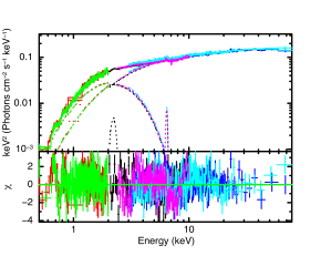
Figure 2: Top-panel: X-ray spectrum of IGR J00291$+$5934 observed by the RGS1 (red points), RGS2 (green points), PN (black points), MOS1 (magenta points), NuSTAR FMPA (blue points), NuSTAR FMPB (cyan points) and the best-fitting model tbabs*(gaussian+gaussian+bbody+nthcomp). Bottom-panel: Residuals with respect to the best fitting model. The data have been visually rebinned.

Model	Component	(1)	(2)
TBabs	nH ($10^{22}$)	$0.237^{+0.01}_{-0.009}$	$0.237^{+0.008}_{-0.007}$
bbody	kT (keV)	$0.5^{+0.02}_{-0.02}$
	norm (10-4)	$6.8^{+0.5}_{-0.6}$
nthComp	Gamma (pn)	$1.62^{+0.02}_{-0.02}$
	Gamma (MOS, NuSTAR)	$1.734^{+0.007}_{-0.006}$
	kTe (keV)	$27.9^{+4.8}_{-3.2}$
	kTbb (keV)	$0.85^{+0.05}_{-0.06}$
	norm (10-3)	$6.5^{+0.9}_{-0.7}$
gaussian	LineE (keV)	$6.37^{+0.04}_{-0.04}$	-
	$\sigma$ (keV)	$0.08^{+0.06}_{-0.08}$	-
	norm (10-5)	$4.3^{+1.3}_{-1.2}$
Diskline	LineE (keV)	-	$6.46^{+0.08}_{-0.06}$
	Betor10	-	-2.7 (frozen)
	Rin(M)	-	$43^{+910}_{-18}$
	Rout(M)(105)		1.0 (frozen)
	Incl(deg)	-	unconstrained
	norm(10-5)	-	$4.3^{+1.2}_{-1.2}$
$\chi^{2}/\text{d.o.f.}$		2702.72/2738	2702.79/2737

Table 1: Best fit spectral parameters obtained with the absorbed continuum bbody+nthcomp model, plus either a gaussian (model 1) or diskline (model 2) component for the Fe emission line. Uncertainties are at 90$\%$ for each parameter of interest.

3.2 Timing analysis

Following the procedure described in Burderi et al. (2007), we corrected the photon time of arrivals of both the PN and the NuSTAR datasets for the delays caused by the binary motion applying the orbital parameters reported by Papitto et al. (2011, see also ) for the latest outburst of the source on September 2008. We then performed an epoch-folding search of the whole PN and NuSTAR observations around the spin frequency of the September 2008 outburst (Papitto et al., 2011). We found evidence of X-ray pulsation in both the PN and NuSTAR observations. The PN average pulse profile is well fitted by two sinusoids with fractional amplitude of 13.45(7)% and 0.58(7)%, for the fundamental and the first harmonic, respectively. The NuSTAR pulse profile is well described by a single sinusoid with fractional amplitude of 11.2(2)%.

We created pulse phase delays computed over time intervals of approximately 300s for the PN observation and 500s for the NuSTAR observation, epoch-folding the intervals at the mean spin frequency values for each instrument. Although strictly simultaneous, no phase-connected timing analysis was applicable due to the presence of a time drift on the internal clock on NuSTAR (Madsen et al., 2015), which affects the observed coherent signal making the spin frequency value significantly different compared to the XMM-Newton value. It can be shown that the latter spurious phase delay only marginally affects the phase delays induced by the orbital motion (see, e.g. Riggio et al., 2007, for similar phenomena), therefore we were still able to investigate the orbital ephemerides combining the two observations. We fitted the pulse phase delays time evolution with the following models:

$$\begin{cases}\Delta\phi_{NuStar}(t)=\sum\limits_{n=0}^{4}\frac{C_{n}}{n!}(t-T_{0})^{n}+R_{orb}(t)\\ \Delta\phi_{XMM}(t)=\sum\limits_{n=0}^{2}\frac{D_{n}}{n!}(t-T_{0})^{n}+R_{orb}(t)\end{cases}$$ (1)

where the first element represents a polynomial function used to model the phase variations in each dataset. Additionally, the component $R_{orb}(t)$ represents the Roemer delay component, where the differential correction on the orbital parameters are determined combining the two dataset. If a new set of orbital parameters is found, we repeated the process described above until no significant differential corrections were found. We reported the best-fit parameters in Table 2, while in Fig. 3 we showed the pulse phase delays of the two observations with the best-fitting models (top panel), and the residuals with respect to the best-fitting model.

We estimated the systematic uncertainty induced on the spin frequency correction $\Delta\nu_{0}$ because of the positional uncertainties of the source using the approximated expression $\sigma_{\nu_{pos}}\leq\nu_{0}\,y\,\sigma_{\gamma}(1+\sin^{2}\beta)^{1/2}2\pi/P_{\oplus}$, where $y=r_{E}/c$ is the semi-major axis of the orbit of the Earth in light-seconds, $P_{\oplus}$ is the Earth orbital period, and $\sigma_{\gamma}$ is the positional error circle of the residuals (for more details see e.g. Lyne & Graham-Smith, 1990; Burderi et al., 2007). Adopting the positional uncertainties reported by Torres et al. (2008), we estimate $\sigma_{\nu_{pos}}\leq 5\times 10^{-8}$ Hz. We added in quadrature the systematic uncertainty to the statistical errors of $\nu_{0}$ reported in Table 2.

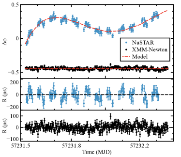
Figure 3: Top panel - Pulse phase delays as a function of time computed by epoch-folding 300 second data intervals of the XMM-Newton observations and 500 second data intervals of the NuSTAR observation. Red dotted line represents the best-fit model (see text for more details). Middle panel - Residuals in $\mu s$ of the NuSTAR data with respect to the best-fitting orbital solution. Bottom panel - Residuals in $\mu s$ of the XMM-Newton data with respect to the best-fitting orbital solution.

Finally, we explored the dependence of the pulse profile fractional amplitude and time lags (defined as the phase shift of the fundamental harmonic of the pulse profile in different energy bands) as a function of energy, dividing the energy range between 0.3 keV to 10 keV into 21 intervals, and the energy range between 1.6 keV and 80 keV into 13 intervals, for XMM-Newton and NuSTAR, respectively. Since the two dataset are not phase connected, we calculated the time lags using different reference profiles. For display purposes only, for both dataset we set the reference at around 7 keV. In Fig. 4 we reported the dependence of the time lags (top panel) and the fractional amplitude (bottom panel) as a function of energy for the XMM-Newton and NuSTAR pulse profiles, represented with black dots and red squares, respectively.

Parameters	XMM	NuSTAR
R.A. (J2000)	$00^{h}29^{m}3.05^{s}$
DEC (J2000)	$59^{\circ}34^{m}18.93^{s}$
$P_{orb}$ (s)	8844.08(2)
$x$ (lt-s)	0.0649905(24)
$T_{NOD}$ (MJD)	57231.437581(3)
e	<$2\times 10^{-4}$
$\nu_{0}$ (Hz)	598.8921309(2)	598.892168(2)
$\dot{\nu}_{0}$ (Hz/s)	$3(5)\times 10^{-12}$	-
$T_{ref}$ (MJD)	57231.5a
$\chi^{2}_{\nu}$/d.o.f.	491.5/348

Table 2: Orbital parameters and spin frequency of IGR J00291$+$5934 obtained from the analysis of the XMM-Newton and NuSTAR observations of the source. Errors are at 1$\sigma$ confidence level. Uncertainties are also scaled by a factor $\sqrt{\chi^{2}_{red}}$ to take into account the large value of the reduced $\chi^{2}$. The reported X-ray position of the source has a pointing uncertainty of 0.05^′′ (see e.g. Torres et al., 2008).^a Timing solution reference epoch.

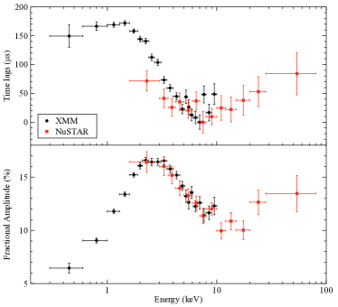
Figure 4: Top panel - Time lags in $\mu s$ evolution as a function of energy obtained from the XMM-Newton and NuSTAR observations reported with black dots and red squares, respectively. For display purpose only the reference pulse profiles of the two datasets has been set around 7 keV. Bottom panel - Evolution of the pulse fractional amplitude for the two datasets. The colour coding has been kept fixed between the panels.

4 Phase-resolved spectroscopy

After correcting the photon times of arrival for the orbital ephemerides reported in Table 2, we performed a phase-resolved spectroscopy with the aim to study the evolution of the spectral components as a function of the NS spin phase. Given the previously described spectral discrepancy between the detectors and the timing issues reported for NuSTAR, we decided to focus on the PN data only. We split the pulse profile in 10 phase bins of equal size and for each phase interval we extracted the corresponding PN spectrum. We fitted simultaneously the 10 spectra in the energy range 2.0–10 keV. In analogy with the best-fit model of the average broadband spectrum, we fitted the continuum with the model bbodyrad+nthcomp. Moreover, we included two broad emission features to take into account the Au instrumental feature at 2.2 keV and the Iron line. Given the lack of coverage below 2 keV, we fixed the hydrogen column density to the value $0.237\times 10^{22}$ cm^-2 and the kT_e temperature of the comptonisation component (nthcomp) to 27.8 keV (i.e., the best-fit values of the averaged spectrum). We note that the high energy component was only marginally changing among the spectra, therefore we decided to link together the parameters of the 10 spectra. On the other hand, the blackbody component clearly showed variability correlated with the spin pulse profile (see Table 3 and Fig. 5), with variations of 0.2 keV. In particular we found that the temperature profile is slightly offset with respect to the pulse-profile, with the highest/lowest blackbody temperature lagging by $\sim$0.1 in phase the peak/bottom of the sinusoidal pulse-profile. A similar result is also found for the corresponding emitting radius in the opposite direction, so that the black-body bolometric flux remain aligned with the pulse profile, with the large uncertainties. These results allow us to unequivocally associate the soft component to the NS.

Model	Component	(1)	(2)	(3)	(4)	(5)	(6)	(7)	(8)	(9)	(10)
TBabs	nH ($10^{22}$)	0.226 (fixed)
bbodyrad	kT (keV)	$0.63_{-0.03}^{+0.03}$	$0.62_{-0.02}^{+0.02}$	$0.63_{-0.02}^{+0.02}$	$0.58_{-0.01}^{+0.03}$	$0.56_{-0.03}^{+0.03}$	$0.51_{-0.04}^{+0.04}$	$0.59_{-0.05}^{+0.05}$	$0.70_{-0.06}^{+0.06}$	$0.71_{-0.05}^{+0.04}$	$0.70_{-0.03}^{+0.03}$
	norm	$156.6_{-23.5}^{+28.2}$	$195.0_{-25.7}^{+30.1}$	$189.5_{-24.3}^{+28.4}$	$224.9_{-35.5}^{+44.3}$	$235.5_{-41.5}^{+53.2}$	$264.8_{-69.1}^{+106.5}$	$93.2_{-26.1}^{+40.3}$	$49.5_{-13.2}^{+17.8}$	$61.1_{-13.4}^{+16.6}$	$90.8_{-15.0}^{+17.6}$
nthComp	$\Gamma$	$1.459^{+0.02}_{-0.009}$
	kTe (keV)	28.8 (fixed)
	kTbb (keV)	$0.09^{+0.18}_{-0.09}$
	norm	$0.29_{-0.06}^{+0.01}$	$0.29_{-0.06}^{+0.01}$	$0.28_{-0.06}^{+0.01}$	$0.26_{-0.05}^{+0.01}$	$0.24_{-0.05}^{+0.005}$	$0.232_{-0.05}^{+0.004}$	$0.233_{-0.05}^{+0.009}$	$0.25_{-0.05}^{+0.01}$	$0.27_{-0.06}^{+0.01}$	$0.28_{-0.06}^{+0.01}$
gaussian	LineE(keV)	$6.47^{+0.04}_{-0.04}$
	Sigma(keV)	$0.13^{+0.04}_{-0.04}$
	norm(10-4)	$5.1^{+1.0}_{-1.0}$
gaussian	LineE(keV)	$2.240^{+0.01}_{-0.006}$
	Sigma(keV)	$0.04^{+0.02}_{-0.03}$
	norm(10-3)	$1.2^{+0.3}_{-0.3}$
	$\chi^{2}/\text{d.o.f.}$	976.42/957

Table 3: Best fit spectral parameters obtained with an absorbed continuum bbody+nthcomp model, plus either two gaussian components for the Fe emission line and the instrumental Au calibration residual. Uncertainties are expressed at a 90% confidence level

Figure 5: Phase-resolved spectral analysis as reported in Table 3. In the top panel, the pulse profile in the 0.3–10 keV energy band, in the second panel the unabsorbed 0.3–10 keV flux (in erg cm² s^-1), in the third and fourth panels the bbodyrad temperature and the corresponding radius, and in the bottom panel the blackbody flux estimated as $r^{2}kT^{4}$ and expressed in arbitrary units (a.u.). Uncertainties are expressed at a 90% confidence level.

5 Discussion

IGR J00291$+$5934 shows a hard spectrum dominated by comptonization as typically observed in other AMXPs (e.g. Papitto et al., 2009; Patruno et al., 2010). The region producing the seed photons can be estimated by using the relations proposed by in ’t Zand et al. (1999, $R_{seed}=3\times 10^{4}\,d\sqrt{f_{bol}/(1+y)}/kT_{bb}^{2}$), where $f_{bol}$ is the bolometric flux of the nthcomp component and y is the Compton parameter. Assuming a distance of 4 kpc (Galloway et al., 2005), we inferred a region size of $1.4\,d_{4kpc}$ km. The soft component shows instead a temperature of 0.5 keV, not compatible with the seed photons temperature, and corresponding to an emission region of $0.5\,d_{4kpc}$ km. The size of this region is almost a factor of three smaller compared with the seed photons, however, both are likely incompatible with the inner radius of the accretion disc. Our interpretations are quite consistent with the findings of Paizis et al. (2005) which performed a spectral analysis on Chandra and RXTE data of the fainter end of the 2005 source outburst.

Remarkably, the phase-resolved spectroscopy analysis allowed us to clearly associate the blackbody component with the NS, as we found that the variations in temperature are related to the pulse evolution. We associated the blackbody component with the hot-spot on the NS surface, and its radius and temperature track well the evolution of the pulse profile, indicating that the temperature is higher or lower when the pulse points toward us or in opposition to us. We note that the delay of $\sim$0.1 in phase of the temperature with respect to the pulse-profile may be caused by comptonization effects of the hot-spot thermal emission. Alternatively, a combination of temperature gradient in the hot-spot emission region and inclination angle of the accretion column with respect to the line of sight could be responsible for the observed phase misalignment. More observations with higher statistics are required to further investigate the spectral properties of the source as function of the spin pulse phase in order to confirm or disprove the proposed scenario.

The presence of a neutral Fe emission line only weakly broadened (0.1 keV, i.e. $\sim$0.01c assuming Doppler broadening) combined with the lack of statistically significant improvement when applying a self-consistent relativistically smeared reflection component to the data do not robustly support a reflection originated from the inner regions of the disc. Nonetheless, we cannot discard the possibility of a line originated by reflection off of hard photons in the outer disc. However, since persistent X-ray pulsations require a magnetospheric radius smaller than the co-rotation radius (of the order of 24 km for IGR J00291$+$5934), it needs to be explained the lack of the reflection component in this region. We suggest two possible scenarios to explain such findings: i) if the line is produced by reflection off of hard photons by the accretion disc, the self-consistent model suggest a weakly ionised disc, consistent with the presence of neutral iron, but produced very far from the NS ($>100$ R_g) and this may be compatible with the phenomenology of systems accreting at low Eddington rates ($<10^{-2}$ L${}_{\text{edd}}$, see Degenaar et al., 2016, for more details on the topic; see also D’Aì et al. 2010, Di Salvo et al. 2015). We suggest that the lack of inner disc reflection may be due to either a continuum inefficient to illuminate the disc as a beamed emission of the direct comptonisation component inclined with respect to the accretion disk, or the inner disc may eject outflows (in the form of winds) for local violations of the Eddington limit (e.g. Poutanen et al., 2007), that might also be responsible for the absorption lines observed in the system. This could cause changes in the amount of mass transferred onto the NS giving raise to the observed variability on timescales of $\sim 100$s, in analogy with the Galactic BH candidate GRS 1915+105 and to its observed “heartbeat” on short-timescales and also outflowing wind (e.g. Neilsen et al., 2012). However, a caveat on this interpretation may be the luminosity of IGR J00291$+$5934, which is orders of magnitude lower than that of GRS 1915+105, hence making difficult to explain how such outflows are produced. However, similar "heartbeats" are also observed in the BH candidate IGR J17091-3624 (Altamirano et al., 2011) which may have a luminosity orders of magnitude lower than that of GRS 1915+105, hence allowing not to exclude such processes also in IGR J00291+5934. ii) Alternatively, the iron line may be produced in a corona and broadened either by velocity dispersions (of the order of 0.01 c) in the corona or by Compton scattering in a moderately optically thick and relatively cold medium; in the latter case also the mechanism proposed by Laurent & Titarchuk (2007) of a Compton down-scattering produced by a narrow wind shell outflowing at mildly relativistic speed may play a role, although in this case a significant red-wing of the line is also expected.

From the timing analysis, we detected X-ray pulsations at the spin frequency period of IGR J00291$+$5934 with an average fractional amplitude of 13% and 11% for XMM-Newton and NuSTAR, respectively. From the evolution of the pulse phase delays obtained from the two datasets of the 2015 outburst, we obtained an updated timing solution for the source. The new set of orbital parameters is compatible within the errors with the previous timing solution obtained from the analysis of the 2004 (Galloway et al., 2005; Falanga et al., 2005; Burderi et al., 2007) and 2008 outbursts (Patruno, 2010; Papitto et al., 2011; Hartman et al., 2011). Combining the measurements of the time of passage of the NS at the ascending node ($T_{NOD}$) for each observed outburst we computed the delays $\Delta T_{NOD}$ as a function of time. $\Delta T_{NOD}$ is obtained by subtracting from each measurement the $T_{NOD_{pred}}=T_{NOD_{ref}}+NP_{orb_{ref}}$ predicted by a constant orbital period model (see e.g. Di Salvo et al., 2008; Burderi et al., 2009; Sanna et al., 2016) adopting the orbital period $P_{orb_{ref}}=8844.079(1)$ s and the time of passage of the NS at the ascending node $T_{NOD_{ref}}=53345.1619264(5)$ MJD of the first observed outburst of the source in 2004 reported by Papitto et al. (2011). The integer $N$ represents the closest integer number of orbital cycles elapsed between two different $T_{NOD}$ observed. We fitted the delays with the expression $\Delta T_{NOD}=\delta T_{NOD_{ref}}+N\,\delta P_{orb_{ref}}+0.5\,N^{2}\,\dot{P}_{orb}P_{orb_{ref}}$, where $\dot{P}_{orb}$ represents the orbital period derivative. We obtained the best-fit for $\delta T_{NOD_{ref}}=-0.0005(4)\times 10^{-2}$ MJD, $\delta P_{orb_{ref}}=2.27(4)\times 10^{-3}$ s and $\dot{P}_{orb}=-0.7(2.2)\times 10^{-13}$ s/s, with $\chi^{2}=0.008$ for 1 degree of freedom. Fig. 6 shows $\Delta T_{NOD}$ values for the observed outbursts as a function of the number of orbital cycles elapsed from the reference epoch (top panel) as well as the residuals with respect to the best-fitting model described above (bottom panel). We note that the reduced $\chi^{2}$ is significantly smaller compared with the expected value one, likely indicating that the testing of the model would require more precise data. However, the probability to obtain a $\chi^{2}$ smaller than the observed is $\sim 7\%$, marginally above the conventionally accepted significant threshold of 5$\%$ (see e.g. Bevington & Robinson, 2003).

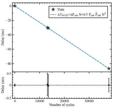
Figure 6: Top panel - Time delays of the NS time of passage from the ascending node for each of the observed outbursts of IGR J00291$+$5934. The cyan dashed line represents the best-fitting parabola used to model the data. Bottom panel - Residuals in seconds of the time delays with respect to the best-fitting timing solution.

From the fit, we cannot constrain both the correction on the time of passage from the ascending node and the orbital period derivative. However, we find a significant correction on the orbital period at the reference time (2004 outburst) finding $P_{orb}=8844.07673(3)$ s, in agreement with the estimate reported by Hartman et al. (2011). Moreover, we note that the timing solution and our new estimate of the orbital period found from our analysis are fully consistent, within uncertainties, with those obtained from the analysis of the INTEGRAL data (De Falco et al., 2016). For the orbital period we can at least define the $3\sigma$ confidence level interval $-6.6\times 10^{-13}$ s/s $<\dot{P}_{orb}<6.5\times 10^{-13}$ s/s (compatible within errors with the estimate recently reported by Patruno, 2016).

Spin-orbit coupling scenarios, such as the model proposed by Applegate (1992) and Applegate & Shaham (1994) to explain the peculiar secular orbital evolution of a small group of black widow millisecond pulsars (see e.g., Arzoumanian et al., 1994; Doroshenko et al., 2001) have also been invoked to described the orbital evolution of the AMXP SAX J1808.4$-$3658 (Hartman et al., 2008, 2009; Patruno et al., 2012). However, as noted also by Patruno (2016), the very similar orbital parameters of IGR J00291$+$5934 show a complete different secular orbital evolution when compared with SAX J1808.4$-$3658. Here we will discuss the orbital evolution of IGR J00291$+$5934 in the light of mechanism proposed by Di Salvo et al. (2008) and Burderi et al. (2009) for the AMXP SAX J1808.4$-$3658. Following Di Salvo et al. (2008), we can describe the orbital period derivative caused by mass transfer induced by emission of gravitational waves as

$$\dot{P}_{orb}=-1.38\times 10^{-12}m_{1}^{5/3}q(1+q)^{-1/3}P_{2h}^{-5/3}\Big{[}\frac{n-1/3}{n-1/3+2g}\Big{]}s/s,$$ (2)

where $m_{1}$ is the NS mass in units of M_⊙, $q=m_{2}/m_{1}$ is the binary mass ratio, $m_{2}$ is the companion mass in units of M_⊙, $P_{2h}$ is the binary orbital period in units of two hours, $n$ is the mass-radius index, $g=1-\beta q-(1-\beta)(\alpha+q/3)/(1+q)$ and $\alpha$ is the specific angular momentum of the mass ejected in units of the specific angular momentum of the secondary. In Fig. 7, we show equation 2 for different values of $\beta$ and mass index $n$. In particular, we investigate a conservative ($\beta=1$) scenario and a non-conservative scenario in which the mass-loss rate from the secondary is kept constant. In the latter scenario we assume that mass lost from the companion is accreted during outbursts and ejected (from the internal Lagrangian point L₁) during quiescences ($\beta=t_{out}/t_{quiet}$), in line with the so called radio-ejection model (Burderi et al., 2001, 2002; Di Salvo et al., 2008; Burderi et al., 2009), in which pulsar pressure hamper accretion most of the time. Assuming a plausible mass range of the companion star (0.04–0.6 M_⊙) we isolated two extreme values of the parameter $n$: $n=1$ representing a low-mass main sequence companion and $n=-1/3$ describing a low massive evolved and fully convective companion star. Therefore, the four curves in Fig. 7 refer to conservative and non-conservative scenarios each with the two mentioned values of the stellar index. In the same figure, the two horizontal lines mark the $3\sigma$ orbital period derivative confidence level interval obtained from the analysis. The vertical lines represent the minimum mass estimated from the binary mass function (assuming a 1.4 M_⊙ NS) and the companion mass for an almost face-on system (i=$10^{\circ}$). From Fig. 7, we deduce that a main sequence star that contracts under mass loss ($n=1$) would yield to a very small orbital period derivative for both mass loss scenarios, whilst a fully convective companion implies strong orbital expansion if the evolution is highly non-conservative as predicted e.g. by the radio-ejection scenario. Therefore, future measurements of the orbital period derivative will help constraining the secular evolution of the system.

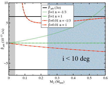
Figure 7: Orbital period derivative versus companion star mass in the hypothesis of conservative and non-conservative mass transfer (with mass leaving the system with the specific angular momentum at the inner Lagrangian point). Dotted and dashed-dotted green curves represent the conservative ($\beta=1$) mass-transfer scenario assuming a low-main sequence ($n=1$) and a fully convective ($n=-1/3$) companion star, respectively. Dashed and dot-dot-dashed red curves represent the non-conservative ($\beta=t_{out}/t_{quiet}\simeq 0.01$) mass-transfer scenario again for a low-main sequence ($n=1$) and a fully convective ($n=-1/3$) companion star, respectively. The horizontal black lines delimit the $3\sigma$ orbital period derivative confidence level interval obtained from the analysis. Finally, vertical lines represent the minimum mass estimated from the binary mass function (for a 1.4 M_⊙ NS) and the companion mass for an almost face-on system (i=$10^{\circ}$).

We investigated the NS spin frequency secular evolution by comparing the spin frequency at the end of the second outburst observed in 2008 with the value at the beginning of the latest outburst. Following Papitto et al. (2011), the 2008 mean spin frequency was $\nu=598.89213082(2)$ Hz, with an upper limit on the spin-up derivative of $|\dot{\nu}|<4.5\times 10^{-13}$ Hz/s , estimated for an outburst duration of $\sim 10$ days. Combining these information we estimated a frequency value $\nu_{2008}=598.8921308(4)$ Hz at the end of the outburst. Under the assumption that the spin value obtained from the XMM-Newton observation (see Tab. 2) is a good proxy of the NS spin of the beginning of the 2015 outburst we found $\Delta\nu=\nu_{2015}-\nu_{2008}=(1\pm 4)\times 10^{-7}$ Hz, corresponding to a $3\sigma$ confidence level interval $-11\times 10^{-7}$ Hz $<\Delta\nu<13\times 10^{-7}$ Hz. For a quiescence period between the two most recent outbursts of $\Delta t=2491$ days we estimated a $3\sigma$ confidence level interval for the spin frequency derivative during quiescence $-5\times 10^{-15}$ Hz/s $<\dot{\nu}<6\times 10^{-15}$ Hz/s, still consistent with the spin-down derivative $\dot{\nu}_{sd}\sim-4\times 10^{-16}$ Hz measured between the first two outbursts of the source (see e.g. Papitto et al., 2011; Patruno, 2010; Hartman et al., 2011).

Another interesting aspect of IGR J00291$+$5934 is the complex behaviour of its pulse profile as function of energy. As shown in the top panel of Fig 4, the time lags resemble a piecewise function with two energy intervals where the lags increase as a function of energy (with an increment of $\sim 20\mu$s in the interval $0.3-1.6$ keV and an increment of $\sim 80\mu$s between $7-80$ keV), separated by the region $1.6-7$ keV where a clear decrement ($\sim 170\mu$s) of the lags is observed. This result is consistent with Falanga et al. (2005), who investigated the energy dependence of the pulse profile of IGR J00291$+$5934 combining the observations collected by RXTE and INTEGRAL. A very similar behaviour has been observed in the AMXP IGR J17511$-$3057 (Riggio et al., 2011; Falanga et al., 2011). In analogy with the lags, a complex behaviour is shown by the pulse fractional amplitude (Fig. 4, bottom panel) that increases from 6% at 0.5 keV up to 17% at 3 keV and then decreases down to 9% at 10 keV. This behaviour is peculiar for the source, as generally AMXPs show also well pulsating hard components (e.g. Gierliński & Poutanen, 2005). Above 10 keV, the fractional amplitude seems to increase again, even though the large uncertainties make the trend less prominent. We note that our estimates of the fractional amplitude are compatible with Falanga et al. (2005) above 10 keV. On the other hand, between 2 and 10 keV, both the amplitude and trend as a function of energy are clearly different (see their Fig. 8). This discrepancy likely reflects the large background contamination of RXTE due to the one degree spatial resolution. The origin of the pulse profile dependence with energy is still unclear; however, mechanisms such as strong Comptonization of the beamed radiation have been proposed to explain the hard spectrum of the pulsation, as well as the lags observed in few AMXPs (e.g. Patruno et al., 2009; Papitto et al., 2010) including IGR J00291$+$5934 (Falanga & Titarchuk, 2007).

References

- Alpar et al. (1982) Alpar M. A., Cheng A. F., Ruderman M. A., Shaham J., 1982, Nature, 300, 728
- Altamirano et al. (2011) Altamirano D., Belloni T., Linares M., van der Klis M., Wijnands R., Curran P. A., Kalamkar M., Stiele H., Motta S., Muñoz-Darias T., Casella P., Krimm H., 2011, ApJ, 742, L17
- Anders & Grevesse (1989) Anders E., Grevesse N., 1989, Geochim. Cosmochim. Acta, 53, 197
- Applegate (1992) Applegate J. H., 1992, ApJ, 385, 621
- Applegate & Shaham (1994) Applegate J. H., Shaham J., 1994, ApJ, 436, 312
- Archibald et al. (2015) Archibald A. M., Bogdanov S., Patruno A., Hessels J. W. T., Deller A. T., Bassa C., Janssen G. H., Kaspi V. M., Lyne A. G., Stappers B. W., Tendulkar S. P., D’Angelo C. R., Wijnands R., 2015, ApJ, 807, 62
- Arzoumanian et al. (1994) Arzoumanian Z., Fruchter A. S., Taylor J. H., 1994, ApJ, 426, 85
- Bassa et al. (2014) Bassa C. G., Patruno A., Hessels J. W. T., Keane E. F., Monard B., Mahony E. K., Bogdanov S., Corbel S., Edwards P. G., Archibald A. M., Janssen G. H., Stappers B. W., Tendulkar S., 2014, MNRAS, 441, 1825
- Bevington & Robinson (2003) Bevington P. R., Robinson D. K., 2003, Data reduction and error analysis for the physical sciences
- Bozzo et al. (2015) Bozzo E., Papitto A., Sanna A., Falanga M., Campana S., Salvo T. d., Iaria R., Pintore F., Riggio A., Egron E., 2015, The Astronomer’s Telegram, 7852
- Burderi et al. (2002) Burderi L., D’Antona F., Burgay M., 2002, ApJ, 574, 325
- Burderi & Di Salvo (2013) Burderi L., Di Salvo T., 2013, Mem. Soc. Astron. Italiana, 84, 117
- Burderi et al. (2007) Burderi L., Di Salvo T., Lavagetto G., Menna M. T., Papitto A., Riggio A., Iaria R., D’Antona F., Robba N. R., Stella L., 2007, ApJ, 657, 961
- Burderi et al. (2001) Burderi L., Possenti A., D’Antona F., Di Salvo T., Burgay M., Stella L., Menna M. T., Iaria R., Campana S., d’Amico N., 2001, ApJ, 560, L71
- Burderi et al. (2009) Burderi L., Riggio A., di Salvo T., Papitto A., Menna M. T., D’Aì A., Iaria R., 2009, A&A, 496, L17
- D’Aì et al. (2010) D’Aì A., di Salvo T., Ballantyne D., Iaria R., Robba N. R., Papitto A., Riggio A., Burderi L., Piraino S., Santangelo A., Matt G., Dovčiak M., Karas V., 2010, A&A, 516, A36
- De Falco et al. (2016) De Falco V., Kuiper L., Bozzo E., Galloway D. K., Poutanen J., Ferrigno C., Stella L., Falanga M., 2016, ArXiv e-prints
- Degenaar et al. (2016) Degenaar N., Pinto C., Miller J. M., Wijnands R., Altamirano D., Paerels F., Fabian A. C., Chakrabarty D., 2016, MNRAS
- Di Salvo et al. (2008) Di Salvo T., Burderi L., Riggio A., Papitto A., Menna M. T., 2008, MNRAS, 389, 1851
- Di Salvo et al. (2015) Di Salvo T., Iaria R., Matranga M., Burderi L., D’Aí A., Egron E., Papitto A., Riggio A., Robba N. R., Ueda Y., 2015, MNRAS, 449, 2794
- Doroshenko et al. (2001) Doroshenko O., Löhmer O., Kramer M., Jessner A., Wielebinski R., Lyne A. G., Lange C., 2001, A&A, 379, 579
- Eckert et al. (2004) Eckert D., Walter R., Kretschmar P., Mas-Hesse M., Palumbo G. G. C., Roques J.-P., Ubertini P., Winkler C., 2004, The Astronomer’s Telegram, 352
- Fabian et al. (1989) Fabian A. C., Rees M. J., Stella L., White N. E., 1989, MNRAS, 238, 729
- Falanga et al. (2005) Falanga M., Kuiper L., Poutanen J., Bonning E. W., Hermsen W., di Salvo T., Goldoni P., Goldwurm A., Shaw S. E., Stella L., 2005, A&A, 444, 15
- Falanga et al. (2011) Falanga M., Kuiper L., Poutanen J., Galloway D. K., Bonning E. W., Bozzo E., Goldwurm A., Hermsen W., Stella L., 2011, A&A, 529, A68
- Falanga & Titarchuk (2007) Falanga M., Titarchuk L., 2007, ApJ, 661, 1084
- Ferrigno et al. (2016) Ferrigno C., Bozzo E., Sanna A., Pintore F., Papitto A., Riggio A., Burderi L., Di Salvo T., Iaria R., D’Aì A., 2016, ArXiv e-prints
- Frank et al. (1987) Frank J., King A. R., Lasota J.-P., 1987, A&A, 178, 137
- Galloway et al. (2005) Galloway D. K., Markwardt C. B., Morgan E. H., Chakrabarty D., Strohmayer T. E., 2005, ApJ, 622, L45
- Gierliński & Poutanen (2005) Gierliński M., Poutanen J., 2005, MNRAS, 359, 1261
- Hartman et al. (2011) Hartman J. M., Galloway D. K., Chakrabarty D., 2011, ApJ, 726, 26
- Hartman et al. (2008) Hartman J. M., Patruno A., Chakrabarty D., Kaplan D. L., Markwardt C. B., Morgan E. H., Ray P. S., van der Klis M., Wijnands R., 2008, ApJ, 675, 1468
- Hartman et al. (2009) Hartman J. M., Patruno A., Chakrabarty D., Markwardt C. B., Morgan E. H., van der Klis M., Wijnands R., 2009, ApJ, 702, 1673
- in ’t Zand et al. (1999) in ’t Zand J. J. M., Verbunt F., Strohmayer T. E., Bazzano A., Cocchi M., Heise J., van Kerkwijk M. H., Muller J. M., Natalucci L., Smith M. J. S., Ubertini P., 1999, A&A, 345, 100
- Kolehmainen et al. (2011) Kolehmainen M., Done C., Diaz Trigo M., 2011, ArXiv e-prints
- Laurent & Titarchuk (2007) Laurent P., Titarchuk L., 2007, ApJ, 656, 1056
- Linares et al. (2007) Linares M., van der Klis M., Wijnands R., 2007, ApJ, 660, 595
- Lyne & Graham-Smith (1990) Lyne A. G., Graham-Smith F., 1990, Pulsar astronomy. Cambridge University Press
- Madsen et al. (2015) Madsen K. K., Harrison F. A., Markwardt C. B., An H., Grefenstette B. W., Bachetti M., Miyasaka H., Kitaguchi T., Bhalerao V., Boggs S., Christensen F. E., Craig W. W., Forster K., Fuerst F., 2015, ApJS, 220, 8
- Neilsen et al. (2012) Neilsen J., Remillard R. A., Lee J. C., 2012, ApJ, 750, 71
- Paizis et al. (2005) Paizis A., Nowak M. A., Wilms J., Courvoisier T. J.-L., Ebisawa K., Rodriguez J., Ubertini P., 2005, A&A, 444, 357
- Papitto et al. (2015) Papitto A., de Martino D., Belloni T. M., Burgay M., Pellizzoni A., Possenti A., Torres D. F., 2015, MNRAS, 449, L26
- Papitto et al. (2009) Papitto A., Di Salvo T., D’Aì A., Iaria R., Burderi L., Riggio A., Menna M. T., Robba N. R., 2009, A&A, 493, L39
- Papitto et al. (2013) Papitto A., Ferrigno C., Bozzo E., Rea N., Pavan L., Burderi L., Burgay M., Campana S., di Salvo T., Falanga M., Filipović M. D., Freire P. C. C., Hessels J. W. T., Possenti A., Ransom S. M., Riggio A., 2013, Nature, 501, 517
- Papitto et al. (2011) Papitto A., Riggio A., Burderi L., di Salvo T., D’Aí A., Iaria R., 2011, A&A, 528, A55
- Papitto et al. (2010) Papitto A., Riggio A., di Salvo T., Burderi L., D’Aì A., Iaria R., Bozzo E., Menna M. T., 2010, MNRAS, 407, 2575
- Patruno (2010) Patruno A., 2010, ApJ, 722, 909
- Patruno (2016) Patruno A., 2016, ArXiv e-prints
- Patruno et al. (2010) Patruno A., Altamirano D., Watts A., Armas Padilla M., Cavecchi Y., Degenaar N., Kalamkar M., Kaur R., Soleri P., Yang Y. J., van der Klis M., Wijnands R., Casella P., Linares M., Rea N., Heinke C. O., Pooley D., 2010, The Astronomer’s Telegram, 2407, 1
- Patruno et al. (2012) Patruno A., Bult P., Gopakumar A., Hartman J. M., Wijnands R., van der Klis M., Chakrabarty D., 2012, ApJ, 746, L27
- Patruno et al. (2009) Patruno A., Rea N., Altamirano D., Linares M., Wijnands R., van der Klis M., 2009, MNRAS, 396, L51
- Patruno & Watts (2012) Patruno A., Watts A. L., 2012, ArXiv e-prints
- Pintore et al. (2014) Pintore F., Sanna A., Di Salvo T., Guainazzi M., D’Aì A., Riggio A., Burderi L., Iaria R., Robba N. R., 2014, MNRAS, 445, 3745
- Poutanen et al. (2007) Poutanen J., Lipunova G., Fabrika S., Butkevich A. G., Abolmasov P., 2007, MNRAS, 377, 1187
- Riggio et al. (2007) Riggio A., di Salvo T., Burderi L., Iaria R., Papitto A., Menna M. T., Lavagetto G., 2007, MNRAS, 382, 1751
- Riggio et al. (2011) Riggio A., Papitto A., Burderi L., di Salvo T., Bachetti M., Iaria R., D’Aì A., Menna M. T., 2011, A&A, 526, A95
- Sanna et al. (2016) Sanna A., Burderi L., Riggio A., Pintore F., Di Salvo T., Gambino A. F., Iaria R., Matranga M., Scarano F., 2016, MNRAS, 459, 1340
- Sanna et al. (2015) Sanna A., Pintore F., Riggio A., Burderi L., Di Salvo T., Iaria R., Scarano F., Papitto A., Bozzo E., 2015, The Astronomer’s Telegram, 7836
- Stappers et al. (2014) Stappers B. W., Archibald A. M., Hessels J. W. T., Bassa C. G., Bogdanov S., Janssen G. H., Kaspi V. M., Lyne A. G., Patruno A., Tendulkar S., Hill A. B., Glanzman T., 2014, ApJ, 790, 39
- Torres et al. (2008) Torres M. A. P., Jonker P. G., Steeghs D., Roelofs G. H. A., Bloom J. S., Casares J., Falco E. E., Garcia M. R., Marsh T. R., Mendez M., Miller J. M., Nelemans G., Rodríguez-Gil P., 2008, ApJ, 672, 1079