On a consistent estimator of a useful signal in Ornstein-Uhlenbeck stochastic model in $\mathbb{C}[-l,l[$

Abstract.

It is considered a transmittion process of a useful signal in Ornstein-Uhlenbeck stochastic model in $\mathbb{C}[-l,l[$ defined by the stochastic differential equation

$$d\Psi(t,x,\omega)=\sum_{n=0}^{2m}A_{n}\frac{\partial^{n}}{\partial x^{n}}\Psi(t,x,\omega)dt+\sigma dW(t,\omega)$$

with initial condition

$$\Psi(0,x,\omega)=\Psi_{0}(x)\in FD^{(0)}[-l,l[,$$

where $m\geq 1$, $(A_{n})_{0\leq n\leq 2m}\in\mathbb{R}^{+}\times\mathbb{R}^{2m-1}$,$~{}((t,x,\omega)\in[0,+\infty[\times[-l,l[\times\Omega)$, $\sigma\in\mathbb{R}^{+}$, $\mathbb{C}[-l,l[$ is Banach space of all real-valued bounded continuous functions on $[-l,l[$, $FD^{(0)}[-l,l[\subset\mathbb{C}[-l,l[$ is class of all real-valued bounded continuous functions on $[-l,l[$ whose Fourier series converges to himself everywhere on $[-l,l[$, $(W(t,\omega))_{t\geq 0}$ is a Wiener process and $\Psi_{0}(x)$ is a useful signal.

By use a sequence of transformed signals $(Z_{k})_{k\in N}=(\Psi(t_{0},x,\omega_{k}))_{k\in N}$ at moment $t_{0}>0$, consistent and infinite-sample consistent estimates of the useful signal $\Psi_{0}$ is constructed under assumption that parameters $(A_{n})_{0\leq n\leq 2m}$ and $\sigma$ are known. Animation and simulation of the Ornstein-Uhlenbeck process in Banach space $\mathbb{C}[-l,l[$ and results of calculations of estimates of a useful signal in the same stochastic model are also presented.

.

1. Introduction

Suppose that $\Theta$ is a vector subspace of the Banach space $\mathbb{C}[-l,l[$ equipped with usual norm, where $\mathbb{C}[-l,l[$ denotes the class of all bounded continuous functions on $[-l,l[$.

In the information transmitting theory we consider Ornstein-Uhlenbeck stochastic system

$$\xi(t,x,\omega)_{x\in[-l,l[}=e^{t\sum_{n=0}^{2m}A_{n}\frac{\partial^{n}}{\partial x^{n}}}\theta(x)_{x\in[-l,l[}+$$

$(1.1)$ $$\sigma\int_{0}^{t}e^{(t-\tau)\sum_{n=0}^{2m}A_{n}\frac{\partial^{n}}{\partial x^{n}}}\times I_{[-l,l[}(x)dW(\tau,\omega),$$

where $(A_{n})_{0\leq n\leq 2m}\in\mathbb{R}^{+}\times\mathbb{R}^{2m-1}(m\geq 1)$, $\theta\in\Theta$ is a useful signal, $(W(t,\cdot))_{t\geq 0}$ is Winner processes(the so-called “white noises” ) defined on the probability space $(\Omega,{{\bf F}},P)$, $(\xi(t,\cdot,\omega))$(equivalently, $\xi(t,x,\omega)_{x\in[-l,l[}$) is a transformed signal for $(t,\omega)\in[0,+\infty[\times\Omega)$, $I_{[-l,l[}$ denotes the indicator function of the interval $[-l,l[$.

Let $\mu$ be a Borel probability measure on $\mathbb{C}^{[0,+\infty[}[-l,l[$ defined by generalized “white noise”

$(1.2)$ $$\big{(}\sigma\int_{0}^{t}e^{(t-\tau)\sum_{n=0}^{2m}A_{n}\frac{\partial^{n}}{\partial x^{n}}}\times I_{[-l,l[}dW(\tau,\omega)\big{)}_{t\geq 0}.$$

Then we have

$$(\forall X)(X\in{\bf B}\big{(}\mathbb{C}^{[0,+\infty[}[-l,l[\big{)}\rightarrow\mu(X)=P(\{\omega:\omega\in\Omega~{}$$

$(1.3)$ $$\&~{}\big{(}\sigma\int_{0}^{t}e^{(t-\tau)\sum_{n=0}^{2m}A_{n}\frac{\partial^{n}}{\partial x^{n}}}\times I_{[-l,l[}dW_{k}(\tau,\omega)\big{)}_{t\geq 0}\in X\})),$$

where ${\bf B}\big{(}\mathbb{C}^{[0,+\infty[}[-l,l[\big{)}$ is the Borel $\sigma$-algebra of subsets of the space $\mathbb{C}^{[0,+\infty[}[-l,l[$.

Let $\lambda$ be a Borel probability measure on $\mathbb{C}^{[0,+\infty[}[-l,l[$ defined by transformed signal $\xi(t,x,\omega)$ that is

$$(\forall X)(X\in{\bf B}\big{(}\mathbb{C}^{[0,+\infty[}[-l,l[\big{)}\rightarrow\mu(X)=P(\{\omega:\omega\in\Omega~{}$$

$(1.4)$ $$\&~{}\big{(}\xi(t,x,\omega)\big{)}_{t\geq 0}\in X\})),$$

In the information transmitting theory, the general decision is that the Borel probability measure $\lambda$, defined by the transformed signal coincide with $e^{t\sum_{n=0}^{2m}A_{n}\frac{\partial^{n}}{\partial x^{n}}}\theta$ shift $\mu_{\theta}$ of the measure $\mu$ for some $\theta_{0}\in\Theta$ provided that

$(1.5)$ $$(\exists\theta_{0})(\theta_{0}\in\Theta\rightarrow(\forall X)(X\in{\bf B}\big{(}\mathbb{C}^{[0,+\infty[}[-l,l[\big{)}\rightarrow\lambda(X)=\mu_{\theta}(X)),$$

where $\mu_{\theta}(\cdot)=\mu(\cdot+\big{(}e^{t\sum_{n=0}^{2m}A_{n}\frac{\partial^{n}}{\partial x^{n}}}\theta\big{)}_{t\geq 0})$.

Here we consider a particular case of the above model when a vector space of useful signals $\Theta$ coincides with $FD^{0}[-l,l[$, where $FD^{0}[-l,l[\subset\mathbb{C}[-l,l[$ denotes a vector space of all bounded continuous real-valued functions on $[-l,l[$ whose Fourier series converges to himself everywhere on $[-l,l[$.

Definition 1.1.

Following [11], a triplet

$(1.6)$ $$(\big{(}\mathbb{C}^{[0,+\infty[}[-l,l[\big{)}^{\mathbb{N}},{\bf B}\big{(}\big{(}\mathbb{C}^{[0,+\infty[}[-l,l[\big{)}^{\mathbb{N}}\big{)},\mu^{\mathbb{N}}_{\theta}\big{)}_{\theta\in\Theta}$$

is called a statistical structure described the stochastic system (1.1).

Definition 1.2.

Following [11], a Borel measurable function $T_{n}:\big{(}\mathbb{C}^{[0,+\infty[}[-l,l[\big{)}^{n}\to\Theta~{}(n\in\mathbb{N})$ is called a consistent estimate of a parameter $\theta$ for the family $(\mu_{\theta}^{\mathbb{N}})_{\theta\in\Theta}$ if the condition

$(1.7)$ $$\mu_{\theta}^{\mathbb{N}}(\{(x_{k})_{k\in\mathbb{N}}:~{}(x_{k})_{k\in\mathbb{N}}\in\big{(}\mathbb{C}^{[0,+\infty[}[-l,l[\big{)}^{\mathbb{N}}~{}\&~{}\lim_{n\to\infty}||T_{n}(x_{1},\cdots,x_{n})-\theta||=0\})=1$$

holds for each $\theta\in\Theta$, where $||\cdot||$ is a usual norm in $\mathbb{C}[-l,l[$.

Definition 1.3.

Following [11], a Borel measurable function $T:\big{(}\mathbb{C}^{[0,+\infty[}[-l,l[\big{)}^{\mathbb{N}}\to\Theta$ is called an infinite-sample consistent estimate of a parameter $\theta$ for the family $(\mu_{\theta}^{\mathbb{N}})_{\theta\in\Theta}$ if the condition

$(1.8)$ $$\mu_{\theta}^{\mathbb{N}}(\{(x_{k})_{k\in\mathbb{N}}:~{}(x_{k})_{k\in\mathbb{N}}\in\big{(}\mathbb{C}^{[0,+\infty[}[-l,l[\big{)}^{\mathbb{N}}~{}\&~{}T((x_{k})_{k\in\mathbb{N}})=\theta\})=1$$

holds for each $\theta\in\Theta$.

The main goal of the present paper is construct consistent and infinite-sample estimators of the useful signal for the stochastic model (1.1) which is a particular case of the Ornstein-Uhlenbeck process in $\mathbb{C}[-l,l[$. Concerning estimations of parameters for another versions of the Ornstein-Uhlenbeck processes the reader can consult with [2], [7],[5], [4].

The rest of the present paper is the following.

Section 2 contains some auxiliary notions and fact from theories of ordinary and stochastic differential equations.

In Section 3 we present our main results.

In Section 4 we present animations and simulations of the Ornstein-Uhlenbeck process in $\mathbb{C}[-l,l[$ and present results of calculations of the estimator of a useful signal when parameters $(A_{n})_{0\leq n\leq 2m}$,$\sigma$ and a sample of transformed signals at moment $t_{0}>0$ defined by $(1.1)$ are known.

In Section 5 we consider discussion and conclusion.

2. Materials and methods

We begin this section by a short description of a certain result concerning a solution of some differential equations with initial value problem obtained in the paper [6]. Further, by use this approach and technique developed in [8], their some applications for a solution of the Ornstein-Uhlenbeck stochastic differential equation in $\mathbb{C}[-l,l[$ are obtained. At end of this section, well known Kolmogorov Strong Law of Large Numbers is presented.

Lemma 2.1 ([6], Corollary 2.1, p. 6).

For $m\geq 1$, let us consider a linear partial differential equation

$(2.1)$ $$\frac{\partial}{\partial t}\Psi(t,x)=\sum_{n=0}^{2m}A_{n}\frac{\partial^{n}}{\partial x^{n}}\Psi(t,x)~{}((t,x)\in[0,+\infty[\times[-l,l[)$$

with initial condition

$(2.2)$ $$\Psi(0,x)=\frac{c_{0}}{2}+\sum_{k=1}^{\infty}c_{k}\cos\Big{(}\frac{k\pi x}{l}\Big{)}+d_{k}\sin\Big{(}\frac{k\pi x}{l}\Big{)}\in FD^{(0)}[-l,l[.$$

If $(\frac{c_{0}}{2},c_{1},d_{1},c_{2},d_{2},\dots)$ is such a sequence of real numbers that a series $\Psi(t,x)$ defined by

$$\Psi(t,x)=\frac{e^{tA_{0}}c_{0}}{2}+\sum_{k=1}^{\infty}e^{\sigma_{k}t}\Big{(}(c_{k}\cos(\omega_{k}t)+$$

$(2.3)$ $$d_{k}\sin(\omega_{k}t))\cos(\frac{k\pi x}{l})+(d_{k}\cos(\omega_{k}t)-c_{k}\sin(\omega_{k}t))\sin(\frac{k\pi x}{l})\Big{)}$$

belongs to the class $FD^{(2m)}[-l,l[$ as a series of a variable $x$ for all $t\geq 0$, and is differentiable term by term as a series of a variable $t$ for all $x\in[-l,l[$, then $\Psi$ is a solution of $(2.1)$-$(2.2)$.

By use an approach developed in [8], we get the validity of the following assertion.

Lemma 2.2.

For $m\geq 1$, let us consider Ornstein-Uhlenbeck process in $\mathbb{C}[-l,l[$ defined by the stochastic differential equation

$(2.4)$ $$d\Psi(t,x,\omega)=\sum_{n=0}^{2m}A_{n}\frac{\partial^{n}}{\partial x^{n}}\Psi(t,x,\omega)dt+\sigma dW(t,\omega)I_{[-l,l[}(x)~{}((t,x,\omega)\in[0,+\infty[\times[-l,l[\times\Omega)$$

with initial condition

$(2.5)$ $$\Psi(0,x,\omega)=\Psi_{0}(x),$$

where $(A_{n})_{0\leq n\leq 2m}\in\mathbb{R}^{+}\times\mathbb{R}^{2m-1}$,$(W(t,\omega))_{t\geq 0}$ is a Wiener process and

$(2.6)$ $$\Psi_{0}(x)=\frac{c_{0}}{2}+\sum_{k=1}^{\infty}c_{k}\cos\Big{(}\frac{k\pi x}{l}\Big{)}+d_{k}\sin\Big{(}\frac{k\pi x}{l}\Big{)}\in FD^{(0)}[-l,l[.$$

If $(\frac{c_{0}}{2},c_{1},d_{1},c_{2},d_{2},\dots)$ is such a sequence of real numbers that a series

$$\frac{e^{tA_{0}}c_{0}}{2}+\sum_{k=1}^{\infty}e^{\sigma_{k}t}\Big{(}(c_{k}\cos(\omega_{k}t)+$$

$(2.7)$ $$d_{k}\sin(\omega_{k}t))\cos(\frac{k\pi x}{l})+(d_{k}\cos(\omega_{k}t)-c_{k}\sin(\omega_{k}t))\sin(\frac{k\pi x}{l})\Big{)}+\sigma\int_{0}^{t}e^{(t-\tau)A_{0}}dW_{\tau}(\omega)I_{[-l,l[}(x)$$

belongs to the class $FD^{(2m)}[-l,l[$ as a series of a variable $x$ for all $t\geq 0,\omega\in\Omega$, and is differentiable term by term as a series of a variable $t$ for all $x\in[-l,l[,\omega\in\Omega$, then the solution of $(2.5)$-$(2.6)$ is given by

$$\Psi(t,x,\omega)=e^{t\sum_{n=0}^{2m}A_{n}\frac{\partial^{n}}{\partial x^{n}}}(\Psi(0,x,\omega))+\sigma\int_{0}^{t}e^{(t-s)\sum_{n=0}^{2m}A_{n}\frac{\partial^{n}}{\partial x^{n}}}dW(s,\omega).$$

Proof.

Putting $\mathbb{A}=\sum_{n=0}^{2m}A_{n}\partial^{n}/\partial x^{n}$ and $f(t,\Psi(t,x,\omega))=e^{-t\mathbb{A}}\Psi(t,x,\omega),$ we get

$$df(t,\Psi(t,x,\omega))=-\mathbb{A}e^{-t\mathbb{A}}\Psi(t,x,\omega)dt+e^{-t\mathbb{A}}d\Psi(t,x,\omega)$$

$$=-\mathbb{A}e^{-t\mathbb{A}}\Psi(t,x,\omega)dt+e^{-t\mathbb{A}}(\mathbb{A}\Psi(t,x,\omega)+\sigma dW(t,\omega))=\sigma e^{-t\mathbb{A}}dW(t,\omega).$$

By integration of both sides we get

$$f(t,\Psi(t,x,\omega))-f(0,\Psi(0,x,\omega))=\sigma\int_{0}^{t}e^{-\tau\mathbb{A}}dW(\tau,\omega)$$

which implies

$$e^{-t\mathbb{A}}\Psi(t,x,\omega)-e^{-0\mathbb{A}}\Psi(0,x,\omega)=\sigma\int_{0}^{t}e^{-\tau\mathbb{A}}dW(\tau,\omega).$$

Now we get

$$e^{t\mathbb{A}}(e^{-t\mathbb{A}}(\Psi(t,x,\omega))-e^{t\mathbb{A}}(e^{-0\mathbb{A}}(\Psi(0,x,\omega)))=e^{t\mathbb{A}}(\sigma\int_{0}^{t}e^{-\tau\mathbb{A}}dW(\tau,\omega)),$$

which is equivalent to the equality

$$\Psi(t,x,\omega))=e^{t\mathbb{A}}(\Psi(0,x,\omega))+\sigma\int_{0}^{t}e^{(t-\tau)\mathbb{A}}I_{[-l,l[}(x)dW(\tau,\omega)).$$

∎

Remark 2.3.

Under condition of Lemma 2.2 we have

$$\Psi(t,x,\omega)=\frac{e^{tA_{0}}c_{0}}{2}+\sum_{k=1}^{\infty}e^{\sigma_{k}t}\Big{(}(c_{k}\cos(\omega_{k}t)+$$

$$d_{k}\sin(\omega_{k}t))\cos(\frac{k\pi x}{l})+(d_{k}\cos(\omega_{k}t)-c_{k}\sin(\omega_{k}t))\sin(\frac{k\pi x}{l})\Big{)}+$$

$(2.8)$ $$\sigma\int_{0}^{t}e^{(t-\tau)A_{0}}I_{[-l,l[}(x)dW(\tau,\omega)).$$

Lemma 2.4.

Under conditions of Lemma 2.2, the following conditions are valid:

(i)  $E\Psi(t,x,\cdot)=\frac{e^{tA_{0}}c_{0}}{2}+\sum_{k=1}^{\infty}e^{\sigma_{k}t}\Big{(}(c_{k}\cos(\omega_{k}t)+d_{k}\sin(\omega_{k}t))\cos(\frac{k\pi x}{l})$

$+(d_{k}\cos(\omega_{k}t)-c_{k}\sin(\omega_{k}t))\sin(\frac{k\pi x}{l})\Big{)};$

(ii)   $\mbox{cov}(\Psi(s,x,\cdot),\Psi(t,x,\cdot))=\frac{\sigma^{2}}{2A_{0}}\left(e^{-A_{0}(t-s)}-e^{-A_{0}(t+s)}\right);$

(iii)  $\mbox{var}(\Psi(s,x,\cdot))=\frac{\sigma^{2}}{2A_{0}}\left(1-e^{-2A_{0}s}\right);$

Proof.

The validity of the item (i) is obvious. In order to prove the validity of the items (ii)-(iii), we can use the Ito isometry to calculate the covariance function by

$$\mbox{cov}(\Psi(s,x,\cdot),\Psi(t,x,\cdot))=E[(\Psi(s,x,\cdot)-E[\Psi(s,x,\cdot)])(\Psi(s,t,\cdot)-E[\Psi(s,t,\cdot)])]$$

$$=E\left[\int_{0}^{s}\sigma e^{A_{0}(u-s)}\,dW(u,\omega)\int_{0}^{t}\sigma e^{A_{0}(v-t)}\,dW(v,\omega)\right]$$

$$=\sigma^{2}e^{-A_{0}(s+t)}E\left[\int_{0}^{s}e^{A_{0}u}\,dW(u,\omega)\int_{0}^{t}e^{A_{0}v}\,dW(v,\omega)\right]$$

$$=\frac{\sigma^{2}}{2A_{0}}\,e^{-A_{0}(s+t)}(e^{2A_{0}\min(s,t)}-1).$$

Thus if $s<t$(so that $min(s,t)=s$), then we have

$$\mbox{cov}(\Psi(s,x,\cdot),\Psi(t,x,\cdot))=\frac{\sigma^{2}}{2A_{0}}\left(e^{-A_{0}(t-s)}-e^{-A_{0}(t+s)}\right).$$

Similarly, if $s=t$ (so that $min(s,t)=s)$, then we have

$$\mbox{var}(\Psi(s,x,\cdot))=\frac{\sigma^{2}}{2A_{0}}\left(1-e^{-2A_{0}s}\right).$$

∎

In the next section we will need the well known fact from the probability theory (see, for example, [9], p. 390).

Lemma 2.5.

(Kolmogorov’s strong law of large numbers) Let $X_{1},X_{2},...$ be a sequence of independent identically distributed random variables defined on the probability space $(\Omega,\mathcal{F},P)$. If these random variables have a finite expectation $m$ (i.e., $E(X_{1})=E(X_{2})=...=m<\infty$), then the following condition

$(2.9)$ $$P(\{\omega:\lim_{n\to\infty}n^{-1}\sum_{k=1}^{n}X_{k}(\omega)=m\})=1$$

holds true.

3. Results

In this section, by the use of Kolmogorov Strong Law of Large Numbers we construct a consistent and an infinite-sample consistent estimators of a useful signal which is transmitted by the Ornstein-Uhlenbeck stochastic system (1.1).

Theorem 3.1.

Let consider $\mathbb{C}[-l,l[$-valued stochastic process $(\xi(t,x,\omega)_{x\in[-l,l[})_{t\geq 0}$ defined by

$(3.1)$ $$\xi(t,x,\omega)_{x\in[-l,l[}=e^{t\mathbb{A}}(\theta(x)_{x\in[-l,l[})+\sigma\int_{0}^{t}e^{(t-\tau)\mathbb{A}}I_{[-l,l[}(x)_{x\in[-l,l[}dW(\tau,\omega),$$

where $\theta\in FD^{(0)}$ and $\mathbb{A}=\sum_{n=0}^{2m}A_{n}\frac{\partial^{n}}{\partial x^{n}}$. Assume that all conditions of Lemma 2.9 are satisfied. For a fixed $t=t_{0}>0$, we denote by $\mu_{\theta}$ a probability measure in $\mathbb{C}[-l,l[$ defined by the random element $(\Xi(t_{0},\omega))$. For each $(Z_{k})_{k\in\mathbb{N}}\in\big{(}\mathbb{C}[-l,l[\big{)}^{\mathbb{N}}$ we put

$(3.2)$ $$T_{n}((Z_{k})_{k\in\mathbb{N}})=e^{-t_{0}\mathbb{A}}(\frac{\sum_{k=1}^{n}Z_{k}}{n}).$$

Then $T_{n}$ is a consistent estimate of a useful signal $\theta$ provided that

$(3.3)$ $$\mu_{\theta}^{\mathbb{N}}\{(Z_{k})_{k\in\mathbb{N}}:\lim_{n\to\infty}||T_{n}((Z_{k})_{k\in\mathbb{N}})-\theta||=0\}=1$$

for each $\theta\in FD^{(0)}[-l,l[.$

Proof.

For each $X\in B\big{(}\mathbb{C}[-l,l[\big{)}$ we have

$$\mu_{\theta}(X)=P\{\omega:\Xi(t_{0},\omega)\in X\}=P\{\omega:e^{t_{0}\mathbb{A}}(\theta)+\sigma\int_{0}^{t_{0}}e^{(t_{0}-\tau)\mathbb{A}}I_{[-l,l[}dW(\tau,\omega))\in X\}=$$

$$P\{\omega:\sigma\int_{0}^{t_{0}}e^{(t_{0}-\tau)A_{0}}dW(\tau,\omega))I_{[-l,l[}\in\big{(}X-e^{t_{0}\mathbb{A}}(\theta)\big{)}\cap\{\alpha I_{[-l,l[}:\alpha\in\mathbb{R}\}\}.$$

We have

$$\mu_{\theta}^{\mathbb{N}}\{(Z_{k})_{k\in\mathbb{N}}:\lim_{n\to\infty}||T_{n}((Z_{k})_{k\in\mathbb{N}})-\theta||=0\}=$$

$$\mu_{\theta}^{\mathbb{N}}\{(Z_{k})_{k\in\mathbb{N}}:\lim_{n\to\infty}||e^{-t_{0}\mathbb{A}}(\frac{\sum_{k=1}^{n}Z_{k}}{n})-\theta||=0\}=$$

$$\mu_{\theta}^{\mathbb{N}}\{(Z_{k})_{k\in\mathbb{N}}:\lim_{n\to\infty}||\frac{\sum_{k=1}^{n}Z_{k}}{n}-e^{t_{0}\mathbb{A}}(\theta)||=0\}=$$

$$\mu_{\theta}^{\mathbb{N}}\{(Z_{k})_{k\in\mathbb{N}}:Z_{k}\in\{\alpha_{k}I_{[-l,l[}:\alpha_{k}\in\mathbb{R}\}+e^{t_{0}\mathbb{A}}(\theta)~{}\&~{}\lim_{n\to\infty}||\frac{\sum_{k=1}^{n}Z_{k}}{n}-e^{t\mathbb{A}}(\theta)||=0\}=$$

$$\mu_{\theta}^{\mathbb{N}}\{(Z_{k})_{k\in\mathbb{N}}:(\exists(\beta_{k})_{k\in N}\in\mathbb{R}^{\infty})(Z_{k}=\beta_{k}I_{[-l,l[}+$$

$$e^{t_{0}\mathbb{A}}(\theta)~{}\&~{}\lim_{n\to\infty}||\frac{\sum_{k=1}^{n}Z_{k}}{n}-e^{t_{0}\mathbb{A}}(\theta)||$$

$$=0\}=\mu_{\theta}^{\mathbb{N}}\{(Z_{k})_{k\in\mathbb{N}}:(\exists(\beta_{k})_{k\in N}\in\mathbb{R}^{\infty})(Z_{k}=\beta_{k}I_{[-l,l[}+$$

$$e^{t_{0}\mathbb{A}}(\theta)~{}\&~{}\lim_{n\to\infty}||\frac{\sum_{k=1}^{n}\beta_{k}}{n}I_{[-l,l[}||$$

$$=0\}=\mu_{\theta}^{\mathbb{N}}\{(Z_{k})_{k\in\mathbb{N}}:(\exists(\beta_{k})_{k\in N}\in\mathbb{R}^{\infty})(Z_{k}=\beta_{k}I_{[-l,l[}+$$

$$e^{t_{0}\mathbb{A}}(\theta)~{}\&~{}\lim_{n\to\infty}|\frac{\sum_{k=1}^{n}\beta_{k}}{n}|=0\}=$$

$${\gamma_{(0,s)}}^{\mathbb{N}}\{\exists(\beta_{k})_{k\in N}\in\mathbb{R}^{\infty}:\lim_{n\to\infty}|\frac{\sum_{k=1}^{n}\beta_{k}}{n}|=0\}=1,$$

where $\gamma_{(0,\sigma)}$ denotes the Gaussian measure in $\mathbb{R}$ with the mean $0$ and the variance $s^{2}=\frac{\sigma^{2}}{2A_{0}}(1-e^{-2A_{0}t_{0}})$. The validity of the last equality is a direct consequence of Lemmas 2.9-2.10.

∎

Theorem 3.2.

(Continue) Let $\theta^{*}\in FD^{(0)}$. For $(Z_{k})_{k\in\mathbb{N}}\in\big{(}\mathbb{C}[-l,l[\big{)}^{\mathbb{N}}$ we put $T((Z_{k})_{k\in\mathbb{N}})=lim_{n\to\infty}T_{n}((Z_{k})_{k\in\mathbb{N}}),$ if the sequence $(T_{n}((Z_{k})_{k\in\mathbb{N}}))_{n\to\mathbb{N}}$ is convergent and this limit belongs to the class $FD^{(0)}$, and $T((Z_{k})_{k\in\mathbb{N}})=\theta^{*}$, otherwise. Then $T:\big{(}\mathbb{C}[-l,l[\big{)}^{\mathbb{N}}\to FD^{(0)}$ is an infinite-sample consistent estimate of a useful signal $\theta\in FD^{(0)}$ with respect to family $\mu_{\theta}^{\mathbb{N}}$ provided that the condition

$(3.4)$ $$\mu_{\theta}^{\mathbb{N}}(\{(Z_{k})_{k\in\mathbb{N}}:~{}(Z_{k})_{k\in\mathbb{N}}\in\big{(}\mathbb{C}^{[0,+\infty[}[-l,l[\big{)}^{\mathbb{N}}~{}\&~{}T((Z_{k})_{k\in\mathbb{N}})=\theta\})=1$$

holds for each $\theta\in FD^{0}[-l,l[$.

Proof.

For $\theta\in FD^{0}[-l,l[$, by the use the result of Theorem 3.1 we get

$$\mu_{\theta}^{\mathbb{N}}(\{(Z_{k})_{k\in\mathbb{N}}:~{}(Z_{k})_{k\in\mathbb{N}}\in\big{(}\mathbb{C}^{[0,+\infty[}[-l,l[\big{)}^{\mathbb{N}}~{}\&~{}T((Z_{k})_{k\in\mathbb{N}})=\theta\})\geq$$

$$\mu_{\theta}^{\mathbb{N}}(\{(Z_{k})_{k\in\mathbb{N}}:~{}(Z_{k})_{k\in\mathbb{N}}\in\big{(}\mathbb{C}^{[0,+\infty[}[-l,l[\big{)}^{\mathbb{N}}~{}\&~{}\lim_{n\to\infty}T_{n}((Z_{k})_{k\in\mathbb{N}})=\theta\})=1.$$

∎

4. Animation and simulation of the Ornstein-Uhlenbeck process in $\mathbb{C}[-l,l[$ and an estimation of a useful signal

There exist many approaches and codes in Matlab which can be used for simulations of various stochastic processes which are described by Ornstein-Uhlenbeck stochastic differential equations(see, for example [3], [7], [5], [10]). Our main attention is devoted to animation and simulation of a useful signal transmitting processes which all are described by the Ornstein-Uhlenbeck stochastic system (1.1). We are going also to demonstrate whether works the statistic $T_{n}$ constructed in Theorem 3.1. In this context we present some codes in Matlab which are described by the following examples. In all examples we assume that $(\Omega,\mathbb{F},P)=({\bf R}^{N},\mathbb{B}({\bf R}^{N}),\gamma^{N})$, where $\gamma^{N}$ denotes $N$-power of the linear standard Gaussian measure $\gamma$ in $R$.

Example 4.1.

Below we give an animation of the Ornstein-Uhlenbeck process in $\mathbb{C}[0,\pi[$ which is defined by the following stochastic differential equation

$(4.1)$ $$d\Psi(t,x,\omega)=2\Psi(t,x,\omega)dt-10\frac{\partial}{\partial x}\Psi(t,x,\omega)dt+1.174dW(t,\omega),$$

with initial condition

$(4.2)$ $$\Psi(0,x,\omega)=1/2+15cosx+3cos3x+cos8x+5sin3x+15sin5x,$$

$$~{}(t,x,\omega)\in[0,\frac{\pi}{7}[\times[-\pi,\pi[\times R^{N}.$$

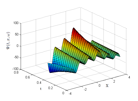
Figure 1. Picture from an animation of Ornstein-Uhlenbeck stochastic process defined by stochastic differential equation (4.1) with initial value problem (4.2)

$>>N=10000;$

$s=1.174;$

$x1=\mbox{ random}(\mbox{'Normal'},0,1,N,1000);$

$A1=[-10,0,0,0,0,0,0,0,0,0,0,0,0,0,0,0,0,0,0,0,0,0];$

$C1=[15,0,3,0,0,0,0,1,0,0,0,0,0,0,0,0,0,0,0,0];$

$D1=[0,0,5,0,15,0,0,0,0,0,0,0,0,0,0,0,0,0,0,0];$

$A10=2;A20=0;C10=1;$

$\mbox{for}~{}k=1:20$

$S1(k)=A10;S2(k)=A20;$

$\mbox{for}~{}n=1:10$

$S1(k)=S1(k)+(-1)^{(}n)*A1(2*n)*k^{(}2*n);$

end

end

$\mbox{for}~{}k=1:20$

$O1(k)=0;$

end

$\mbox{for}~{}k=1:20$

$\mbox{for}n=1:10$

$O1(k)=O1(k)+(-1)^{n}*A1(2*n+1)*k^{(}2*n+1);$

end

end

$[T1,X1]=\mbox{meshgrid}(0:(pi/100):2*pi,-pi:(pi/100):pi);$

$\mbox{for}~{}m=1:N$

$Z1=0.5*C10*exp(T1.*A10)+s*x1(m,1)*((s/sqrt(2*A10))*exp(T1*(-1)*A10).*exp(T1*2*A10)-1);$

$\mbox{for}~{}k=1:20$

$Z1=Z1+C1(k)*exp(T1*S1(k)).*cos(X1.*k).*cos(T1*O1(k))+D1(k)*exp(T1*S1(k)).*cos(X1.*k).*sin(T1*O1(k))+D1(k)*exp(T1*S1(k)).*sin(X1.*k).*cos(T1*O1(k))-$

$C1(k)*exp(T1*S1(k)).*sin(X1.*k).*sin(T1*O1(k))+s*sqrt(2)*x1(m,k+1)*sin(pi*k*(exp(2*A10*T1)-1))/(pi*k);$

end

$\mbox{surf}~{}(X1,T1,Z1)$

drawnow;

$\mbox{pause}(1);$

end

Example 4.2.

Let consider the Ornstein-Uhlenbeck stochastic differential equation

$(4.3)$ $$d\Psi(t,x,\omega)=2\Psi(t,x,\omega)dt-\frac{\partial}{\partial x}\Psi(t,x,\omega)dt+\sigma dW(t,\omega),$$

with initial condition

$(4.4)$ $$\Psi(0,x,\omega)=1/2+5cosx+5cos5x,$$

$$~{}(t,x,\omega)\in[0,\frac{\pi}{7}[\times[-\pi,\pi[\times R^{\infty}.$$

Below we present the programm in Matlab which draw a sample of the size 4 which are results of observations to solutions of the Ornstein-Uhlenbeck stochastic differential equation $(4.3)-(4.4)$ at moment $t=\pi/7$.

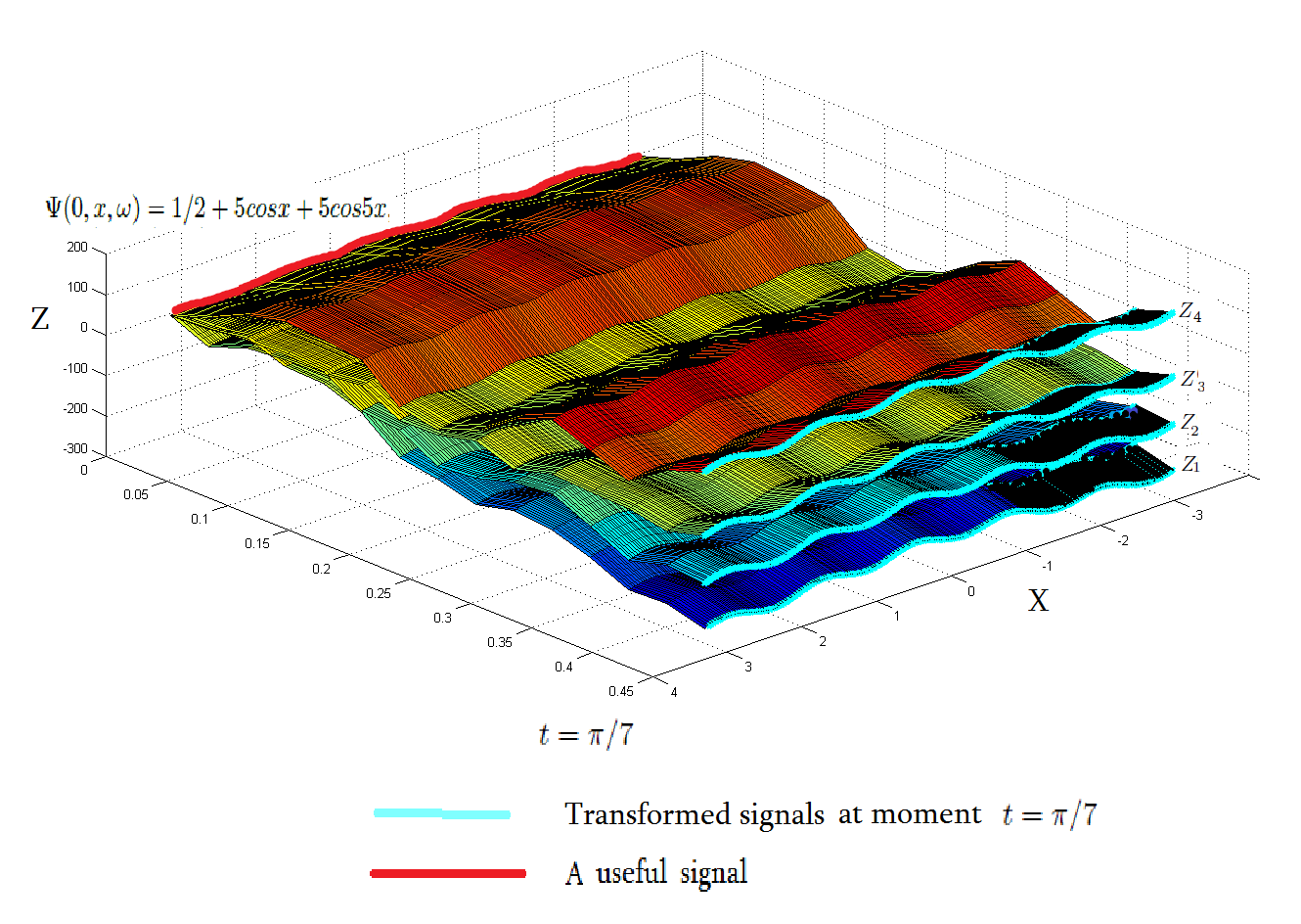
Figure 2. A sample of the size 4 which are results of observations to the solutions of the Ornstein-Uhlenbeck stochastic differential equation (4.3)-(4.4) at moment $t=\pi/7$ when $\sigma=150$

$>>N=4;$

$x1=\mbox{random}(^{\prime}\mbox{Normal}^{\prime},0,1,N,1000);$

$A1=[-1;0;0;0;0;0;0;0;0;0;0;0;0;0;0;0;0;0;0;0;0;0];$

$C1=[5;0;0;0;0;0;0;0;0;0;0;0;0;0;0;0;0;0;0;0];$

$D1=[0;0;0;0;5;0;0;0;0;0;0;0;0;0;0;0;0;0;0;0];$

$A10=2;C10=1;s=150;$

$fork=1:20$

$S1(k)=A10;$

$\mbox{for}~{}n=1:10$

$S1(k)=S1(k)+(-1)^{(}n)*A1(2*n)*k^{(}2*n);$

end

end

$fork=1:20$

$O1(k)=0;$

end

$\mbox{for}~{}k=1:20$

$\mbox{for}~{}n=1:10$

$O1(k)=O1(k)+(-1)^{n}*A1(2*n+1)*k^{(}2*n+1);$

end

end

$[T1,X1]=meshgrid(0:(pi/100):pi/7,-pi:(pi/100):pi);$

$form=1:N$

$Z_{m}=0.5*C10*exp(T1*A10)+(s*x1(1,1)/sqrt(2*A10))*exp(-A10*T1).*(exp(2*A10*T1)-1);$

end

$form=1:N$

$fork=1:20$

$Z_{m}=Z_{m}+C1(k)*exp(T1*S1(k)).*cos(X1.*k).*cos(T1*O1(k))+D1(k)*exp(T1*S1(k)).*cos(X1.*k).*sin(T1*O1(k))+D1(k)*exp(T1*S1(k)).*sin(X1.*k).*cos(T1*O1(k))-$

$C1(k)*exp(T1*S1(k)).*sin(X1.*k).*sin(T1*O1(k))+(s/(sqrt(2*A10)*pi*k))*sqrt(2)*x1(m,k+1)*exp(-A10*T1).*sin(pi*k*(exp(2*A10*T1)-1));$

end

end

$\mbox{surf}(X1,T1,Z_{1})$

hold  on

$\mbox{surf}(X2,T2,Z_{2})$

hold  on

$\mbox{surf}(X3,T3,Z_{3})$

hold  on

$\mbox{surf}(X4,T4,Z_{4})$

hold  off

$>>$

Example 4.3.

Suppose that we have a sample $(Z_{i})_{1\leq i\leq n}\in(FD^{(0)}[-\pi,\pi[)^{n}$ of size $n$. In our simulation, we have that

$$Z_{i}=(\Psi(t_{0},x,\omega^{(i)}))_{x\in[-\pi,\pi[}$$

for $1\leq i\leq n$, where $\omega^{(i)}=(x^{(i)}_{j})_{j\in N}\in{\bf R}^{N}$ is $\gamma$ -uniformly distributed sequence in ${\bf R}$ for each $1\leq i\leq n$. For example, we can put $x^{(i)}_{j}=\Phi^{-1}(\{j\sqrt{p_{i}}\})$, where $p_{i}$ is $i$-th simple natural number for $i\in N$, $j\in N$, $\{\cdot\}$ denotes a fractal part of the real number and $\Phi(t)=\frac{1}{\sqrt{2\pi}}\int_{-\infty}^{t}e^{-\frac{y^{2}}{2}}dy$ for $t\in R$. In that case we can simulate Wiener trajectory $W(t,(x^{(i)}_{j})_{j\in N})$ as follows:

$(4.5)$ $$W(t,(x^{(i)}_{j})_{j\in N})=x^{(i)}_{0}t+\sqrt{2}\sum_{n=1}^{\infty}x^{(i)}_{n}\frac{\sin\pi nt}{\pi n}.$$

Since

$$\sigma\int_{0}^{t_{0}}e^{(t_{0}-\tau)\mathbb{A}}dW(\tau,(x^{(i)}_{j})_{j\in N}))=\frac{\sigma}{2A_{0}}e^{-A_{0}t_{0}}(x^{(i)}_{0}(e^{2A_{0}t_{0}}-1)+$$

$(4.6)$ $$\sqrt{2}\sum_{n=1}^{\infty}x^{(i)}_{n}\frac{\sin(\pi n(e^{2A_{0}t_{0}}-1))}{\pi n}),$$

we can simulate $Z_{i}$ as follows

$$Z_{i}=(\Psi(t_{0},x,(x^{(i)}_{j})_{j\in N}))_{x\in[-\pi,\pi[}=\frac{e^{tA_{0}}c_{0}}{2}+\sum_{k=1}^{\infty}e^{\sigma_{k}t}\Big{(}(c_{k}\cos(\omega_{k}t)+$$

$$d_{k}\sin(\omega_{k}t))\cos(\frac{k\pi x}{l})_{x\in[-\pi,\pi[}+(d_{k}\cos(\omega_{k}t)-c_{k}\sin(\omega_{k}t))\sin(\frac{k\pi x}{l})_{x\in[-\pi,\pi[}\Big{)}+$$

$(4.7)$ $$\frac{\sigma}{2A_{0}}e^{-A_{0}t_{0}}(x^{(i)}_{0}(e^{2A_{0}t_{0}}-1)+\sqrt{2}\sum_{n=1}^{\infty}x^{(i)}_{n}\frac{\sin(\pi n(e^{2A_{0}t_{0}}-1))}{\pi n}).$$

Suppose we want to estimate a useful signal $\Psi_{0}(x)_{x\in[-l,l[}\in FD^{(0)}$ defined by

$(4.8)$ $$\Psi_{0}(x)_{x\in[-\pi,\pi[}=\frac{c_{0}}{2}+\sum_{k=1}^{\infty}c_{k}\cos\Big{(}\frac{k\pi x}{l}\Big{)}_{x\in[-\pi,\pi[}+d_{k}\sin\Big{(}\frac{k\pi x}{l}\Big{)}_{x\in[-\pi,\pi[}.$$

For a function $f\in FD^{(0)}([-\pi,\pi[)$ we put :

$(4.9)$ $$\tilde{c}_{0}(f)=\frac{1}{\pi}\int_{-\pi}^{\pi}f(x)dx;$$

$(4.10)$ $$\tilde{c}_{k}(f)=\frac{1}{\pi}\int_{-\pi}^{\pi}\cos(kx)f(x)dx(k\in\mathbb{N});$$

$(4.11)$ $$\tilde{d}_{k}(f)=\frac{1}{\pi}\int_{-\pi}^{\pi}\sin(kx)f(x)dx(k\in\mathbb{N}).$$

Suppose that all conditions of Theorem 3.1 are satisfied. Then following Theorem 3.1, an estimator $T_{n}$ of the useful signal $\Psi_{0}$ is given by

$$T_{n}((Z_{i})_{1\leq i\leq n})=\frac{e^{-t_{0}A_{0}}\tilde{c}_{0}(\frac{\sum_{i=1}^{n}Z_{i}}{n})}{2}+\sum_{k=1}^{\infty}e^{-\sigma_{k}t_{0}}\Big{(}(\tilde{c}_{k}(\frac{\sum_{i=1}^{n}Z_{i}}{n})\cos(\omega_{k}t_{0})+$$

$$\tilde{d}_{k}(\frac{\sum_{i=1}^{n}Z_{i}}{n})\sin(\omega_{k}t_{0}))\cos(kx)_{x\in[-\pi,\pi[}+(\tilde{d}_{k}(\frac{\sum_{i=1}^{n}Z_{i}}{n})\cos(\omega_{k}t_{0})-$$

$(4.12)$ $$\tilde{c}_{k}(\frac{\sum_{i=1}^{n}Z_{i}}{n})\sin(\omega_{k}t_{0}))\sin(kx)_{x\in[-\pi,\pi[}\Big{)}$$

Our next programm draws results of calculations of the estimate $T_{10}$ of a useful signal when we have a sample of size 10 which are results of observations to the solutions of the Ornstein-Uhlenbeck stochastic differential equation $(4.3)-(4.4)$ at moment $t_{0}=\pi/7$ and $\sigma\in\{150;1500;7500;15000\}.$

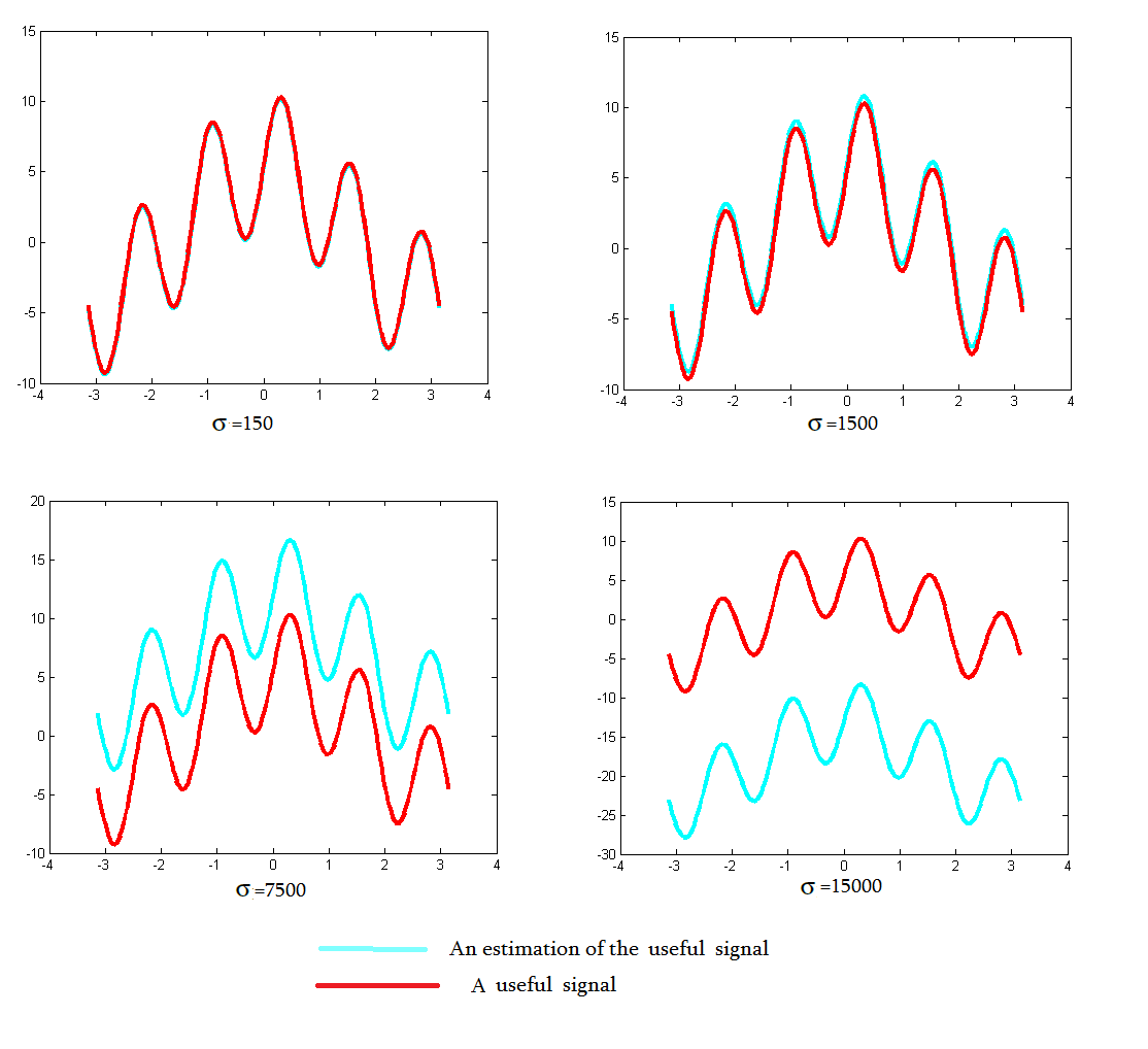
Figure 3. An estimation of the useful signal by using the statistic $T_{10}$ in the Ornstein-Uhlenbeck process (4.3)-(4.4) by the sample of the size $10$ which are results of observations to transformed signals at moment $t_{0}=\pi/7$ when $\sigma\in\{150;1500;7500;15000\}$

$>>N=1000;M=10;s=150;$

$x1=\mbox{ random}(\mbox{'Normal'},0,1,N,1000);$

$A1=[-1,0,0,0,0,0,0,0,0,0,0,0,0,0,0,0,0,0,0,0,0,0];$

$C1=[5,0,0,0,0,0,0,0,0,0,0,0,0,0,0,0,0,0,0,0];$

$D1=[0,0,0,0,5,0,0,0,0,0,0,0,0,0,0,0,0,0,0,0];$

$A10=2;C10=1;$

$\mbox{for}~{}k=1:20$

$S1(k)=A10;S2(k)=A20;$

$\mbox{for}~{}n=1:10$

$S1(k)=S1(k)+(-1)^{n}*A1(2*n)*k^{2*n};$

end

end

$\mbox{for}~{}k=1:20$

$O1(k)=0;$

end

$\mbox{for}~{}k=1:20$

$\mbox{for}~{}n=1:10$

$O1(k)=O1(k)+(-1)^{n}*A1(2*n+1)*k^{2*n+1};$

end

end

$T1=pi/7;$

$X1=-pi:(pi/100):pi;$

$\mbox{for}~{}m=1:M$

$Z_{m}=0.5*C10*exp(T1*A10)+2/sqrt(2*A10)*exp(-A10*T1)*x1(m,1)*(exp(2*A10*T1)-1);$

end

$\mbox{for}~{}m=1:M$

$\mbox{for}~{}k=1:20$

$Z_{m}=Z_{m}+C1(k)*exp(T1*S1(k)).*cos(X1.*k).*cos(T1*O1(k))+D1(k)*exp(T1*S1(k)).*cos(X1.*k).*sin(T1*O1(k))+$

$D1(k)*exp(T1*S1(k)).*sin(X1.*k).*cos(T1*O1(k))-C1(k)*exp(T1*S1(k)).*sin(X1.*k).*sin(T1*O1(k))+$

$s*2/sqrt(2*A10)*exp(-A10*T1)*sqrt(2)*x1(m,k+1)*sin(pi*k*(exp(2*A10*T1)-1))/(pi*k);$

end

end

$W=0;$

$\mbox{for}~{}m=1:M$

$W=W+Z_{m};$

end

$W=W/M;$

$c=0;$

$y=W;$

$\mbox{for}~{}s=1:200$

$c=c+(2/(2*pi*200))*y(s);$

end

$\mbox{for}~{}m=1:20$

$a_{m}=0;$

$b_{m}=0;$

end

$\mbox{for}~{}m=1:20$

$\mbox{for}~{}k=1:200$

$a_{m}=a_{m}+(1/100)*y(k)*cos(m*X1(k));$

$b_{m}=b_{m}+(1/100)*y(k)*sin(m*X1(k));$

end

end

$Y=c*exp(-T1*A10)/2;$

$\mbox{for}~{}k=1:20$

$Y=Y+exp(-S1(k)*T1)*((a_{k}*cos(-O1(k)*T1)+b_{k}*sin(-O1(k)*T1))*cos(k*X1)+(b_{k}*cos(-O1(k)*T1)-a_{k}*sin(-O1(k)*T1))*sin(k*X1))$

end

$Y3=5*cos(X1)+5*sin(5*X1)+C10/2;$

$\mbox{plot}(X1,Y,^{\prime}c^{\prime},X1,Y3,^{\prime}r^{\prime},\mbox{'LineWidth'},3)$

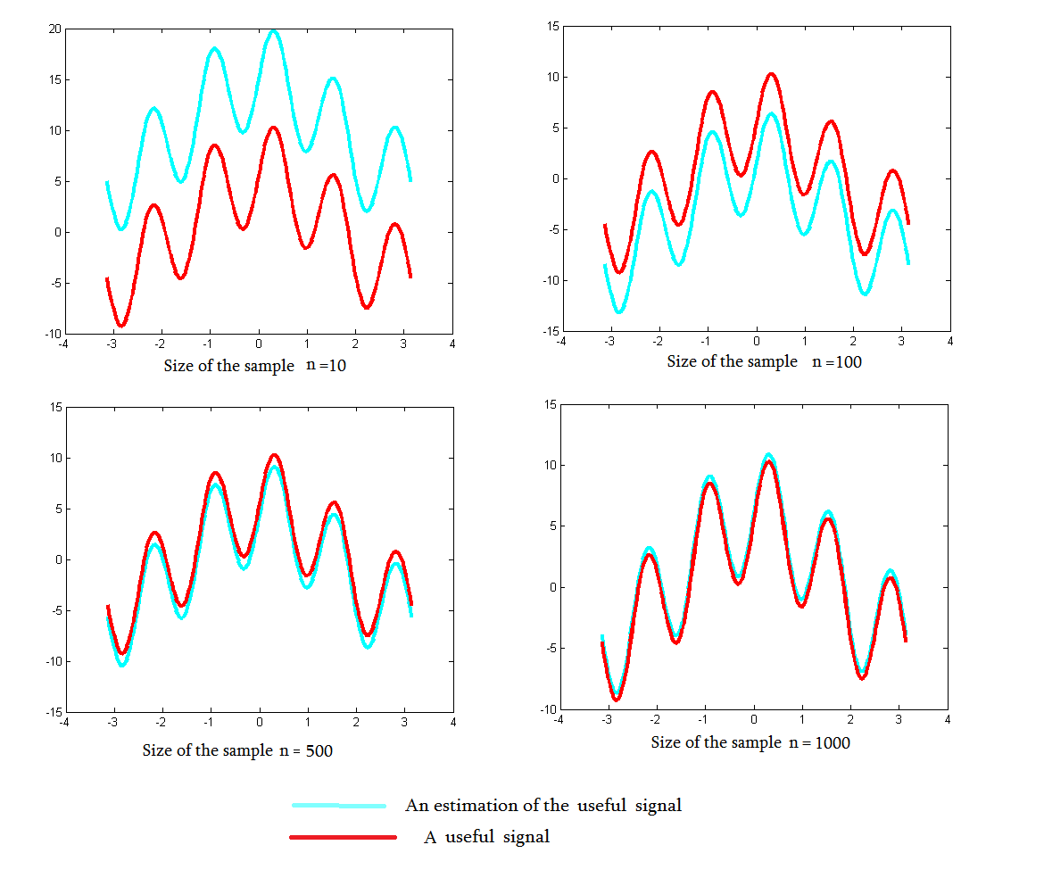
Figure 4. An estimation of the useful signal by using the statistic $T_{n}$ in the Ornstein-Uhlenbeck process (4.5)-(4.6) by the increase of a size of the sample when $\sigma=15000$

5. Discussion and conclusion

If a transmitting process of a useful signal $\theta\in\Theta$ is described by the Ornstein-Uhlenbeck stochastic system (1.1) and we have results of observations $(Z_{k})_{1\leq k\leq n}$ on transformed signals at any moment $t_{0}>0$, then following Theorem 3.1, by using the statistic $T_{n}$ we can restore $\theta$.

Programs in Matlab prepared in the present paper can be described as follows:

(i) A programm in Matlab from Example 4.1 demonstrates animation of a particular case of the Ornstein-Uhlenbeck stochastic system (1.1) which are defined by (4.1)-(4.2)(see Figure 1).

(ii) A programm in Matlab from Example 4.2 draws and presents a sample $(Z_{k})_{1\leq k\leq n}$ of the size $n$ which consists from results of observations to $n$ independent transformed signals at moment $t=\pi/7$ when a transmitting process of a useful signal $\theta$ is described by the Ornstein-Uhlenbeck stochastic system (1.1) defined by (4.3)-(4.4) (see Example 4.2 and Figure 2 for which $n=4$ ).

(iii) A programm in Matlab from Example 4.3 draws the value of the statistic $T_{n}$ (which is in $C[-\pi,\pi[$) calculated for sample $(Z_{k})_{1\leq k\leq n}$ of the size $n$ which consists from results of observations to $n$ independent transformed signals at moment $t=\pi/7$ when a transmitting process of a useful signal $\theta$ is described by the Ornstein-Uhlenbeck stochastic system (1.1) defined by (4.5)-(4.6). (see Example 4.3 and Figure 3 ).

From Figure 3 we see that the reduction of the parameter $\sigma$ in (4.3), for the fixed size of the sample(here, $n=10$) increases the accuracy of the estimation of the useful signal which seems naturally.

Similarly, from Figure 4 we see that an increase of the size of the sample, for a fixed big value of the parameter $\sigma$ in (4.3)( here, $\sigma=1500$ ), also increases the accuracy of the estimation of the useful signal which do not contradicts to the result of Theorem 3.1.

References

• [1] Gantmacher F. R.: Theorie des matrices. Tome 1: Theorie gen- erale. (French) Traduit du Russe par Ch. Sarthou. Collection Universitaire de Mathematiques, No. 18 Dunod, 1966.
• [2] Garbaczewski, P., Olkiewicz, R.: Ornstein-Uhlenbeck-Cauchy process, J. Math. Phys., 41(2000), 6843–6860.
• [3] Gillespie, D. T.: Exact numerical simulation of the Ornstein-Uhlenbeck process and its integral. Physical review E 54, (1996). no. 2: 2084–2091.
• [4] Ornstein, L. S., Uhlenbeck, G. E.: On the Theory of the Brownian Motion. Physical Review 36,(1930). no. 5: 823. doi:10.1103/PhysRev.36.823.
• [5] Labadze, L.,Pantsulaia, G.: Estimation of the parameters of the Ornstein-Uhlenbeck’s process. https://arxiv.org/pdf/1608.04507v3.pdfdestination
• [6] Pantsulaia, G. R., Giorgadze, G.P.: On a Linear Partial Differential Equation of the Higher Order in TwoVariables with Initial Condition Whose Coefficients are Real-valued Simple Step Functions, J. Partial Diff. Eqs., 29 (2016) . No. 1, 1-13
• [7] Labadze, L., Saatashvili, G., Pantsulaia, G.: Infinite-sample consistent estimations of parameters of the Wiener process with drift. https://arxiv.org/pdf/1611.01119v2.pdfdestination
• [8] Protter, P.: Stochastic integration and differential equations, Springer-Verlag, Berlin, 2004.
• [9] Shiryaev, A.N.: Probability (in Russian), Izd.β€œNauka”, Moscow, 1980.
• [10] Smith, William.: On the Simulation and Estimation of the Mean-Reverting Ornstein-Uhlenbeck Process, Especially as Applied to Commodities Markets and Modelling, Verson 1.01 (February), 2010. https://commoditymodels.files.wordpress.com/2010/02/estimating-the-parameters-of-a-mean-reverting-ornstein-uhlenbeck-process1.pdfdestination
• [11] Ibramkhallilov, I.Sh., Skorokhod, A.V.: On well–off estimates of parameters of stochastic processes (in Russian), Kiev, 1980.