A numerical scheme for the compressible low-Mach number regime of ideal fluid dynamics

Abstract

Based on the Roe solver a new technique that allows to correctly represent low Mach number flows with a discretization of the compressible Euler equations was proposed in miczek2015a . We analyze properties of this scheme and demonstrate that its limit yields a discretization of the continuous limit system. Furthermore we perform a linear stability analysis for the case of explicit time integration and study the performance of the scheme under implicit time integration via the evolution of its condition number. A numerical implementation demonstrates the capabilities of the scheme on the example of the Gresho vortex which can be accurately followed down to Mach numbers of $\sim 10^{-10}$.

1 Introduction

This paper concerns itself with finite volume schemes for the compressible Euler equations, in regimes where the Mach number may become both high and quite low. When the Mach number is of order one, modern shock capturing methods are able to resolve discontinuities and other complex structures with high numerical resolution. For the Mach number going to zero the solutions to the compressible Euler equations

$$\partial_{t}\varrho+\nabla\cdot(\varrho\mathbf{v}) =0$$ (1)

$$\partial_{t}(\varrho\mathbf{v})+\nabla\cdot\left(\varrho\mathbf{v}\otimes\mathbf{v}+p\cdot\mathbb{1}\right) =0$$ (2)

$$\partial_{t}E+\nabla\cdot[\mathbf{v}(E+p)] =0$$ (3)

tend to the solutions of the incompressible Euler equations. This has been demonstrated by e.g. klainerman1981a ; metivier2001a . They found that the various functions (pressure, density, etc.) converge to those encountered in the incompressible setting at different rates in the Mach number. A numerical method needs to take account of this.

For the compressible Euler equations the CFL stability criterion of an explicit time discretization requires the time step to be very small for small Mach numbers. This is due to the fact that in this regime the sound waves are much faster than the advection of the flow. Additionally to this stiffness in time, shock-capturing methods show an excessive diffusion which completely deteriorates the solution when the methods are applied to flows with low Mach numbers.

In order to deal with these problems in the literature one finds two approaches:

• In one approach the flux function of the finite volume method is modified. The idea is to adapt the flux to the low Mach situation. Recent suggestions of flux modification include dellacherie2010a ; rieper2011a ; osswald2015a ; chalons2016a . This is a method that was initially proposed by Eli Turkel (turkel1999a ) for the calculation of steady state flows and was subsequently extended. These methods however are not well suited for flows where low-Mach flows occur simultaneously with flows that have speeds comparable to the sound speed.

• In another approach Klein (klein1995a ) devised an algorithm that keeps track of different orders in the asymptotic expansion of the pressure. The idea is to split the system into two parts. One of them involves a slow, nonlinear and conservative hyperbolic system adequate for the use of modern shock capturing methods mentioned above, and the other is a linear hyperbolic system which contains the stiff acoustic dynamics, which is to be solved implicitly. Recent developments for all-speed schemes of this sort are cordier2012a ; haack2012a ; degond2011a . In summary, this leads to a hybrid scheme, partly implicit in time, partly explicit.

In this paper we are inspired by the first approach. It is based on a recently published astrophysical paper miczek2015a , where the authors propose a new hydrodynamics solver based on modifying the diffusion matrix of the Roe scheme. In spirit this is not dissimilar to turkel1999a , where these modifications were referred to as flux-preconditioning for historical reasons. In more extreme astrophysical situations, however, the schemes proposed there may fail. miczek2015a demonstrated that the flux function resulting from previous preconditioning techniques may show inconsistencies in certain applications. With their new scheme a consistent scaling is achieved.

Since this new technique may be useful for applications outside the astrophysical context, in this paper we follow up on the approach taken by miczek2015a and analyze its properties in detail. The requirements for an all Mach number finite volume scheme, inferred from the limit of the continuous system, are

1. the numerical method for the compressible Euler equations converges formally to a discretization of the incompressible equations

2. the numerical evolution of the kinetic energy near the incompressible regime is independent of the Mach number

In addition for an efficient numerical method we require

1. linear stability of the scheme when subject to explicit time integration

2. efficient implicit time integration

The first two requirements are inspired by the properties of the limit at continuous level which will be formulated in Sect. 2. After introducing a discretization of the Euler equations these requirements will be given a shape that is reasonable for numerical applications. In Sect. 3 we give a more extended motivation for the form of the proposed modification of the flux function. For this method, the requirement (i) from above is investigated in Sect. 4 by pursuing the question of whether the technique qualifies as an asymptotic-preserving scheme and whether additionally properties beyond a consistent discretization of the limit equations are needed. With numerical experiments we demonstrate that our scheme yields satisfactory results for flows down to very low Mach numbers, thus giving evidence that it complies with the above requirement (i) and (ii). Because we only modify the diffusion matrix affecting solely the spatial discretization of the equation, we initially employ the method of lines. For practical implementations, this raises the question of an appropriate strategy for time discretization. miczek2015a applied their method in both explicit and implicit time discretization. We discuss stability of the scheme in explicit time discretization in Sect. 5, consistent with requirement (iii), and comment on its efficiency in implicit time discretization, which allows to cover extended periods of time, in Sect. 6 (requirement (iv)).

2 Fluid dynamics in the low Mach number limit

The solutions to

$$\partial_{t}\varrho+\nabla\cdot(\varrho{\mathbf{v}}) =0$$ (4)

$$\partial_{t}(\varrho\mathbf{v})+\nabla\cdot\left(\varrho{\mathbf{v}}\otimes\mathbf{v}+\frac{p}{M^{2}}\cdot\mathbb{1}\right) =0$$ (5)

$$\partial_{t}E+\nabla\cdot\left[\mathbf{v}(E+p)\right] =0$$ (6)

tend to solutions of the incompressible Euler equations as $M\in\mathbb{R}^{+}$ tends to zero, i.e. in the limit of low Mach numbers ebin1977a ; klainerman1981a ; ukai1986a ; asano1987a ; isozaki1987a ; kreiss1991a ; schochet1994a ; metivier2001a . This can formally be seen by expanding all quantities as series in $M$, e.g. for the pressure this would give

$$p(x,t)=p^{(0)}(x,t)+Mp^{(1)}(x,t)+M^{2}p^{(2)}(x,t)+\mathcal{O}(M^{3}).$$ (7)

Inserting these into the above equations, collecting order by order and assuming impermeable boundaries gives

$$p^{(0)} =\mathrm{const},$$ (8)

$$p^{(1)} =\mathrm{const},$$ (9)

$$(\nabla\cdot\mathbf{v})^{(0)} =0,$$ (10)

and

$$\partial_{t}\varrho^{(0)}+\mathbf{v}^{(0)}\cdot\nabla\varrho^{(0)} =0,$$ (11)

$$\partial_{t}\mathbf{v}^{(0)}+(\mathbf{v}^{(0)}\cdot\nabla)\mathbf{v}^{(0)}+\nabla p^{(2)}/\varrho^{(0)} =0.$$ (12)

These equations describe incompressible flows. Conditions (8), (9) and (10) are true for every time. Initial data that fulfill them are called well-prepared. Not well-prepared initial data may lead to an incompressible flow as well, but then an initial disturbance is produced.

The equation for the kinetic energy $E_{\text{kin}}=\frac{1}{2}\varrho|\mathbf{v}|^{2}$ can be rewritten as

$$\partial_{t}E_{\text{kin}}+\nabla\cdot\left[\mathbf{v}\left(E_{\text{kin}}+\frac{p}{M^{2}}\right)\right] =\frac{p}{M^{2}}\nabla\cdot\mathbf{v}.$$ (13)

The source term vanishes for incompressible flows and in this case the kinetic energy becomes a conserved quantity. For compressible flows, this is true in the limit $M\to 0$ as well, despite of $\frac{\nabla\cdot v}{M^{2}}\not\in\mathcal{O}(M)$. Expanding the quantities and using (8) and (9) makes the terms proportional to $\frac{1}{M}$ or $\frac{1}{M^{2}}$ cancel and gives

$$\partial_{t}E_{\text{kin}}+\nabla\cdot\left[\mathbf{v}\left(E_{\text{kin}}+p^{(2)}\right)\right] =p^{(2)}\nabla\cdot\mathbf{v}+\mathcal{O}(M).$$ (14)

Now the source term indeed is $\mathcal{O}(M)$ and the kinetic energy can be seen to become a conserved quantity in the limit $M\to 0$.

We are thus led to phrase the requirements (i) and (ii) from the Introduction in a way as they hold at continuous level:

1. If the initial data for the compressible, homogeneous Euler equations are chosen to have spatial pressure fluctuations scale with $\mathcal{O}(M^{2})$ and the divergence of the velocity field scale with $\mathcal{O}(M)$, then the solution converges to the solution of the incompressible Euler equations in the limit $M\to 0$, with only these pressure fluctuations playing the role of the dynamic pressure.

2. For solutions to the compressible, homogeneous Euler equations in the low Mach number limit, the total kinetic energy is conserved.

They will be stated again in Section 3 in a form adapted to the discrete system. They will thus become requirements for a numerical scheme to be able to capture flows in the low Mach number regime.

3 Spatial discretization and modification of the diffusion matrix

3.1 Finite volume schemes for conservation laws in the low Mach limit

Consider a system of conservation laws

$$\partial_{t}\mathbf{U}+\partial_{x}\vec{F}^{(x)}(\mathbf{U})+\partial_{y}\vec{F}^{(y)}(\mathbf{U})+\partial_{z}\vec{F}^{(z)}(\mathbf{U}) =0$$ (15)

with $\mathbf{U}$ being the vector of conserved quantities ($\mathbf{U}=(\varrho,\varrho\vec{v},E)^{\text{T}}$ in the case of the Euler equations) and $\vec{F}^{(x)}$, $\vec{F}^{(y)}$, $\vec{F}^{(z)}$ the flux in $x$-, $y$- and $z$-direction, respectively.

Its numerical solution of the compressible Euler equations (1)–(3) is achieved by applying the Godunov method on a Cartesian computational grid with a uniform spacing $\Delta x$, $\Delta y$, $\Delta z$. The conserved quantities stored in a cell $(i,j,k)$ are denoted by $\mathbf{U}_{i,j,k}$, and a numerical flux through the interface between cells $(i,j,k)$ and $(i+1,j,k)$ by $\mathbf{F}^{(x)}_{i+1/2,j,k}$. Written as a semi-discrete system the finite volume scheme amounts to

$$\frac{\partial}{\partial t}\mathbf{U}_{i,j,k}+\frac{1}{\Delta x} \left(\mathbf{F}^{(x)}_{i+1/2,j,k}-\mathbf{F}^{(x)}_{i-1/2,j,k}\right)+$$ (16)

$$\frac{1}{\Delta y} \left(\mathbf{F}^{(y)}_{i,j+1/2,k}-\mathbf{F}^{(y)}_{i,j-1/2,k}\right)+$$ (17)

$$\frac{1}{\Delta z} \left(\mathbf{F}^{(z)}_{i,j,k+1/2}-\mathbf{F}^{(z)}_{i,j,k-1/2}\right)=0.$$ (18)

It was suggested by Roe roe1981a to choose the numerical flux as

$$\mathbf{F}_{l+1/2}=\frac{1}{2} \left[\mathbf{F}\left(\mathbf{U}^{\text{L}}_{l+1/2}\right)+\mathbf{F}\left(\mathbf{U}^{\text{R}}_{l+1/2}\right)-\left|A_{\text{Roe}}\right|\left(\mathbf{U}^{\text{R}}_{l+1/2}-\mathbf{U}^{\text{L}}_{l+1/2}\right)\right],$$ (19)

with the matrix $A_{\text{Roe}}$ resulting from the solution of a linearized Riemann problem at the interface of the computational cells. It is the absolute value of the Jacobian $A$, performed on the eigenvalues, and evaluated in the Roe-average state. This term ensures upwinding and introduces an artificial viscosity that stabilizes the scheme. The indices L and R denote the states to the left and to the right of the cell interface as determined from an appropriate reconstruction procedure. In multi-dimensional context this flux is applied direction by direction. One may introduce other matrices instead of $|A_{\text{Roe}}|$, and we will refer to them as diffusion, or upwind artificial viscosity matrices.

As argued in Ref. miczek2015a , the problem arising for this approach in the low Mach number limit is that the upwind artificial viscosity dominates all the other terms in the limit of small Mach numbers even if the initial data are well-prepared. In particular it excites spatial pressure fluctuations $\mathcal{O}(M)$. One thus is led to require for a numerical scheme able to maintain low Mach number flows:

1. Considering the limit $M\to 0$, and having initial data for the compressible, homogeneous Euler equations chosen to have spatial pressure fluctuations scale with $\mathcal{O}(M^{2})$, then this shall hold for the data at late times as well.

2. Numerical solutions to the compressible, homogeneous Euler equations in the low Mach number limit and with fixed discretization shall display a (numerical) dissipation of kinetic energy that is $\mathcal{O}(1)$ in the limit $M\to 0$. In particular this means that the dissipation shall not grow with decreasing $M$.

These are modified versions of the findings mentioned in Sect. 2, reinterpreted in regard to numerical methods. The emphasis on a fixed discretization is due to the ubiquitous observation that with usual finite volume methods for fixed $M$ the dissipation is effectively reduced by increasing the spatial resolution. However this is neither efficient with respect to the invested computation time nor does it touch the root of the problem, the artefacts just reappearing on finer scales again.

For numerical methods we require additionally

1. linear stability under explicit time integration

2. efficient implementation of implicit time integration

After the discussion of the proposed scheme in this Section, we address (i) and (ii) in Section 4, (iii) in Section 5 and (iv) in Section 6.

The central flux,

$$\vec{F}_{l+1/2}=\frac{1}{2}\left[\vec{F}(\vec{U}^{L}_{l+1/2})+\vec{F}(\vec{U}^{R}_{l+1/2})\right].$$ (20)

would be a choice complying with the low Mach number limit, but it lacks stability in explicit time discretization.

Numerical tests, as shown in Figure 3 of miczek2015a , suggest that it is stable in the implicit case. A small growth in kinetic energy is observed, which is, while not being in contradiction with the basic conservation laws, in contradiction with thermodynamics and therefore less suited to many practical applications.

Replacing $\left|A_{\text{Roe}}\right|$ by the modified diffusion matrix

$$P^{-1}\left|PA\right|$$ (21)

with $P$ a suitable invertible matrix, and $A$ the Jacobian, is observed (turkel1999a ) to improve the numerical solutions in the low Mach number regime. Miczek et al. miczek2015a argue that this is because $P$ can be chosen to correct the scaling behavior with low Mach number found in the diffusion matrix. For historical reasons $P$ is called preconditioning matrix; we will refer to it as the modifying matrix. A widely used one is due to Weiss and Smith weiss1995a , in primitive variables

$$P_{\text{prim}}=\begin{pmatrix}1&0&0&0&\frac{\mu^{2}-1}{c^{2}}\\ 0&1&0&0&0\\ 0&0&1&0&0\\ 0&0&0&1&0\\ 0&0&0&0&\mu^{2}\end{pmatrix},$$ (22)

with the parameter

$$\mu=\min[1,\max(M_{\text{loc}},M_{\text{cut}})],$$ (23)

which should scale with the local Mach number $M_{\text{loc}}$. Its lower limit, $M_{\text{cut}}$, avoids singularity of the matrix.

It corrects the scaling behavior of almost all entries in the diffusion matrix. Indeed, when used with the homogeneous Euler equations it shows very low, Mach number independent dissipation in the low Mach limit. However, when integrated implicitly in time, this scheme displays unsatisfactory behavior of the condition number as discussed later.

3.2 Low Mach modifications in presence of gravity source terms

A problem with the particular choice (22) of the dissipation matrix arises if it is used in the presence of certain source terms, e.g. gravity. Here the lowest order in the expansion of the pressure in powers of $M$ is not constant. The diffusion matrix obtained when using (22) has an entry $\mathcal{O}(1/M^{2})$ in the energy row. Therefore with a spatially varying background this introduces strong diffusion. An example in which such configurations arise are hydrostatic equilibria in presence of gravity. Here the rescaled Euler equations, (4)–(6), change to

$$\partial_{t}\varrho+\nabla\cdot(\varrho\mathbf{v}) =0,$$ (24)

$$\partial_{t}(\varrho\mathbf{v})+\nabla\cdot\left(\varrho\mathbf{v}\otimes\mathbf{v}+\frac{p}{M^{2}}\cdot\mathbb{1}\right) =\frac{\varrho}{\mathit{Fr}^{2}}\mathbf{g},$$ (25)

$$\partial_{t}E+\nabla\cdot[\mathbf{v}(E+p)] =\frac{M^{2}}{\mathit{Fr}^{2}}\varrho\mathbf{g}\cdot\mathbf{v}.$$ (26)

The nondimensional Froude number $\mathit{Fr}$ appears in presence of gravity source terms. For the purposes of this article we only consider the case of $\mathit{Fr}=M$.

This new system admits static solutions (stationary and with $\mathbf{v}=0$) called hydrostatic equilibria which are governed by the condition $\nabla p=\varrho\mathbf{g}$.

To point out and compare the properties of the numerical schemes in presence of this source term, consider a special but important solution in one spatial dimension. In the case of a constant temperature $T$, spatially and temporally constant $\mathbf{g}=-g\mathbf{e}_{x}$ pointing into the negative $x$-direction and the ideal gas equation of state, hydrostatic equilibrium has the form

$$\varrho(x)=\varrho_{0}\exp\left(-\frac{gx}{T}\right),\quad p(x)=\varrho(x)T,\quad\varrho_{0}:=\varrho(0)$$ (27)

We can compute the discrete fluxes using (21) on a uniform grid with spacing $\Delta x$ using constant reconstruction. The change in grid cell $i$ is given by

$$-\partial_{t}\mathbf{U}_{i}=\begin{pmatrix}0\\ \frac{p_{i+1}-p_{i-1}}{2\Delta xM^{2}}+\varrho_{i}g\\ 0\end{pmatrix}+\frac{1}{2\Delta x}\left(-\mathbf{D}_{i+1/2}+\mathbf{D}_{i-1/2}\right).$$ (28)

with $\mathbf{D}_{i+1/2}=(P^{-1}|PA)_{\text{Roe},i+1/2}\;(\mathbf{U}_{i+1}-\mathbf{U}_{i})$.

For the first expression, which corresponds to the central flux, Eq. (20), we get

$$\frac{p_{i+1}-p_{i-1}}{2\Delta x} =\frac{\varrho_{0}T}{2\Delta x}\left[\exp\left(-\frac{g(i+1)\Delta x}{T}\right)-\exp\left(-\frac{g(i-1)\Delta x}{T}\right)\right]$$ (29)

$$=-\varrho_{i}g\left[1+\frac{g^{2}\Delta x^{2}}{6T^{2}}+\mathcal{O}\left({\Delta x^{4}}\right)\right].$$

which cancels with the cell-centered discretization of gravity up to order of $\Delta x^{2}$.

The effect of the numerical dissipation term $\mathbf{D}_{i\pm 1/2}$ can most conveniently be evaluated in primitive variables ($\varrho,\vec{v},p$). For the modifying matrix $P$ in Eq. (22) the contribution is

$$\frac{\mathbf{D}_{i+1/2}}{2\Delta x}=\begin{pmatrix}1\\ 0\\ c^{2}\end{pmatrix}\frac{\Delta p}{2\Delta xcM_{\text{cut}}},$$ (30)

with $\Delta p=p_{i+1}-p_{i}$ and the local speed of sound $c=\sqrt{\gamma p/\varrho}$ with the $\gamma$ from Eq. (95). As we consider hydrostatic solutions here, the bounded local Mach number $\mu$ (23) was set to its lower limit $M_{\text{cut}}$. Recall that $M_{\text{cut}}$ is normally chosen to a value well below the Mach number in the considered flow field, just large enough to avoid infinite values when dividing by $\mu$ in zero-velocity regions, while maintaining the positive effect of the modification of the diffusion matrix at reasonably low Mach numbers. Eq. (30) reveals a fundamental problem when using the matrix (22) – its contribution becomes extremely large in regions with very low Mach numbers if a pressure gradient is present. While this is generally not the case in low Mach number flows when the homogeneous Euler equations are solved, it can happen, if gravity or other source terms are involved.

Because of these problems, Miczek et al. miczek2015a suggested a new modifying matrix $P$. In entropy variables it takes the form,

$$P_{\text{entr}}=\begin{pmatrix}1&n_{x}\delta&n_{y}\delta&n_{z}\delta&0\\[4.30554pt] -n_{x}\delta&1&0&0&0\\[4.30554pt] -n_{y}\delta&0&1&0&0\\[4.30554pt] -n_{z}\delta&0&0&1&0\\[4.30554pt] 0&0&0&0&1\end{pmatrix},$$ (31)

with $\delta=\frac{1}{\min(1,\max(M_{\text{loc}},M_{\text{cut}}))}-1$. In primitive variables it is

$$P_{\text{prim}}=\begin{pmatrix}1&n_{x}\frac{\varrho\delta M}{c}&n_{y}\frac{\varrho\delta M}{c}&n_{z}\frac{\varrho\delta M}{c}&0\\[4.30554pt] 0&1&0&0&-n_{x}\frac{\delta}{\varrho cM}\\[4.30554pt] 0&0&1&0&-n_{y}\frac{\delta}{\varrho cM}\\[4.30554pt] 0&0&0&1&-n_{z}\frac{\delta}{\varrho cM}\\[4.30554pt] 0&n_{x}\varrho c\delta M&n_{y}\varrho c\delta M&n_{z}\varrho c\delta M&1\end{pmatrix}.$$ (32)

As for the modifying matrix from Eq. (22), the definition of $\delta$ ensures that the scheme reverts back to the original Roe scheme when the local Mach number reaches 1. Miczek et al. miczek2015a show that the scaling with $M$ of the diffusion matrix of this scheme is fully consistent with the flux Jacobian. The flux at any cell edge is given, similarly to (19) by

$$\mathbf{F}_{l+1/2}=\frac{1}{2} \left[\mathbf{F}\left(\mathbf{U}^{\text{L}}_{l+1/2}\right)+\mathbf{F}\left(\mathbf{U}^{\text{R}}_{l+1/2}\right)-P^{-1}\left|PA\right|\left(\mathbf{U}^{\text{R}}_{l+1/2}-\mathbf{U}^{\text{L}}_{l+1/2}\right)\right]$$

We can perform the analysis of the discretized fluxes in hydrostatic equilibrium for this solver, too. Equation (29) is identical for both. Instead of the dissipation term from Eq. (30), we get in primitive variables

$$\frac{\mathbf{D}_{i+1/2}}{2\Delta x}=\begin{pmatrix}M_{\text{cut}}c^{-1}\\ \frac{M_{\text{cut}}-1}{\varrho M}\\ cM_{\text{cut}}\end{pmatrix}\frac{\Delta p}{2\Delta xM\sqrt{1-2M_{\text{cut}}+2M_{\text{cut}}^{2}}}.$$ (33)

This expression overcomes the problems of the preconditioner in Eq. (22) because its dissipation term does not grow when lowering $M_{\text{cut}}$. Therefore the new method avoids the problems encountered for previously suggested modification matrices in presence of gravity.

Solutions to the Euler equations augmented by a gravity source term need not in general be or converge to a static equilibrium. However there are indeed a lot of interesting applications related to such equilibria. The ability of a scheme to preserve them up to machine precision is a challenging additional requirement, an implementation of which however is not the topic of this paper but subject of ongoing work.

4 Asymptotic behavior of the numerical method

4.1 Asymptotic analysis of the semi-discrete scheme

It has been demonstrated in miczek2015a that the new way of modifying the diffusion matrix (Eq. (31) or (32)) ensures that the diffusive part

$$P^{-1}\left|PA\right|\left(\mathbf{U}^{\text{R}}_{l+1/2}-\mathbf{U}^{\text{L}}_{l+1/2}\right)$$

does not dominate the numerical flux function at low Mach numbers. In the context of asymptotic preserving schemes it has been found useful to analyze the limit of the discrete system, in a way analogous to what has been done in Sect. 2 in the continuous case. With, for simplicity, a piecewise constant reconstruction, the numerical flux in $x$-direction is given by

$$\mathbf{F}_{i+\frac{1}{2}}=\frac{1}{2}\left[\mathbf{F}(\mathbf{U}_{i+1})+\mathbf{F}(\mathbf{U}_{i})\right]-\frac{1}{2}P^{-1}|PA|(\mathbf{U}_{i+1}-\mathbf{U}_{i}),$$ (34)

where $P^{-1}|PA|$ is evaluated in the Roe state, and $A$ is the Jacobian in $x$-direction (indices for the other directions have been dropped for better readability). The fluxes through the other interfaces can be obtained analogously.

Taking $\delta\in\mathcal{O}\left(\frac{1}{M}\right)$, by construction the leading order terms in $M$ of the diffusion matrix are the same as in the Jacobian (miczek2015a ). In the basis of conserved variables one finds

$$P^{-1}|PA| =\frac{1}{M^{2}}\left(\begin{array}[]{ccccc}0&0&0&0&0\\ 0&0&0&0&\gamma-1\\ 0&0&0&0&0\\ 0&0&0&0&0\\ 0&0&0&0&0\end{array}\right)+\mathcal{O}(1).$$ (40)

A conservative semi-discrete scheme with flux (34) then is

$$0 =\partial_{t}\mathbf{U}_{i}+\frac{\mathbf{F}_{i+\frac{1}{2}}-\mathbf{F}_{i-\frac{1}{2}}}{\Delta x}+\text{ fluxes through other interfaces}$$

and to highest order

$$0 =\partial_{t}\mathbf{U}_{i}+\frac{1}{2\Delta x}\left[\frac{1}{M^{2}}\left(\begin{array}[]{c}0\\ p_{i+1}-p_{i-1}\\ 0\\ 0\\ 0\end{array}\right)-\frac{\gamma-1}{M^{2}}\left(\begin{array}[]{c}0\\ E_{i+1}-2E_{i}+E_{i-1}\\ 0\\ 0\\ 0\end{array}\right)\right]+\mathcal{O}({M})$$

The two lowest orders can be simplified (for $\ell=0,1$ one has $p^{(\ell)}=(\gamma-1)E^{(\ell)}$) to formally yield in the limit $M\to 0$:

$$p^{(\ell)}_{i}-p^{(\ell)}_{i-1}=0\qquad\ell=0,1$$ (41)

The rest of the asymptotic analysis is done with the $\mathcal{O}(1)$ equations, which due to the consistency of the scheme give consistent discretizations of the remaining equations in the limit $M\to 0$.

Equation (41) for the Roe solver is, as has been discussed in guillard1999a ; guillard2004a

$$\frac{p^{(0)}_{i+1}-p^{(0)}_{i-1}}{\Delta x} =0$$ (42)

$$\frac{p^{(1)}_{i+1}-p^{(1)}_{i-1}}{\Delta x} =\Delta x\cdot(\text{terms involving $2^{\text{nd}}$ derivatives of $\varrho$, $v$, $e$})+\mathcal{O}(\Delta x^{2}).$$ (43)

Even though it is also a discretization of $\nabla p^{(\ell)}=0$, it is not a good approximation for finite values of $\Delta x$ – contrary to (41). As is well-known it is always possible to cure the low Mach number problems by increasing the resolution. This however, as mentioned above, is both impractical and unnecessary.

In view of the findings we expect our scheme to have pressure perturbations $\mathcal{O}(M^{2})$, consistently with requirement (i) from Sect. 3.

4.2 Numerical results

We demonstrate this result with numerical experiments in which we simulate a Gresho-vortex setup gresho1990a . This is an example of a stationary, incompressible rotating flow around the origin in two spatial dimensions:

$$\vec{v} =\vec{e}_{\phi}\cdot\begin{cases}5r&r<0.2\\ 2-5r&r<0.4\\ 0&\text{else}\end{cases}$$ (44)

$$p =\begin{cases}p_{\text{c}}+\frac{25}{2}r^{2}&r<0.2\\ p_{\text{c}}+4\ln(5r)+4-20r+\frac{25}{2}r^{2}&r<0.4\\ p_{\text{c}}+4\ln 2-2&\text{else}\end{cases}$$ (45)

with the uniform density $\varrho=1$ and the pressure in the vortex center $p_{\text{c}}=\frac{1}{\gamma M^{2}}-\frac{1}{2}$. Also $r=\sqrt{x^{2}+y^{2}}$ and $\vec{e}_{\phi}$ is the azimuthal unit vector in two-dimensional polar coordinates.
In the compressible setting the flow can be endowed with different maximum Mach numbers by varying the parameter $M$ in the value of the central pressure. Therefore this is an example of a family of solutions, parametrized by a real number $M$, such that $M_{\text{loc}}$ scales asymptotically as $M$ in the limit $M\to 0$. Here all quantities are understood to be non-rescaled, and one observes for example that $p=\frac{1}{M^{2}}(\tilde{p}^{(0)}+M\tilde{p}^{(1)}+\ldots)$ and so on.

The setup and the employed numerical method are identical to those presented in Ref. miczek2015a . For the numerical solution, a fully discretized scheme is necessary and we chose an implicit time discretization with an advective CFL criterion to determine the time step size (see Sec. 6). A piecewise linear MUSCL-like reconstruction without limiters is used vanleer1979a ; toro2009a .

As stated above, our goal is to devise a scheme that represents low Mach number flows well at low numerical resolution. Therefore, the Gresho vortex is set up on a grid with only $40\times 40$ computational cells. We follow the flow over one full revolution of the vortex and show the results for maximum Mach numbers down to $10^{-10}$ in Fig. 1. With the Miczek scheme miczek2015a , the vortex is retained in the simulations even at the lowest Mach numbers. This contrasts the result obtained with a conventional Roe-type flux function in which the vortex is significantly blurred after one full revolution at a maximum Mach number of $10^{-2}$ and completely destroyed for maximum Mach numbers below $10^{-3}$ as seen in Fig. 3 and miczek2015a .

The evolution of the total kinetic energy in the simulation domain is shown in Fig. 2 and Table 1. Although the kinetic energy reduces by about 1.3 per cent over one revolution of the vortex in our setup, this loss is independent of the Mach number of the flow. This is very much in contrast to conventional schemes, whose dissipation rate of kinetic energy increases excessively the lower the Mach numbers get.

At high Mach numbers of about $10^{-1}$ the proposed scheme performs similarly to conventional ones. In view of the results one is however led to the observation that it is at the same time able to reproduce flows at very low Mach numbers. Its numerical dissipation is not increasing in this limit. We thus show with our numerical experiments the Miczek et al. scheme miczek2015a to fulfill requirements (i) and (ii) as formulated in Sect. 3.1.

In addition to the incompressible flow one still may have sound waves. Since our new scheme is based on a discretization of the full compressible Euler equations (1)–(3) it does not remove them. This is demonstrated in miczek2015a , where the example of a sound wave passing through a low Mach vortex is correctly simulated.

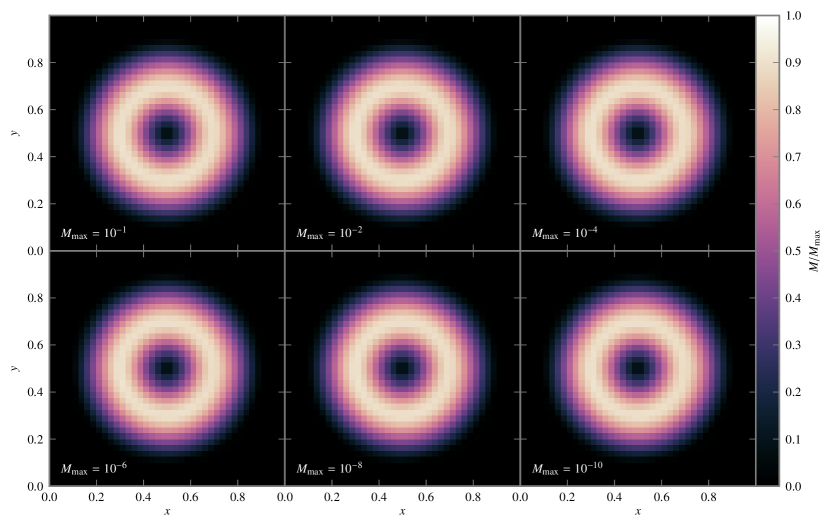
Figure 1: Gresho vortex problem advanced over one full revolution with modified fluxes for different maximum Mach numbers $M_{\mathrm{max}}$ in the setup, as indicated in the plots. Color coded is the Mach number relative to the respective $M_{\mathrm{max}}$.

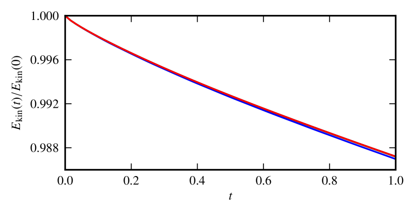
Figure 2: Temporal evolution of the total kinetic energy $E_{\mathrm{kin}}(t)$ relative to its initial value $E_{\mathrm{kin}}(0)$ in the Gresho vortex problem advanced with modified fluxes. The cases for $M_{\mathrm{max}}=10^{-n}$, $n=1,2,3,4,5,6,7,8,9,10$ are overplotted but indistinguishable.

Table 1: Total kinetic energy $E_{\mathrm{kin}}(1.0)$ after one full revolution of the Gresho vortex relative to its initial value $E_{\mathrm{kin}}(0.0)$ for different maximum Mach numbers $M_{\mathrm{max}}$.

$\log M_{\mathrm{max}}$	$E_{\mathrm{kin}}(1.0)/E_{\mathrm{kin}}(0.0)$
$-1$	$0.986974319078$
$-2$	$0.987185681481$
$-3$	$0.987206395072$
$-4$	$0.987208424676$
$-5$	$0.987208767527$
$-6$	$0.987208721327$
$-7$	$0.987208711049$
$-8$	$0.987208711129$
$-9$	$0.987208710852$
$-10$	$0.987208711987$

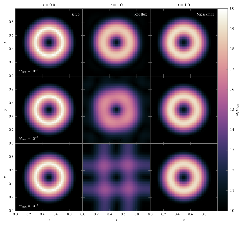
Figure 3: Comparison of the Gresho vortex problem at different initial conditions and computed with different schemes. The rows show the different initial maximum Mach number. The first column is the initial condition, the others show the state after one full rotation using the unmodified Roe solver, and the scheme with the new modifying matrix. Color coded is the Mach number normalized to its initial maximum value.

5 Linear stability of explicit time discretization

5.1 Stability Analysis

The correct reproduction of solutions in the low Mach number limit was achieved by modifying the artificial upwind viscosity matrix – a term that was introduced to stabilize the scheme. This raises the question of the stability of the resulting new method in explicit time discretization.

The investigation of linear stability with the von Neumann method yields results on the time behavior of Fourier modes for a linear(ized) conservation law. If all of the modes are damped in time, the method is called linearly stable. Surely, a necessary requirement is that the method is stable already in one spatial dimension and when integrated in time by a first order method. For simplicity, the following stability analysis is performed with piecewise constant reconstruction, i.e. on a method that is first order in space and time.

Express every quantity $\mathbf{U}^{n}_{i}$ by a Fourier series in space ($\mathbb{i}^{2}=-1$):

$$\mathbf{U}^{n}_{i}=\sum_{k\in\mathbb{Z}}\mathbf{U}^{n}\exp(\mathbb{i}ik\Delta x)$$ (46)

insert this into the fully discrete scheme ($\nu=\frac{\Delta t}{\Delta x}$)

$$\mathbf{U}^{n+1}_{i}=\mathbf{U}^{n}_{i}-\frac{1}{2}\nu\Big{[}A(\mathbf{U}^{n}_{i+1}-\mathbf{U}^{n}_{i-1})-D(\mathbf{U}^{n}_{i+1}-2\mathbf{U}^{n}_{i}+\mathbf{U}^{n}_{i-1})\Big{]}$$ (47)

to obtain, by defining $k\Delta x=:\beta$,

$$\mathbf{U}^{n+1}=\Big{\{}\mathbb{1}-\nu\left[A\mathbb{i}\sin\beta+D(1-\cos\beta)\right]\Big{\}}\mathbf{U}^{n}$$ (48)

The expression in curly brackets is called amplification matrix. Stability of such iterated linear maps needs all its eigenvalues to be less than 1 in absolute value. In particular, it is considered necessary in dellacherie2009a for the absolute value of the acoustic eigenvalues to be strictly less than 1 for the so-called checkerboard-mode $\beta=\pi$. This amounts to non-vanishing eigenvalues of $D$ which is the case for the considered specific choice of $D$, as will be seen later.

Consider the following system

$$\partial_{t}\left(\begin{array}[]{c}q_{1}\\ q_{2}\\ q_{3}\\ \end{array}\right)+\left(\begin{array}[]{ccc}a&a_{12}&0\\ 0&a&a_{23}\\ 0&a_{32}&a\end{array}\right)\partial_{x}\left(\begin{array}[]{c}q_{1}\\ q_{2}\\ q_{3}\\ \end{array}\right)=0$$ (58)

which shall be solved with a time-explicit scheme of Roe-type with a diffusion matrix

$$D=\left(\begin{array}[]{ccc}d_{11}&d_{12}&d_{13}\\ 0&d_{22}&d_{23}\\ 0&d_{32}&d_{33}\end{array}\right)$$ (59)

The Jacobian of hydrodynamics in one spatial dimension and in primitive variables is of this type. As the stability analysis is linear, the equation may be considered in any variables, not necessarily the conserved ones. Moreover, the study of the eigenvalues $\lambda$ of the amplification matrix in (48) equally does not depend on the chosen basis. The property of the diffusion matrix of having just one non-zero entry in the $\varrho$-column will be fulfilled by the one appearing here.

The eigenspace decomposes into

$$1-\nu(a\mathbb{i}\sin\beta+d_{11}(1-\cos\beta))=\lambda$$ (60)

and

$$[1-\nu(a\mathbb{i}\sin\beta+d_{22}(1-\cos\beta))-\lambda][1-\nu(a\mathbb{i}\sin\beta+d_{22}(1-\cos\beta))-\lambda]$$ (61)

$$=\nu^{2}[a_{32}\mathbb{i}\sin\beta+d_{32}(1-\cos\beta)][a_{23}\mathbb{i}\sin\beta+d_{23}(1-\cos\beta)]$$ (62)

Equation (60) is easily recognized as a 1-dimensional stability result. It leads to the stability condition $d_{11}\geq|a|$ and if $d_{11}=|a|$ (as will turn out later in the specific example), then $\nu<\frac{1}{d_{11}}$.

Equation (62) is just the stability condition for the truncated matrices of a reduced system

$$A_{\mathrm{red}}=\left(\begin{array}[]{cc}a&a_{23}\\ a_{32}&a\end{array}\right)\qquad D_{\mathrm{red}}=\left(\begin{array}[]{cc}d_{22}&d_{23}\\ d_{32}&d_{33}\end{array}\right)$$ (63)

Note that the elements $a_{12}$, $d_{12}$ and $d_{13}$ are irrelevant for stability.

Equation (62) can be rewritten as

$$\left(1-\nu\left(a\mathbb{i}\sin\beta+\frac{d_{22}+d_{33}}{2}(1-\cos\beta)\right)-\lambda\right)^{2}=\nu^{2}(\mathcal{A}+\mathcal{B}\mathbb{i})$$ (64)

with

$$\mathcal{A} :=-a_{23}a_{32}\sin^{2}\beta+d_{23}d_{32}(1-\cos\beta)^{2}+\left(\frac{d_{33}-d_{22}}{2}\right)^{2}(1-\cos\beta)^{2}$$ (65)

$$\mathcal{B} :=(a_{23}d_{32}+d_{23}a_{32})(1-\cos\beta)\sin\beta$$ (66)

$$\bar{d} :=\frac{d_{22}+d_{33}}{2}$$ (67)

such that

$$\lambda=1-\nu a\mathbb{i}\sin\beta-\nu\bar{d}(1-\cos\beta)\pm\nu\sqrt{\mathcal{A}+\mathcal{B}\mathbb{i}}$$ (68)

The square root is given by

$$\sqrt{\mathcal{A}+\mathcal{B}\mathbb{i}}=\sqrt{\frac{\sqrt{\mathcal{A}^{2}+\mathcal{B}^{2}}+\mathcal{A}}{2}}+\mathbb{i}\text{\,sgn}(\mathcal{B})\cdot\sqrt{\frac{\sqrt{\mathcal{A}^{2}+\mathcal{B}^{2}}-\mathcal{A}}{2}}$$ (69)

Evaluating $|\lambda|^{2}<1$ leads to

$$\nu<2\frac{\bar{d}(1-\cos\beta)\mp\sqrt{\frac{\sqrt{\mathcal{A}^{2}+\mathcal{B}^{2}}+\mathcal{A}}{2}}}{\left(\bar{d}(1-\cos\beta)\mp\sqrt{\frac{\sqrt{\mathcal{A}^{2}+\mathcal{B}^{2}}+\mathcal{A}}{2}}\right)^{2}+\left(a\sin\beta\mp\text{sgn\,}(\mathcal{B})\sqrt{\frac{\sqrt{\mathcal{A}^{2}+\mathcal{B}^{2}}-\mathcal{A}}{2}}\right)^{2}}$$

The suggested upwinding matrix from miczek2015a is

$$\left(\begin{array}[]{ccc}|v|&\frac{\varrho(-c^{2}\delta+cMv+\delta M^{2}v^{2})}{c\tau}&-\frac{|v|}{c^{2}}+\frac{1}{M\tau}\\ 0&\frac{c^{2}}{M\tau}&\frac{c^{2}\delta+cMv-\delta M^{2}v^{2}}{cM^{2}\varrho\tau}\\ 0&\frac{c\varrho(-c^{2}\delta+cMv+\delta M^{2}v^{2})}{\tau}&\frac{c^{2}}{M\tau}\end{array}\right)$$ (70)

with $\tau=\sqrt{c^{2}(1+\delta^{2})-\delta^{2}M^{2}v^{2}}$.

One can investigate the limit of small $M$. For the components of the upwinding matrix one has (having in mind the two cases $\delta\in\mathcal{O}(\frac{1}{M})$ and $\delta\in\mathcal{O}(1)$):

$$\tau \sim c\sqrt{1+\delta^{2}}$$ (71)

$$\bar{d}\sim\frac{c}{\sqrt{1+\delta^{2}}M}\quad d_{12}\sim\frac{\delta}{\sqrt{1+\delta^{2}}M^{2}}\quad d_{21}\sim-\frac{c^{2}\delta}{\sqrt{1+\delta^{2}}}$$ (72)

Therefore

$$\mathcal{A} =-\frac{c^{2}}{M^{2}}\left(\sin^{2}\beta+\frac{\delta^{2}}{1+\delta^{2}}(1-\cos\beta)^{2}\right)$$ (73)

$$\mathcal{B} =\frac{2cv}{\sqrt{1+\delta^{2}}M}(1-\cos\beta)\sin\beta$$ (74)

where due to a lot of cancellations the exact values were used for $\mathcal{B}$. Whereas in both cases $\mathcal{A}\in\mathcal{O}(1/M^{2})$, one has

$$\mathcal{B} \in\mathcal{O}(1/M)\qquad\text{ if }\delta\in\mathcal{O}(1)$$ (75)

$$\mathcal{B} \in\mathcal{O}(1)\qquad\text{ if }\delta\in\mathcal{O}(1/M)$$ (76)

As, $|\mathcal{A}|=-\mathcal{A}$, $\sqrt{\mathcal{A}^{2}+\mathcal{B}^{2}}-\mathcal{A}\sim 2|\mathcal{A}|$ and

$$\sqrt{\mathcal{A}^{2}+\mathcal{B}^{2}}+\mathcal{A}\sim|\mathcal{A}|\frac{\mathcal{B}^{2}}{2\mathcal{A}^{2}}=\frac{\mathcal{B}^{2}}{2|\mathcal{A}|}\in\begin{cases}\mathcal{O}(1)&\text{ if }\delta\in\mathcal{O}(1)\\ \mathcal{O}(M^{2})&\text{ if }\delta\in\mathcal{O}(1/M)\end{cases}$$ (77)

The term $\sqrt{\frac{\sqrt{\mathcal{A}^{2}+\mathcal{B}^{2}}+\mathcal{A}}{2}}$ will be compared to

$$\bar{d}(1-\cos\beta)\in\begin{cases}\mathcal{O}(1/M)&\text{ if }\delta\in\mathcal{O}(1)\\ \mathcal{O}(1)&\text{ if }\delta\in\mathcal{O}(1/M)\end{cases}$$ (78)

and the latter wins in both cases. Therefore

$$\nu <2\frac{d(1-\cos\beta)}{d^{2}(1-\cos\beta)^{2}+\left(c\sin\beta\mp\text{sgn\,}(B)\sqrt{|A|}\right)^{2}}$$ (79)

$$\sim 2\frac{\frac{c}{\sqrt{1+\delta^{2}}M}(1-\cos\beta)}{\frac{c^{2}}{(1+\delta^{2})M^{2}}(1-\cos\beta)^{2}+\frac{c^{2}}{M^{2}}\left|\sin^{2}\beta-\frac{\delta^{2}}{1+\delta^{2}}(1-\cos\beta)^{2}\right|}$$ (80)

$$=\frac{M}{c}\frac{\frac{2}{\sqrt{1+\delta^{2}}}}{\frac{1}{1+\delta^{2}}(1-\cos\beta)+\left|(1+\cos\beta)-\frac{\delta^{2}}{1+\delta^{2}}(1-\cos\beta)\right|}$$ (81)

$$=\frac{M}{c}\frac{2\sqrt{1+\delta^{2}}}{1-\cos\beta+\left|1+(1+2\delta^{2})\cos\beta\right|}$$ (82)

Now a minimum over all $\beta\in[0,2\pi)$ has to be performed in order to obtain the global maximum value of $\nu$. If $\delta\in\mathcal{O}(1)$ (in particular one might be interested to recover for $\delta=0$ the usual Roe scheme) then

$$\nu_{\text{max}}\sim\frac{M}{c}$$ (83)

if a suitable minimizing $\cos\beta_{\text{min}}$ exists, which is $\mathcal{O}(1)$ (trivially the case for $\delta=0$).

However if $\delta\in\mathcal{O}(1/M)$, then $|\cos\beta_{\text{min}}|=1$ and

$$\nu_{\text{max}} \sim\frac{M}{c}\frac{\sqrt{1+\delta^{2}}}{\delta^{2}}\in\mathcal{O}\left(\frac{M^{2}}{c}\right)$$ (84)

5.2 Numerical Verification

This more restrictive CFL condition is also observed in the experiments. As a test setup for CFL stability we use a one-dimensional sound wave. The initial profile is given by

$$\varrho(x) =p_{0}(1+M\cos(kx)),$$ (85)

$$u(x) =Mc_{0}\cos(kx),$$ (86)

$$p(x) =p_{0}+\varrho_{0}c_{0}^{2}M\cos(kx),$$ (87)

with free parameters for background pressure $p_{0}$, density $\varrho_{0}$, and the corresponding speed of sound $c_{0}=\sqrt{\gamma p_{0}/\varrho_{0}}$. The amplitude and thus the Mach number of this sound wave can be adjusted with the parameter $M$. The size of the domain is $[0,1)$ with periodic boundary conditions. We run this setup for a time $t=1$ with explicit forward Euler time-stepping and constant reconstruction. Explicit integration in time is very inefficient at low Mach numbers and it can take many million time steps for the instability to become obvious (i.e. visible noise in the velocity field, negative densities, …). To facilitate the analysis we compare the growth of the high-frequency Fourier modes, for which we expect exponential growth in the unstable case. We use

$$\sum_{i=N/2}^{N}|\hat{u}_{i}|,$$ (88)

where $\hat{u}$ is the discrete Fourier transform of $u(x)$ and $N$ is the number of grid points. We test the growth of this quantity for a range of $M$ and some values of $\Delta t$ above and below the critical CFL time step, both for the usual, and the modified Roe scheme. To emphasize the effect of the numerical flux, we intentionally choose forward Euler time stepping and constant reconstruction of the interface values. The results of this experiment at $M=10^{-3}$ are summarized in Fig. 4. The tests using the standard Roe scheme confirm that the stability threshold is at CFL 1, as expected. For the Roe–Miczek scheme we need an additional factor of $M$ in the time step criterion as it was shown above. The Roe–Turkel scheme was not stable for any of the tested time steps.

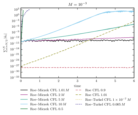
Figure 4: Stability tests of a sound wave at Mach number $M=10^{-3}$ using constant reconstruction and forward Euler time stepping. The line styles signify the different numerical fluxes. For the Roe–Miczek and Roe–Turkel scheme the CFL condition was multiplied by $M$ for most tests as indicated.

The stability of the discretization of (1)–(3) for the particular case of checkerboard modes ($\beta=\pi$) has equally been confirmed by experiments.

6 Implicit time discretization

In the light of the stricter CFL condition of some of the low Mach schemes mentioned above, it is natural to turn to implicit time discretizations to allow larger time steps. Even for time-explicit schemes with the standard CFL condition time steps become prohibitively small: they scale with the inverse of the sound speed and therefore are bound to the acoustic time scale, i.e. the sound-crossing time in one computational grid cell. In contrast, the criterion for selecting the time step in implicit schemes is not derived from considerations of stability of the scheme but rather from the intended accuracy of the solution. In the low Mach case one is usually interested in phenomena that are associated with the fluid flow instead of sound waves. In order to accurately resolve the flow, the time step should be restricted to the flow crossing time over a grid cell – the advective time step criterion. The ratio between the acoustic and the advective time steps (and thus the ratio of time steps to be taken for bridging the same physical time interval) is a function of the Mach number. Even considering the increased computational cost of implicit time steps, it is expected that there is a certain Mach number below which an implicit scheme is more efficient than explicit time discretization. But the threshold (and the very feasibility of an implicit time integration) depends on the system of equations to be solved and on the efficiency of the solution method.

Implicit time stepping for the Euler equations involves the solution of a large nonlinear system of equations. In the three-dimensional case the number of equations is $5N_{x}N_{y}N_{z}$, where is $N_{x,y,z}$ is the number of grid cells in $x$, $y$, or $z$ direction. Even for a moderately sized problem of $512^{3}$ cells this already yields about $6.7\times 10^{8}$ nonlinear coupled equations with the same number of unknowns. We use the Newton–Raphson method for the solution, which itself requires the solution of a large linear system of equations given by the Jacobian of the nonlinear one. Apart from the particular implementation approach, the success and efficiency of the scheme critically depend on the structure of the system of equations to be solved. In particular, a high condition number of this system would severely impede the ability to find solutions efficiently. The particular definition of the condition number $\kappa$, that we use here, is,

$$\kappa=\|A\|_{1}\cdot\|A^{-1}\|_{1},$$ (89)

where $A$ is the Jacobian matrix of the nonlinear system. We use the 1-norm as is it computationally less expensive to evaluate compared to the 2-norm but still has similar significance for the solution efficiency of the linear system.

In Fig. 5 we show the effects on the condition number for the different modified diffusion matrices presented in this article. In order to get a representative condition number for different discretizations under realistic conditions we pick a turbulent flow field that was produced using stochastic forcing eswaran1988a ; schmidt2006e . The first obvious feature of the curves is that they are almost identical in the high and low Mach number limit. In the regime $M\lesssim 10^{-6}$ this is due to the dominating influence of the central flux terms, which all the other schemes also include. In the Mach number regime from about $10^{-4}$ to $10^{-2}$ the condition number of the Roe-type schemes is almost Mach number independent, with the condition number of the Roe–Turkel scheme being significantly higher than the other two. For practical applications using implicit time stepping this means that the Roe–Miczek scheme is as efficient as the standard Roe scheme while still giving an accurate result like the Roe–Turkel scheme. Moreover it has been demonstrated hammer2015a that the corresponding implementation scales up to $\sim$100,000 cores making it suitable for highly resolved simulations.

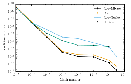
Figure 5: Mach number dependence of the condition number of the unpreconditioned Jacobian matrix that occurs in the solution of the nonlinear system. It was obtained on a $16^{3}$ grid in the simulation of stochastically driven turbulence.

7 Application to unsteady low Mach number flows

The application examples demonstrated thus far are steady state problems. The fact that a scheme behaves well at low Mach numbers for these problems might not be representative of good low Mach behavior in general. Because of this we apply the Roe–Miczek scheme to a number of unsteady flow problems at low Mach numbers.

The Taylor–Green vortex (TGV) taylor1937a is a large-scale, three-dimensional vortex that decays to smaller vortices, thereby creating a turbulent flow pattern. Its advantages are that it can be easily implemented by just setting an initial condition and it provides a simple estimate for the Reynolds number. In the context of the Euler equations we can use it to measure numerical viscosity.

We use the initial conditions given in drikakis2007a ,

$$\varrho(t=0) =\varrho_{0}=1.178\times 10^{-3},$$ (90)

$$u(t=0) =u_{0}\sin(kx)\cos(ky)\cos(kz),$$

$$v(t=0) =-u_{0}\cos(kx)\sin(ky)\cos(kz),$$

$$w(t=0) =0,$$

$$u_{0} =10^{4},$$

$$k =10^{-2}$$

$$p(t=0) =p_{0}+\left[{u_{0}}^{2}\varrho/16\right]\left[2+\cos\frac{2z}{100}\right]\left[\cos\frac{2x}{100}+\cos\frac{2y}{100}\right],$$

$$p_{0} =10^{6}.$$

For comparability with other results in the literature we choose the value $\gamma=1.4$ in the equation of state (Eq. (95)). The maximum Mach number of this setup is $M_{\text{max}}=u_{0}/\sqrt{\gamma p_{0}/\varrho_{0}}\approx 0.29$. We can easily scale this setup to lower Mach numbers by multiplying $u_{0}$ with the appropriate factor.

To be able to compare simulations at different Mach numbers, we scale certain quantities (denoted by ^∗). The relations are

$$t^{*}=ku_{0}t,\quad K^{*}=K/{u_{0}}^{2},\quad\Omega^{*}=\Omega/(ku_{0})^{2}.$$ (91)

To test the effect of the diffusion matrix modification we calculate the numerical Reynolds number of the usual Roe scheme and the modified one at different resolutions and Mach numbers. The Reynolds number is purely numerical as we do not include any explicit viscosity terms. We use the expression given in taylor1937a ,

$$\frac{dK^{*}}{dt^{*}}=-\frac{\Omega^{*}}{\text{Re}},$$ (92)

with the mean of kinetic energy $K$ and the mean enstrophy $\Omega$,

$$K=\frac{1}{2}\langle|\mathbf{v}|^{2}\rangle,\quad\Omega=\frac{1}{2}\langle|\nabla\times\mathbf{v}|^{2}\rangle.$$ (93)

The operation $\langle\cdot\rangle$ is a volumetric average. Both quantities can be independently computed from the velocity field $\mathbf{v}$.

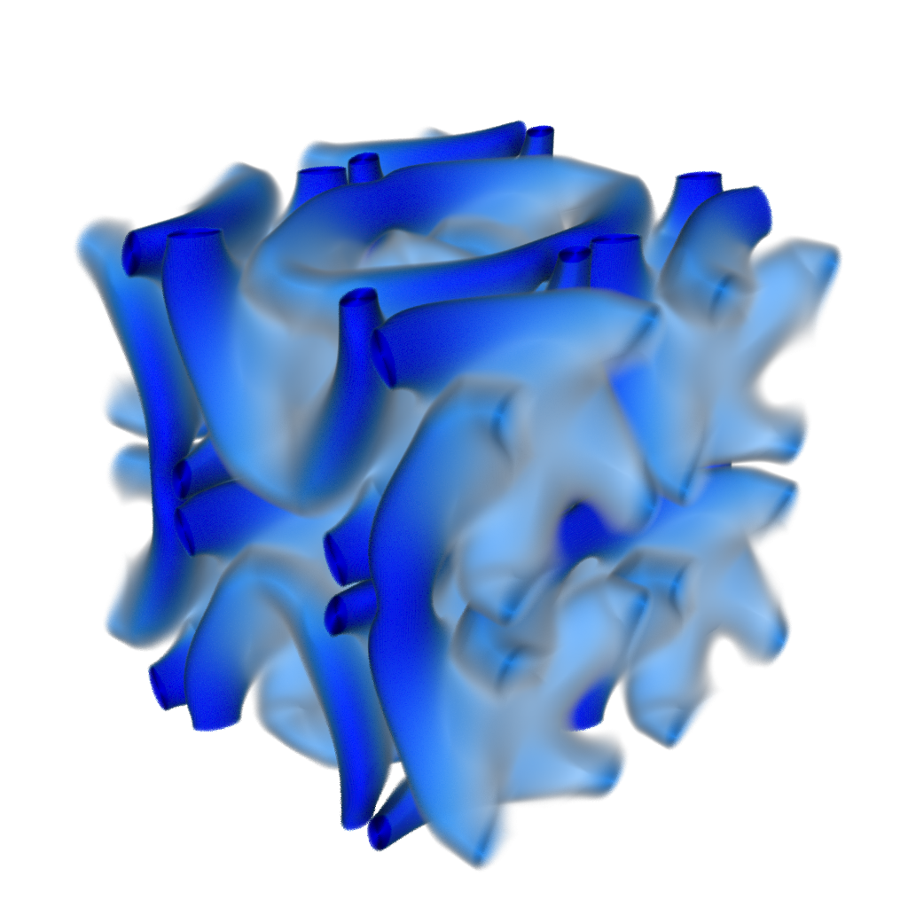
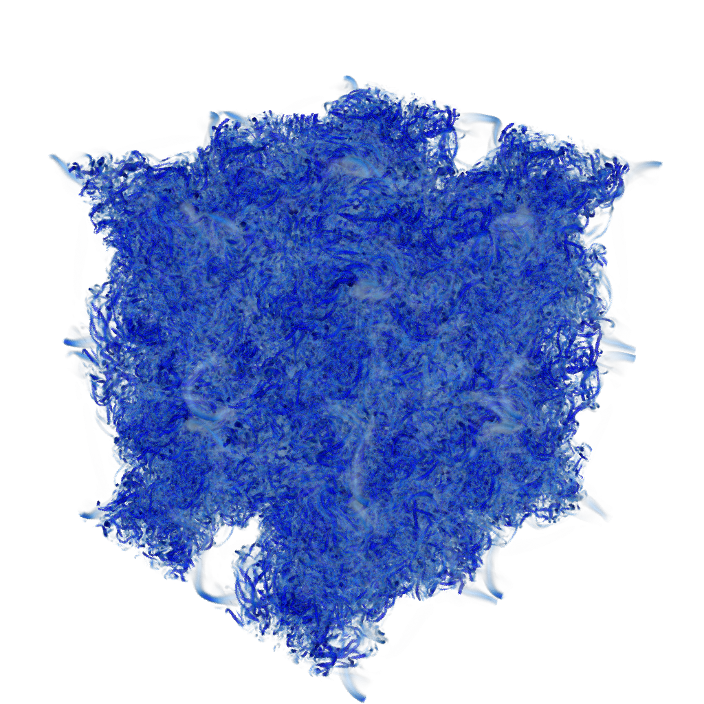
$t^{*}={0}$	$t^{*}={0.96}$	$t^{*}={3.05}$
scale $10$	scale $10$	scale $1000$
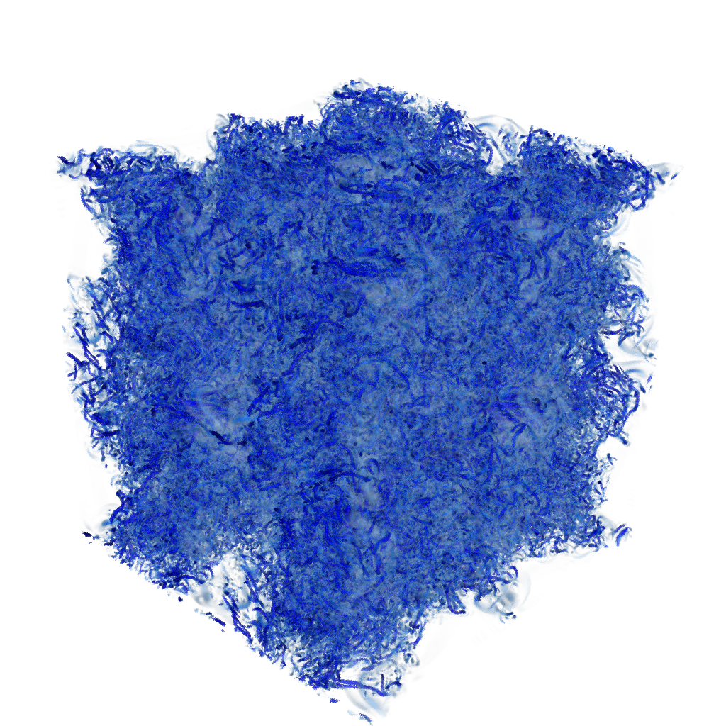
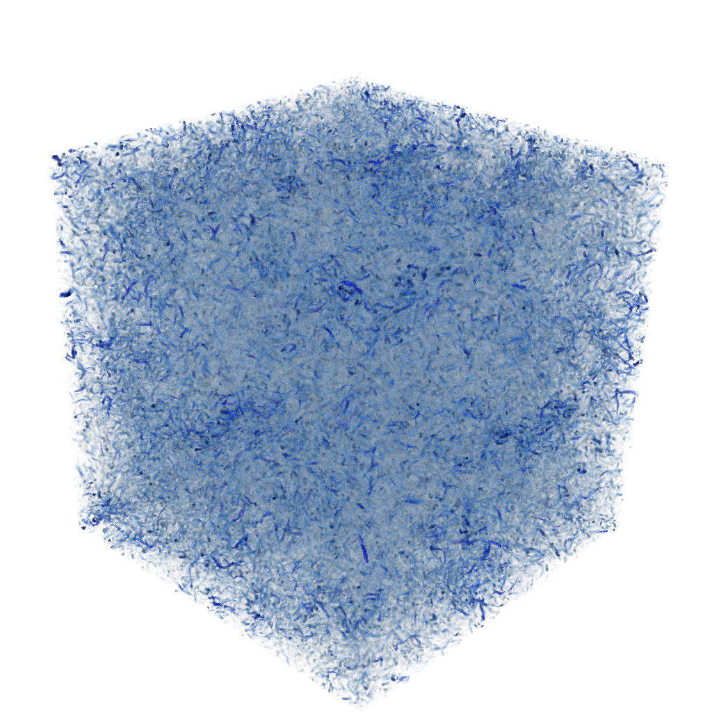
$t^{*}={3.34}$	$t^{*}={5.01}$	$t^{*}={8.70}$
scale 1000	scale 1000	scale 250

Figure 6: Temporal evolution of vortex cores in the Taylor–Green vortex visualized using a criterion from jeong1995a . The Mach number of the initial configuration was set to $10^{-2}$. The simulation was run at a resolution of $512^{3}$ grid cells using the Roe–Miczek scheme and implicit ESDIRK34 time stepping. The magnitude of the color scale was adjusted as stated below each panel.

Figure 6 visualizes the decay of the large scale vortices to smaller scales and their eventual dissipation using a criterion from jeong1995a .

The test in Fig. 7 shows kinetic energy dissipation rate of the vortex at different Mach numbers computed with a fixed grid size of $128^{3}$ cells. It is expected that this rate is independent of Mach number in the nondimensional variables of Eq. (91). This is very well fulfilled for the modified Roe scheme from miczek2015a but not for the original Roe scheme.

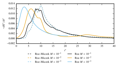
Figure 7: Taylor–Green vortex simulated at a fixed resolution of $128^{3}$ grid cells. The solid lines were computed using the Roe flux, the dashed lines using the modified flux miczek2015a . The colors signify different initial Mach numbers.

8 Tests in the High-Mach number regime

To qualify as a scheme for all Mach numbers it has to be ensured that it behaves correctly in the presence of shocks. The modifying matrix, Eq. (31), continuously approaches the identity matrix as the Mach number increases to 1. The newly proposed scheme is identical to the original Roe scheme for $M_{\text{loc}}\geq 1$. The Roe scheme, however, is known to violate the entropy condition in transonic rarefactions, which is cured by introducing an entropy fix (see pelanti2001a for an overview). Here we test if this treatment interferes with our low Mach number modifications. For the present study we chose to implement the fix suggested by harten1983b . We use a shock tube with isentropic initial conditions, which makes the entropy problem and its solution obvious. The initial setup in primitive variables is

$$(\varrho,u,p)(x,0)=\begin{cases}(3,0.9,3)&\text{for $x<0.5$},\\ (1,0.9,3^{1-\gamma})&\text{otherwise}.\end{cases}$$ (94)

The value $\gamma$ is the adiabatic index in the ideal gas equation of state (95), i.e. the internal energy is $e=p/(\gamma-1)$. Figure 8 shows the solution at time $t=0.2$ for the Roe–Miczek scheme with and without the entropy fix. Implementing an entropy fix shows no interference with the introduced modifications.

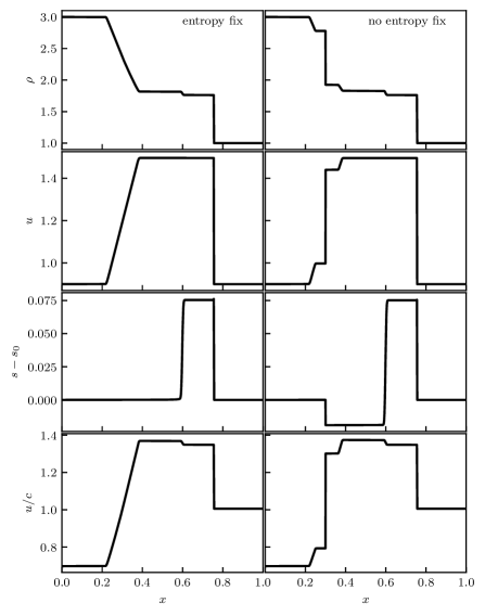
Figure 8: This shows density (top row), velocity (second row), deviation of entropy from its initial value (third row), and Mach number (bottom row) of a transonic shock tube defined by the initial conditions in Eq. (94) at time $t=0.2$. The right column was computed using the Roe–Miczek scheme without any entropy fix. The left column used the same scheme with the entropy fix suggested in harten1983b .

9 Conclusions

We have presented a finite volume solver for the compressible Euler equations (miczek2015a ) with the following properties:

1. it is preserving the asymptotics of the low Mach limit

2. it ensures the kinetic energy of the flow is not excessively dissipated by the numerics near the incompressible regime

3. it is a linearly stable scheme

4. the inversion of the large system of equations arising from implicit time discretization has a good condition number.

Requirement (ii) reflects well the issue of growing numerical diffusion in the low Mach limit observed for shock-capturing schemes, and might be easier to check than (i).

We have shown numerical simulations with this scheme that work for Mach numbers as low as $10^{-10}$. The method can also be applied to flows with high Mach number, where it continuously approaches the Roe solver. For transonic flows our modification does not interfere with the entropy fix. In this sense the method of Miczek et al. miczek2015a constitutes an all-Mach number scheme.

We conclude that when devising a low Mach number scheme for the Euler equations it is important that the discrete equations reflect the nature of the limit system for finite discretizations already. It thus is not sufficient to ensure that asymptotically the discrete equations become consistent discretizations of the limit system. We show that in addition one needs to satisfy the requirements ii, iii, iv for such a scheme to be feasible in practice.

In upcoming work we plan to extend these properties to the Euler equations with a gravitational source term, where one needs to ensure in addition that the scheme is well-balanced.

Appendix

The limit of low Mach numbers in the context of the Euler equations (1)–(3) is best explored by introducing a family of solutions, parametrized by a real dimensionless number $M>0$, $M\to 0$. Writing $f\in\mathcal{O}(M^{p})$ means that the leading order of the expansion of $f$ in powers of $M$ is $M^{p}$, i.e. $f=M^{p}(f^{(0)}+f^{(1)}M+\ldots)$, with the functions $f^{(i)}$ not depending on $M$.
Only two requirements are needed to derive the rescaled Euler equations:

• The local Mach number $\displaystyle M_{\text{loc}}(\mathbf{x},t):=|\mathbf{v}(\mathbf{x},t)|/\sqrt{\frac{\gamma p(\mathbf{x},t)}{\varrho(\mathbf{x},t)}}$ shall be scaling uniformly with $M$ as $M\to 0$: $M_{\text{loc}}\in\mathcal{O}(M)$.

• Every member of the family shall fulfill the same equation of state

  $$E=\frac{p}{\gamma-1}+\frac{1}{2}\varrho|\mathbf{v}|^{2}.$$ (95)

The most general asymptotic scalings in this case are

$$\mathbf{x} =M^{\mathfrak{a}}\tilde{\mathbf{x}}, t =M^{\mathfrak{b}}\tilde{t},$$ (96)

$$\varrho(\mathbf{x},t) =M^{\mathfrak{c}+2-2\mathfrak{d}}\tilde{\varrho}(\mathbf{\tilde{x}},\tilde{t}), \mathbf{v}(\mathbf{x},t) =M^{\mathfrak{d}}\tilde{\mathbf{v}}(\mathbf{\tilde{x}},\tilde{t}),$$ (97)

$$E(\mathbf{x},t) =M^{\mathfrak{c}}\tilde{E}(\mathbf{\tilde{x}},\tilde{t}), p(\mathbf{x},t) =M^{\mathfrak{c}}\tilde{p}(\mathbf{\tilde{x}},\tilde{t}),$$ (98)

with $\mathfrak{a,b,c,d}$ arbitrary numbers, as can be found from a direct computation. It is understood that quantities with a tilde are $\mathcal{O}(1)$ when expanded as power series in $M$. An example of such a family of solutions is given by the Gresho vortex setup in (44)–(45).

Furthermore every member of the family shall fulfill the Euler equations. Inserting the above scalings yields a system of equations that is fulfilled by quantities with a tilde. These equations shall be called rescaled, and cannot be the Euler equations again, because the Mach number changes. They are found to be

$$\tilde{E}=\frac{\tilde{p}}{\gamma-1}+\frac{1}{2}M^{2}\tilde{\varrho}|\tilde{\mathbf{v}}|^{2}$$ (99)

and

$$M^{\mathfrak{a}-\mathfrak{d}-\mathfrak{b}}\partial_{t}\tilde{\varrho}+\nabla\cdot(\tilde{\varrho}\tilde{\mathbf{v}})=0,$$ (100)

$$M^{\mathfrak{a}-\mathfrak{d}-\mathfrak{b}}\partial_{t}(\tilde{\varrho}\tilde{\mathbf{v}})+\nabla\cdot\left(\tilde{\varrho}\tilde{\mathbf{v}}\otimes\tilde{\mathbf{v}}+\frac{\tilde{p}}{M^{2}}\cdot\mathbb{1}\right)=0,$$ (101)

$$M^{\mathfrak{a}-\mathfrak{d}-\mathfrak{b}}\partial_{t}\tilde{E}+\nabla\cdot(\tilde{\mathbf{v}}(\tilde{E}+\tilde{p}))=0.$$ (102)

Observe the fact that the kinetic energy obtains an additional factor of $M^{2}$ in the equation of state.

The factor in front of the time derivatives is related to the dimensionless Strouhal number

$$\text{{Str}}_{\text{loc}} =\frac{x}{|\mathbf{v}|t}=\frac{M^{\mathfrak{a}}\tilde{x}}{M^{\mathfrak{d}}\tilde{\mathbf{v}}\cdot M^{\mathfrak{b}}\tilde{t}}.$$ (103)

This factor is not identical to the Strouhal number, but is just its asymptotic $M$-scaling. As an additional condition on the family of solutions one is tempted to insist on $\text{{Str}}\in\mathcal{O}(1)$, i.e. $\mathfrak{a}-\mathfrak{d}-\mathfrak{b}=0$. This corresponds to adapting the time scales to the speed of the fluid (and not to sound wave crossing times).
Different ways of decreasing the Mach number (e.g. by decreasing the value of the velocity, or increasing the sound speed instead, or a combination of both) are equivalent and should result in the same rescaled equations. This explains why the precise value of $\mathfrak{a,b,c,d}$ does not matter for the form of the rescaled equations. Only these equations will be considered in what follows and we drop the tilde.

- (1) Asano, K.: On the incompressible limit of the compressible euler equation. Japan Journal of Applied Mathematics 4(3), 455–488 (1987)
- (2) Chalons, C., Girardin, M., Kokh, S.: An All-Regime Lagrange-Projection Like Scheme for the Gas Dynamics Equations on Unstructured Meshes. Communications in Computational Physics 20, 188–233 (2016). DOI 10.4208/cicp.260614.061115a
- (3) Cordier, F., Degond, P., Kumbaro, A.: An Asymptotic-Preserving all-speed scheme for the Euler and Navier-Stokes equations. Journal of Computational Physics 231, 5685–5704 (2012). DOI 10.1016/j.jcp.2012.04.025
- (4) Degond, P., Tang, M.: All speed method for the euler equation in the low mach number limit. Communications in Computational Physics 10, 1–31 (2011)
- (5) Dellacherie, S.: Checkerboard modes and wave equation. In: Proceedings of ALGORITMY, vol. 2009, pp. 71–80 (2009)
- (6) Dellacherie, S.: Analysis of godunov type schemes applied to the compressible euler system at low mach number. Journal of Computational Physics 229(4), 978–1016 (2010). DOI 10.1016/j.jcp.2009.09.044. URL http://www.sciencedirect.com/science/article/pii/S0021999109005361
- (7) Drikakis, D., Fureby, C., Grinstein, F.F., Youngs, D.: Simulation of transition and turbulence decay in the taylor–green vortex. Journal of Turbulence 8, N20 (2007). DOI 10.1080/14685240701250289. URL http://www.tandfonline.com/doi/abs/10.1080/14685240701250289
- (8) Ebin, D.G.: The motion of slightly compressible fluids viewed as a motion with strong constraining force. Annals of mathematics pp. 141–200 (1977)
- (9) Eswaran, V., Pope, S.B.: An examination of forcing in direct numerical simulations of turbulence. Computers and Fluids 16, 257–278 (1988)
- (10) Gresho, P.M., Chan, S.T.: On the theory of semi-implicit projection methods for viscous incompressible flow and its implementation via a finite element method that also introduces a nearly consistent mass matrix. part 2: Implementation. International Journal for Numerical Methods in Fluids 11(5), 621–659 (1990). DOI 10.1002/fld.1650110510. URL http://dx.doi.org/10.1002/fld.1650110510
- (11) Guillard, H., Murrone, A.: On the behavior of upwind schemes in the low mach number limit: Ii godunov type schemes. Computers & Fluids 33, 655–675 (2004)
- (12) Guillard, H., Viozat, C.: On the behaviour of upwind schemes in the low mach number limit. Computers & Fluids 28(1), 63 – 86 (1999). DOI 10.1016/S0045-7930(98)00017-6. URL http://www.sciencedirect.com/science/article/pii/S0045793098000176
- (13) Haack, J., Jin, S., Liu, J.G.: An All-Speed Asymptotic-Preserving Method for the Isentropic Euler and Navier-Stokes Equations. Communications in Computational Physics 12, 955–980 (2012). DOI 10.4208/cicp.250910.131011a
- (14) Hammer, N., Jamitzky, F., Satzger, H., Allalen, M., Block, A., Karmakar, A., Brehm, M., Bader, R., Iapichino, L., Ragagnin, A., Karakasis, V., Kranzlmüller, D., Bode, A., Huber, H., Kühn, M., Machado, R., Grünewald, D., Edelmann, P.V.F., Röpke, F.K., Wittmann, M., Zeiser, T., Wellein, G., Mathias, G., Schwörer, M., Lorenzen, K., Federrath, C., Klessen, R., Bamberg, K., Ruhl, H., Schornbaum, F., Bauer, M., Nikhil, A., Qi, J., Klimach, H., Stüben, H., Deshmukh, A., Falkenstein, T., Dolag, K., Petkova, M.: Extreme scale-out supermuc phase 2 - lessons learned. In: G.R. Joubert, H. Leather, M. Parsons, F.J. Peters, M. Sawyer (eds.) Parallel Computing: On the Road to Exascale, Proceedings of the International Conference on Parallel Computing, ParCo 2015, 1-4 September 2015, Edinburgh, Scotland, UK, Advances in Parallel Computing, vol. 27, pp. 827–836. IOS Press (2015). DOI 10.3233/978-1-61499-621-7-827. URL http://dx.doi.org/10.3233/978-1-61499-621-7-827
- (15) Harten, A., Hyman, J.M.: Self-Adjusting Grid Methods for One-Dimensional Hyperbolic Conservation Laws. Journal of Computational Physics 50, 235–269 (1983). DOI 10.1016/0021-9991(83)90066-9
- (16) Isozaki, H.: Wave operators and the incompressible limit of the compressible euler equation. Communications in mathematical physics 110(3), 519–524 (1987)
- (17) Jeong, J., Hussain, F.: On the identification of a vortex. Journal of Fluid Mechanics 285, 69–94 (1995). DOI 10.1017/S0022112095000462
- (18) Klainerman, S., Majda, A.: Singular limits of quasilinear hyperbolic systems with large parameters and the incompressible limit of compressible fluids. Communications on pure and applied Mathematics 34(4), 481–524 (1981)
- (19) Klein, R.: Semi-implicit extension of a godunov-type scheme based on low mach number asymptotics I: One-dimensional flow. Journal of Computational Physics 121, 213–237 (1995). DOI 10.1016/S0021-9991(95)90034-9
- (20) Kreiss, H.O., Lorenz, J., Naughton, M.: Convergence of the solutions of the compressible to the solutions of the incompressible navier-stokes equations. Advances in Applied Mathematics 12(2), 187–214 (1991)
- (21) Métivier, G., Schochet, S.: The incompressible limit of the non-isentropic euler equations. Archive for rational mechanics and analysis 158(1), 61–90 (2001)
- (22) Miczek, F., Röpke, F.K., Edelmann, P.V.F.: New numerical solver for flows at various mach numbers. Astronomy & Astrophysics 576, A50 (2015). DOI 10.1051/0004-6361/201425059
- (23) Oßwald, K., Siegmund, A., Birken, P., Hannemann, V., Meister, A.: L2roe: a low dissipation version of roe’s approximate riemann solver for low mach numbers. International Journal for Numerical Methods in Fluids (2015). DOI 10.1002/fld.4175. URL http://dx.doi.org/10.1002/fld.4175. Fld.4175
- (24) Pelanti, M., Quartapelle, L., Vigevano, L.: A review of entropy fixes as applied to roe’s linearization. Teaching material of the Aerospace and Aeronautics Department of Politecnico di Milano (2001)
- (25) Rieper, F.: A low-mach number fix for roe’s approximate riemann solver. Journal of Computational Physics 230(13), 5263–5287 (2011)
- (26) Roe, P.L.: Approximate riemann solvers, parameter vectors, and difference schemes. Journal of Computational Physics 43(2), 357 – 372 (1981). DOI 10.1016/0021-9991(81)90128-5
- (27) Schmidt, W., Hillebrandt, W., Niemeyer, J.C.: Numerical dissipation and the bottleneck effect in simulations of compressible isotropic turbulence. Comp. Fluids. 35, 353–371 (2006). DOI doi:10.1016/j.compfluid.2005.03.002
- (28) Schochet, S.: Fast singular limits of hyperbolic pdes. Journal of Differential Equations 114(2), 476–512 (1994). DOI 10.1006/jdeq.1994.1157. URL http://www.sciencedirect.com/science/article/pii/S0022039684711570
- (29) Stephan, M., Docter, J.: Juqueen: Ibm blue gene/q® supercomputer system at the jülich supercomputing centre. Journal of large-scale research facilities JLSRF 1, A1 (2015). DOI 10.17815/jlsrf-1-18. URL http://dx.doi.org/10.17815/jlsrf-1-18
- (30) Taylor, G.I., Green, A.E.: Mechanism of the Production of Small Eddies from Large Ones. Royal Society of London Proceedings Series A 158, 499–521 (1937). DOI 10.1098/rspa.1937.0036
- (31) Toro, E.F.: Riemann Solvers and Numerical Methods for Fluid Dynamics: A Practical Introduction. Springer, Berlin Heidelberg (2009). URL http://books.google.de/books?id=SqEjX0um8o0C
- (32) Turkel, E.: Preconditioning Techniques in Computational Fluid Dynamics. Annual Review of Fluid Mechanics 31, 385–416 (1999). DOI 10.1146/annurev.fluid.31.1.385
- (33) Ukai, S., et al.: The incompressible limit and the initial layer of the compressible euler equation. Journal of Mathematics of Kyoto University 26(2), 323–331 (1986)
- (34) van Leer, B.: Towards the ultimate conservative difference scheme. V – A second-order sequel to godunov’s method. Journal of Computational Physics 32, 101–136 (1979). DOI 10.1016/0021-9991(79)90145-1
- (35) Weiss, J.M., Smith, W.A.: Preconditioning applied to variable and constant density flows. AIAA Journal 33, 2050–2057 (1995). DOI 10.2514/3.12946