Hall-effect Mediated Magnetic Flux Transport in Protoplanetary Disks

Abstract

The global evolution of protoplanetary disks (PPDs) has recently been shown to be largely controlled by the amount of poloidal magnetic flux threading the disk. The amount of magnetic flux must also co-evolve with the disk, as a result of magnetic flux transport, a process which is poorly understood. In weakly ionized gas as in PPDs, magnetic flux is largely frozen in the electron fluid, except when resistivity is large. When the disk is largely laminar, we show that the relative drift between the electrons and ions (the Hall-drift), and the ions and neutral fluids (ambipolar-drift) can play a dominant role on the transport of magnetic flux. Using two-dimensional simulations that incorporate the Hall effect and ambipolar diffusion (AD) with prescribed diffusivities, we show that when large-scale poloidal field is aligned with disk rotation, the Hall effect rapidly drags magnetic flux inward at the midplane region, while it slowly pushes flux outward above/below the midplane. This leads to a highly radially elongated field configuration as a global manifestation of the Hall-shear instability. This field configuration further promotes rapid outward flux transport by AD at the midplane, leading to instability saturation. In quasi-steady state, magnetic flux is transported outward at approximately the same rate at all heights, and the rate is comparable to the Hall-free case. For anti-aligned field polarity, the Hall effect consistently transports magnetic flux outward, leading to a largely vertical field configuration in the midplane region. The field lines in the upper layer first bend radially inward and then outward to launch a disk wind. Overall, the net rate of outward flux transport is about twice faster than the aligned case. In addition, the rate of flux transport increases with increasing disk magnetization. The absolute rate of transport is sensitive to disk microphysics which remains to be explored in future studies.

1. Introduction

Global structure and evolution of protoplanetary disks (PPDs) play a fundamental role in almost all stages of planet formation. It has recently been realized that due to the weakly ionized nature of PPD gas, the magnetorotational instability (MRI, Balbus & Hawley, 1991) is almost entirely suppressed in the inner region of PPDs (Bai & Stone, 2013b; Bai, 2013; Gressel et al., 2015), and is substantially damped in the outer disk (Simon et al., 2013a; Bai, 2015). Efficient angular momentum transport requires the disk to be threaded with external large-scale poloidal magnetic flux, presumably inherited from the star formation process, and a magnetized disk wind is likely the primary mechanism to drive disk accretion. Because the wind kinematics strongly depends on disk magnetization (e.g., Bai et al., 2016), global disk evolution is primarily governed by the amount of poloidal magnetic flux threading the disks, and its radial distribution (Bai, 2016). Before we can fully understand global disk evolution, a more fundamental question is, what determines the amount and distribution of magnetic flux threading PPDs? Equivalently, how is magnetic flux transported in PPDs?

Magnetic flux transport has conventionally been modeled as a competition between inward advection by viscously-driven accretion, and outward diffusion by (turbulent or physical) resistivity (Lubow et al., 1994). While more recent works have taken into account disk vertical structure (Rothstein & Lovelace, 2008; Guilet & Ogilvie, 2012, 2013), or radial resistivity profile (Okuzumi et al., 2014; Takeuchi & Okuzumi, 2014), they all fall into the same advection-diffusion framework, which ignores the wind-driven accretion process, and detailed disk microphysics.

Weakly ionized PPDs are subject to three non-ideal magnetohydrodynamic (MHD) effects, namely, Ohmic resistivity, the Hall effect, and ambipolar diffusion (AD). To our knowledge, the Hall effect and AD have not been considered in the theory of magnetic flux transport in accretion disks. The problem of magnetic flux transport is directly coupled to the gas dynamics, and current studies in PPDs have mostly focused on the gas dynamics itself.

Unlike resistivity, which diffuses magnetic field isotropically, both AD and the Hall effect are anisotropic. AD shares some similarities with Ohmic resistivity that acts to diffuse magnetic flux outwards for typical field configurations, its anisotropic nature also introduces novel ingredients, as we will address in this paper. The Hall effect behaves completely differently, which we will focus on in this work. It is well known that the Hall term affects the disk dynamics in polarity-dependent ways (Wardle, 1999; Wardle & Salmeron, 2012). Local semi-analytical wind solutions that include these effects have been studied in the literature (e.g., Wardle & Koenigl, 1993; Königl et al., 2010; Salmeron et al., 2011). Local shearing-box simulations with imposed constant net vertical field have also found very different behaviors for different field polarities (Sano & Stone, 2002a, b; Kunz & Lesur, 2013; Bai, 2014, 2015; Simon et al., 2015). Evidence for rapid and polarity-dependent magnetic flux transport has been reported (Bai, 2014). However, being local solutions/simulations, the results depend on the imposed boundary conditions. Consequently, the rate of magnetic flux transport can not be reliably determined, and in some semi-analytical solutions, it is in fact imposed as a free parameter.

In this paper, we first point out in Section 2 that the Hall effect affects magnetic flux transport in PPDs in a dramatic way depending on the polarity of poloidal field threading the disk. We describe in Section 3 a set of two-dimensional (2D) global disk simulations that incorporate both the Hall effect and AD to study magnetic flux transport in PPDs. These simulations have simple prescriptions of disk ionization and thermodynamics, and can be considered as controlled experiments aiming to demonstrate and clarify the basic physics of magnetic flux transport in a laminar disk. Main results on flux transport are presented in Section 4, which confirm our theoretical expectations. We discuss the gas dynamics in the simulations in Section 5 and analyze flux transport in more detail in Section 6. In Section 7, we discuss how the rate of flux transport depends on disk magnetization. Implications and limitations of the results are discussed in Section 8. In Section 9, we summarize and conclude.

2. Basic Physics

In a weakly ionized gas, magnetic fields are no longer frozen to the bulk gas (i.e., neutrals), but are effectively carried by tracer amount of ionized species. The physics is most transparently explained when electrons and ions are the only ionized species (i.e., ignoring charged dust grains), as we assume here. Being the most mobile species, magnetic flux is largely frozen into the electrons, modulo the effect of electron-neutral collisions (Ohmic resistivity) which allows magnetic field to slide through the electron fluid. However, electrons do not necessarily move with the bulk gas, and we can decompose the electron velocity ${\boldsymbol{v}}_{e}$ into

$${\boldsymbol{v}}_{e}={\boldsymbol{v}}+({\boldsymbol{v}}_{e}-{\boldsymbol{v}}_{i})+({\boldsymbol{v}}_{i}-{\boldsymbol{v}})\ ,$$ (1)

where ${\boldsymbol{v}}$ and ${\boldsymbol{v}}_{i}$ are the velocities of the bulk gas (neutrals), and the ions. The electron-ion drift ${\boldsymbol{v}}_{e}-{\boldsymbol{v}}_{i}$, also known as the Hall-drift, corresponds to the Hall effect, and the ion-neutral drift ${\boldsymbol{v}}_{i}-{\boldsymbol{v}}$, also known as ambipolar drift, corresponds to ambipolar diffusion (AD).

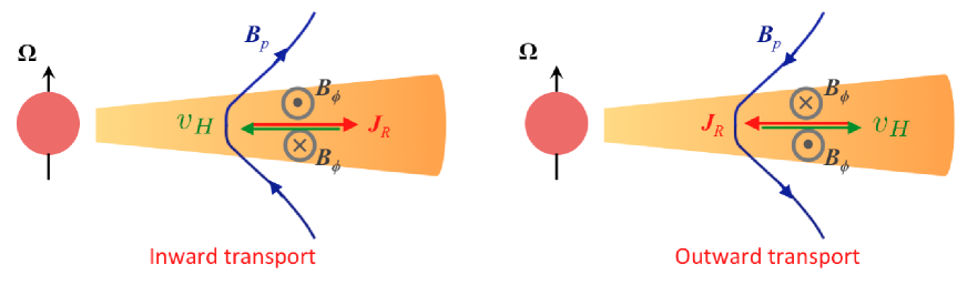
Figure 1.— Illustration of the Hall-effect mediated magnetic flux transport. In the Hall dominated regime, magnetic flux is transported along the direction of the Hall-drift at speed $v_{H}$, which is opposite to the direction radial current $J_{R}$ resulting mainly from the vertical toroidal field gradient. The direction of transport then depends on the polarity of the large-scale poloidal magnetic field relative to the disk rotation axis (marked with $\Omega$). Note that this Cartoon only illustrates magnetic flux transport in the midplane region. The situation elsewhere is different. See text for details.

The electron-ion drift is directly related to current density ${\boldsymbol{J}}=-en_{e}({\boldsymbol{v}}_{e}-{\boldsymbol{v}}_{i})=(c/4\pi)\nabla\times{\boldsymbol{B}}$ . In collisional equilibrium (which is well satisfied in PPDs), the ion-neutral drift velocity is determined by the balance between Lorentz force experienced by the ions and the ion-neutral collisional drag

$$\gamma_{i}\rho\rho_{i}({\boldsymbol{v}}_{i}-{\boldsymbol{v}})=\frac{1}{c}{\boldsymbol{J}}\times{\boldsymbol{B}}\ ,$$ (2)

where $\gamma_{i}$ is the coefficient of momentum transfer between ion-neutral collisions, $\rho$, $\rho_{i}$ are the density of the bulk gas (neutrals) and the ions. In particular, $\gamma_{i}\rho_{i}$ characterizes the frequency for the neutrals to collide with the ions.

More formally, the evolution of magnetic field ${\boldsymbol{B}}$ is described by the induction equation, given by

$$\frac{\partial{\boldsymbol{B}}}{\partial t}=\nabla\times({\boldsymbol{v}}_{e}\times{\boldsymbol{B}})-\frac{4\pi}{c}\nabla\times(\eta_{O}{\boldsymbol{J}})\ ,$$ (3)

where $\eta_{O}$ is Ohmic resistivity. Substituting the electron velocity (1) to the above, one obtains the more familiar expression

$$\frac{\partial{\boldsymbol{B}}}{\partial t}=\nabla\times({\boldsymbol{v}}\times{\boldsymbol{B}})-\frac{4\pi}{c}\nabla\times(\eta_{O}{\boldsymbol{J}}+\eta_{H}{\boldsymbol{J}}\times{\boldsymbol{b}}+\eta_{A}{\boldsymbol{J}}_{\perp})\ ,$$ (4)

where ${\boldsymbol{b}}\equiv{\boldsymbol{B}}/B$ is the unit vector for the magnetic field direction, ${\boldsymbol{J}}_{\perp}=-({\boldsymbol{J}}\times{\boldsymbol{b}})\times{\boldsymbol{b}}$ is the component of ${\boldsymbol{J}}$ that is perpendicular to the magnetic field. The Hall and ambipolar diffusivities (grain-free case) are given by

$$\eta_{H}=\frac{cB}{4\pi en_{e}}\equiv v_{A}l_{H}\ ,\quad\eta_{A}=\frac{B^{2}}{4\pi\gamma_{i}\rho\rho_{i}}\equiv\frac{v_{A}^{2}}{Am\cdot\Omega}\ ,$$ (5)

where we have defined the Hall length $l_{H}$ (Kunz & Lesur, 2013), which is the analog of the ion inertial length in fully ionized plasmas, and the dimensionless AD Elsasser number $Am\equiv v_{A}^{2}/\eta_{A}\Omega$, with $\Omega$ being the disk Keplerian frequency. Both $l_{H}$ and $Am$ have the advantage of being independent of magnetic field strength. The strength of the Hall term is also conveniently measured by the dimensionless Hall Elsasser number defined by $\chi\equiv v_{A}^{2}/\eta_{H}\Omega$, which is field-strength dependent. Note that at fixed ionization fraction $n_{e}/n$, we have $\eta_{O}=$ constant, $\eta_{H}\propto B/\rho$, and $\eta_{A}\propto B^{2}/\rho^{2}$. Therefore, AD becomes progressively more important towards lower density regions.

Using the Hall and AD diffusivities, one can further express the Hall and ambipolar drift velocites as

$${\boldsymbol{v}}_{H}\equiv{\boldsymbol{v}}_{e}-{\boldsymbol{v}}_{i}=-\frac{\eta_{H}}{B}(\frac{4\pi}{c}){\boldsymbol{J}}=-v_{A}\frac{l_{H}\nabla\times{\boldsymbol{B}}}{B}\ ,$$ (6)

$${\boldsymbol{v}}_{AD}\equiv{\boldsymbol{v}}_{i}-{\boldsymbol{v}}=\frac{\eta_{A}}{B}(\frac{4\pi}{c}){\boldsymbol{J}}\times{\boldsymbol{b}}=\frac{(\nabla\times{\boldsymbol{B}})\times{\boldsymbol{B}}}{4\pi\rho\Omega\cdot Am}\ .$$ (7)

From (3), transport of magnetic flux in a laminar flow is given by

$$\begin{split}\frac{d\Phi_{B}(R,z)}{dt}=&-2\pi R{\mathcal{E}}_{\phi}\\ =&-2\pi R\bigg{[}(v_{e,R}B_{z}-v_{e,z}B_{R})+\frac{4\pi}{c}\eta_{O}J_{\phi}\bigg{]}\ .\end{split}$$ (8)

where $\Phi_{B}(R,z)$ is the amount of magnetic flux enclosed within a ring at cylindrical radius $R$ and height $z$, $\mathcal{E}$ is the electric field. In the second equality, the first term corresponds to radial advection of vertical field that directly lead to accumulation or reduction of the enclosed magnetic flux. The second term corresponds to vertical advection of radial field into or out of the ring, which also affects the amount of flux enclosed in the ring. As we will see, both terms contribute to magnetic flux transport.

We focus on the Hall drift in this section. In thin disks, we generally expect the toroidal field to be the dominant field component, and the current density is mainly set by its vertical gradient. Therefore, we expect $J_{R}\gg J_{z}$, and hence the Hall-effect mediated flux transport is dominated by the radial advection term $v_{H,R}B_{z}$. Assuming axisymmetry, we have from (6)

$$v_{H,R}=\frac{\eta_{H}}{B}\frac{\partial B_{\phi}}{\partial z}\ .$$ (9)

We see that the direction of magnetic flux transport is mainly determined by the sign of $\eta_{H}$ (which is positive in general), and the sign of the vertical gradient of the toroidal field.

In disks, the sign of toroidal magnetic field is generally opposite to the sign of radial field because of Keplerian shear. For a large-scale poloidal field that drives an MHD disk wind, the general poloidal field configuration is illustrated in Figure 1. As the poloidal field bends away from the protostar, the system tends to develop oppositely directed toroidal fields above and below the midplane. Therefore, a radial current is generated in the midplane region, and magnetic flux near the midplane is transported to the direction that is opposite to this radial current.

Most interestingly, the direction of flux transport is opposite for poloidal fields with different polarities. Transport is directed inward when poloidal field is aligned with disk rotation, while it is directed outward for the anti-aligned case. We can also estimate the rate of magnetic flux transport. Assuming toroidal field varies on scales of disk scale height $H=c_{s}/\Omega$, where $c_{s}$ is gas sound speed, then we find magnetic flux travels at the radial Hall-drift speed

$$|v_{H,R}|\sim\frac{\eta_{H}}{H}\frac{B_{\phi}}{B}\approx v_{A}\frac{l_{H}}{H}\ ,$$ (10)

where we have taken $B_{\phi}\sim B$. Therefore, if the Hall length $l_{H}$ is comparable to $H$, magnetic flux is transported at about the Alfvén speed near disk midplane. This represents a very significant contribution that was largely overlooked in previous studies.

In comparison, diffusive transport of magnetic flux due to resistivity and AD generally points outward, at the rate of $v_{O,R}\sim\eta_{O}/H$ or $v_{AD,R}\sim\eta_{A}/H$ around the disk midplane (i.e., Lubow et al., 1994, and from Equation (7)). Overall, the three non-ideal MHD effects affect magnetic flux transport in different ways, while the rate of the transport scale with the respective diffusivities in a similar fashion.

While we discussed the physics assuming there were no charged grains, the expressions (6) and (7) are general, with magnetic diffusivities replaced by more complex expressions (Wardle, 2007; Bai, 2011a). Also note that $\eta_{H}$ can change sign for sufficiently strong magnetic field in the presence of charged grains (Xu & Bai, 2016), and in that case, the direction of magnetic flux transport would be reversed.

3. Method

Transport of magnetic flux is intimately connected to the global disk dynamics. We proceed to perform global simulations of PPDs to study magnetic flux transport in a more quantitative and self-consistent manner.

3.1. Simulation Setup

We use Athena++, a newly developed grid-based higher-order Godunov MHD code with constrained transport to conserve the divergence-free condition for magnetic fields (Stone et al., in preparation). It is the successor of the widely used Athena MHD code (Gardiner & Stone, 2005, 2008; Stone et al., 2008), and is highly optimized in several aspects. In particular, it employs flexible grid spacings, allowing simulations to be performed over large dynamical ranges. Geometric source terms in curvilinear coordinate systems (e.g., cylindrical and spherical-polar coordinates) are carefully implemented, which ensures exact angular momentum conservation.

Using Athena++, we solve the standard MHD equations in conservation form

$$\frac{\partial\rho}{\partial t}+\nabla\cdot(\rho{\boldsymbol{v}})=0\ ,$$ (11)

$$\frac{\partial(\rho{\boldsymbol{v}})}{\partial t}+\nabla\cdot\bigg{(}\rho{\boldsymbol{v}}{\boldsymbol{v}}-\frac{{\boldsymbol{B}}{\boldsymbol{B}}}{4\pi}+{\mathsf{P}}^{*}\bigg{)}=-\nabla\Phi\ ,$$ (12)

$$\frac{\partial E}{\partial t}+\nabla\cdot\bigg{[}(E+P^{*}){\boldsymbol{v}}-\frac{{\boldsymbol{B}}({\boldsymbol{B}}\cdot{\boldsymbol{v}})}{4\pi}\bigg{]}=-\Lambda\ ,$$ (13)

where $P$ is gas pressure, $P^{*}=P+B^{2}/8\pi$ is total pressure, $E=P/(\gamma-1)+\rho v^{2}/2+B^{2}/8\pi$ is total energy density, $\gamma$ is the adiabatic index, ${\mathsf{P}}^{*}\equiv P^{*}{\mathsf{I}}$ with ${\mathsf{I}}$ being the identity tensor, $\Phi=-GM/r$ is the gravitational potential of the protostar, and $\Lambda$ is the cooling rate. These equations are coupled with the induction equation (4), which incorporates non-ideal MHD effects, to evolve the magnetic field. Also note that in the code, factors of $4\pi$ are absorbed into the definition of $B$ so that magnetic permeability is $\mu=1$.

With these advantages, we perform 2D global MHD simulations of PPDs in spherical-polar coordinates ($r-\theta$). The radial grid spans from $r=1$ to $100$ in code units with logarithmic grid spacing. The $\theta$ grid extends from the midplane all the way to near the poles (leaving only a $2^{\circ}$ cone at each pole), with non-uniform grid spacing where $\Delta\theta$ increases by a constant factor per grid cell from midplane to pole, with contrasting factor of four between the midplane and the polar region. This allows us to properly resolve the disk, and in the mean time accommodate the MHD disk wind so that the simulation results are not affected by the outer boundary conditions. Note that in spherical-polar grid, $\theta$ increases from $0$ to $\pi$ from the north to the south pole. For notational convenience, we define $\delta\equiv\pi/2-\theta$, namely, the elevation angle about the midplane.

For initial condition, we adopt a self-similar disk density and temperature profiles in the form of $\rho=\rho_{0}(r/R_{0})^{-\alpha}f(\theta)$, $T=P/\rho=T_{0}(r/R_{0})^{-1}g(\theta)$. In code units, we set $\rho_{0}=T_{0}=R_{0}=1$. Further, we take $GM=1$ for the gravity of the central protostar. Once we specify the dimensionless function $g(\theta)$, which corresponds to the square of local disk aspect ratio $(H/r)^{2}$, the density profile can be solved assuming hydrostatic equilibrium. In the $\theta$-direction, it yields

$$\frac{d\ln F}{d\ln\sin\theta}=\frac{GM}{T_{0}R_{0}}\frac{1}{g(\theta)}-(\alpha+1)\ ,$$ (14)

where we have defined $F(\theta)\equiv f(\theta)g(\theta)$. Hydrostatic equilibrium is possible when the right hand side is positive, which limits the maximum value of $g(\theta)$. Force balance in the radial direction determines $v_{\phi}$:

$$v_{\phi}^{2}=\frac{GM-(\alpha+1)T_{0}R_{0}g(\theta)}{r}\ .$$ (15)

Throughout this paper, we choose $\alpha=2$, corresponding to a surface density profile of $\Sigma\propto r^{-1}$.

In this work, we consider modestly thin disks with midplane aspect ratio $H_{\rm mid}/r=0.1$ within $\sim 2H_{\rm mid}$ about the disk midplane. It then increases smoothly towards disk surface and reaches $H/r=0.5$ near the Pole. This allows the gas density to drop much more slowly with $\theta$ and hence alleviates the timestep constraint in the MHD wind zone. Physically, this is motivated by the fact that the wind zone to be strongly heated by external UV and X-rays that becomes significantly hotter than the disk interior (e.g., Glassgold et al., 2004; Walsh et al., 2010). Part of the temperature profile $g(\theta)$ can be found in left panels of Figure 3. We adopt an ideal gas equation of state with adiabatic index $\gamma=5/3$, which appropriate for atomic gas in the wind zone, but the results are insensitive to the choice of $\gamma$. We seek for simple prescriptions of thermodynamics, achieved by a simple cooling prescription (the $\Lambda$ term) that relaxes gas temperature to the initial value at the rate of local Keplerian frequency (based on spherical radius $r$). This prescription also avoids the development of hydrodynamic instabilities (e.g., Nelson et al., 2013).

Poloidal magnetic fields are initialized with vector potential generalized from Zanni et al. (2007)

$$A_{\phi}(r,\theta)=\frac{2B_{z0}R_{0}}{3-\alpha}\bigg{(}\frac{R}{R_{0}}\bigg{)}^{-\frac{\alpha-1}{2}}[1+(m\tan\theta)^{-2}]^{-\frac{5}{8}}\ ,$$ (17)

where $R\equiv r\sin\theta$, and $m$ is a parameter that specifies the degree that poloidal fields bend, with $m\rightarrow\infty$ giving a pure vertical field. Poloidal field is given by ${\boldsymbol{B}}=\nabla\times(A_{\phi}\hat{\phi})$, so that in the midplane, ${\boldsymbol{B}}=B_{z0}\hat{z}(r/R_{0})^{-(\alpha+1)/2}$, maintaining constant ratio of gas to magnetic pressure, defined by plasma $\beta_{0}$. In practice, we choose $m=0.5$, and we have tested that the results are insensitive to the choice of $m$. Fiducially, we choose $\beta_{0}=10^{4}$, appropriate for the outer region of PPDs (Simon et al., 2013a; Bai, 2015), but we also consider stronger and weaker fields in Section 7.

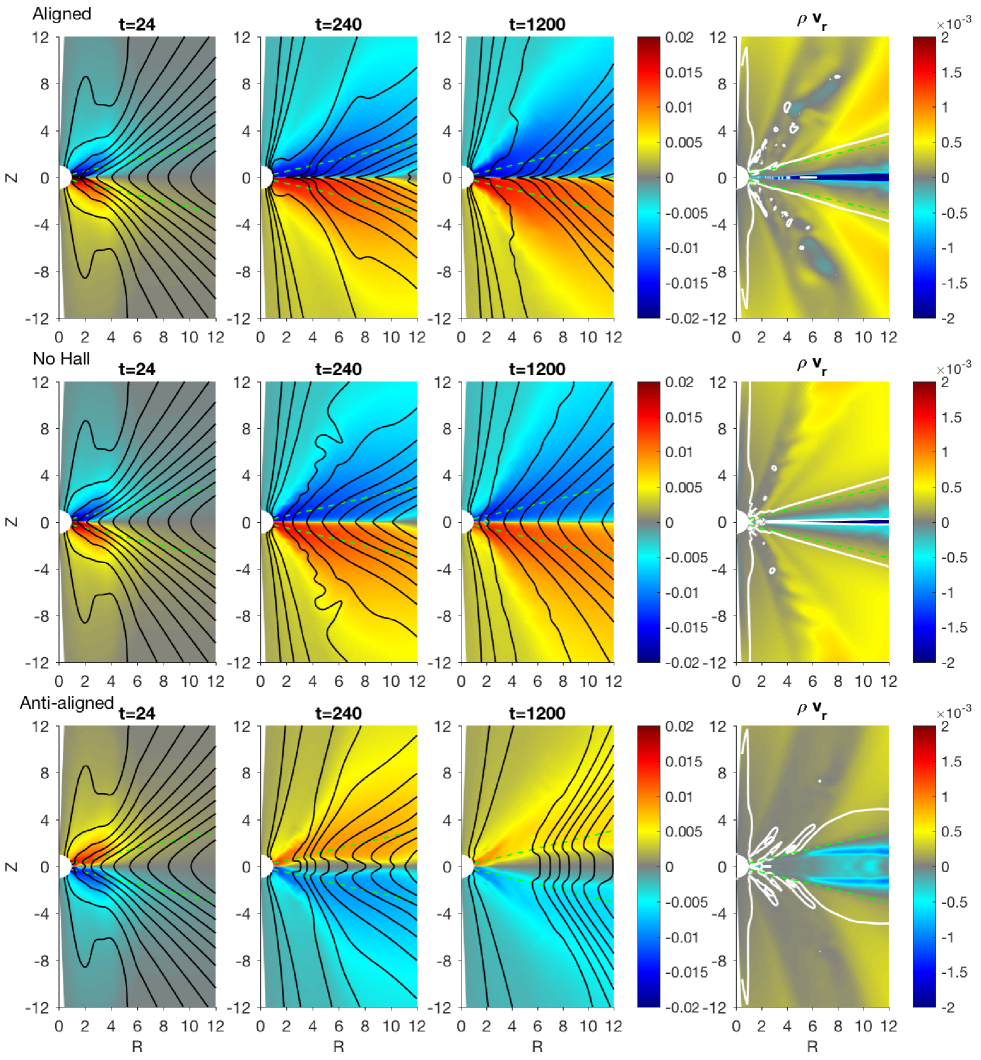
Figure 2.— Left three columns: snapshots of magnetic field configuration represented by equally-spaced contours (of poloidal magnetic flux) and color (toroidal field $RB_{\phi}$) at $t=24$, $240$ and $1200\Omega_{0}^{-1}$. Right column: radial mass flux $\rho v_{r}$ (rescaled by $r^{-\alpha}R^{-1/2}$), overlaid with the Alfvén surface marked by white contours. Top and bottom panels are from simulations with poloidal field aligned and anti-aligned with disk rotation (Fid$\pm$), while the middle panels are from run Fid0 without including the Hall effect. We also include green dashed lines which mark an opening angle of $\delta=0.25$ radian above/below disk midplane, and it roughly corresponds to the transition from the non-ideal MHD dominated disk zone to the disk “corona” where ideal MHD applies.

We have implemented all three non-ideal MHD terms in Athena++. In particular, Ohmic resistivity and ambipolar diffusion are implemented using operator splitting, as in the original Athena code (Bai & Stone, 2011) with super-timestepping (Simon et al., 2013b). We have tested the operator-split implementation of the Hall term following Bai (2014), which was shown to be marginally stable in Cartesian coordinates, and found that it becomes unstable in spherical coordinates. We thus adopt the non-operator-split implementation following Lesur et al. (2014), where the Hall term is incorporated to the Harten-Lax-van Leer (HLL) Riemann solver. While the HLL solver is very diffusive, recent shearing-box simulations using this method (Lesur et al., 2014; Simon et al., 2015) have yielded results consistent with Bai (2014, 2015), who used operator-split and the more accurate HLLD solver (Miyoshi & Kusano, 2005).

In this paper, we focus on regions of PPDs where the Hall effect and ambipolar diffusion are the dominant non-ideal MHD effects, and only include the two terms in our simulations. It typically corresponds to regions of intermediate radii ($r\sim 5-30$ AU) (Wardle, 2007; Bai, 2011a). We set $Am=0.5$ throughout the disk zone (within $\delta\sim\pm 2(H_{\rm mid}/r)$), which is motivated from ionization chemistry calculations (Bai, 2011a, b) where $Am$ is found to be of order unity in the outer disks and becomes smaller towards the inner disk. We take $Am$ to be on the low side which helps suppress the MRI, or at least to significantly reduce its growth rate so that the gas remains largely laminar during the simulations. We further set $l_{H}=2H_{\rm mid}$ in the inner edge of the disk midplane, which is taken from estimates in Bai (2015). The value of $l_{H}$ elsewhere is simply determined from the relation $\eta_{H}/\eta_{A}\propto(B/\rho)^{-1}$, which leads to $l_{H}\propto r^{1/2}\sqrt{\rho}$ for constant $Am$. Beyond $\delta\sim\pm 2(H_{\rm mid}/r)$, we smoothly reduce both Hall and AD diffusivities to zero, mimicking the fact that external far-UV ionization substantially increases the ionization fraction which brings the gas to the ideal MHD regime (Perez-Becker & Chiang, 2011).

Our fiducial simulations are performed with $560\times 216$ grid cells in $r\times\theta$. With non-uniform grid spacing, we achieve a resolution of about $16$ cells per $H_{\rm mid}$ in $\theta$ and $12$ cells per $H_{\rm mid}$ in $r$ around disk midplane. For the fiducial runs, we also conduct simulations using twice the resolution for convergence study. As an initial effort, our simulations are 2D instead of 3D, which on the one hand substantially reduces the computational cost, and moreover, with the MRI largely suppressed/damped due to strong AD (Bai & Stone, 2011), we expect our 2D simulations to capture the essential aspects of disk dynamics.

The outer radial boundary follows from standard outflow boundary prescriptions, where hydrodynamic variables are copied from the last grid zone assuming $\rho\propto r^{-2}$, $v_{\phi}\propto r^{-1/2}$, with $v_{r}$ and $v_{\theta}$ unchanged except that we set $v_{r}=0$ in case of inflow. At the inner radial boundary, hydrodynamic variables are fixed to initial state. We make this choice because the flow near the polar region is presumably originated from the part of the disk that is located within the inner radial boundary, whose dynamics is beyond the reach of the simulation. An outflow-type boundary condition prescription would violate causality, which can become unstable in the presence of magnetic fields and further interfere with the wind flow in the main computational domain. The fixed state boundary condition alleviates the causality issue., and as the gas flow in our simulations is largely laminar, it also guarantees stability. This allows us to pursue our study without being affected from the inner boundary. Magnetic variables in the inner/outer ghost zones are copied from the nearest grid zone assuming $B_{r}\propto r^{-2}$ and $B_{\phi}\propto r^{-1}$, with $B_{\theta}$ unchanged. Moreover, we smoothly reduce the Hall diffusivity to zero within about $H_{\rm mid}$ from the inner radial boundary to avoid dramatic flux transport due to the Hall-drift. Reflection boundary conditions are applied in the $\theta-$boundaries.

Table 1List of Simulation Runs

Run	Polarity	Resolution	$H_{\rm mid}/r$	$\beta_{0}$
Fid+	+	$560\times 216$	0.1	$10^{4}$
Fid0	No Hall	$560\times 216$	0.1	$10^{4}$
Fid$-$	$-$	$560\times 216$	0.1	$10^{4}$
Fid-hires+	+	$1104\times 432$	0.1	$10^{4}$
Fid-hires$-$	$-$	$1104\times 432$	0.1	$10^{4}$
B3+	+	$560\times 216$	0.1	$10^{3}$
B30	No Hall	$560\times 216$	0.1	$10^{3}$
B3$-$	$-$	$560\times 216$	0.1	$10^{3}$
B5+	+	$560\times 216$	0.1	$10^{5}$
B50	No Hall	$560\times 216$	0.1	$10^{5}$
B5$-$	$-$	$560\times 216$	0.1	$10^{5}$

3.2. Simulation Runs

We list all our simulation runs in Table 1. We will focus on our fiducial runs labeled “Fid$\pm$” in the main text, where the $+$/$-$ signs correspond to simulations with poloidal field aligned/anti-aligned with disk rotation. For comparison, we also conduct a run “Fid0”, where we turn off the Hall effect. Results from our high-resolution run are discussed in Appendix A to address numerical convergence. We further discuss the dependence of flux transport rate on the poloidal field strength in Section 7.

We are most interested in the evolution in the inner part of our simulation domain where the Hall effect is dominant at the midplane. The simulations are run for about 400 rotations at the innermost disk radius ($2400\Omega_{0}^{-1}$ where $\Omega_{0}=1$ is the Keplerian frequency at the innermost orbit). This is much longer than the dynamical timescale within $r\lesssim 10-15$ so that the flow structure (e.g., disk winds and accretion flow) is approximately steady. On top of such flow structure, magnetic flux evolves on longer timescales. We call such a situation quasi-steady state, and over the course we can measure magnetic flux evolution. Moreover, with weak magnetization, the rate of angular momentum transport is relatively slow, and within the duration of these simulations, the surface density remains largely unchanged.

4. Overview of Magnetic Flux Evolution

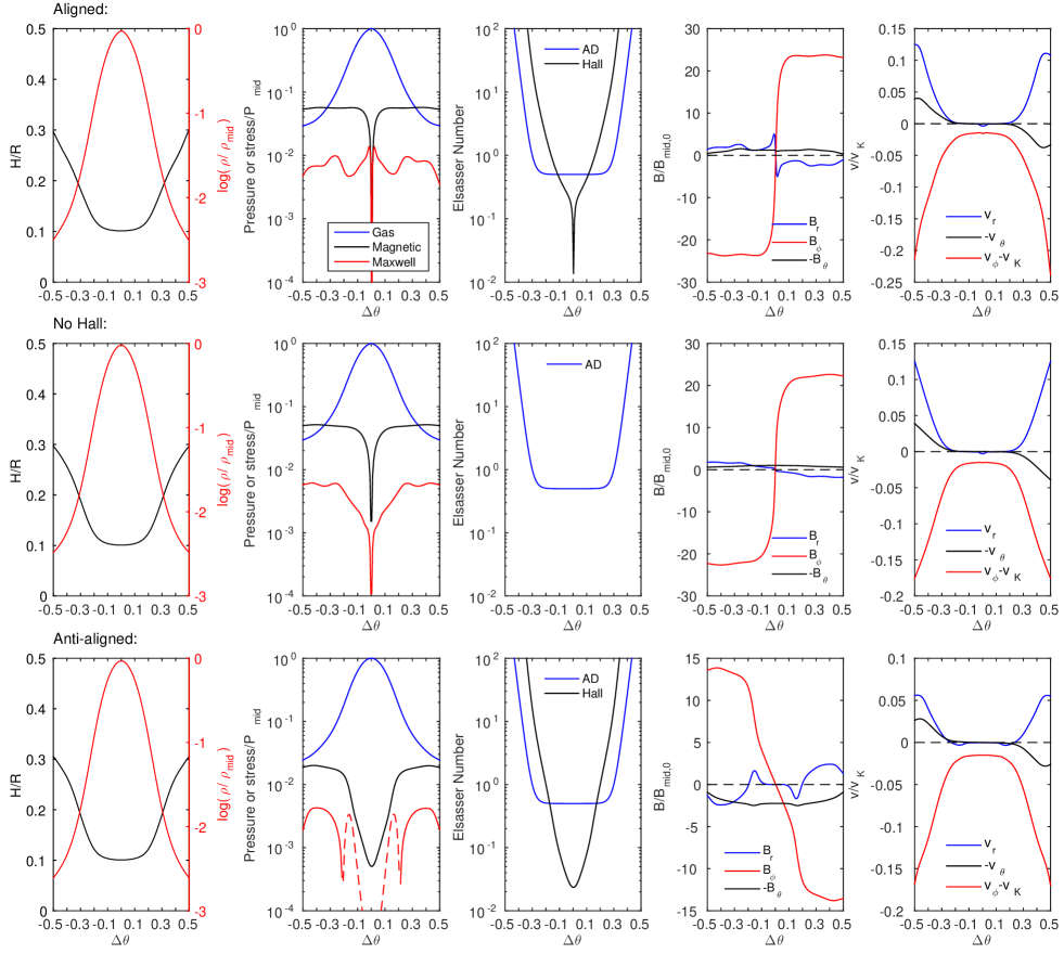
Figure 3.— $\theta$-profiles of various hydrodynamic and magnetic variables (as labeled in the y-axis and legends) at fixed spherical radius $r=8$, measured at time $t=1200\Omega_{0}^{-1}$. Top and bottom panels correspond to results from simulations with aligned and anti-aligned poloidal fields, while the middle panels are from run Fid0 with the Hall term turned off. In these plots, gas density is normalized to midplane gas density, pressure (gas and magnetic) and the Maxwell stress ($-B_{R}B_{\phi}/4\pi$) are normalized to midplane pressure $P_{\rm mid}$, magnetic field strengths are normalized to initial midplane field strength $B_{{\rm mid},0}$, corresponding to plasma $\beta_{0}=10^{4}$, and velocities are normalized to Keplerian velocity $v_{K}$. The insets on the rightmost panels zoom in the accretion velocity $v_{r}$ in the disk zone.

In Figure 2, we show snapshots of magnetic field configurations for all three fiducial runs as the systems evolve. The first snapshot ($t=24\Omega_{0}^{-1}$) is close to the initial state, where initial field configuration is best seen at larger radii. During initial evolution, the outward-bent poloidal field generates oppositely-directed toroidal field above/below midplane due to radial shear, as discussed in Section 2. In the mean time, some of the magnetic flux that penetrates into the inner radial boundary moves into the polar region and becomes more vertical, launching a collimated jet. While the jet is irrelevant to our study (and it is artificial and is not under direct control), it helps stabilize the polar region.

4.1. The Aligned Case

The early evolution follows exactly from the expectations discussed in Section 2. In the aligned case, the Hall effect efficiently transports magnetic flux inward at the midplane, leading to some flux accumulation at the inner radial boundary. Beyond the midplane, however, the toroidal field gradient reverses, and hence magnetic flux is transported outward. The above two processes stretch the poloidal field into a highly radially-elongated configuration, as seen in the second snapshot. As radial field grows, shear produces stronger toroidal field, which in turn leads to faster flux transport, and further growth of the radial field. In fact, the runaway process described here is a global manifestation of the Hall-shear instability (Kunz, 2008), previously discussed in local shearing-box simulations (Lesur et al., 2014; Bai, 2014). Saturation of this instability is owing to additional dissipation, and here AD in our simulations, which we will discuss in more detail in Section 6.2.

Upon saturation, the system achieves a quasi-steady state, with magnetic field bending sharply across the disk midplane. This configuration allows dissipative processes (here AD), which generally tend to straighten field lines, to effectively transport magnetic flux outward in the midplane region. It is the competition between inward transport by the Hall effect and outward transport by AD that determine the overall direction of the transport at the midplane: looking at the third snapshot, the direction of transport is pointing outward.

4.2. The Anti-aligned Case

In the anti-aligned case, the opposite occurs. We see that first, outward transport of magnetic flux takes place at disk midplane as a result of shear-produced toroidal field gradient, as discussed in Section 2. The Hall drift pushes the poloidal field into an unusual configuration which first bends radially inward and then outward. Later on, poloidal field lines around the midplane straighten. This was discussed in Bai (2014), where the situation is exactly the opposite to the aligned case: horizontal components of the field are reduced towards zero instead of undergoing runaway amplification.

Upon achieving a quasi-steady state, poloidal field lines near the midplane region are largely vertical, and the toroidal field gradient across the midplane is greatly reduced but non-zero. With this field configuration, magnetic flux is transported outward almost entirely due to the Hall effect at the midplane, with negligible contribution from AD. Towards disk surface, on the one hand, the Hall effect weakens compared with AD because of the density drop, and on the other hand, the concavely shaped field configuration is more favorable for AD to transport magnetic flux outward. Overall, we find that magnetic flux is systematically transported outward due to the Hall effect at the midplane and AD at the surface.

4.3. The Hall-free Case

Without including the Hall term in run Fid0, we see that besides the production of toroidal field from radial field, there is no significant change of magnetic field configuration from the initial condition. The system reaches a quasi-steady state relatively quickly, with toroidal field generation compensated by ambipolar dissipation in the disk region and outward advection in the disk wind. Despite the significant difference in field configuration, we find that magnetic flux is slowly transported outward at a rate comparable to the Fid$\pm$ runs.

5. Gas Dynamics

In preparation for analyzing the mechanism of magnetic flux transport in more detail, we discuss the gas dynamics in quasi-steady state in this section.

5.1. Quasi-steady State Gas Vertical Profiles

In Figure 3, we show the $\theta$-profiles of various diagnostic quantities of interest measured at spherical radius $r=8$ and time $t=1200\Omega_{0}^{-1}$ (corresponding to the 3rd snapshot in Figure 2). The first (left) column of panels show the density and temperature (expressed in $H/R$) profiles. The latter is well preserved from the initial profile due to our cooling prescription. The density profiles in the bulk disk are largely hydrostatic. Beyond $\delta\sim\pm 3H_{\rm mid}/R$, the density profiles in the aligned and Hall-free cases deviate from the anti-aligned case. This is related to the fact that magnetic pressure exceeds gas pressure beyond about $\delta\sim\pm 3H_{\rm mid}/R$ in the aligned and Hall-free cases, as shown in the second column of panels.

The strength of the Hall and ambipolar diffusion terms are measured by their respective Elsasser numbers, shown in the third panels from left. The AD Elsasser number $Am$ is independent of field strength, and hence the profiles of $Am$ are the same for all cases. As we specified in Section 3, $Am$ is fixed to $0.5$ in the main disk body and it increases towards infinity starting from $2H_{\rm mid}$ above/below midplane. The Hall Elsasser number depends on field strength, and compared with AD, the Hall term is more important in weaker field. Overall, in both aligned and anti-aligned cases, the Hall term dominates within about $1-2H_{\rm mid}$ about midplane.

The forth and fifth panels show the profiles for the three components of magnetic fields and velocities. They are useful for interpreting angular momentum transport in the next subsection. Also note that the azimuthal gas velocity is always sub-Keplerian due to pressure support.

5.2. Transport of Angular Momentum and Mass

In all cases, MHD disk winds are launched. The MHD winds extract disk angular momentum vertically via a wind stress $T_{z\phi}\equiv-B_{z}B_{\phi}/4\pi$ exerted at the disk surface (wind base), leading to an accretion rate $\dot{M}\approx(8\pi R/\Omega)T_{z\phi}$. Approximately, we specify $\delta_{b}=\pm 0.25$ to be the location of the wind base, which roughly corresponds to the location where $Am\sim 1$ and the gas transitions from being dominated by non-ideal MHD to satisfying ideal MHD conditions (which permits efficient wind launching).

We see from Figure 3 that in the aligned case, with $B_{R}$ and $B_{\phi}$ amplified via the Hall shear instability, we measure $T_{z\phi}\approx 8.5\times 10^{-3}P_{\rm mid}$ at $r=8$, where $P_{\rm mid}$ is midplane gas pressure. Without the Hall effect, $B_{\phi}$ is amplified to similar strength but not $B_{R}$, which remains very small. We measure $T_{z\phi}\approx 5.8\times 10^{-3}P_{\rm mid}$, where it is smaller mainly because of smaller $B_{z}$ in this run as a result of magnetic flux evolution. In the anti-aligned case, while horizontal field in the midplane is reduced, $B_{\phi}$ grows steadily towards the surface, and we measure $T_{z\phi}\approx 6.3\times 10^{-3}P_{\rm mid}$ at the wind base, which is only slightly smaller than the aligned case. These results are similar to those discussed in Bai (2014).

The aligned case also produces a relatively strong Maxwell stress $T_{R\phi}=-B_{R}B_{\phi}/4\pi$ around the disk midplane, leading to non-negligible radial transport of angular momentum (magnetic braking). To order of magnitude, the resulting accretion rate is $\dot{M}\sim(2\pi/\Omega)\int_{-\theta_{b}}^{\theta_{b}}T_{R\phi}dz$, which is about a factor $H/R$ less efficient than wind-driven accretion (for similar stress levels). Defining $\alpha=\int_{-\theta_{b}}^{\theta_{b}}T_{R\phi}dz/\int_{-\theta_{b}}^{\theta_{b}}Pdz$, we find $\alpha\approx 0.013$. Comparing $\alpha$ with $T_{z\phi}/P_{\rm mid}$, we see that $\alpha$ is not sufficiently large to offset the $R/H$ factor to dominate angular momentum transport, consistent with local studies (Bai, 2014). In the anti-aligned case, on the other hand, due to the reduction of horizontal field, radial transport is completely negligible.

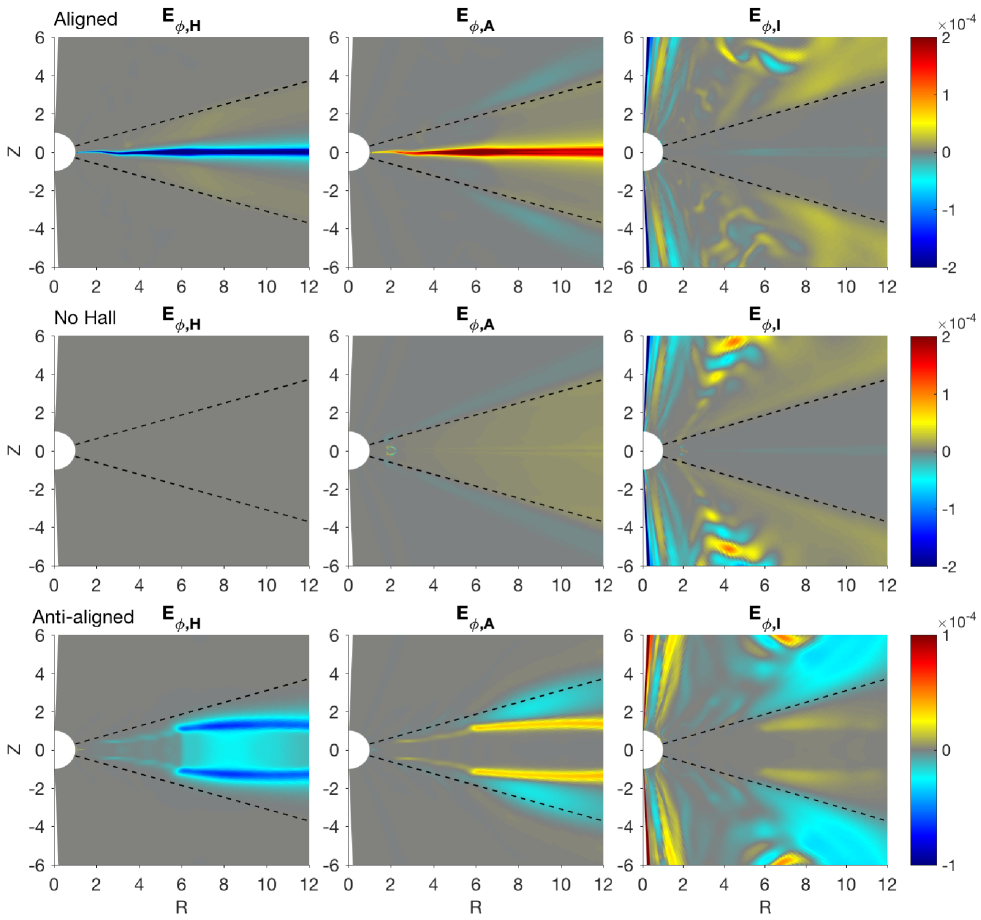
Figure 4.— Spatial distribution of the $\phi$-component of the electric field at time $t=1200\Omega_{0}^{-1}$ in our fiducial simulations, which is directly related to the rate and direction of poloidal magnetic flux transport. It has been rescaled by $R^{-1/2}r^{-(\alpha+1)/2}$. Left, middle and right panels show the contribution from the Hall term, AD, and fluid advection in ideal MHD. Top and bottom panels correspond to aligned and anti-aligned simulations, while the middle panels are from run Fid0 excluding the Hall term. Note that in the aligned case, positive (negative) $E_{\phi}$ means outward (inward) transport, while in the anti-aligned case, the opposite holds.

The accretion flow associated with the wind can be directly seen in the rightmost panels of Figures 2 and 3. Accretion is driven by the torque associated with the vertical gradient of the wind stress, which is the strongest when $B_{\phi}$ varies the fastest. Examining the 4th panels from left in Figure 3, it becomes clear why the mass flux of the accretion flow is mostly concentrated in the midplane in the aligned and Hall-free cases, whereas it is more uniformly distributed with modest concentration around $z=2H_{\rm mid}$ in the anti-aligned case. The total mass accretion rates in all three cases, on the other hand, are comparable because of their similar $T_{z\phi}$ values.

The global distribution of mass flux is best viewed from the rightmost panels of Figure 2. The efficiency of wind-driven accretion is characterized by the ratio of mass loss rate $\dot{M}_{\rm wind}$ to wind-driven accretion rate $\dot{M}_{\rm acc}$. It is closely related to the location of the Alfvén surface, at which poloidal flow velocity is equal to the poloidal Alfvén velocity $v_{Ap}=B_{p}/\sqrt{4\pi\rho}$. For wind launched from radius $R_{0}$, following the field line, one can define the Alfvén radius $R_{A}$ to be the cylindrical radius at the Alfvén surface. Assuming ideal MHD and axisymmetry in steady state, we have (e.g., Spruit, 1996; Bai et al., 2016)

$$\frac{d\dot{M}_{\rm wind}/d\ln R}{\dot{M}_{\rm acc}}=\frac{1}{2}\frac{1}{R_{A}^{2}/R_{0}^{2}-1}\ .$$ (18)

The Alfvén surface obtained in all our simulations is low, indicating large fractional mass loss per unit mass of accretion ($R_{A}/R_{0}\sim 2$). This is related to our adopted low level of magnetization ($\beta_{0}=10^{4}$), and in this case, the winds are largely driven by magnetic pressure gradient (Bai et al., 2016).

We can also see from Figure 2 that in simulations with the Hall effect, the change of magnetic field configuration leads to a segregation of magnetic fluxes in our simulation domain between the inner boundary region and the main disk body. This is largely a numerical artifact because we do not cover disk regions within the inner boundary but still have their magnetic flux contained in the polar region. At $t=1200\Omega_{0}^{-1}$, there is a lack of magnetic flux between $R\sim 1-6$, where both accretion and outflow mass fluxes tend to diminish, and the Alfvén surface is no longer well defined. We will not discuss this region any further. Beyond this region, there are also local concentrations/rarefactions of magnetic flux as a result of intrinsic flux evolution, leading to stronger/weaker local poloidal field (better seen in the anti-aligned case). They make the Alfvén surface move further/retreat, which is consistent with theoretical expectations (Bai et al., 2016).

6. Magnetic Flux Transport: Detailed Analysis

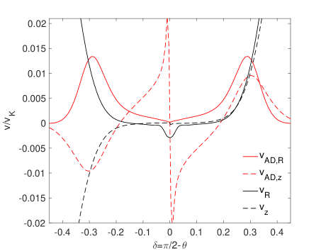
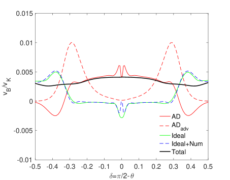
Figure 5.— $\theta$-profiles of various diagnostics that contribute to magnetic flux transport measured at spherical radius $r=8$ at time $t=1200\Omega_{0}^{-1}$ in our Fid0 run (no Hall effect). Left: decomposition of electron velocity into flow velocity $v$ and ambipolar drift velocity $v_{\rm AD}$. Shown are the (cylindrical) radial and vertical components of these velocities, as indicated in the legend. Right: individual terms in ${\mathcal{E}}_{\phi}$ normalized by $v_{K}B_{z}$. The sum of all contributions is shown in the thick black line. The blue dashed line also include contributions from numerical dissipation, and will be discussed in Appendix A. See text in Section 6.1 for details.

With magnetic flux transport obtained self-consistently with the disk gas dynamics, in this section, we analyze in detail the contributions from individual physical effects to the global flux transport. Our starting point is Equation (8). Without explicit resistivity, flux transport is due to the ${\boldsymbol{v}}_{e}\times{\boldsymbol{B}}$ term. We decompose the electron velocity as in (1), and use (6) and (7) to compute the Hall drift and AD drift velocities. The remaining ${\boldsymbol{v}}\times{\boldsymbol{B}}$ term corresponds to fluid advection as in ideal MHD. We pick $t=1200\Omega_{0}^{-1}$ as a fiducial time of evolution, and show the contributions from these three effects individually in Figure 4 for our fiducial runs Fid$\pm$ and Fid0.

6.1. The Hall-free Case

We start from the Hall-free simulation Fid0 as a reference. Together with Figure 4, we further show in Figure 5 with a more detailed analysis at spherical radius $r=8$. On the left panel, we show the $\theta-$profiles of radial and vertical components (in cylindrical coordinates) of ambipolar drift and flow velocities. On the right panel, we show the profile of

$$\frac{v_{B}}{v_{K}}\equiv\frac{{\mathcal{E}}_{\phi}}{v_{K}B_{z}}\ ,$$ (19)

which is dimensionless and can be considered as the effective velocity of flux transport $v_{B}$ normalized by the Keplerian velocity. Overall, upon reaching a quasi-steady state, magnetic flux is transported outward ($v_{B}>0$) at all heights at approximately the same rate. In other words, the system adjusts/relaxes itself (mainly in its magnetic field configuration) in such a way that the rate of transport at all heights converges towards a constant value. We now analyze the contribution from individual physical effects.

6.1.1 Contribution from AD

In the bulk disk, we see from Figure 4 and the right panel of Figure 5 that outward transport is almost completely due to AD. For the contribution from AD, we separate out the term $v_{AD,R}B_{z}$, denoted as $AD_{\rm adv}$, corresponding to the advection of vertical field due to radial component of ambipolar drift. From the left panel of Figure 5, we see that $v_{AD,R}$ is positive, leading to outward flux transport. This transport process is mathematically (though not physically) analogous to outward transport by Ohmic resistivity discussed in the literature, and the resulting ${\mathcal{E}}_{\phi}$ is dominated by $\eta_{A}J_{\phi}(B_{z}^{2}/B^{2})$ (as opposed to $\eta_{O}J_{\phi}$).

However, the rate of transport by this $AD_{\rm adv}$ term is very small near the midplane. Instead, outward flux transport is dominated by the $v_{{\rm AD},z}B_{R}$ term. As we can see from the left panel of Figure 5, AD drift near the midplane is dominated by the vertical component, pointing towards the midplane. This contribution is unique to AD due to its the anisotropic nature. It results from a strong toroidal field gradient, and by order-of-magnitude, it can be a factor $\sim(B_{\phi}/B_{z})^{2}$ stronger than the $AD_{\rm adv}$ term near the midplane.

Physically, this drift motion brings oppositely directed (poloidal and toroidal) magnetic field into the midplane region. While the drift velocity $v_{{\rm AD},z}$ tends to diverge and changes sign at the midplane, this is compensated by the fact that poloidal field lines becomes more vertical (smaller $B_{R}$) near the midplane, and the net rate $v_{{\rm AD},R}B_{z}$ remains finite at the midplane, as can be seen on the right panel of Figure 5. Exactly at the midplane where both poloidal and toroidal fields change sign, the vertical drift velocity vanishes, and outward flux transport there is effectively achieved by reconnection.

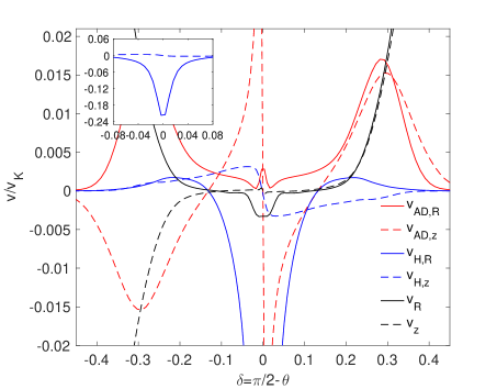
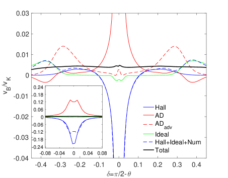
Figure 6.— Same as Figure 5, but for run Fid$+$ that includes the Hall effect with aligned poloidal field geometry. On the left panel, newly added are lines corresponding to radial and vertical Hall-drift velocities $v_{H,R}$ and $v_{H,z}$. On the right panel, newly added are the rate of magnetic flux transport due to the Hall drift. The blue dashed line also include contributions from numerical dissipation, and will be discussed in Appendix A. In both panels, an inset is added zooming in the midplane region.

6.1.2 Contribution from Fluid Advection

Fluid advection is associated with bulk gas motion, and in our case, it consists of the wind-driven accretion flow concentrated at the midplane, and the wind flow itself. The accretion flow drags magnetic flux inward. However, because the midplane is the densest part of the disk, accretion velocity is relatively small. As is shown in the green line on the right panel of Figure 5, its contribution to flux transport is very minor.

In the disk wind zone, we note that in general, fluid advection can accommodate arbitrary rate of flux transport in any direction. If field lines are all anchored at fixed radii (no transport), then wind flows travel along poloidal field lines, together with a series of conservation laws along such field lines (e.g., Spruit, 1996). Non-zero rate of flux transport can be achieved by having the direction of the wind flow deviate from the poloidal field direction. This deviation leads to a direct advection of poloidal flux, corresponding to a non-zero toroidal electric field (Lesur et al., 2013). Therefore, we interpret the outward transport of magnetic flux in the disk wind region mainly as a response to the transport driven in the midplane region, so as to achieve a quasi-steady state field configuration. On the other hand, the self-consistent wind dynamics in our simulation provides the boundary condition for the disk, allowing the field configuration to adjust itself accordingly.

6.1.3 Overall Rate of Flux Transport

In quasi-steady state, the rate of flux transport $v_{B}$ slowly evolves with time, and is weakly dependent on disk radius (see Appendix B). For reference, we quote the value of $v_{B}\approx 4\times 10^{-3}v_{K}$ from our Fid0 run, which corresponds to the rate measured at $r=8$ and $t=1200$ based on Figure 5 averaged within $\delta=\pm 0.3$.

We note that this rate is consistent with a simple order-of-magnitude estimate discussed in Section 2:

$$v_{B}\sim\eta_{A}/H\approx\frac{2}{\rm Am}\frac{1}{\beta}\frac{H_{\rm mid}}{R}v_{K}\ ,$$ (20)

where the plasma $\beta$ is the ratio of gas to total magnetic pressure. We have ${\rm Am}=0.5$, $H_{\rm mid}/R=0.1$ in run Fid0. The plasma $\beta$ depends on field strength. Note that while the initial poloidal field has $\beta_{0}=10^{4}$, in quasi-steady state, toroidal field dominates, and is of the order $\sim 10$ times stronger (see the 4th column of Figure 3) near the midplane. It gives $\beta\sim 10^{2}$, which together yields $v_{B}\sim 4\times 10^{-3}v_{K}$.

6.2. The Aligned Case

We now consider the Hall simulation Fid$+$ with aligned poloidal field, and in Figure 6, we show the contributions to magnetic flux transport from individual terms at $r=8$ and $t=1200$, with the Hall-drift term (6) included. Again, in this quasi-steady state, magnetic flux is transported outward at approximately the same rate at all heights. The role of fluid advection and AD are similar to those discussed in the Hall-free case. Below, we focus on the Hall-effect mediated flux transport.

6.2.1 Hall-effect Mediated Flux Transport

Recall that the Hall effect is most prominent in the midplane (within $\sim\pm 2H_{\rm mid}$), and its relative importance to AD weakens towards disk surface roughly as $\sim 1/\rho$. Therefore, we focus on the bulk disk region.

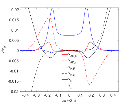
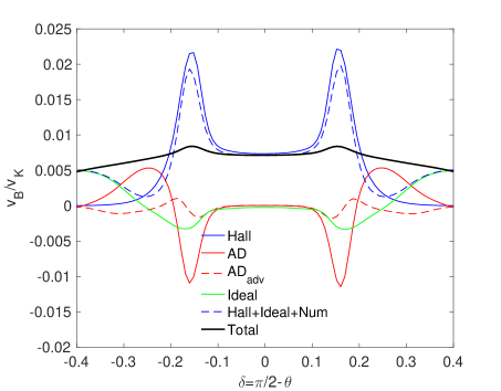
Figure 7.— Same as Figure 6, but for run Fid$-$ that includes the Hall effect with anti-aligned poloidal field geometry.

As discussed in Section 4, the Hall drift drags magnetic flux inward in the midplane while pushes the flux outward above and below. This is confirmed from the top left panel of Figure 4 as well as Figure 6. They further show that inward drag is much faster than outward drift. Inward Hall-drift velocity at the midplane reaches as fast as $\sim 20\%$ of the Keplerian speed! This is largely owing to the strong toroidal field gradient across the midplane as a result of the Hall shear instability. Outward transport above/below the midplane due to the Hall effect is only $\sim 0.1\%v_{K}$, because the (reversed) toroidal field gradient in the upper layer is much smaller, and the Hall diffusivity is also significantly reduced. We have also checked that the Hall-mediated transport is almost entirely due to the $v_{H,R}B_{z}$ term (radial advection of vertical field). This is because the toroidal field gradient across the midplane is the strongest, and hence the radial Hall drift velocity $v_{H,R}$ overwhelms $v_{H,z}$, as seen from the left panel of Figure 6.

The highly stretched field configuration across the midplane allows any dissipative process, in this case AD, to provide outward transport much faster than the Hall-free case. In fact, it is this outward flux transport that eventually terminates the runaway growth of the Hall-shear instability, leading to its saturation. We can see from Figure 6 that outward transport near the midplane is again dominated by the $v_{AD,z}B_{R}$ term. Comparing with the Hall-free case, we see that while $v_{AD,z}$ is only modestly larger, its contribution to ${\mathcal{E}}_{\phi}$ from the $v_{AD,z}B_{R}$ term is much more significant because of the highly radially-stretched field configuration. Its value slightly exceeds the contribution from the Hall term ($v_{H,R}B_{z}$), leading to a net outward transport after significant cancelation. In Appendix A, we further discuss results from our high-resolution run Fid-hires$+$ and show that while numerical dissipation also contributes to the outward flux transport within 2 cells across the midplane, it does not affect the global rate of flux transport.

6.2.2 Overall Direction and Rate of Flux Transport

From Figure 6, we quote the rate of outward flux transport in run Fid$+$ to be $v_{B}\approx 4\times 10^{-3}v_{K}$ measured at $r=8$ and $t=1200$ averaged within $\delta=\pm 0.3$. This is about the same as the Hall-free case, despite the dramatic influence of the Hall effect. We now ask, why is magnetic flux eventually transported outward, and at a rate that is comparable to the Hall-free case?

The direction of flux transport in the midplane region determined by the competition between the Hall-effect-driven inward transport, and outward transport due to AD or other dissipative processes (e.g., resistivity). Based on our earlier discussion, we expect the rate of outward flux transport to increase as the radial field becomes more stretched. In this sense, by adjusting poloidal field configurations, flux transport in both directions with a wide range of rates can be accommodated. Therefore, we expect that the global rate of magnetic flux transport is not determined in the midplane region.

From Figure 6, we see that at vertical hight $\delta\sim 0.1-0.3$ where toroidal field gradient reverses, both the Hall effect and AD lead to outward flux transport yet no other mechanism can provide any significant inward transport. We thus conclude that it is this region that determines the overall rate of flux transport, while other regions (midplane and the wind zone) adjust their field configuration to achieve the same rate of transport in response.

To order-of-magnitude, we may estimate the rate of outward transport owing to the Hall effect using (10), but applied to the intermediate layer between the midplane and the wind zone ($\delta\sim\pm 0.2$ in our case):

$$v_{B}\sim v_{A}\frac{l_{H}}{H}=\sqrt{\frac{2}{\beta}}\frac{l_{H}}{H_{\rm mid}}\frac{H_{\rm mid}}{R}v_{K}\ .$$ (21)

At $r=8$ and $\delta=\pm 0.2$, we can infer from Figure 3 that $\beta\sim 5$, and $l_{H}\sim 0.3H$. We then obtain $v_{B}\sim 2\times 10^{-3}v_{K}$, which reasonably approximates the measured rate of flux transport.

6.3. The Anti-aligned Case

Finally, we discuss the Hall simulation Fid$-$ with anti-aligned poloidal field, and show in Figure 7 the contributions to magnetic flux transport from individual terms at $r=8$ and $t=1200$. With anti-aligned poloidal field, we find that the mechanism of magnetic flux transport, as seen from the decomposition shown in the Figures, is qualitatively different from the Fid0 and Fid$+$ cases.

6.3.1 Contribution from Individual Terms

We start by focusing on the midplane region. As discussed in Section 4, the anti-aligned geometry minimizes the vertical gradients of horizontal magnetic field across the midplane, making poloidal field largely vertical, leaving with only very small toroidal field gradient (Bai, 2014). This field configuration reduces the AD drift and fluid advection velocities to almost zero near the midplane, and they contribute negligibly to magnetic flux transport. The Hall-drift velocity is also substantially reduced compared to the case with aligned poloidal field (by a factor of $\sim 30$), but owing to its direct proportionality to $\partial B_{\phi}/\partial z$, it is the only dominant term present in the midplane. This fact alone dictates that magnetic flux must be transported outward.

Contribution from the Hall term maximizes at around $\delta\sim\pm 0.16$, where the Hall Elsasser number approaches unity. The reason it is located at this height is due to a sudden increase of toroidal field gradient (which can be tracked in Figure 3) and the fact that the Hall term in the region is still strong enough to provide significant Hall drift. This enhanced outward transport is partially canceled by inward transport by AD so that the net rate of transport remains approximately the same as in the midplane. Transport by AD is again dominated by the $v_{AD,z}B_{R}$ term. It transports flux inward in this region because of the unusual poloidal field geometry. While $v_{AD,z}$ still points to the midplane, poloidal fields are bent inward instead of outward, as can be seen in Figure 2.

Toward the disk surface up to $|\delta|\sim 0.25$, the Hall term diminishes and its contribution rapidly falls off. In the mean time, poloidal field configuration returns normal and bends outward, where AD leads to outward transport of magnetic flux as usual. Fluid advection due to wind-driven accretion around $\delta\sim 0.2$ accounts for a higher fraction of the overall rate of transport than the alighed/Hall-free cases, although it still represents a minor contribution. In the wind zone (beyond $\delta=0.3$), fluid advection completely takes over to account for the outward flux transport.

6.3.2 Overall Direction and Rate of Flux Transport

From Figure 7, we quote the rate of outward flux transport in run Fid$+$ to be $v_{B}\approx 7\times 10^{-3}v_{K}$ measured at $r=8$ and $t=1200$ averaged within $\delta=\pm 0.3$. This is about a factor of 2 faster than the Hall-free and aligned cases. To order-of-magnitude, we may estimate the rate of outward transport from (21), but using parameters near the midplane region. We find $l_{H}/H\sim 0.7$, and $\beta\sim 10^{2-3}$, which yields $v_{B}\sim 3-10\times 10^{-3}v_{K}$, consistent with the measured rate of flux transport.

7. Dependence on Poloidal Field Strength

In this Section, we vary the imposed poloidal field strength to $\beta_{0}=10^{3}$ and $10^{5}$ with all other parameters fixed (runs B3x and B5x listed in Table 1 where “x” represents $\pm$ or $0$), and discuss the results jointly with our fiducial runs with $\beta_{0}=10^{4}$.

In Figure 8, we show the measured rate of flux transport $v_{B}$ from these runs. For consistency, for all runs, we measure the rate of flux transport at spherical radius $r=8$ at $t=1200$, averaged in between $\delta=\pm 0.3$. In some of the runs, we find that $v_{B}$ at fixed radius evolves further after $t=1200$, which we will discuss in more detail in Appendix B and argue that the rate measured at relatively early time ($t=1200$) more appropriately reflects the originally imposed disk magnetization.

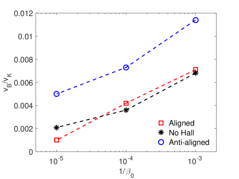
Figure 8.— Rate of outward magnetic flux transport $v_{B}$ as a function of disk magnetization (given by the inverse of midplane plasma $\beta_{0}$). Black asterisks correspond to the Hall-free simulations, and red squares and blue circles correspond to Hall-simulations with aligned and anti-aligned poloidal fields. The rates of transport are measured at $r=8$ and averaged within $\delta=\pm 0.3$.

In all cases, we clearly see that $v_{B}$ increases with stronger magnetization. Moreover, $v_{B}$ in the Hall-free case remains to be very similar to the aligned case, whereas $v_{B}$ in the anti-aligned case is consistently higher by a factor of $\sim 2$.

Qualitatively, the reason behind this trend can be understood from the discussions in Section 2. Given the same magnetic field configuration, we see that the Hall drift speed $v_{B,H}\propto B$, and the AD drift speed $v_{B,AD}\propto B^{2}$ (see also Equations (20), (21)). In Section 6, we have identified that the rate of flux transport is determined by regions at certain heights where the above order-of-magnitude estimates hold, we thus expect that stronger poloidal field leads to faster transport, and vice versa.

We also note that the rate of transport mainly scales with the total field strength $B$ that is dominated by the toroidal component. While total field $B$ increases as net poloidal field strength increases, the relation between the two is highly nonlinear as a result of internal disk dynamics. Usually, total $B$ increases more slowly than net poloidal field. This explains that in Figure 8, $v_{B}$ increases more slowly than the net field strength.

In the conventional theory of magnetic flux transport where flux transport is attributed to a balance between viscously driven accretion and outward diffusion by resistivity (Lubow et al., 1994), the rate of transport does not explicitly depend on disk magnetization. In particular, for outward transport by Ohmic resistivity, the rate of transport is independent of field strength for a given field configuration. Within the conventional framework, field strength does indirectly affect the rate of transport by its feedback on disk dynamics, especially when poloidal field is strong (e.g., Guilet & Ogilvie, 2012, 2013). Note that the level of magnetization in all our simulations are relatively weak (since $\beta_{0}\geq 10^{3}$), yet the dominant role played by the Hall effect and AD already leads to clearly identifiable dependence of flux transport rate on disk magnetization.

8. Discussion

This work represents the first effort to study magnetic flux transport in PPDs that incorporates more complex and realistic physics. Our simulations have adopted idealized prescriptions in disk structure (constant $H/R$), non-ideal MHD diffusivities (constant $Am$), together with a smooth transition at disk surface. The purpose is to make the problem reasonably well defined so as to identify important pieces of physics.

8.1. Relation to the Conventional Theory

The conventional advection-diffusion framework has been developed further over the past decade, aiming to address the issue of rapid loss of magnetic flux in thin accretion disks expected from Lubow et al. (1994). Majority of the works have been constructed under the assumption that the accretion disk is turbulent as a result of the MRI, with the effect of the MRI turbulence represented by an effective viscosity and resistivity. Their ratio, called the magnetic Prandtl number, has been measured to be of order unity in full MRI turbulence (Guan & Gammie, 2009; Lesur & Longaretti, 2009; Fromang & Stone, 2009), and it leads to the conventional wisdom that magnetic flux is transported outward for thin accretion disks. More recently, disk vertical structure and boundary conditions have been realized to play an important role in the flux transport process. Bisnovatyi-Kogan & Lovelace (2007), Rothstein & Lovelace (2008) and Bisnovatyi-Kogan & Lovelace (2012) postulate that the surface of the accretion disks can be largely laminar because it is magnetically dominated (e.g., Miller & Stone, 2000) and the MRI is suppressed. They suggest that inward advection of magnetic flux can be easily achieved in the non-turbulent, conducting surface layer. Guilet & Ogilvie (2012, 2013) presented a family of asymptotic solutions in the thin disk limit assuming that disk magnetic field is largely vertical. They find that magnetic flux can be advected inward much faster than the mass flux due to the large radial velocities at the low-density disk surface, and this effect can substantially alleviate the issue of magnetic flux loss by outward diffusion. With prescriptions of disk resistivity/viscosity, the theories have also been applied to PPDs (Okuzumi et al., 2014; Takeuchi & Okuzumi, 2014; Guilet & Ogilvie, 2014), and reasonable steady-state distributions of magnetic flux have been obtained.

These updated theories may be better applicable to fully MRI turbulent disks (e.g., black hole accretion disks), although they remain to be tested against simulations. However, when applied to PPDs, these theories suffer from several major issues. First, PPDs are largely laminar with the MRI suppressed or significantly damped (Bai & Stone, 2013b; Bai, 2013; Simon et al., 2013a; Gressel et al., 2015). Second, while physical resistivity is present in PPDs, as considered in Guilet & Ogilvie (2013) and Okuzumi et al. (2014), it dominates only in very limited regions in PPDs. The Hall effect and AD, which govern almost the entire range of radii in PPDs, are missing. Third, in the presence of poloidal field threading the disk, MHD disk wind launching appears inevitable (Suzuki & Inutsuka, 2009; Suzuki et al., 2010; Fromang et al., 2013; Bai & Stone, 2013a, b; Lesur et al., 2013), which has been ignored in most of the conventional studies (with the exception of Guilet & Ogilvie series, who partially incorporated its effect). Besides the wind-driven accretion process, the wind provides necessary surface boundary conditions that are not easily incorporated into the existing framework.

Our work advances our understanding of magnetic flux transport in PPDs over several major aspects. First, we have shown that the Hall effect and AD play distinct roles in magnetic flux transport that are dramatically different from resistivity. Because of the anisotropic nature of the Hall effect and AD, magnetic flux transport depends on the gradient of magnetic fields in all directions, with the most sensitive being the vertical gradient of the toroidal field. It implies that the process of magnetic flux transport is strongly coupled with the gas dynamics of the disk itself, leading to substantial complications. Second, our simulations have self-consistently incorporated the launching and propagation of MHD disk winds. On the one hand, it provides realistic “boundary conditions” at disk surfaces, and on the other hand, it allows the wind dynamics to adjust itself to match the rate of flux transport demanded from the disk.

Our results are also in line with some of the updated conventional theories in that flux transport is mediated by different mechanisms at different heights in the disk. Therefore, a complete theory of magnetic flux transport in PPDs must properly take into account the disk vertical structure, and use realistic vertical profiles of magnetic diffusivities.

8.2. Implications on Disk Formation

Magnetic flux is not only the controlling factor for PPD evolution, it also plays a fundamental role controlling the process of star and disk formation. Molecular clouds are known to be relatively strongly magnetized (Crutcher, 2012), and the star and disk formation processes naturally inherit some magnetic flux from the parent cloud. The role of AD has been discussed extensively in the literature in the context of “magnetic flux problem” of star formation during core collapse (see McKee & Ostriker, 2007 for a thorough review and references therein), where substantial magnetic flux must be lost. The Hall effect has generally been considered not to be important during core collapse, as long as there is no significant rotation to develop strong toroidal magnetic field (e.g., Kunz & Mouschovias, 2010).

Formation of rotationally supported PPDs, on the other hand, unavoidably involve winding-up of poloidal fields into toroidal fields, leading to significant magnetic braking. Further loss of magnetic flux is necessary to enable disk formation (Mellon & Li, 2008, and see Li et al., 2014 for a review and references therein). In this context, all non-ideal MHD effects prove to be important (Li et al., 2011; Krasnopolsky et al., 2011; Tomida et al., 2013). In particular, it has recently been found that AD enables significant magnetic flux loss (Tomida et al., 2015), and further inclusion of the Hall effect leads to a bimordality on the initial disk size depending on the polarity of the background magnetic field with respect to initial angular momentum vector (Tsukamoto et al., 2015; Wurster et al., 2016).

While we have focused on magnetic flux transport in PPDs, the same physics is applicable in the disk formation process. Tsukamoto et al. (2015) and Wurster et al. (2016) have found that a larger disk is formed when field polarity is anti-aligned, whereas aligned field polarity leads to smaller initial disk size, although the underlying physical reasons were not addressed. The fact that both polarities lead to disk formation agrees with our conclusion that magnetic flux is systematically transported outward. Our finding that the anti-aligned case loses flux faster than the aligned case implies that less magnetic flux would be preserved in the former case, and hence weaker magnetic braking. Therefore, we expect larger/smaller disk to be formed in the anti-aligned/aligned cases, offering an explanation for the findings of Tsukamoto et al. (2015) and Wurster et al. (2016).

8.3. Global Evolution of Protoplanetary Disks

Our results serve as a first step towards a better understanding of magnetic flux transport in PPDs, which largely controls global disk evolution. We discuss below how our results should be interpreted for this purpose, as well as cautions that must be exercised.

We first note that the rate of transport obtained in this work is rather high. For $v_{B}/v_{K}=5\times 10^{-3}$, magnetic flux depletion timescale would be on the order of only $\sim 30$ local orbits, which amounts to only $\sim 10^{3}$ years at the distance of 10 AU! However, owing to various caveats to be summarized in the next subsection, especially the artificial prescriptions of non-ideal MHD diffusivities, the rate of flux transport measured in this work is unlikely to be realistic, and readers should not take the values too seriously. As already emphasized, we aim to clarify the physics before incorporating more realistic prescriptions, which are left for future works.

The trend that the rate of outward flux transport increases with increasing net field strength suggests that the strongly magnetized phase of PPDs, if present, is short lived because of relatively rapid loss of magnetic flux. The bulk of the disk lifetime is likely associated with relatively weak disk magnetization. Because stronger magnetic flux leads to higher accretion rate, our results further imply that the rapid phase of disk evolution with high accretion rate is brief, and accretion rate decreases with time. As the loss of magnetic flux slows down over time, we expect the deceleration of accretion rate to slow down as well. Although still premature to be incorporated to global disk evolution models, our results also suggest that the assumption that magnetic flux is conserved in recent global disk evolution models is unlikely to be valid, while models with decreasing magnetic flux is more appropriate (see e.g., Armitage et al., 2013; Bai, 2016).

At this point, the speculations above are qualitative. With the current tools available, it has become feasible to conduct realistic simulations of PPDs that incorporate more realistic prescriptions, and we expect the physics learned from this work to be greatly beneficial for future explorations. While we have ignored Ohmic resistivity in this study, making it more applicable to the outer regions of PPDs ($\gtrsim 10$ AU), it is the inner disk ($\lesssim 15$ AU) that is expected to be almost fully laminar (Bai, 2013, 2014). A further complication in the inner disk is that the vertical structure can become asymmetric (e.g, Bai & Stone, 2013b; Gressel et al., 2015). With Ohmic resistivity dominating the midplane region and suppressing current, the strong current layer typically lies at a few $\sim H_{\rm mid}$ offset from the midplane. It may be present in only one side of the midplane, leading to an asymmetric current distribution. When the Hall effect is turned on, it was found in local shearing-box simulations that maintaining a physical wind geometry with poloidal field lines bending away from the star can hardly be achieved (Bai, 2014). Based on what we have found, such asymmetric current distribution would lead to asymmetric magnetic flux transport due to the Hall drift. It is unclear whether a quasi-steady state is possible in such an asymmetric configuration, which is an intriguing question for future investigations.

8.4. Caveats and Limitations

As a first study, our simulations are subject to several caveats and limitations, some of which are already mentioned earlier in the text and Appendix A. We briefly summarize them below.

A major limitation of the present work is the assumption of axisymmetry. While it is likely a valid approximation in the inner disk ($r\lesssim 10-15$ AU, Bai, 2013, 2014), extending it to the outer disk can be problematic because the MRI can develop in both midplane (weak) and surface (strong), as has been previously studied in local shearing-box simulations (Perez-Becker & Chiang, 2011; Simon et al., 2013b, a; Bai, 2015). Additional contribution from turbulence introduces further complications and uncertainties that need to be addressed using full 3D simulations.

Another limitation arises from the use of the HLL solver. We have shown in Appendix A that the rate of flux transport converges with resolution, implying that the system is able to self-adjust to compensate for the excess numerical dissipation from the HLL solver. However, it also implies that in reality, the strong current layer would be much thinner, which raises concerns on its stability. Corrugation of the strong current layer has already been observed in some of our simulations, which may eventually destroy the strong current layer. Similar phenomenon has also been observed in 3D shearing-box simulations of Bai (2015), where the midplane strong current layer corrugates but without destroying itself. In general, properly capturing this dynamical behavior would require full 3D simulations, as well as using less diffusive solvers (at limited resolution). Therefore, further improvements on the Hall MHD algorithm would be highly desirable.

For clarity, we have chosen simplified disk models (including thermodynamics) and prescribed the non-ideal MHD diffusion coefficients. The prescriptions are motivated from yet do not necessarily reflect realistic disk conditions. In particular, the non-ideal MHD diffusivities are mainly determined by the disk ionization level, and the vertical extent where they dominate largely depends on the penetration depth of external far-UV radiation. None of these processes are included. For instance, around $5$ AU, the disk would be thinner with $H_{\rm mid}/r\sim 0.05$ instead of $0.1$, and non-ideal MHD dominates up to $\sim 4H_{\rm mid}$ for typical FUV penetration depth, instead of $\sim 2.5H_{\rm mid}$. Therefore, we caution on the interpretation of the measured rates of flux transport. Investigations are underway to use more realistic prescriptions that incorporate ionization chemistry, far-UV irradiation, flared disk geometry, etc. (see also initial results from Béthune et al., 2016).

9. Summary

In this work, we have studied the transport of poloidal magnetic flux in PPDs, which has recently been realized to play a crucial role in long-term disk evolution, and hence many aspects of planet formation. We focus on the regime where the Hall effect and AD are the dominant non-ideal MHD effects, which is applicable to a wide range of radii in PPDs. We first demonstrate that the Hall effect in PPDs can lead to rapid transport of magnetic flux as a result of the Hall-drift, which derives from a radial current produced from the vertical gradient of toroidal magnetic field. For typical MHD wind field geometry with toroidal field generated from Keplerian shear, we expect that in the midplane region, magnetic flux should be transported inward (outward) for poloidal field aligned (anti-aligned) with respect to the disk rotation axis. The rate of transport is proportional to the Hall diffusivity and the vertical gradient of the toroidal field, and can be on the order of the Alfvén velocity for typical disk conditions.

We then proceed to perform 2D MHD simulations in spherical polar coordinates in the $r-\theta$ plane using the state-of-the-art Athena++ MHD code. Our simulations properly resolve the thin disk and in the mean time have the $\theta-$domain extend to near the polar region to accommodate the launching and propagation of MHD disk winds. We have implemented and incorporated the Hall effect and AD in the simulations, with a simple prescription of diffusivities that is roughly applicable to $\sim 5-30$ AU. Our simulation results are valid as long as the disk is largely laminar, which is likely the case in a wide range of radii for typical PPDs.

Overall, we find that upon reaching quasi-steady states, magnetic flux is systematically transported outward at approximately the same rate at all heights above/below the midplane at a given disk radius. The detailed mechanism and the rate of transport, however, are different for different poloidal field polarities. The direction and rate of magnetic flux transport is mainly determined by the physics in the bulk disk, where the transport is mediated by the Hall effect and AD by means of the Hall drift and ambipolar drift. Wind-driven accretion plays only a minor role in this process. In the wind zone, flux transport is simply mediated by fluid advection as a response to the flux transport in the bulk disk, which is achieved by having the wind velocity vectors deviate from magnetic field lines.

For poloidal field aligned with disk rotation, we find

• The Hall drift transports magnetic flux inward very rapidly at the midplane, and outward relatively slowly in the disk upper layer. These processes stretch the poloidal field into a radially elongated configuration as a global manifestation of the Hall shear instability.

• At the midplane, inward transport due to the Hall drift is compensated by outward transport by AD (dominated by vertical ambipolar drift). Towards disk upper layer, both the Hall effect and AD contribute to outward transport, which mainly determines the direction and rate of flux transport.

For poloidal field anti-aligned with disk rotation, we find

• In the midplane region, horizontal field components are suppressed, and magnetic flux transport is governed by the Hall drift, which points outward.

• Towards disk upper layer, poloidal field lines bend first radially inward due to outward flux transport at the midplane, and then outward to launch the disk wind. The Hall effect (outward), AD, and wind-driven accretion (inward) all contribute to flux transport.

In both cases, and within the parameters explored in this work, we find that outward transport is inevitable because there are always regions where only outward transport is possible. These include the disk upper layer in the aligned case, and the midplane region in the anti-aligned case. Overall, we find that the anti-aligned case leads to faster outward transport than the aligned case and the Hall-free case by a factor of $\sim 2$. More strongly magnetized disk leads to faster outward transport.

With our fiducial simulation parameters, we find the net rate of outward transport is uncomfortably large. We emphasize that the main purpose of this work is to demonstrate basic physics, and caution on directly applying the measured rate of flux transport to PPDs. The resolution to this issue likely lies in the caveats discussed in Section 8.4, namely, the need for realistic disk model with self-consistent ionization-recombination chemistry, and role of the MRI turbulence which may operate at the surface layer of the outer disk. Our preliminary studies have found that when realistic diffusivity profile is applied for the inner disk, the rate of flux transport is significantly slower. In addition, we have also found that in fully MRI turbulent thin disks, transport of magnetic flux is dominated by the turbulent disk surface via the “coronal mechanism”, which points radially inward (Beckwith et al., 2009).

Through this work, we point out and clarify the important roles played by the Hall effect and AD on the transport of magnetic flux in PPDs that have been missing in conventional theories of magnetic flux transport in accretion disks. The anisotropic nature of these non-ideal MHD effects makes the flux transport process coupled with essentially all components of magnetic field gradients (particularly the vertical gradient of toroidal field), and hence the entire disk gas dynamics. The problem is intrinsically global and multi-dimensional, requiring MHD disk winds to be well accommodated, and disk vertical structure to be appropriately resolved. Future explorations should focus on simulations with more realistic prescriptions of magnetic diffusivities and disk thermodynamics. We expect the physics learned from this work to provide key insight as more complexity is built up towards more realistic studies of PPD.

Appendix A A: Strong Current Layer at the Midplane and Resolution Study

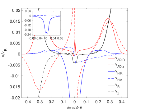
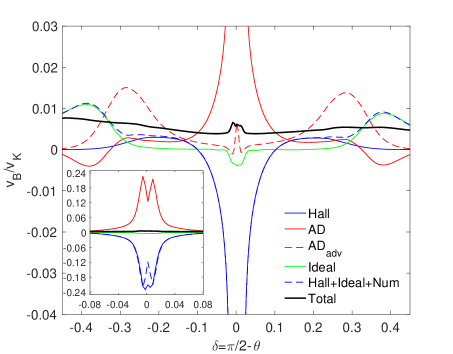
Figure 9.— Same as Figure 6, but for run Fid-hires$+$ where the resolution is doubled.

In both Fid0 and Fid$+$ runs, the systems are characterized by a thin, strong current layer across the midplane. This thin current layer dissipates shear-generated toroidal magnetic field via reconnection, and leads to outward transport of poloidal magnetic flux. In our simulations, some of the reconnection and outward transport are due to numerical dissipation. In this Appendix, we discuss the physics of the strong current layer, and show that the presence of numerical dissipation does not affect the global rate of magnetic flux transport.

Due to the use of the very diffusive HLL solver, numerical dissipation can become significant in the strong current layer. In our simulations, we also extract the electric field ${\mathcal{E}}_{\phi}$ that is actually used to update the magnetic field via constrained transport. Their $\theta-$profiles are shown as blue dashed lines on the right panels of Figures 5 and 6 for run Fid0 and Fid$+$, respectively. They contain contributions from the combination of the ideal MHD and Hall (in run Fid$+$) terms, as well as numerical diffusion. We further zoom in the profiles near the midplane shown in the insets. By comparing the sum of blue and green lines with the blue dashed line, we confirm that numerical dissipation is negligible except in the vicinity of the midplane, which we will focus on below.

Significant numerical dissipation is localized within $\pm 2$ cells above/below the midplane. In run Fid$+$, inward drag due to the Hall term (blue) is nearly twice stronger than intrinsic outward transport due to AD, with the rest of the outward transport owing to numerical dissipation. This dissipation can be effectively considered as a resistivity. It produces additional ${\mathcal{E}}_{\phi}$ from a toroidal current $J_{\phi}$, which mainly results from the vertical gradient of $B_{R}$, as poloidal field lines bend. Accordingly, the more radially stretched field configuration in run Fid$+$ leads to much faster numerical transport of magnetic flux compared with the Fid0 run.

To assess whether numerical dissipation affects the global rate of magnetic flux transport, we further show in Figure 9 the analysis of the high-resolution run Fid-hires$+$ where grid resolution is doubled. We see that contributions from individual terms to magnetic flux transport are almost identical between runs Fid$+$ and Fid-hires$+$. In particular, the global rates of transport from the two runs are almost the same (run Fid-hires$+$ yields a value that is $\sim 10\%$ larger at the particular snapshot). This result suggests that the system is able to adjust its local magnetic field configuration to adapt to different levels of numerical dissipation at the midplane without affecting the global rate of flux transport, which gives us confidence in our simulation results.

In reality, in the absence of numerical dissipation, the outward transport at the midplane must be mediated by physical dissipation. Such physical dissipation can be Ohmic resistivity, which is progressively more important towards the in the inner region of PPDs, and would act in a way analogous to numerical dissipation. In our case, dissipation is provided by AD. Note that the $v_{AD,z}B_{R}$ term discussed in Section 6.1.1 vanishes at the midplane, and hence outward transport at the midplane must be due to the radial advection term $v_{AD,R}B_{z}$. Although this term appears to be negligible in run Fid0 (see Figure 5), its becomes more noticeable in run Fid$+$ where the radial field becomes more stretched (see Figure 6). With higher resolution, the significance of this term grows further as the current sheet becomes sharper, as seen from Figure 9. In the limit of no numerical dissipation, we thus expect this radial AD-drift to be able to account for the entire outward transport at the midplane region. In the mean time, we caution that the development of much sharper current sheet poses concerns on its stability, which is an important caveat yet is beyond the scope of the current investigation.

Finally, we briefly comment that in the anti-alignd case, because the magnetic field profile is much smoother, we find that the electric field returned from the HLL solver matches very well with the total electric field evaluated separately from fluid advection and the Hall term, as can be seen from Figure 7. We have also conducted a higher-resolution run Fid-hires$-$ and confirm that the results agree very well with the fiducial run Fid$-$.

Appendix B B: Global Magnetic Flux Evolution

In most parts of this paper, we conduct analysis at snapshots where magnetic flux evolution is in quasi-steady state. In this Appendix, we discuss the time evolution of magnetic flux during such “quasi-steady” state.

In Figure 10, we show the time evolution of $v_{B}$ defined in (19), measured at different disk locations including both the disk midplane and upper layer ($\delta=\pm 0.2$ from midplane, averaged), for our runs Fid$\pm$ and Fid0. We see that initially, magnetic flux evolves at different rates between the midplane and the surface. Later on, after about $\sim 4$ local orbital time at each radius, transport rates at the midplane and upper layer converge and a quasi-steady state is achieved. Note that the measured rates at midplane and upper layers do not necessarily match exactly because they are connected to different field lines.

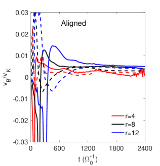
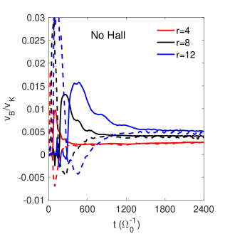
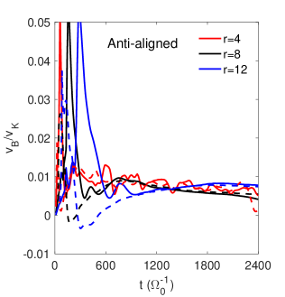
Figure 10.— Time evolution of the rate of magnetic flux transport $v_{B}\equiv{\mathcal{E}}_{\phi}/B_{z}$ in our fiducial run Fid$+$ (left), Fid0 (middle) and Fid$-$ (right) at different disk locations as a function of time. Solid lines correspond to the midplane regions, and dashed lines correspond to the location $\delta=0.2$ above/below the midplane (averaged). Line colors represent different disk radii, as indicated in the legend.

In both the Hall-free case and the aligned case at $r=8$, we see that the rate of flux transport $v_{B}$ remains approximately constant over longer-term evolution. This fact justifies our approach of measuring $v_{B}$ only at fixed snapshots. In the anti-aligned case, however, $v_{B}$ shows some further time evolution. At our fiducial radius $r=8$, $v_{B}$ slowly decreases with time, and is reduced by $\sim 40\%$ from time $t=1200$ to the end of simulation at $t=2400$. The main reason for this reduction is that outward flux transport is the fastest for run Fid$-$, and towards later time, there is a deficit of flux at small radii. For instance, we see in Figure 2 for run Fid$-$ at $t=1200$, magnetic flux is already substantially depleted in the region around $r=4-6$, and shortly afterwards, the $r\sim 8$ region is also affected. Because of this, the inner disk becomes less strongly magnetized towards later time, leading to slower flux transport according to Section 7. Similarly, the measured $v_{B}$ at $r=4$ in the aligned and anti-aligned cases shows more variability towards later time. This is again due to flux depletion/segregation at that radius, as can be seen in Figure 2. Therefore, we expect that $v_{B}$ measured at earlier times more reliably reflects the true rate of transport at the imposed level of magnetization.

The normalized rate of transport $v_{B}/v_{K}$ also shows some radial dependence. In the Hall-free case, our simulation setup guarantees that the physics is independent of disk radius, and hence one might expect $v_{B}/v_{K}$ should be independent of $r$. In practice, we see that $v_{B}/v_{K}$ is modestly different at different radii, and is slower at smaller radius. Without this normalization, on the other hand, we find $v_{B}$ itself is approximately the same across the range of radii between $r=4-12$. In the aligned and anti-aligned case where the Hall effect is included, the measured $v_{B}$ at $r=8$ and $r=12$ also show some difference along their evolutionary paths. Theoretically, magnetic flux transport is intrinsically a global phenomenon, where the dynamics at different radii can affect each other. Moreover, with magnetic flux constantly evolving, flux distribution across the disk also varies with time, and there is no guarantee that the rate of transport has to be constant in time and radius. As an initial study of magnetic flux transport, we do not intend to evolve the system for much longer, nor to address the evolutionary effects in further detail. We simply note here that the rate of flux transport we have measured should only be considered as a reference, and can be subject to uncertainties associated with global conditions.

References

- Armitage et al. (2013) Armitage, P. J., Simon, J. B., & Martin, R. G. 2013, ApJ, 778, L14
- Bai (2011a) Bai, X.-N. 2011a, ApJ, 739, 50
- Bai (2011b) —. 2011b, ApJ, 739, 51
- Bai (2013) —. 2013, ApJ, 772, 96
- Bai (2014) —. 2014, ApJ, 791, 137
- Bai (2015) —. 2015, ApJ, 798, 84
- Bai (2016) —. 2016, ApJ, 821, 80
- Bai & Stone (2011) Bai, X.-N. & Stone, J. M. 2011, ApJ, 736, 144
- Bai & Stone (2013a) —. 2013a, ApJ, 767, 30
- Bai & Stone (2013b) —. 2013b, ApJ, 769, 76
- Bai et al. (2016) Bai, X.-N., Ye, J., Goodman, J., & Yuan, F. 2016, ApJ, 818
- Balbus & Hawley (1991) Balbus, S. A. & Hawley, J. F. 1991, ApJ, 376, 214
- Beckwith et al. (2009) Beckwith, K., Hawley, J. F., & Krolik, J. H. 2009, ApJ, 707, 428
- Béthune et al. (2016) Béthune, W., Lesur, G., & Ferreira, J. 2016, arXiv:1612.00883
- Bisnovatyi-Kogan & Lovelace (2007) Bisnovatyi-Kogan, G. S. & Lovelace, R. V. E. 2007, ApJ, 667, L167
- Bisnovatyi-Kogan & Lovelace (2012) —. 2012, ApJ, 750, 109
- Crutcher (2012) Crutcher, R. M. 2012, ARA&A, 50, 29
- Fromang et al. (2013) Fromang, S., Latter, H., Lesur, G., & Ogilvie, G. I. 2013, A&A, 552, A71
- Fromang & Stone (2009) Fromang, S. & Stone, J. M. 2009, A&A, 507, 19
- Gardiner & Stone (2005) Gardiner, T. A. & Stone, J. M. 2005, Journal of Computational Physics, 205, 509
- Gardiner & Stone (2008) —. 2008, Journal of Computational Physics, 227, 4123
- Glassgold et al. (2004) Glassgold, A. E., Najita, J., & Igea, J. 2004, ApJ, 615, 972
- Gressel et al. (2015) Gressel, O., Turner, N. J., Nelson, R. P., & McNally, C. P. 2015, ApJ, 801, 84
- Guan & Gammie (2009) Guan, X. & Gammie, C. F. 2009, ApJ, 697, 1901
- Guilet & Ogilvie (2012) Guilet, J. & Ogilvie, G. I. 2012, MNRAS, 424, 2097
- Guilet & Ogilvie (2013) —. 2013, MNRAS, 430, 822
- Guilet & Ogilvie (2014) —. 2014, MNRAS, 441, 852
- Königl et al. (2010) Königl, A., Salmeron, R., & Wardle, M. 2010, MNRAS, 401, 479
- Krasnopolsky et al. (2011) Krasnopolsky, R., Li, Z.-Y., & Shang, H. 2011, ApJ, 733, 54
- Kunz (2008) Kunz, M. W. 2008, MNRAS, 385, 1494
- Kunz & Lesur (2013) Kunz, M. W. & Lesur, G. 2013, MNRAS, 434, 2295
- Kunz & Mouschovias (2010) Kunz, M. W. & Mouschovias, T. C. 2010, MNRAS, 408, 322
- Lesur et al. (2013) Lesur, G., Ferreira, J., & Ogilvie, G. I. 2013, A&A, 550, A61
- Lesur et al. (2014) Lesur, G., Kunz, M. W., & Fromang, S. 2014, A&A, 566, A56
- Lesur & Longaretti (2009) Lesur, G. & Longaretti, P.-Y. 2009, A&A, 504, 309
- Li et al. (2014) Li, Z.-Y., Banerjee, R., Pudritz, R. E., Jørgensen, J. K., Shang, H., Krasnopolsky, R., & Maury, A. 2014, Protostars and Planets VI, 173
- Li et al. (2011) Li, Z.-Y., Krasnopolsky, R., & Shang, H. 2011, ApJ, 738, 180
- Lubow et al. (1994) Lubow, S. H., Papaloizou, J. C. B., & Pringle, J. E. 1994, MNRAS, 267, 235
- McKee & Ostriker (2007) McKee, C. F. & Ostriker, E. C. 2007, ARA&A, 45, 565
- Mellon & Li (2008) Mellon, R. R. & Li, Z.-Y. 2008, ApJ, 681, 1356
- Miller & Stone (2000) Miller, K. A. & Stone, J. M. 2000, ApJ, 534, 398
- Miyoshi & Kusano (2005) Miyoshi, T. & Kusano, K. 2005, Journal of Computational Physics, 208, 315
- Nelson et al. (2013) Nelson, R. P., Gressel, O., & Umurhan, O. M. 2013, MNRAS, 435, 2610
- Okuzumi et al. (2014) Okuzumi, S., Takeuchi, T., & Muto, T. 2014, ApJ, 785, 127
- Perez-Becker & Chiang (2011) Perez-Becker, D. & Chiang, E. 2011, ApJ, 735, 8
- Rothstein & Lovelace (2008) Rothstein, D. M. & Lovelace, R. V. E. 2008, ApJ, 677, 1221
- Salmeron et al. (2011) Salmeron, R., Königl, A., & Wardle, M. 2011, MNRAS, 412, 1162
- Sano & Stone (2002a) Sano, T. & Stone, J. M. 2002a, ApJ, 570, 314
- Sano & Stone (2002b) —. 2002b, ApJ, 577, 534
- Simon et al. (2013a) Simon, J. B., Bai, X.-N., Armitage, P. J., Stone, J. M., & Beckwith, K. 2013a, ApJ, 775, 73
- Simon et al. (2013b) Simon, J. B., Bai, X.-N., Stone, J. M., Armitage, P. J., & Beckwith, K. 2013b, ApJ, 764, 66
- Simon et al. (2015) Simon, J. B., Lesur, G., Kunz, M. W., & Armitage, P. J. 2015, MNRAS, 454, 1117
- Spruit (1996) Spruit, H. C. 1996, in NATO ASIC Proc. 477: Evolutionary Processes in Binary Stars, ed. R. A. M. J. Wijers, M. B. Davies, & C. A. Tout, 249–286
- Stone et al. (2008) Stone, J. M., Gardiner, T. A., Teuben, P., Hawley, J. F., & Simon, J. B. 2008, ApJS, 178, 137
- Suzuki & Inutsuka (2009) Suzuki, T. K. & Inutsuka, S.-i. 2009, ApJ, 691, L49
- Suzuki et al. (2010) Suzuki, T. K., Muto, T., & Inutsuka, S.-i. 2010, ApJ, 718, 1289
- Takeuchi & Okuzumi (2014) Takeuchi, T. & Okuzumi, S. 2014, ApJ, 797, 132
- Tomida et al. (2015) Tomida, K., Okuzumi, S., & Machida, M. N. 2015, ApJ, 801, 117
- Tomida et al. (2013) Tomida, K., Tomisaka, K., Matsumoto, T., Hori, Y., Okuzumi, S., Machida, M. N., & Saigo, K. 2013, ApJ, 763, 6
- Tsukamoto et al. (2015) Tsukamoto, Y., Iwasaki, K., Okuzumi, S., Machida, M. N., & Inutsuka, S. 2015, ApJ, 810, L26
- Walsh et al. (2010) Walsh, C., Millar, T. J., & Nomura, H. 2010, ApJ, 722, 1607
- Wardle (1999) Wardle, M. 1999, MNRAS, 307, 849
- Wardle (2007) —. 2007, Ap&SS, 311, 35
- Wardle & Koenigl (1993) Wardle, M. & Koenigl, A. 1993, ApJ, 410, 218
- Wardle & Salmeron (2012) Wardle, M. & Salmeron, R. 2012, MNRAS, 422, 2737
- Wurster et al. (2016) Wurster, J., Price, D. J., & Bate, M. R. 2016, MNRAS, 457, 1037
- Xu & Bai (2016) Xu, R. & Bai, X.-N. 2016, ApJ, 819, 68
- Zanni et al. (2007) Zanni, C., Ferrari, A., Rosner, R., Bodo, G., & Massaglia, S. 2007, A&A, 469, 811