IRAS 18153$-$1651: an H ii  region with a possible wind bubble blown by a young main-sequence B star

Abstract

We report the results of spectroscopic observations and numerical modelling of the H ii  region IRAS 18153$-$1651. Our study was motivated by the discovery of an optical arc and two main-sequence stars of spectral type B1 and B3 near the centre of IRAS 18153$-$1651. We interpret the arc as the edge of the wind bubble (blown by the B1 star), whose brightness is enhanced by the interaction with a photoevaporation flow from a nearby molecular cloud. This interpretation implies that we deal with a unique case of a young massive star (the most massive member of a recently formed low-mass star cluster) caught just tens of thousands of years after its stellar wind has begun to blow a bubble into the surrounding dense medium. Our two-dimensional, radiation-hydrodynamics simulations of the wind bubble and the H ii  region around the B1 star provide a reasonable match to observations, both in terms of morphology and absolute brightness of the optical and mid-infrared emission, and verify the young age of IRAS 18153$-$1651. Taken together our results strongly suggest that we have revealed the first example of a wind bubble blown by a main-sequence B star.

1 Introduction

Hot massive stars are sources of fast line-driven winds (Snow & Morton 1976; Puls, Vink & Najarro 2008), whose interaction with the circum- and interstellar medium results in the origin of bubbles and shells of various shapes and scales (Johnson & Hogg 1965; Lozinskaya & Lomovskij 1982; Chu, Treffers & Kwitter, 1983; Dopita et al. 1994). Since most (if not all) massive stars form in a clustered way (Lada & Lada 2003; Gvaramadze et al. 2012), the wind bubbles produced by individual members of star clusters are unobservable because they merge into a single much more extended structure – a superbubble (McCray & Kafatos 1987). Numerous examples of such superbubbles (with diameters ranging from several tens of pc to kpc scales) were revealed in H$\alpha$ photographic surveys of the Magellanic Clouds and other nearby galaxies (e.g. Davies, Elliott & Meaburn 1976; Meaburn 1980; Courtes et al. 1987; Hunter 1994).

To produce a well-shaped circular bubble or shell a massive star should be isolated from the destructive influence of winds from other massive stars (cf. Nazé et al. 2001). To achieve this, it should leave the parent cluster either because of a few-body dynamical encounter with other massive stars (e.g. Poveda, Ruiz & Allen 1967; Oh & Kroupa 2016) or binary supernova explosion (e.g. Blaauw 1961; Eldridge, Langer & Tout 2011), or it should be the only massive star in the parent cluster. In the first case, the wind bubble around the star running away from its birth place rapidly becomes elongated (Weaver et al. 1977) and transforms into a bow shock (van Buren & McCray 1988) if the star is moving supersonically with respect to the local interstellar medium (ISM). Stellar motion alone is hence the main reason that closed structures around hydrogen-burning massive field stars are not observed. The only known possible exception is the Bubble Nebula (e.g. Christopoulou et al. 1995; Moore et al. 2002), which is produced by the runaway O6.5(n)fp (Sota et al. 2011) star BD+60 2522, whose luminosity class, however, is unknown because of the peculiar shape of the He ii $\lambda$4686 line. The origin of this nebula might be attributed to a situation in which a bow-shock-producing star encounters a density enhancement (cloudlet) on its way, resulting in a temporal formation of a closed bubble with the star located near its leading edge.

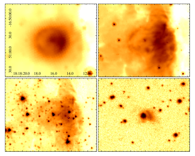
Figure 1: From left to right, and from top to bottom: Spitzer MIPS $24\,\mu$m and IRAC 8 and 3.6 $\mu$m, and SHS H$\alpha$+[N ii] images of IRAS 18153$-$1651 and its central stars (the scale and orientation of the images are the same). The coordinates are in units of RA (J2000) and Dec. (J2000) on the horizontal and vertical scales, respectively. At a distance of 2 kpc, 1 arcmin corresponds to $\approx$0.57 pc.

In the second case, the wind-blowing star is the only massive star (a B star of mass of $8-10\,\rm\,M_{\odot}$) in a star cluster of mass of about $100\,\rm\,M_{\odot}$ (e.g. Kroupa et al. 2013). Such stars with their weak winds produce momentum-driven bubbles (Steigman, Strittmatter & Williams 1975) in the dense material of the parental molecular cloud, which could be detected under favourable conditions, e.g. if the cluster was formed near the surface of the cloud. In this paper, we report the discovery of an optical arc within the circular mid-infrared shell (known as IRAS 18153$-$1651) and argue that it represents the edge of a young ($\sim 10^{4}$ yr) wind bubble produced by a main-sequence B star residing in a low-mass star cluster. In Section 2, we present the images of the arc, IRAS 18153$-$1651 and two stars associated with them, as well as review the existing data on these objects. In Section 3, we describe our optical spectroscopic observations of the arc and the two stars. In Section 4, we classify the stars and model their spectra. In Section 5, we derive some parameters of the arc and propose a scenario for the origin of the arc and the shell around it. In Section 6, we present and discuss results of numerical modelling, which we carried out to support the scenario. We summarize and conclude in Section 7.

2 IRAS 18153$-$1651 and its central stars

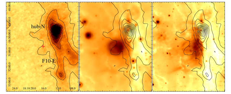
Figure 2: Left: ATLASGAL 870 $\mu$m image of the region around IRAS 18153$-$1651, showing filamentary structures and a density enhancement (hub–N) at $\approx$1.5 arcmin to the north-west from the position of stars 1 and 2 (indicated by a red cross). Middle and right: Spitzer MIPS $24\,\mu$m and IRAC 8 $\mu$m images of the same region with the 870 $\mu$m image overlayed in black contours. The coordinates are in units of RA (J2000) and Dec. (J2000) on the horizontal and vertical scales, respectively. At a distance of 2 kpc, 1 arcmin corresponds to $\approx$0.57 pc. See text for details.

The nebula, which is the subject of this paper, was serendipitously discovered in the archival data of the Spitzer Space Telescope during our search for bow shocks generated by OB stars running away from the young massive star clusters NGC 6611 and NGC 6618 embedded in the giant H ii  regions M16 and M17, respectively (for motivation and some results of this search, see Gvaramadze & Bomans 2008; cf. Gvaramadze et al. 2014a). The Spitzer data we used were obtained with the Multiband Imaging Photometer for Spitzer (MIPS; Rieke et al. 2004) within the framework of the 24 and 70 Micron Survey of the Inner Galactic Disk with MIPS (Carey et al. 2009) and with the Spitzer Infrared Array Camera (IRAC; Fazio et al. 2004) within the Galactic Legacy Infrared Mid-Plane Survey Extraordinaire (Benjamin et al. 2003).

In the MIPS 24 $\mu$m image the nebula appears as a limb-brightened, almost circular shell of radius $\approx$27 arcsec, with the western edge brighter than the other parts of the shell (see Fig. 1, upper left panel). This image also shows the presence of a point-like source, which is somewhat offset from the geometric centre of the shell in the north-west direction. In the SIMBAD data base the nebula is named IRAS 18153$-$1651, and we will use this name hereafter. At the distance of IRAS 18153$-$1651 of 2 kpc (see below), 1 arcsec corresponds to $\approx$0.01 pc, so that the linear radius of the shell is $\approx$0.26 pc.

IRAS 18153$-$1651 and the point source within it are also visible in all (3.6, 4.5, 5.8 and $8.0\,\mu$m) IRAC images (Fig. 1). In these images, the nebula lacks the circular shape and has a more complicated appearance. At 8 $\mu$m one still can see a more or less circular shell, whose west side overlaps with a bar-like structure stretched in the north-south direction. At shorter wavelengths, both the shell and the “bar" become more diffuse. This morphology and the brightness asymmetry of the shell at 24 $\mu$m indicate that the nebula is interacting with a dense medium in the west. This inference is supported by the data of the APEX Telescope Large Area Survey of the Galaxy (ATLASGAL; Schuller et al. 2009). Fig. 2 presents the ATLASGAL 870 $\mu$m image of the region centred on IRAS 18153$-$1651 (left-hand panel) and the Spitzer 24 and 8 $\mu$m images of the same region (middle and right-hand panels, respectively) with the 870 $\mu$m image overlayed in black contours. In the ATLASGAL image one can see two filaments of cold dense gas intersecting each other in a nodal point (dubbed “hub–N" in Busquet et al. 2013; see below for more detail), while comparison of this image with the two other ones shows that IRAS 18153$-$1651 is apparently interacting with the hub–N and one of the filaments (see also below).

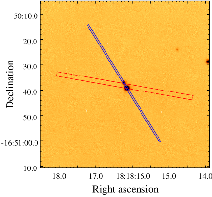
Figure 3: GMOS $g\prime$-band acquisition image of the central stars of IRAS 18153$-$1651, separated from each other by $\approx$2.3 arcsec or $\approx$0.02 pc in projection. The brightest of the stars is star 1. The relative positions of the GMOS and TWIN slits are shown by a solid (blue) and a dashed (red) rectangle, respectively. The widths of the rectangles of 0.75 and 2.1 arcsec correspond to the widths of the slits.

The point source in IRAS 18153$-$1651 can also be seen in all ($J,H,K_{\rm s}$) Two-Micron All Sky Survey (2MASS) images (Skrutskie et al., 2006) as well as in the images provided by the Digitized Sky Survey II (DSS-II) (McLean et al. 2000). The IRAC images clearly show that this source is composed of two nearby stars (see also Fig. 3). The coordinates of these stars, as given in the GLIMPSE Source Catalog (I + II + 3D) (Spitzer Science Center 2009), are: RA(J2000)=$18^{\rm h}18^{\rm m}16\aas@@fstack{s}21$, Dec.(J2000)=$-16\degr 50\arcmin 38\aas@@fstack{\prime\prime}8$ (hereafter star 1) and RA(J2000)=$18^{\rm h}18^{\rm m}16\aas@@fstack{s}28$, Dec.(J2000)=$-16\degr 50\arcmin 36\aas@@fstack{\prime\prime}7$ (hereafter star 2). This catalogue also provides the IRAC band magnitudes for stars 1 and 2 separately. The two stars are also resolved by the the UKIDSS Galactic Plane Survey (Lucas et al. 2008), which gives for them $H$- and $K$-band magnitudes. The total $B$- and $V$-band magnitudes of the two stars are, respectively, 15.84$\pm$0.05 and 14.14$\pm$0.05 (Henden et al. 2016). The details of the stars are summarized in Table 1, to which we also added their spectral types, effective temperatures and surface gravities, based on our spectroscopic observations and spectral analysis (presented in Sections 3 and 4, respectively).

Table 1: Details of two stars in the centre of IRAS 18153$-$1651. The spectral types, SpT, effective temperatures, $T_{\rm eff}$ and surface gravities, $\log g$, are based on our spectroscopic observations and spectral analysis. The coordinates and IRAC photometry are from the GLIMPSE Source Catalog (I + II + 3D) (Spitzer Science Center 2009). The $H$ and $K$ photometry is from Lucas et al. (2008).

	star 1	star 2
SpT	B1 V	B3 V
$\alpha$ (J2000)	$18^{\rm h}18^{\rm m}16\aas@@fstack{s}21$	$18^{\rm h}18^{\rm m}16\aas@@fstack{s}28$
$\delta$ (J2000)	$-16\degr 50\arcmin 38\aas@@fstack{\prime\prime}8$	$-16\degr 50\arcmin 36\aas@@fstack{\prime\prime}7$
$H$ (mag)	10.28$\pm$0.02	11.16$\pm$0.02
$K$ (mag)	9.39$\pm$0.02	10.89$\pm$0.02
$[3.6]$ (mag)	9.00$\pm$0.14	—
$[4.5]$ (mag)	8.98$\pm$0.15	—
$[5.8]$ (mag)	8.83$\pm$0.08	10.14$\pm$0.21
$T_{\rm eff}$ (kK)	22$\pm$2	20$\pm$2
$\log g$	4.2$\pm$0.2	4.4$\pm$0.2

The DSS-II images of IRAS 18153$-$1651 show diffuse emission to the west of stars 1 and 2, extending to the edge of the 24 $\mu$m shell. This emission is also clearly seen in the H$\alpha$+[N ii] image (see Fig. 1) obtained in the framework of the SuperCOSMOS H-alpha Survey (SHS; Parker et al. 2005), which also reveals a clear arcuate structure located at about 12 arcsec (or 0.11 pc in projection) from the stars (note that these stars are not in the geometric centre of the arc; see Section 6.2 for discussion of this issue). The orientation of the arc suggests that it could be shaped by the winds of the central stars and that is what has motivated us to carry out the research presented in this paper.

A literature search showed that the region containing IRAS 18153$-$1651 has been studied quite extensively during the last years (Busquet et a. 2013, 2016; Povich et al. 2016; Santos et al. 2016). These studies, however, only briefly touch IRAS 18153$-$1651 and are mostly devoted to environments of this object. Below we review some relevant information about IRAS 18153$-$1651.

IRAS 18153$-$1651 is a part of the infrared dark cloud G14.225-0.506 (identified with Spitzer by Peretto & Fuller 2009), which, in turn, is a central region of the south-west extension of the massive star-forming region M17 (M17 SWex; Povich & Whitney 2010). Using Spitzer and 2MASS data, Povich & Whitney (2010) concluded that M17 SWex is a precursor to an OB association and that this cloud as a whole will produce $>200$ B stars and perhaps not (m)any O stars. Chandra observations of G14.225-0.506 confirmed that M17 SWex currently hosts no O-type stars (Povich et al. 2016). Observational evidence suggests that M17 SWex is located in the Carina-Sagittarius arm at a distance of 2 kpc (Povich et al. 2016). In what follows, we adopt this distance for IRAS 18153$-$1651 as well.

Radio observations of the dense NH₃ gas in G14.225-0.506 by Busquet et al. (2013) showed that this cloud consists of a net of eight molecular filaments, some of which intersect with each other in two regions of enhanced density (named hub–N and hub–S). IRAS 18153$-$1651 is located at about 1.5 arcmin south-east from one of these two nodal points (hub–N) and is bounded from the west side by a filament (named F10–E) stretching for $\approx$2.5 arcmin from the hub–N to the south (see fig. 2 in Busquet et al. 2013 and Fig. 2). Busquet et al. (2013) attributed the origin of the filaments to the gravitational instability of a thin layer threaded by a magnetic field. Polarimetric observations of background stars at optical and near-infrared wavelengths showed that the magnetic field lines in G14.225-0.506 are perpendicular to most of the filaments and to the (elongated) cloud as a whole (Santos et al. 2016), which further supports the possibility that the regular magnetic field plays an important role in the formation of parallel filaments observed in M17 SWex and other star-forming regions. Interestingly, Santos et al. (2016) found that the magnetic field lines are not perpendicular to the filament F10–E and hub–N (which is also elongated in the north-south direction) and suggested that this discrepant behaviour might be caused by expansion of the H ii  region IRAS 18153$-$1651. Additional evidence suggesting the interaction between IRAS 18153$-$1651 and the filament F10–E and hub–N was presented in Busquet et al. (2013, 2016).

The detection of numerous young stellar objects (Povich & Whitney 2010) and H₂O masers (Jaffe, Güsten & Downes 1981; Wang et al. 2006) in M17 SWex (including G14.225-0.506) points to ongoing star formation in this region, while the presence of several bright IR sources, of which IRAS 18153$-$1651 (with its bolometric luminosity of $\sim 10^{4}\,\rm\,L_{\odot}$ and number of Lyman continuum photons per second of $<1.5\times 10^{46}$; Jaffe, Stier & Fazio 1982) is one of the brightest, implies that a number of massive stars have already formed there. Chandra X-ray Observatory imaging study of M17 SWex revealed that IRAS 18153$-$1651 contains one of the two richest concentrations of X-ray sources detected in this star-forming region (Povich et al. 2016). Povich et al. (2016) suggested that IRAS 18153$-$1651 might represent a site for massive cluster formation, and noted that the infrared and radio continuum luminosities of this H ii  region indicate that it is powered by a B1-1.5 V star. Similarly, Busquet et al. (2016) mentioned unpublished VLA 6cm observations of IRAS 18153$-$1651, which reveal “a cometary H ii  region ionized by a B1 star with the head of the cometary arch pointing toward hub–N". Our spectroscopic observations of stars 1 and 2 confirm that IRAS 18153$-$1651 is powered by a B1 V star (see the next section) and suggest that this H ii  region indeed contains a recently formed star cluster (see Section 5).

3 Spectroscopic observations

To classify the central stars of IRAS 18153$-$1651 and clarify the nature of the optical arc, we obtained long-slit spectra with the Gemini Multi-Object Spectrograph South (GMOS-S) and the Cassegrain Twin Spectrograph (TWIN) of the 3.5-m telescope in the Observatory of Calar Alto (Spain).

3.1 Gemini-South

To obtain spectra of stars 1 and 2, we used the Poor Weather time at Gemini-South under the programme ID GS-2011B-Q-92. GMOS-S provided coverage from 3800 to 6750 Å  with a resolving power of $\approx$3000. The spectra were collected on 2012 May 7 under good seeing conditions ($\approx$0.6 arcsec), but some thick clouds (extinction around 1 mag). The slit of width of 0.75 arcsec was aligned along stars 1 and 2, i.e. with a position angle (PA) of PA=$31\aas@@fstack{\circ}5$, measured from north to east. The desired signal-to-noise ratio of $\sim$150 was achieved with a total exposure time of 9$\times$150 s. The bias subtraction, flat-fielding, wavelength calibration and sky subtraction were executed with the GMOS package in the Gemini library of the iraf software. In order to fill the gaps in GMOS-S s CCD, the observation was divided into three series of exposures obtained with a different central wavelength, i.e. with a 5 Å  shift between each exposure. The extracted spectra were obtained by averaging the individual exposures, using a sigma clipping algorithm to eliminate the effects of cosmic rays. The average wavelength resolution is $\approx$0.46 Å  pixel^-1 (full width at half-maximum (FWHM) $\approx$4.09 Å), and the accuracy of the wavelength calibration estimated by measuring the wavelength of 10 lamp emission lines is 0.061 Å. A spectrum of the white dwarf H600 was used for flux calibration and for removing the instrument response. Unfortunately, due to the weather conditions, any absolute measurement of the flux is not possible.

3.2 Calar Alto

An additional spectrum of IRAS 18153$-$1651 was obtained with TWIN on 2012 July 12 under the programme ID H12-3.5-013. Three exposures of 600 s were taken. The set-up used for TWIN consisted of the gratings T08 in the first order for the blue arm (spectral range 3500–5600 Å) and T04 in the first order for the red arm (spectral range 5300–7600 Å) which provide a reciprocal dispersion of 72 Å ${\rm mm}^{-1}$ for both arms. The resulting FWHM spectral resolution measured on strong lines of the night sky and reference spectra was 3.1–3.7 Å. The Calar Alto observation was mostly intended to get a spectrum of the optical arc. Correspondingly, the slit of $240\times 2.1$ arcsec² was oriented at PA=80$\degr$ to cross the brightest part of the arc. The seeing was variable, ranging from $\simeq$1.5 to 2.0 arcsec. Spectra of He–Ar comparison arcs were obtained to calibrate the wavelength scale and the spectrophotometric standard star BD+$33\degr$ 2642 (Oke 1990) was observed at the beginning of the night for flux calibration.

The primary data reduction was done using iraf: the data for each CCD detector were trimmed, bias subtracted and flat corrected. The subsequent long-slit data reduction was carried out in the way described in Kniazev et al. (2008). The blue and red parts of the spectra were reduced independently for all three exposures, then aligned along the rows using the IRAF apall task, and finally summed up.

4 Stars 1 and 2: spectral classification and modelling

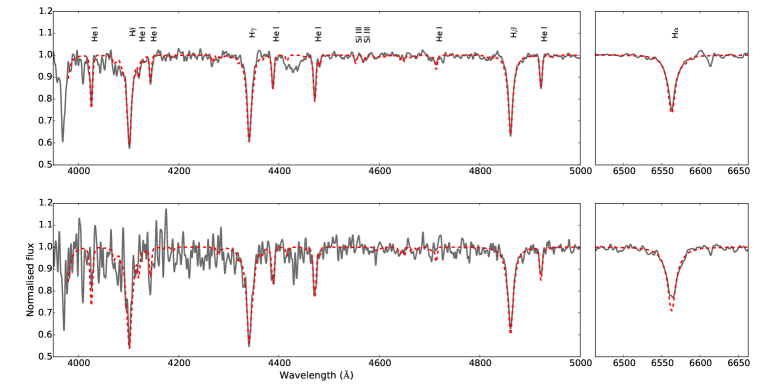
Figure 4: Normalized spectra of stars 1 and 2 observed with Gemini-South (plotted respectively in the upper and lower panels), compared with the best-fitting fastwind model (red dashed line). The lines fitted by the model are labelled.

To classify stars 1 and 2, we used their GMOS spectra. The spectra are dominated by H and He i absorption lines (see Fig. 4). No He ii lines are visible in the spectra, which implies that both stars are of B type. Using the EW(H$\gamma$)–absolute magnitude calibration by Balona & Crampton (1974) and the measured equivalent widths of EW(H$\gamma$)=4.5$\pm$0.1 Å  and 6.3$\pm$0.4 Å  for stars 1 and 2, respectively, we estimated their spectral types as B1 V and B3 V. The apparent luminosity resulting from the B1 V classification of star 1 is consistent with the location of IRAS 18153$-$1651 at the distance of 2 kpc (cf. Povich et al. 2016). We note that asymmetric profiles of the He i lines in the spectrum of star 2 suggest that this star might be a binary system. Nonetheless, the low spectral resolution and signal-to-noise ratio did not allow us to confirm this.

We modelled the spectra using the approach described in Castro et al. (2012; see also Lefever et al. 2010). The technique is rooted in a previously calculated fastwind (Santolaya-Rey, Puls & Herrero 1997; Puls et al. 2005) stellar atmosphere grid (e.g. Simon-Diaz et al. 2011; Castro et al. 2012) and a $\chi^{2}$-based algorithm, searching for the best set of parameters that reproduce the main strong optical lines observed between $\approx$4000$-$5000 Å  (labelled in Fig. 4). With the best-fitting models for stars 1 and 2 (see Fig. 4), we derived effective temperatures of $T_{\rm eff}$=22 000$\pm$2 000 K and 20 000$\pm$2 000 K, and surface gravities of $\log g$=4.2$\pm$0.2 and 4.4$\pm$0.2, respectively.

Main-sequence stars of these effective temperatures are sources of radiatively driven winds, which are strong enough to appreciably modify the ambient medium. In Table 2 we give mass-loss rates, $\dot{M}$, and terminal wind velocities, $v_{\infty}$, predicted by Krtička (2014) for main-sequence B stars with $T_{\rm eff}$ in the range of temperatures derived for stars 1 and 2, i.e. for $T_{\rm eff}\in[18\,000,24\,000]$ K. In this table we also give the rates of Lyman and dissociating Lyman-Werner photons (respectively, $Q_{0}$ and $Q_{\rm FUV}$) for the same range of effective temperatures (taken from Diaz-Miller, Franco & Shore 1998). The spectral classification of stars 1 and 2 implies that $T_{\rm eff}$ of star 1 should be at the upper end of the temperature range derived from spectral modelling, while that of star 2 – at the lower end (cf. Kenyon & Hartmann 1995). In the following, we adopt for these stars the effective temperatures of 24 and 18 kK, respectively. From Table 2 it then follows that the mechanical wind luminosity, $L_{\rm w}=\dot{M}v_{\infty}^{2}/2$, and radiation fluxes of star 1 are more than two orders of magnitude higher then those of star 2, so that we will consider the former star as the main energy source in IRAS 18153$-$1651.

Table 2: Mass-loss rates and terminal wind velocities of main-sequence B stars of solar metallicity and different effective temperatures as predicted by Krtička (2014), and rates of Lyman ($Q_{0}$) and dissociating Lyman-Werner ($Q_{\rm FUV}$) photons from Diaz-Miller et al. (1998).

$T_{\rm eff}$	$\dot{M}$	$v_{\infty}$	$Q_{0}$	$Q_{\rm FUV}$
(kK)	($\rm\,M_{\odot}\,{\rm yr}^{-1}$)	(${\rm\,km\,s^{-1}}$)	(${\rm s}^{-1}$)	(${\rm s}^{-1}$)
18	$9.1\times 10^{-12}$	820	$1.86\times 10^{43}$	$2.04\times 10^{46}$
20	$3.4\times 10^{-11}$	1 290	$1.35\times 10^{44}$	$6.03\times 10^{46}$
22	$7.9\times 10^{-11}$	1 690	$6.31\times 10^{44}$	$1.38\times 10^{47}$
24	$3.9\times 10^{-10}$	1 700	$2.40\times 10^{45}$	$2.45\times 10^{47}$

5 Optical arc

The GMOS slit was oriented along stars 1 and 2 and therefore it does not cross the optical arc. Correspondingly, we did not detect any signatures of nebular emission in the 2D spectrum. On the contrary, the slit of the TWIN spectrograph was oriented in such a way that it intersects the region of maximum brightness of the arc. Below we discuss the spectrum of the arc obtained with this spectrograph.

In the TWIN 2D spectrum the arc becomes visible via its emission lines of H$\alpha$, H$\beta$, [N ii] $\lambda\lambda$6548, 6584 and [S ii] $\lambda\lambda$6717, 6731 superimposed on strong continuum emission, which extends to the west of stars 1 and 2 for about 20 arcsec (see also Fig. 7). A part of this spectrum is presented in Fig. 5. Such composed spectra are typical of ionized reflection nebulae like the Orion Nebula (see e.g. plate XXIX in Greenstein & Henyey 1939). Correspondingly, we attribute the continuum emission to the starlight scattered by dust in the shell around the H ii  region.

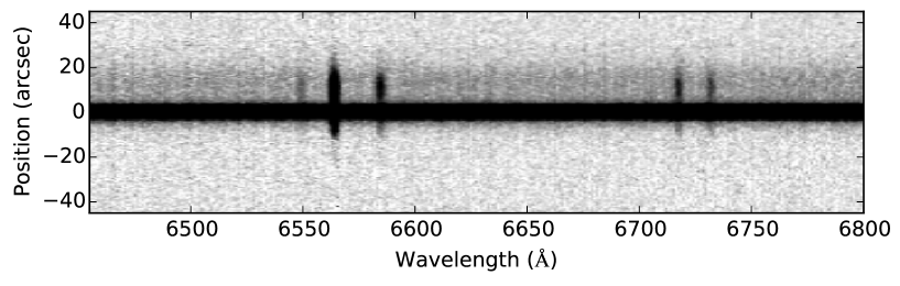
Figure 5: A part of the TWIN 2D spectrum of the optical emission around stars 1 and 2, showing nebular emission lines (from left to right) of [N ii] $\lambda$6548, H$\alpha$, [N ii] $\lambda$6584 and [S ii] $\lambda\lambda$6717, 6731. The upper part of the spectrum corresponds to the emission west of the stars. Note the presence of a strong continuum emission in this direction.

We extracted a 1D spectrum over the optical arc by summing up, without any weighting, all rows from the area of an annulus with an outer radius of 20 arcsec centred on stars 1 and 2 and the central $\pm$3 arcsec excluded. The resulting spectrum is presented in Fig. 6. The emission lines detected in the spectrum were measured using the programs described in Kniazev et al. (2004). Table 3 lists the observed intensities of these lines normalized to H$\beta$, $F$($\lambda$)/$F$(H$\beta$), the reddening-corrected line intensity ratios, $I$($\lambda$)/$I$(H$\beta$), and the logarithmic extinction coefficient, $C$(H$\beta$), which corresponds to a colour excess of $E(B-V)$=2.08$\pm$0.23 mag. In Table 3 we also give the electron number density derived from the intensity ratio of the [S ii] $\lambda\lambda$6716, 6731 lines, $n_{\rm e}$([S ii]). Both $C$(H$\beta$) and $n_{\rm e}$([S ii]) were calculated under the assumption that $T_{\rm e}=6\,500$ K (see Section 6.1). All calculations were done in the way described in detail in Kniazev et al. (2008).

Table 3: Line intensities in the Calar Alto spectrum of the optical arc.

$\lambda_{0}$(Å) Ion	$F$($\lambda$)/$F$(H$\beta$)	$I$($\lambda$)/$I$(H$\beta$)
4861 H$\beta$	1.00$\pm$0.37	1.00$\pm$0.39
6548 [N ii]	2.28$\pm$0.64	0.22$\pm$0.07
6563 H$\alpha$	31.21$\pm$8.12	2.94$\pm$0.87
6584 [N ii]	9.07$\pm$2.38	0.83$\pm$0.25
6716 [S ii]	6.07$\pm$1.59	0.48$\pm$0.07
6731 [S ii]	4.23$\pm$1.11	0.33$\pm$0.05
$C$(H$\beta$)	3.06$\pm$0.34
$E(B$$-$$V$)	2.08$\pm$0.23 mag
$n_{\rm e}$([S ii ])	10${}^{+550}_{-10}$ cm-3

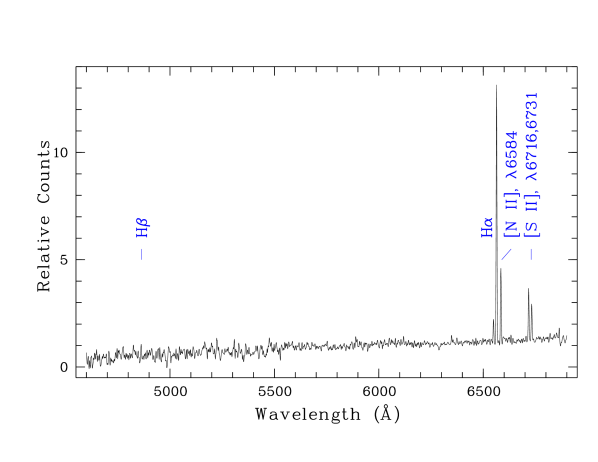
Figure 6: 1D spectrum of the optical arc obtained with the TWIN spectrograph.

The upper and middle panels in Fig. 7 plot, respectively, the H$\alpha$ line and continuum intensities and the H$\alpha$ heliocentric radial velocity distribution along the slit. A comparison of these panels with the SHS and MIPS images of IRAS 18153$-$1651 (presented for convenience in the bottom panel of Fig. 7) shows that in the west direction from stars 1 and 2 the H$\alpha$ and continuum emission extend to the edge of the mid-infrared nebula, and that the H$\alpha$ intensity peaks at the position of the arc. In the opposite direction, the H$\alpha$ line intensity is prominent up to a distance comparable to the radius of the arc, while the continuum emission fades at a shorter distance. From the lower panel of Fig. 7, we derived the mean heliocentric radial velocity of the H$\alpha$ emission of $31\pm 5\,{\rm\,km\,s^{-1}}$. Using this velocity and assuming the distance to the Galactic Centre of $R_{0}$=8.0 kpc and the circular rotation speed of the Galaxy of $\Theta_{0}=240\,{\rm\,km\,s^{-1}}$ (Reid et al. 2009), and the solar peculiar motion $(U_{\odot},V_{\odot},W_{\odot})=(11.1,12.2,7.3)\,{\rm\,km\,s^{-1}}$ (Schönrich, Binney & Dehnen 2010), one finds the local standard of rest velocity of $27\pm 5\,{\rm\,km\,s^{-1}}$, which agrees well with that of the cloud G14.225-0.506 (Jaffe et al. 1982; Busquet et al. 2013) and the star-forming region M17 SWex as a whole (e.g. Povich et al. 2016).

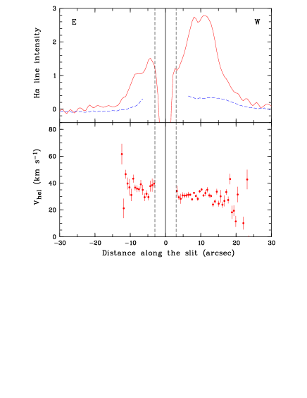
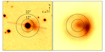
Figure 7: Upper panel: H$\alpha$ line and continuum emission intensities along the TWIN slit (PA=80$\degr$), shown respectively with a solid (red) and dashed (blue) lines. Middle panel: H$\alpha$ heliocentric radial velocity distribution along the slit. The E–W direction of the slit is shown. The solid vertical line corresponds to the position of star 1, while the dashed vertical lines (at $\pm$3 arcsec from the solid one) mark the area where the radial velocity was not measured because of the effect of stars 1 and 2. Bottom panel: SHS H$\alpha$+[N ii] (left) and MIPS $24\,\mu$m (right) images of IRAS 18153$-$1651 with the position of the TWIN slit shown by a red dashed rectangle. Concentric circles of radii 12 and 22 arcsec are overplotted on the images to make their comparison with the upper panels more convenient.

The electron number density could also be derived from the surface brightness of the arc in the H$\alpha$ line, $S_{{\rm H}\alpha}$, measured on the SHS image (cf. equation 4 in Frew et al. 2014):

$$n_{\rm e}\approx 1.7\,{\rm cm}^{-3}\left({l\over 1\,{\rm pc}}\right)^{-0.5}\left({T_{\rm e}\over 10^{4}\,{\rm K}}\right)^{0.45}$$

$$\times\left({S_{{\rm H}\alpha}\over 1\,{\rm R}}\right)^{0.5}e^{1.1E(B-V)}\,,$$ (1)

where $l$ is the line-of-sight thickness of the arc and 1 R$\equiv$1 Rayleigh=5.66$\times 10^{-18}$ erg cm^-2 s^-1 arcsec^-2 at H$\alpha$ (here we assumed that $n_{\rm e}$ and $T_{\rm e}$ are constant within the arc).

Using equations (1) and (2) in Frew et al. (2014) and the flux calibration factor of 20.4 counts pixel^-1 R^-1 from their table 1, and adopting the observed [N ii] to H$\alpha$ line intensity ratio of $0.36^{+0.30}_{-0.17}$ from Table 3 (here [N ii] corresponds to the sum of the $\lambda$6548 and $\lambda$6584 lines), we obtained the peak surface brightness of the arc (corrected for the contribution from the contaminant [N ii] lines) of $S_{{\rm H}\alpha}\approx$30${}^{+3}_{-4}$ R. Then, using equation (1) with $E(B-V)$=2.08$\pm$0.23 mag, $l$$\approx$0.23 pc (we assumed that the arc is a part of a spherical shell of inner radius of 12 arcsec and thickness of 5 arcsec) and $T_{\rm e}$=6 500 K (see Section 6.1), one finds $n_{\rm e}$$\approx$160${}^{+45}_{-35}$   ${\rm cm}^{-3}$, which agrees within the error margins with $n_{\rm e}$([S ii]) given in Table 3.

To find the actual H$\alpha$ surface brightness of the optical arc, $S_{{\rm H}\alpha}^{\rm act}$, one needs to estimate the attenuation of the H$\alpha$ emission line in magnitudes, $A$(H$\alpha$), in the direction towards IRAS 18153$-$1651, which is related to the visual extinction, $A_{V}=R_{V}E(B-V)$, through the following relationship: $A$(H$\alpha$)=$0.828A_{V}$ (e.g. James et al. 2005). Assuming a ratio of total to selective extinction of $R_{V}=3.1$ and using $E(B-V)$ from Table 3, one finds $A$(H$\alpha$)=5.34$\pm$0.59 mag and $S_{{\rm H}\alpha}^{\rm act}\approx 4\,100^{+3\,700}_{-2\,100}$ R.

Emission-line objects can be classified by using various diagnostic diagrams (see e.g. Kniazev, Pustilnik & Zucker 2008; Frew & Parker 2010, and references therein), of which the most frequently used one is $\log$(H$\alpha$/([S ii] $\lambda\lambda$6716, 6731)) versus $\log$(H$\alpha$/([N ii] $\lambda\lambda$6548, 6584)). For the optical arc one has $0.56^{+0.18}_{-0.20}$ versus 0.45$\pm$0.27 (see Table 3). These values place the arc in the area occupied by H ii  regions, although the large error bars allow the possibility that the arc is located within the domain occupied by supernova remnants, which means that the emission of the arc might be due to shock excitation.

Proceeding from this, one can suppose that the arc is either the edge of an asymmetric stellar wind bubble, distorted by a density gradient and/or stellar motion (e.g. Mackey et al. 2015, 2016), or a bow shock if the relative velocity between the wind-blowing star and the ambient medium is higher than the sound speed of the latter. The detection of two early type B stars separated from each other by only $\approx$2.3 arcsec (or 0.02 pc in projection) and the presence of a concentration of X-ray sources around them (see Section 2) suggest that we deal with a recently formed star cluster with stars 1 and 2 being its most massive members (cf. Gvaramadze et al. 2014b). This, in turn, implies that the mass of the cluster is about $100\,\rm\,M_{\odot}$ (e.g. Kroupa et al. 2013). We hypothesize therefore that the arc is the edge of the wind bubble blown by the wind of star 1 and suggest that the one-sided appearance of the bubble is caused by the interaction between the bubble and a photoevaporated flow from the molecular cloud to the west of the star (see Section 2).

Further, we interpret the more extended (mid-infrared) nebula around the arc as an H ii  region, so that the radius of the nebula is equal to the Strömgren radius $R_{\rm S}$. Proceeding from this, one can estimate the electron number density of the ambient medium:

$$n_{\rm e}=\sqrt{{3Q_{0}\over 4\pi\alpha_{\rm B}R_{\rm S}^{3}}}\,,$$ (2)

where $\alpha_{\rm B}=3.4\times 10^{-10}T^{-0.78}$ is the Case B recombination coefficient (Hummer 1994). This assumes that the electron and H⁺ number densities are the same, which is true for B stars because they cannot ionize helium. If $T$=6 500 K (see Section 6.1) and assuming $Q_{0}=2.4\times 10^{45}\,{\rm s}^{-1}$ (see Table 2), one finds from equation (2) that $n_{\rm e}\sim 100\,{\rm cm}^{-3}$.

In such a dense medium the bubble created by the wind of star 1 will soon become radiative (i.e. the radiative losses of the shocked wind material at the interface with the ISM become comparable to $L_{\rm w}$; cf. Mackey et al. 2015). This happens at the moment (McCray 1983):

$$t_{\rm rad}=1.5\times 10^{4}L_{33}^{0.3}n_{100}^{-0.7}\,{\rm yr}\,,$$ (3)

when the radius of the bubble is

$$R_{\rm rad}=0.2L_{33}^{0.4}n_{100}^{-0.6}\,{\rm pc}\,,$$ (4)

where $L_{33}=L_{\rm w}/(10^{33}\,{\rm erg}\,{\rm s}^{-1})$ and $n_{100}=n/(100\,{\rm cm}^{-3})$. Subsequent evolution of the bubble follows the momentum-driven solution by Steigman et al. (1975) and its radius is given by:

$$R(t)=R_{\rm rad}(t/t_{\rm rad})^{1/2}\,.$$ (5)

With $\dot{M}=3.9\times 10^{-10}\,\rm\,M_{\odot}\,{\rm yr}^{-1}$ and $v_{\infty}=1700\,{\rm\,km\,s^{-1}}$ (see Table 2), assuming $n=200\,{\rm cm}^{-3}$ (see Section 6.1), and using equations (3) and (4), one finds that $L_{\rm w}\approx 3.6\times 10^{32}\,{\rm erg}\,{\rm s}^{-1}$, $t_{\rm rad}\approx 7\,000$ yr and $R_{\rm rad}\approx 0.09$ pc. Then, it can be seen from equation (5) that the radius of the bubble would be equal to the observed radius of the optical arc of $\approx$0.11 pc if the bubble was formed only $\approx 11\,000$ yr ago. This inference is supported by numerical modelling presented in the next section.

6 Numerical Modelling

6.1 Simulations

To support our scenario for the origin of the optical arc, we ran 2D axisymmetric simulations using the pion code (Mackey & Lim 2010; Mackey 2012). The calculations solve the Euler equations of hydrodynamics and are accurate to second order in space and time. In addition, the non-equilibrium ionization fraction of hydrogen and heating and cooling processes are also calculated, mediated by the ionizing (EUV) and non-ionizing UV (FUV) radiation field that is calculated by a raytracing scheme. A uniform grid was used with cylindrical coordinates $z\in[-0.512,0.512]$ pc and $R\in[0,0.512]$ pc resolved by 1536 and 768 grid zones, respectively, for a grid resolution of $5\times 10^{-4}$ pc. Rotational symmetry around $R=0$ is assumed, and the simulations used the same general setup as Mackey et al. (2015).

We consider a single stellar source (a B1 star), with $T_{\rm eff}=24$ kK, using the wind and radiation properties in Table 2: $\dot{M}=4\times 10^{-10}\rm\,M_{\odot}\,{\rm yr}^{-1}$, $v_{\infty}=1700\,{\rm\,km\,s^{-1}}$, $Q_{0}=2.40\times 10^{45}$ s^-1 and $Q_{\rm FUV}=2.45\times 10^{47}$ s^-1. The FUV radiation heats the neutral gas around the star through photoelectric heating on grains, following the implementation of Henney et al. (2009). A uniform ISM was set up around the star with a H number density of $n_{\rm H}$=100, 200 and 300 cm^-3. In the following, however, we present only the results of simulations with $n_{\rm H}$=200 cm^-3 (or a mass density of $\rho=4.68\times 10^{-22}$g cm^-3) because they better match the observations. At $z>0.1$ pc the ISM was set to be 5 times denser, to mimic the nearby molecular cloud (although the real structure of the cloud must be more complicated, with substructure and density gradients; see Section 2 and Fig. 2). The gas is initially at rest and in pressure equilibrium, with $p/k_{\rm B}=1.1\times 10^{4}\,$K cm^-3, where $p$ is the gas pressure and $k_{\rm B}$ is the Boltzmann constant.

The evolution of this simulation is now described. The H ii  region expands rapidly in a spherical manner until it reaches the density jump at $z=0.1$ pc. At this interface a shock is transmitted into the dense medium and a second shock is reflected back into the H ii  region. This reflected flow subsequently develops into a photoevaporation flow from the dense medium. The equilibrium temperature of the H ii  region is $T\approx 6500$ K because of the very soft spectrum of the B1 star. The stellar wind drives a hot, expanding bubble within the H ii  region that is initially spherical. Subsequently this bubble is impacted by the trans-sonic flow from the dense medium through the H ii  region and is deformed. This creates a compressed and overpressurised layer between the dense molecular cloud and wind bubble. The ISM displaced by the wind bubble also creates an overdense layer in all directions at the interface between wind bubble and H ii  region. These two overdense regions are the brightest emitters in H$\alpha$. A snapshot from this simulation is shown in Fig. 8, where gas density and temperature are plotted on logarithmic scales.

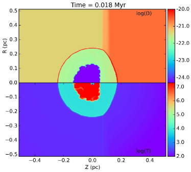
Figure 8: Gas density (upper half-plane) and temperature (lower half-plane) for the 2D simulation of the wind bubble and H ii  region described in the text, after 0.018 Myr of evolution. The units of density are $\log(\rho/{\rm g}\,{\rm cm}^{-3})$ and of temperature are $\log(T/{\rm K})$. This plot shows the simulated 2D plane, i.e., not projected onto the plane of the sky.

6.2 Synthetic maps and comparison with observations

Infrared emission from dust is calculated by postprocessing snapshots from the simulation using the torus code (Harris 2000, 2015; Kurosawa et al. 2015) following the method described in Mackey et al. (2016). A very similar approach using torus has also been used to model bow shocks around O stars (Acreman, Stevens & Harries 2016). Briefly, we use torus as a Monte-Carlo radiative transfer code to calculate the radiative equilibrium temperature of dust grains throughout the simulation, assuming radiative heating by the central star. The dust-to-gas ratio is assumed to be 0.01 in the ISM material (Draine et al. 2007), and we use a Mathis, Rumpl & Nordsieck (1977) grain-size distribution defined by the minimum (maximum) grain size $a_{\rm min}=0.005\,\mu$m ($a_{\rm max}=0.25\,\mu$m) and a power law index $q=3.3$. The calculations here are for spherical silicate grains (Draine & Lee 1984). torus calculates the dust temperature at all positions and then produces synthetic emission maps at different wavelengths from arbitrary viewing angles. Emission maps at 24 $\mu$m are shown in Fig. 9 for 5 different viewing angles, and the observational image from Spitzer is shown on the same scale for comparison. The projection where the line-of-sight is at 60$\degr$ to the symmetry axis of the simulation provides a reasonable match to the observations, both in terms of morphology and absolute brightness. The exception is that the observational image seems to have emission from the position of the star itself, absent from our models.

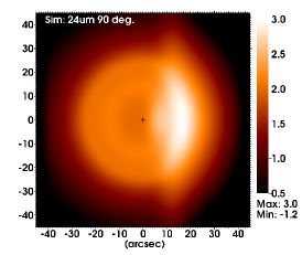
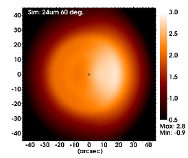
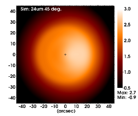
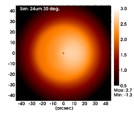
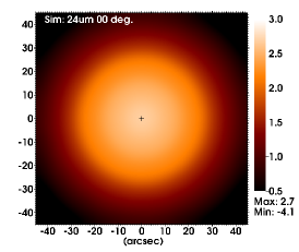
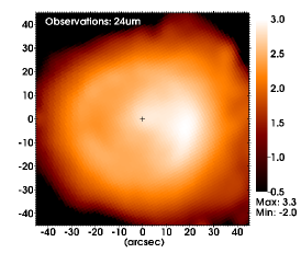
Figure 9: Synthetic dust emission maps at 24 $\mu$m of the simulated wind bubble and H ii  region, calculated by torus for Draine silicates. The panels show projections with a line-of-sight at angles of 90$\degr$, 60$\degr$, 45$\degr$, 30$\degr$, and 0$\degr$ to the symmetry axis of the simulation (left to right, top to bottom). The observational data are shown in the bottom right panel. The colour bar shows intensity at 24 $\mu$m on a log scale: $\log(I_{24\mu{\rm m}}/[{\rm MJy}\,{\rm ster}^{-1}])$. Synthetic images are smoothed to an angular resolution of the MIPS instrument of 6 arcsec (FWHM). A cross at the origin shows the location of the B1 star.

We also calculated H$\alpha$ emission from the simulation at a projection angle of 60$\degr$, because this angle was the best match to the 24 $\mu$m data. We did this using visit (Childs et al. 2012) and, while the relative brightness of each pixel is correctly calculated, there may be some scaling offset in the overall normalization of the image, so the absolute brightness should be treated with caution. The result is plotted in Fig. 10, where the left-hand panel shows the emission map over the full range of brightnesses and the right-hand one shows only the brightest 10 per cent of the predicted emission, to mimic the case where the brightest emission is just above the noise level (see Section 5). The brightest part of the simulated H$\alpha$ nebula is located within the H ii  region, about 10–15 arcsec from the star and well within the infrared bubble. This agrees very well with the observations in Fig. 1. Furthermore, Fig. 7 shows that the arc is about a factor of 2 brighter than the rest of the H ii  region in H$\alpha$ emission, comparable to what is shown in the left panel of Fig. 10.

Taken together, the agreement of the synthetic infrared and optical emission maps with the observational data is very encouraging. In particular, it suggests that H$\alpha$ imaging that is a factor of a few deeper would give a much clearer picture of the structure of this nebula, and strongly test our assertion that we are seeing a wind bubble and H ii  region from a main-sequence B star. The simulation setup is very simple, with little fine-tuning to match the observations. If further observations support the interpretation as a young stellar wind bubble, then more detailed 3D simulations including a clumpy or turbulent medium and a more realistic density structure of the molecular cloud would be clearly warranted. Particularly, one can expect that the presence of the denser material to the north-west of IRAS 18153$-$1651 (hub–N) would result in a stronger photoevaporation flow from this direction, which would explain the observed offset of stars 1 and 2 from the geometric centre of the mid-infrared bubble as well as from that of the optical arc (cf. Ngoumou et al. 2013).

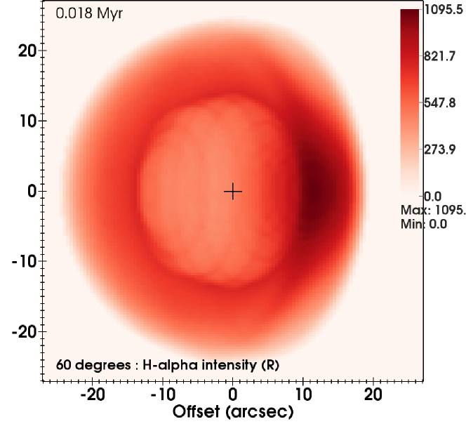
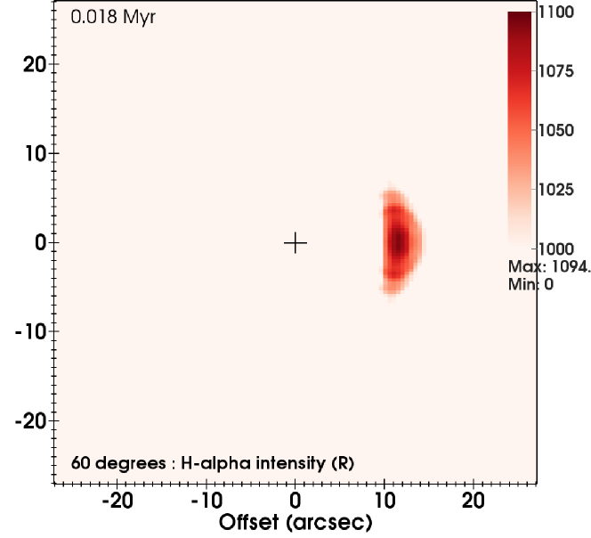
Figure 10: H$\alpha$ emission maps calculated with visit, for an angle of 60$\degr$ to the symmetry axis of the simulation. The upper panel shows the predicted H$\alpha$ surface brightness in R on a linear scale (although the absolute brightness should be treated with caution). The bottom panel shows only the brightest 10 per cent of the predicted emission, to mimic the case where the brightest emission is just above the noise level. A cross at the origin shows the location of the B1 star.

7 Summary and conclusion

In this paper, we have reported the study of a compact, almost circular mid-infrared nebula associated with the IRAS source 18153$-$1651 and located in the region of ongoing massive star formation M17 SWex. The study was motivated by the discovery of an optical arc near the centre of the nebula, leading to the hypothesis that it might represent a bubble blown by the wind of a young massive star. To substantiate this hypothesis, we obtained optical spectra of the arc and two stars near its focus with the Gemini-South and the 3.5-m telescope in the Observatory of Calar Alto (Spain). The stars have been classified as main-sequence stars of spectral type B1 and B3, while the line ratios in the spectrum of the arc indicated that its emission is due to photoionization $<...>$. These findings allowed us to suggest that we deal with a recently formed low-mass ($\sim 100\,\rm\,M_{\odot}$) star cluster (with the two B stars being its most massive members) and that the optical arc and IRAS 18153$-$1651 are, respectively, the edge of a wind bubble and the H ii  region produced by the B1 star. We also suggested that the one-sided appearance of the wind bubble is the result of interaction between the bubble and a photoevaporation flow from a molecular cloud located to the west of IRAS 18153$-$1651 (the presence of such a cloud is evidenced by submillimetre and radio observations). We supported our suggestions by simple analytical estimates, showing that the radii of the bubble and the H ii  region would fit the observations if the age of IRAS 18153$-$1651 is $\sim 10\,000$ yr and the number density of the ambient medium is $\sim 100\,{\rm cm}^{-3}$. These estimates were validated by two-dimensional, radiation-hydrodynamics simulations investigating the effect of a nearby dense cloud on the appearance of newly forming wind bubble and H ii  region. We found that synthetic H$\alpha$ and 24 $\mu$m dust emission maps of our model wind bubble and H ii  region show a good match to the observations, both in terms of morphology and surface brightness.

To conclude, taken together our results strongly suggest that we have revealed the first example of a wind bubble blown by a main-sequence B star.

8 Acknowledgements

VVG acknowledges the Russian Science Foundation grant 14-12-01096. JM acknowledges funding from a Royal Society–Science Foundation Ireland University Research Fellowship (No. 14/RS-URF/3219). AYK acknowledges support from the National Research Foundation (NRF) of South Africa and the Russian Foundation for Basic Research grant 16-02-00148. TJH is funded by an Imperial College Junior Research Fellowship. This research was supported by the Gemini Observatory, which is operated by the Association of Universities for Research in Astronomy, Inc., on behalf of the international Gemini partnership of Argentina, Brazil, Canada, Chile, and the United States of America, and has made use of the NASA/IPAC Infrared Science Archive, which is operated by the Jet Propulsion Laboratory, California Institute of Technology, under contract with the National Aeronautics and Space Administration, the SIMBAD data base and the VizieR catalogue access tool, both operated at CDS, Strasbourg, France.

References

- (1) Acreman D. M., Stevens I. R., Harries T.J., 2016, MNRAS, 456, 136
- (2) Balona L., Crampton D., 1974, MNRAS, 166, 203
- (3) Benjamin R. A. et al., 2003, PASP, 115, 953
- (4) Blaauw A., 1961, Bull. Astron. Inst. Netherlands, 15, 265
- (5) Busquet G. et al., 2013, ApJ, 764, L26
- (6) Busquet G. et al., 2016, ApJ, 819, 139
- (7) Carey S. J. et al., 2009, PASP, 121, 76
- (8) Castro N. et al., 2012, A&A, 542, A79
- (9) Childs H. et al., 2012, in Hansen C., Childs H., Bethel E., eds., High Performance Visualization: Enabling Extreme-Scale Scientific Insight. Chapman and Hall/CRC, p. 357
- (10) Christopoulou P. E., Goudis C. D., Meaburn J., Dyson J. E., Clayton C. A., 1995, A&A, 295, 509
- (11) Chu Y.-H., Treffers R. R., Kwitter K. B., 1983, ApJS, 53, 937
- (12) Courtes G., Petit H., Petit M., Sivan J.-P., Dodonov S., 1987, A&A, 174, 28
- (13) Davies R. D., Elliott K. H., Meaburn J., 1976, MmRAS, 81, 89
- (14) Diaz-Miller R. I., Franco J., Shore S. N., 1998, ApJ, 501, 192
- (15) Dopita M. A., Bell J. F., Chu Y.-H., Lozinskaya T. A., 1994, ApJS, 93, 455
- (16) Draine B. T., Lee H. M., 1984, ApJ, 285, 89
- (17) Draine B. T. et al., 2007, ApJ, 663, 866
- (18) Eldridge J. J., Langer N., Tout C. A., 2011, MNRAS, 414, 3501
- (19) Fazio G. G. et al., 2004, ApJS, 154, 10
- (20) Frew D. J., Parker Q. A., 2010, PASA, 27, 129
- (21) Frew D. J., Bojičić I. S., Parker Q. A., Pierce M. J., Gunawardhana M. L. P., Reid W. A., 2014, MNRAS, 440, 1080
- (22) Gies D.R,. 1987, ApJS, 64, 545
- (23) Greenstein J. L., Henyey L. G., 1939, ApJ, 89, 647
- (24) Gvaramadze V. V., Bomans D. J., 2008, A&A, 490, 1071
- (25) Gvaramadze V. V., Weidner C., Kroupa P., Pflamm-Altenburg J., 2012, MNRAS, 424, 3037
- (26) Gvaramadze V. V., Menten K. M., Kniazev A. Y., Langer N., Mackey J., Kraus A., Meyer D. M.-A., Kaminski T., 2014a, MNRAS, 437, 843
- (27) Gvaramadze V. V. et al., 2009, MNRAS, 400, 524
- (28) Gvaramadze V. V. et al., 2014b, MNRAS, 442, 929
- (29) Jaffe D. T., Güsten R., Downes D., 1981, ApJ, 250, 621
- (30) Jaffe D. T., Stier M. T., Fazio G. G., 1982, ApJ, 252, 601
- (31) James P. A., Shane N. S., Knapen J. H., Etherton J., Percival S. M., 2005, A&A, 429, 851
- (32) Johnson H. M., Hogg D. E., 1965, ApJ, 142, 1033
- (33) Harries T. J., 2000, MNRAS, 315, 722
- (34) Harries T. J., 2015, MNRAS, 448, 3156
- (35) Henden A. A, Templeton M., Smith T. C., Levine S., Welch D., 2016, VizieR Online Data Catalog, 2336, 0
- (36) Henney W. J., Arthur S. J., de Colle F., Mellema G., 2009, MNRAS, 398, 157
- (37) Hummer D. G., 1994, MNRAS, 268, 109
- (38) Hunter D. A., 1994, AJ, 108, 1658
- (39) Kenyon S. J., Hartmann L., 1995, ApJS, 101, 117
- (40) Kniazev A. Y., Pustilnik S. A., Zucker D. B., 2008, MNRAS, 384, 1045
- (41) Kniazev A. Y., Pustilnik S. A., Grebel E. K., Lee H., Pramskij A. G., 2004, ApJS, 153, 429
- (42) Kniazev A. Y. et al., 2008, MNRAS, 388, 1667
- (43) Kroupa P., Weidner C., Pflamm-Altenburg J., Thies I., Dabringhausen J., Marks M., Maschberger T., 2011, in Oswalt T. D., Gilmore G., eds., Planets, Stars and Stellar Systems, Vol. 5. Springer Science+Business Media Dordrecht, p. 115
- (44) Krtička J., 2014, A&A, 564, A70
- (45) Kurosawa R., Harries T. J., Bate M. R., Symington N. H., 2004, MNRAS, 351, 1134
- (46) Lada C.J., Lada E.A., 2003, ARA&A, 41, 57
- (47) Lefever K., Puls J., Morel T., Aerts C., Decin L., Briquet M., 2010, A&A, 515, A74
- (48) Lucas P. W. et al., 2008, MNRAS, 391, 136
- (49) Lozinskaya T. A., Lomovskij A.I., 1982, Sov. Astron. Lett., 8, 119
- (50) Mackey J., 2012, A&A, 539, A147
- (51) Mackey J., Lim A. J., 2010, MNRAS, 403, 714
- (52) Mackey J., Gvaramadze V. V., Mohamed S., Langer N., 2015, A&A, 573, A10
- (53) Mackey J., Haworth T. J., Gvaramadze V. V., Mohamed S., Langer N., Harries, T. J., 2016, A&A, 586, A114
- (54) Mathis J. S., Rumpl W., Nordsieck K. H., 1977, ApJ, 217, 425
- (55) McCray R., 1983, Highlights Astron., 6, 565
- (56) McCray R., Kafatos M., 1987, ApJ, 317, 190
- (57) McLean B. J., Greene G. R., Lattanzi M. G., Pirenne B., 2000, in Manset N., Veillet C., Crabtree D., eds, ASP Conf. Ser. Vol. 216, Astronomical Data Analysis Software and Systems IX. Astron. Soc. Pac., San Francisco, p. 145
- (58) Meaburn J., 1980, MNRAS, 192, 365
- (59) Moore B. D., Walter D. K., Hester J. J., Scowen P. A., Dufour R. J., Buckalew B. A., 2002, AJ, 124, 3313
- (60) Nazé Y., Chu, Y.-H., Points S. D., Danforth C. W., Rosado M., Chen C.-H. R., 2001, AJ, 122, 921
- (61) Ngoumou J., Preibisch T., Ratzka T., Burkert, A. 2013, ApJ, 769, 139
- (62) Oh S, Kroupa P., 2016, A&A, 590, A107
- (63) Oke J. B., 1990, AJ, 99, 1621
- (64) Parker Q. A. et al., 2005, MNRAS, 362, 689
- (65) Peretto N., Fuller G. A., 2009, A&A, 505, 405
- (66) Poveda A., Ruiz J., Allen C., 1967, Bol. Obs. Tonantzintla Tacubaya, 4, 86
- (67) Povich M. S., Whitney, B. A., 2010, ApJ, 714, L285
- (68) Povich M. S., Townsley L. K., Robitaille T. P., Broos P. S., Orbin W. T., King R. R., Naylor T., Whitney B. A., 2016, ApJ, 825, 125
- (69) Puls J., Vink J., Najarro F., 2008, A&AR, 16, 209
- (70) Puls J., Urbaneja M. A., Venero R., Repolust T., Springmann U., Jokuthy A., Mokiem M. R., 2005, A&A, 435, 669
- (71) Reid M. J., Menten K. M., Zheng X. W., Brunthaler A., Xu Y., 2009, ApJ, 705, 1548
- (72) Rieke G. H. et al., 2004, ApJS, 154, 25
- (73) Santolaya-Rey A. E., Puls J., Herrero A., 1997, A&A, 323, 488
- (74) Santos F. P., Busquet G., Franco G. A. P., Girart J. M., Zhang Q., 2016, preprint (arXiv:1609.08052)
- (75) Schönrich R., Binney J., Dehnen W., 2010, MNRAS, 403, 1829
- (76) Schuller F. et al., 2009, A&A, 504, 415
- (77) Simón-Díaz S., Castro N., Herrero A., Puls J., Garcia M., Sabín-Sanjulián C., 2011, JPhCS, 328, 012021
- (78) Snow T. P., Morton D. C., 1976, ApJS, 32, 429
- (79) Sota A., Maíz Apellániz J., Walborn N. R., Alfaro E. J., Barbá R. H., Morrell N. I., Gamen R. C., Arias J. I., 2011, ApJS, 193, 24
- (80) Spitzer Science Center, 2009, VizieR Online Data Catalog, 2293, 0
- (81) Steigman G., Strittmatter P. A., Williams R. E., 1975, ApJ, 198, 575
- (82) van Buren, D., McCray, R. 1988, ApJ, 329, L93
- (83) Wang Y., Zhang Q., Rathborne J. M., Jackson J., Wu Y., 2006, ApJL, 651, L125
- (84) Weaver R., McCray R., Castor J., Shapiro P., Moore R., 1977, ApJ, 218, 377