YGHP-16-07

TIT/HEP-657

Dec., 2016

Thermal Inflation with Flaton Chemical Potential

Masato Arai, Yoshishige Kobayashi^†, Nobuchika Okada $\ddagger$ ,
and Shin Sasaki^#,
Faculty of Science, Yamagata University
Yamagata 990-8560, Japan
^†Department of Physics, Tokyo Institute of Technology
Tokyo 152-8551, Japan
^‡Department of Physics and Astronomy
University of Alabama, Tuscaloosa, AL35487, USA
^#Department of Physics, Kitasato University
Sagamihara 252-0373, Japan

Thermal inflation driven by a scalar field called “flaton” is a possible scenario to solve the cosmological moduli problem. We study a model of thermal inflation with a flaton chemical potential. In the presence of the chemical potential, a negative mass squared of the flaton, which is necessary to terminate the thermal inflation, is naturally induced. We identify the allowed parameter region for the chemical potential ($\mu$) and the flaton self-coupling constant to solve the cosmological moduli problem and satisfy theoretical consistencies. In general, the chemical potential is a free parameter and it can be taken to be much larger than the typical scale of soft supersymmetry breaking parameters of $\mathcal{O}(1)$ TeV. For $\mu\gtrsim 10^{8}$ GeV, we find that the reheating temperature after the thermal inflation can be high enough for the thermal leptogenesis scenario to be operative. This is in sharp contrast to the standard thermal inflation scenario, in which the reheating temperature is quite low and a special mechanism is necessary for generating sufficient amount of baryon asymmetry in the Universe after thermal inflation.

1 Introduction

The exponentially accelerated expansion of spacetime in the early period of the Universe is well-established as the cosmic inflation scenario [1, 2, 3, 4, 5]. The primordial inflation solves the flatness and the horizon problems in the Standard Big-Bang cosmology. On the other hand, supersymmetry (SUSY) is believed to play an important role in the study of elementary particles especially in the early stage of the Universe. It is known that the inflation scenarios in the supersymmetric epoch exhibit various problems. Among other things, the relatively high reheating temperature after the primordial inflation causes the overproduction of gravitino. Late time decay of gravitino after the Big-Bang Nucleosynthesis deconstruct successfully synthesized light elements. This is known as the gravitino problem [6, 7, 8]. One resolution to the gravitino problem is achieved by a low reheating temperature $T_{\rm RH}\lesssim 10^{6-7}$ GeV [9, 10].

There is also a serious cosmological problem in the early Universe, known as the cosmological moduli problem [11, 12, 13]. The four-dimensional spacetime may be realized in superstring theories, which typically predict massless scalar excitations, i.e., moduli fields. Since the moduli fields only have Planck suppressed interactions, the energy density of the Universe is dominated by the moduli fields before they decay. If the moduli decay cannot reheat the Universe high enough $T_{\rm RH}\gtrsim 1$ MeV, the present Universe cannot be realized. This is the cosmological moduli problem. This problem is intractable in the primordial inflation scenario since the moduli particles are produced abundantly even in the low reheating temperature.

In order to solve the moduli problem, a short period of the secondary inflation with $\mathcal{O}(10)$ e-foldings after the primordial inflation has been proposed [14, 15]. By this second inflation, the number density of the moduli particles is diluted away and their energy density never dominate the Universe. Since this secondary inflation of spacetime is triggered by the thermal effect, this is called the thermal inflation. Realization and phenomenological viability of the thermal inflation have been discussed in detail, for example, in [16, 17, 18, 19, 20, 21].

The thermal inflation is driven by a scalar field with an almost flat potential. This field is called flaton. The typical flaton potential at zero temperature is given by [15]

$$V(\phi)=V_{0}-m_{\phi 0}^{2}|\phi|^{2}+\sum_{n=1}^{\infty}\lambda_{n}{|\phi|^{2n+4}\over\bar{M}_{\text{pl}}^{2n}}\,,$$ (1)

where $\phi$ is the (complex scalar) flaton field, $V_{0}$ is the vacuum energy at the origin, $m_{\phi 0}$ is the mass of the flaton and $\lambda_{n}$ are the coupling constants. The higher dimensional interactions are suppressed by the reduced Planck mass $\bar{M}_{\text{pl}}=2.4\times 10^{18}$ GeV. Here the flaton is assumed to interact with a scalar field $X$ which serves as the thermal bath, through which the flaton potential $V$ receives finite temperature corrections from the thermal bath. At a high temperature $T$, the effective mass squared $m^{2}(T)$ of the flaton behaves like $m^{2}(T)=T^{2}-m_{\phi 0}^{2}>0$ and the thermal inflation begins at $\phi=0$. As the temperature decreases, the effective mass squared turns negative, which leads to the violation of the slow-roll condition. Therefore the tachyonic mass of the flaton is necessary for the end of the thermal inflation. It has been discussed that the tachyonic mass is obtained by the renormalization group flow in a supersymmetric model [22]. However, this does not happen in more general situations. After the thermal inflation, the flaton rolls down to the true vacuum and then starts to oscillate there. The flaton decays to the Standard Model particles to reheat the Universe. This decay creates entropy, and the moduli problem can be solved. In order to solve the moduli problem, the yield of the moduli field after the thermal inflation must be reduced to $10^{-12}-10^{-15}$ [23] or smaller. However, this mechanism causes another problem: the entropy production by the flaton decay also dilutes the primordial baryon asymmetry produced by some mechanism beforehand. We need a mechanism to produce sufficient amount of baryon asymmetry before or after the thermal inflation. In [16, 19, 21], it has been studied whether sufficient baryon number asymmetry is produced with the use of the Affleck-Dine mechanism [25, 26] after the thermal inflation. However, it was found that the Affleck-Dine mechanism is not phenomenologically viable in this framework. It is normally difficult to resolve the problem since the reheating temperature after the flaton decay is typically not high enough, because of very weak couplings of the flaton to the Standard Model particles.

In this paper we propose a thermal inflation scenario that can solve the problems of termination of the thermal inflation and of generating sufficient amount of baryon asymmetry after the flaton decay. For this purpose, we introduce a chemical potential $\mu$ for the flaton. We will show that in the thermal effective potential, the chemical potential $\mu$ plays a role of the tachyonic mass of the flaton at low temperature. Hence, the thermal inflation ends when the chemical potential starts dominating over the thermal mass. Furthermore, $\mu$ is a free parameter in any system, which basically has nothing to do with soft SUSY breaking parameters. This is in contrast with the standard thermal inflation scenario where the tachyonic mass term in (1) is supposed to be generated through SUSY breaking and hence we expect $|m_{\phi_{0}}|\simeq{\cal O}(1)$ TeV for the weak scale SUSY. The mass scale of the flaton is important since it determines the reheating temperature ($T_{\rm RH2}$) after the flaton decay and what mechanism for the baryon number generation can be implemented. In the standard thermal inflation scenario, $T_{\rm RH2}$ is at most ${\cal O}(100)$ MeV as we will discuss below. With such a low reheating temperature, a possible scenario for the baryon number generation is the Affleck-Dine mechanism [25, 26]. As mentioned above, although the Affleck-Dine mechanism has been studied in models of the thermal inflation, it turns out that sufficient amount of baryon number cannot be created [16, 19, 21]. In our model, we can set $\mu\gg 1$ TeV so that the reheating temperature can be much higher and the thermal leptogenesis [27] (for review, see [28]) can be operative even after the flaton decay.

The organization of this paper is as follows. In the next section, we present a brief review on the standard thermal inflation. In section 3, we introduce a chemical potential for the flaton field and calculate the thermal effective potential of the flaton. We then evaluate the yields of the moduli after the flaton decay and identify the allowed regions of the chemical potential $\mu$ and the flaton coupling constant $\lambda$. Section 4 is devoted to conclusions and discussions. We give a brief derivation of the thermal effective potential in Appendix A. In Appendix B, we derive the interaction term between the flaton and the Standard Model gauge fields.

2 Review of Standard Thermal Inflation

In this section, we review the thermal inflation proposed in [14, 15] and how the moduli problem is solved. If the flaton field causes thermal inflation, the energy density by the oscillating moduli is diluted and hence the moduli problem can be solved. After the thermal inflation, the Universe is thermalized with the reheating temperature $T_{\rm RH2}$ through the flaton decay. If the reheating temperature is high enough to allow the Big-Bang nucleosynthesis ($T_{\rm RH2}\gtrsim 1$ MeV), the history of the Universe becomes the standard scenario.

We focus on a part of a model which causes the thermal inflation while a part for the primordial inflation is not specified. We assume that the flaton field acquires its mass via SUSY breaking, and hence the mass is naturally of the order of the soft SUSY breaking mass scale $\sim 1$ TeV. Notice that as we will see below, the negative mass squared for the flaton field is necessary to terminate the thermal inflation. For an origin of the negative mass squared, we may consider the renormalization group effect, which drives the running flaton mass squared negative at a certain low scale. For a concrete model, see [22].

The flaton field $\phi$ is considered to couple with some light fields, typically the Standard Model particles, which are in thermal equilibrium and yield thermal corrections to the effective potential of the flaton. The high-temperature approximation is valid, when the mass scale of the fields are sufficiently small compared to the temperature during the thermal inflation. For simplicity, we consider a model, with two real scalars $\phi$ and $X$ for the thermal inflation,

$${\cal L}={1\over 2}\partial_{\mu}\phi\partial^{\mu}\phi+{1\over 2}\partial_{\mu}X\partial^{\mu}X-V(\phi,X)\,,$$ (2)

where $\mu=0,1,2,3$ is the spacetime index, and we use the mostly minus convention of the metric $\eta_{\mu\nu}={\rm diag}(1,-1,-1,-1)$. The scalar potential $V$ is given to be the following form

$$V_{\rm tree}=V_{0}-{m_{\phi 0}^{2}\over 2}\phi^{2}+{\lambda\over 6\bar{M}_{\rm pl}^{2}}\phi^{6}+{m_{X0}^{2}\over 2}X^{2}+{g\over 4}\phi^{2}X^{2}\,,$$ (3)

where $V_{0}$ is the energy scale at the origin, and $m_{\phi 0}$ and $m_{X0}$ are the masses of the fields $\phi$ and $X$, respectively. Here $\lambda$ and $g$ are coupling constants. We have introduced the higher dimensional interaction term $\phi^{6}$, and there is no flaton quartic term. This setting realizes an almost flat potential and leads to a large vacuum expectation value (VEV) of the flaton field. Such a large VEV is crucial to solve the moduli problem [15] (see, (30) with (6)). The stationary condition for $X$ trivially gives $X=0$ while the one for $\phi$,

$${\partial V\over\partial\phi}{\Big{|}}_{X=0}=0$$ (4)

yields

$$\phi=0,\qquad\phi=\lambda^{-1/4}\sqrt{m_{\phi 0}\bar{M}_{\rm pl}}\equiv M\,.$$ (5)

The energy scale at the origin is given by

$$V_{0}={1\over 3\sqrt{\lambda}}m_{\phi 0}^{3}\bar{M}_{\rm pl}={1\over 3}m_{\phi 0}^{2}M^{2},$$ (6)

which guarantees the vanishing cosmological constant at the potential minimum $\phi_{c}=M$. We represent $\phi_{c}$ as the VEV of $\phi$.

The scalar potential (3) receives thermal effects through the reheating after the primordial inflation. The thermal effects are introduced by imposing the periodic boundary condition for the fields $\Phi_{i}=(\phi,X)$ as $\Phi_{i}(\tau,\vec{x})=\Phi_{i}(\tau+\beta,\vec{x})$ in the partition function, where $\tau=ix_{0}$ is the imaginary time, $\beta=1/T$ is the inverse temperature and $\vec{x}=(x_{1},x_{2},x_{3})$. The partition function is given as

$$Z = {\rm Tr}e^{-\beta H}$$ (7)

$$= \int_{\Phi_{i}(\tau)=\Phi_{i}(\tau+\beta)}\prod_{i}{\cal D}\Phi_{i}{\cal D}\Phi_{i}^{\dagger}e^{-\int_{0}^{\beta}d\tau\int d^{3}x\sum_{i}({1\over 2}\partial_{0}\Phi_{i}\partial_{0}\Phi_{i}+{1\over 2}\vec{\nabla}\Phi_{i}\vec{\nabla}\Phi_{i}+V(\phi,X))}\,,$$

where $H$ is the Hamiltonian and $\vec{\nabla}$ is the derivative with respect to $\vec{x}$. The scalar field $X$ plays the role of the thermal bath and the flaton receives the thermal effects through $X$-loop corrections. Calculating the thermal 1-loop correction of $X$, we obtain the effective potential for the flaton as [30]

$$V_{\rm eff}(\phi_{c}) = V_{0}-{1\over 2}m_{\phi 0}^{2}\phi_{c}^{2}+{\lambda\over 6\bar{M}_{\rm pl}^{2}}\phi_{c}^{6}+\int{d^{3}k\over(2\pi)^{3}}{\omega_{k}\over 2}+{1\over\beta}\int{d^{3}k\over(2\pi)^{3}}\log\left(1-e^{-\beta\omega_{k}}\right)\,,$$ (8)

where we have defined

$$\omega_{k}^{2} = \vec{k}^{2}+m_{X}^{2}(\phi)\,,$$ (9)

$$m_{X}^{2}(\phi) = {\partial^{2}V\over\partial X^{2}}{\Big{|}}_{\phi=\phi_{c}}=m_{X0}^{2}+{1\over 2}g\phi_{c}^{2}\,.$$ (10)

The fourth term in the right hand side of (8) is the Coleman-Weinberg potential and the fifth term is the thermal effective potential. We consider the situation where the temperature is high enough and the dominant contribution comes from the thermal effective potential. In the subsequent discussions, we therefore neglect the Coleman-Weinberg potential term. Performing the high temperature expansion, we have

$$V_{\rm eff}(\phi_{c})=V_{0}-{\pi^{2}T^{4}\over 90}+{T^{2}\over 24}m_{X0}^{2}+{1\over 2}m_{\phi}^{2}(T)\phi_{c}^{2}+{\lambda\over 6\bar{M}_{\rm pl}^{2}}\phi_{c}^{6}+\cdots\,,$$ (11)

where $m_{\phi}(T)$ is the flaton mass with the thermal correction:

$$m_{\phi}(T)^{2}=-m_{\phi 0}^{2}+{g\over 24}T^{2}\,.$$ (12)

For $m_{\phi}(T)^{2}>0$, the vacuum is located at $\phi_{c}=0$, and the potential energy of the flaton dominates over the energy of the Universe. This leads to the second inflation by the flaton, namely, the thermal inflation. The thermal inflation ends when the effective mass of the flaton turns to be negative, in other words, when the temperature drops below the critical value $T_{C}$ given by

$$T_{C}=2m_{\phi 0}\sqrt{6\over g}\,.$$ (13)

Soon after the temperature becomes less than $T_{C}$, the flaton starts rolling down to the vacuum at $\phi_{c}=M$ and then oscillates around there. The decay of the flaton reheats the Universe, and we roughly estimate the reheating temperature as

$$T_{\rm RH2}\simeq\left(90\over\pi^{2}g_{*}\right)^{1/4}\sqrt{\Gamma\bar{M}_{\rm pl}}\,,$$ (14)

where $g_{*}(\simeq 200)$ counts the effective degrees of freedom of the radiation, and $\Gamma$ is the flaton decay width. Here we simply assume that the flaton decays to the Higgs boson ($h$) through the effective interaction [18]

$${\cal L}_{\rm int}\sim{m_{\phi}^{2}\over M}\phi hh\,,$$ (15)

where $m_{\phi}$ is the flaton mass in the vacuum at $T=0$ and given by

$$m_{\phi}^{2}={\partial^{2}V\over\partial\phi^{2}}{\Big{|}}_{T=0,\phi_{c}=M}=4m_{\phi 0}^{2}\,.$$ (16)

The decay width of the process $\phi\rightarrow hh$ is obtained as

$$\Gamma\simeq{1\over 16\pi}{m_{\phi}^{3}\over M^{2}}\,,$$ (17)

where we have neglected the Higgs boson mass. Substituting (17) into (14), we find the reheating temperature as

$$T_{\rm RH2}\simeq\left(90\over\pi^{2}g_{*}\right)^{1/4}{m_{\phi}\over 4M}\sqrt{m_{\phi}\bar{M}_{\rm pl}\over\pi}={1\over 4\pi}\left(360\lambda\over g_{*}\right)^{1\over 4}m_{\phi}\,.$$ (18)

The main role of the thermal inflation is to dilute the yield of the moduli field, by which the moduli problem is solved. The dilution is caused by the entropy production by the flaton decay after the thermal inflation. Before we discuss the entropy production, we note that there are two relevant scenarios for the moduli oscillation after the primordial inflation (see Fig. 1). The first is the one discussed in [15]. In this scenario, the moduli fields are displaced from the potential minima during the primordial inflation. When the Hubble parameter reduces to $H\sim m_{\Phi}$, the moduli fields start to oscillate around their potential minima. Here $m_{\Phi}$ is the mass of the moduli fields. The Universe enters the matter dominated era with the oscillating inflaton and moduli fields whose energy densities are comparable. After the moduli oscillation, the first reheating takes place by the decay of the inflaton and we denote the reheating temperature by $T_{\text{RH}1}$.

The second possibility is that the moduli oscillation takes place after the first reheating. When the Universe cools down to $H\sim m_{\Phi}$, the moduli fields start to oscillate. As we will see later, in both scenarios, the oscillating moduli, that dominate the energy density of the Universe, can be diluted away by the thermal inflation.

In the following, we make a qualitative analysis on the entropy production in these scenarios.

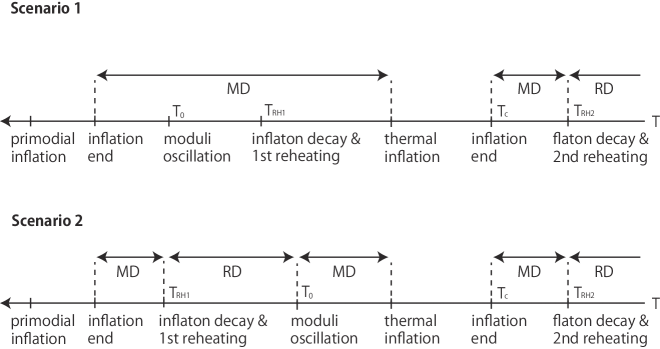
Figure 1: Two possible scenarios for the moduli oscillation in the thermal history of the Universe. Here MD and RD mean the matter dominant and the radiation dominant, respectively.

Scenario 1

The increase of the entropy density after the flaton decay is calculated as

$$\Delta={s(T_{\rm RH2})\over s(T_{C})}\,,$$ (19)

where $s(T)$ is the entropy density at temperature $T$. In the radiation dominated era, this is given by

$$s(T)={2\pi^{2}\over 45}g_{*}T^{3}={4\rho(T)\over 3T}\,,$$ (20)

where we have used the energy density for relativistic particles

$$\rho(T)={\pi^{2}\over 30}g_{*}T^{4}\,.$$ (21)

With the use of the relation (20), the increase of the entropy (19) is expressed as

$$\Delta={30V_{0}\over\pi^{2}g_{*}T_{C}^{3}T_{\rm RH2}}\,,$$ (22)

where we have used $V_{0}=\rho(T_{\rm RH2})$.

The yield of the moduli $Y_{\Phi}$ after the flaton decay is given by

$$Y_{\Phi}={n_{\Phi}(T_{\rm RH2})\over s(T_{\rm RH2})}={n_{\Phi}(T_{C})\over s(T_{C})\Delta}={n_{\Phi}(T_{\rm RH1})\over s(T_{\rm RH1})\Delta}\,,$$ (23)

where $n_{\Phi}$ is the number density of the moduli particles, and we have assumed no entropy production before the end of the thermal inflation. Since the moduli particles are non-relativistic in this era, $n_{\Phi}$ at a certain temperature is represented by

$$n_{\Phi}={1\over m_{\Phi}}\rho_{\Phi}\,,$$ (24)

where $\rho_{\Phi}$ is the energy density of the moduli. The energy density of the moduli at $T_{\rm RH2}$ is produced by moduli oscillation after the primordial inflation:

$$\rho_{\Phi}={1\over 2}m_{\Phi}^{2}\Phi_{0}^{2}\,,$$ (25)

where $\Phi_{0}$ is the amplitude of the moduli fields. During the moduli oscillation, the Universe is in the matter-dominated era and therefore we have

$$\rho_{\Phi}(T_{\rm RH1})=\rho_{\Phi}\left(a_{\rm osc}\over a(T_{\rm RH1})\right)^{3}=\rho_{\Phi}\left(H(T_{\rm RH1})\over H_{\rm osc}\right)^{2}\,,$$ (26)

where $a_{\rm osc}$ and $H_{\rm osc}$ are the scale factor and the Hubble parameter when the moduli oscillation starts, and $a(T_{\rm RH1})$ and $H(T_{\rm RH1})$ are the ones at the reheating by the primordial inflation. Since the moduli oscillation starts when $H(T_{0})\simeq m_{\Phi}$, we express the moduli number density as

$$n_{\Phi}(T_{\rm RH1})={1\over 2m_{\Phi}}\Phi_{0}^{2}H(T_{\rm RH1})^{2}\,,$$ (27)

from the expressions (24), (25) and (26). The entropy density $s(T_{\rm RH1})$ in the denominator in (23) is evaluated as

$$s(T_{\rm RH1})={4\over T_{\rm RH1}}\bar{M}_{\rm pl}^{2}H(T_{\rm RH1})^{2}\,,$$ (28)

where we have used the relation (21) and the Friedmann equation

$$H^{2}(T_{\rm RH1})={\rho(T_{\rm RH1})\over 3\bar{M}_{\rm pl}^{2}}\,.$$ (29)

Substituting (22), (27) and (28) into (23), we obtain the yield of the moduli:

$$Y_{\Phi} = {\pi^{2}g_{*}\over 240}{T_{\rm RH1}T_{\rm RH2}T_{C}^{3}\over m_{\Phi}V_{0}}\left(\Phi_{0}\over\bar{M}_{\rm pl}\right)^{2}\,.$$ (30)

With the use of the specific expressions of $T_{\rm RH2}$, $T_{\rm C}$ and $V_{0}$ given in (18), (13) and (6) together with the decay width (17), we have

$$Y_{\Phi} = {9\pi\over g^{3/2}}\left(g_{*}\over 10\right)^{3/4}{\lambda^{3/4}T_{\rm RH1}m_{\phi}\over m_{\Phi}\bar{M}_{\rm pl}}$$ (31)

$$\simeq {1.1\times 10^{-6}\times\lambda}^{3/4}\left(T_{\rm RH1}\over 10^{10}{\rm GeV}\right)\left(1{\rm TeV}\over m_{\Phi}\right)\left(m_{\phi}\over 1{\rm TeV}\right)\left(\Phi_{0}\over\bar{M}_{\rm pl}\right)^{2}\,,$$

where we have chosen $g_{*}=200$ and $g=1$. It is natural that the moduli mass is the same order as the soft SUSY breaking mass and the moduli amplitude is assumed to be the reduced Planck scale. Note that it is not necessary that $T_{\rm RH1}<10^{6}$ GeV to solve the gravitino problem since it can be solved after the thermal inflation as well. The moduli problem is solved if the yield satisfies the constraint [23]

$$Y_{\Phi}<10^{-13}\,,$$ (32)

which leads to an upper bound on $\lambda$ as

$$\lambda\lesssim 4.0\times 10^{-10}\,,$$ (33)

for $T_{\rm RH1}=10^{10}$ GeV, $m_{\Phi}=m_{\phi}=1$ TeV, for example. Taking $\lambda=10^{-11}$ as a conservative value, the reheating temperature $T_{\rm RH2}$ in (18) turns out to be

$$T_{\rm RH2}\simeq 164~{}{\rm MeV}\,.$$ (34)

Scenario 2
Next we consider the scenario that the moduli oscillation starts after the reheating by the primordial inflation (see Fig. 1). When the moduli oscillation starts at $H\simeq m_{\Phi}$, the energy density of the radiation becomes the same order of the energy density of moduli (25) with $\Phi_{0}\simeq\bar{M}_{\text{pl}}$. With this observation, we find the temperature when the moduli oscillation starts

$$T_{0}=\left(15\over\pi^{2}g_{*}\right)^{1/4}\sqrt{m_{\Phi}\Phi_{0}}\,.$$ (35)

Considering that there is no entropy production until the flaton decay, the yield of the moduli after the flaton decay is written as

$$Y_{\Phi}={n_{\Phi}(T_{\rm RH2})\over s(T_{\rm RH2})}={n_{\Phi}(T_{0})\over s(T_{0})\Delta}\,,$$ (36)

where the increase of entropy density $\Delta$ is the same as in (22) since there is no entropy production during $T_{0}$ and $T_{C}$.

Substituting (20), (22) and (25) into (36), we have

$$Y_{\Phi} = {3\over 8}\left(\pi^{2}g_{*}\over 15\right)^{3/4}{\Phi_{0}^{1/2}T_{C}^{3}T_{\rm RH2}\over m_{\Phi}^{1/2}V_{0}}\,.$$ (37)

Combining this result with (13) and (18) we obtain

$$Y_{\Phi} = 27\times{6^{1/4}g_{*}^{1/2}\over g^{3/2}}\sqrt{\pi\over 5}{\lambda^{3/4}m_{\phi}\Phi_{0}^{1/2}\over m_{\Phi}^{1/2}\bar{M}_{\rm pl}}$$ (38)

$$\simeq 6.2\times 10^{-6}\lambda^{3/4}\left({m_{\phi}\over 1{\rm TeV}}\right)\left({1{\rm TeV}\over m_{\Phi}}\right)^{1/2}\left({\Phi_{0}\over\bar{M}_{\rm pl}}\right)^{1/2}\,,$$

where we have chosen $g_{*}=200$ and $g=1$. The condition (32) leads to

$$\lambda\lesssim 4.0\times 10^{-11}\,.$$ (39)

The reheating temperature after the flaton decay is given as

$$T_{\rm RH2}\simeq 92~{}{\rm MeV}\,,$$ (40)

for a conservative value $\lambda=10^{-12}$.

In both scenarios, the reheating temperature is sufficiently high to realize the Big-Bang nucleosynthesis. However, since the thermal inflation dilutes the primordial baryon asymmetry, we need to consider baryogenesis after the thermal inflation. A simple baryogenesis such as the thermal leptogenesis [27] and the electroweak baryogenesis (for review, see, e.g. [31]) can not be operative with such the low reheating temperatures in (34) and (40). In order for the thermal leptogenesis to work, $T_{\rm RH2}\gtrsim 10^{3}$ GeV is necessary [32]. On the other hand, the Affleck-Dine mechanism [25, 26] could be implemented with (34), as has been studied in models of the thermal inflation [16, 21].

We mentioned that the negative mass squared for the flaton field in (3) can be realized by the renormalization group effect [22]. For instance, assume that the flaton mass squared is positive at a scale where the primordial inflation ends and the flaton couples to a scalar field through the Yukawa interaction in the superpotential. In a certain condition, the Yukawa interaction drives the flaton mass squared negative. However, in order to realize this, it is likely that the Yukawa coupling beyond the perturbative regime is necessary [22]. In the next section, we will propose a simple scenario to terminate the thermal inflation. We will also show that in a proposed scenario the reheating temperature $T_{\rm RH2}$ can be much larger than $10^{3}$ GeV, which makes it possible to implement the thermal leptogenesis.

3 Thermal inflation with chemical potential

In this section, we introduce the chemical potential for the flaton in the thermal inflation scenario and study its effect. The existence of the chemical potential means that the flaton is dense at a vacuum realized after the end of the thermal inflation. It has been shown that there exists such a vacuum with non-zero chemical potential in ${\cal N}=1$ supersymmetric QCD [33].

Considering the moduli problem stems from the superstring theories, it is natural to embed a model in the supersymmetry framework. In the following, we consider a supersymmetric model where the flaton field $\phi$ and a scalar field $X$, both of which are complex, are realized as the lowest components of $\mathcal{N}=1$ chiral superfields. We begin with the following tree level scalar potential of these fields:

$$V=V_{0}+{\lambda\over\bar{M}_{\rm pl}^{2}}|\phi|^{6}+m_{X0}^{2}|X|^{2}+g|\phi|^{2}|X|^{2}\,.$$ (41)

The potential (41) exhibits the $U(1)_{c}$ global symmetry under the transformation $\phi\rightarrow e^{i\alpha}\phi$. Here the constant $\alpha$ is the $U(1)_{c}$ charge. The chemical potential is introduced by gauging the $U(1)_{c}$ global symmetry for the flaton [30, 33]. The spacetime derivative is replaced with the gauge covariant derivative $D_{\mu}=\partial_{\mu}+i\alpha A_{\mu}$, where $A_{\mu}$ is a non-dynamical gauge field. The gauge field has the vacuum expectation value only in the zeroth component $\langle A_{\mu}\rangle=(i\mu,{\bf 0})$. Note that the field $X$, which is in the thermal equilibrium, is neutral under the $U(1)_{c}$ transformation. We also note that although the complex scalar field $\phi$ leads to a multi-flaton model, we can always rotate away the imaginary (real) part of $\phi$ during the inflation by the $U(1)_{c}$ transformation. Therefore the inflation dynamics does not change from single flaton models.

The partition function with the non-zero temperature and the chemical potential is written as

$$Z = {\rm Tr}e^{-\beta(H-\mu{\cal N})}$$ (42)

$$= \int_{\Phi_{i}(\tau)=\Phi_{i}(\tau+\beta)}\prod_{i}{\cal D}\Phi_{i}{\cal D}\Phi_{i}^{\dagger}\;e^{-\int_{0}^{\beta}d\tau\int d^{3}x(D_{0}\phi D_{0}\phi^{\dagger}+\partial_{0}X\partial_{0}X^{\dagger}+\sum_{i}\vec{\nabla}\Phi_{i}\vec{\nabla}\Phi_{i}^{\dagger}+V)}\,,$$

where ${\cal N}$ is the Noether charge of the $U(1)_{c}$ symmetry, $\Phi_{i}=(\phi,X)$ and $D_{0}={\partial\over\partial\tau}-\mu$ with the unit $U(1)_{c}$ charge $\alpha=1$. The thermal effective potential for the flaton $\phi$ after the primordial inflation is obtained by calculating the thermal 1-loop correction of $X$:

$$V_{\rm eff}=V_{0}-\mu^{2}|\phi|^{2}+{\lambda\over\bar{M}_{\rm pl}^{2}}|\phi|^{6}+\int{d^{3}k\over(2\pi)^{3}}{\omega_{k}\over 2}+{1\over\beta}\int{d^{3}k\over(2\pi)^{3}}\log(1-e^{-\beta\omega_{k}})\,.$$ (43)

Note that the chemical potential yields a negative mass squared for the flaton. This potential has the same form with (8) when $\mu$ is replaced with $m_{\phi_{0}}$. However, it should be emphasized that $\mu$ can be in general any value, while $m_{\phi 0}\simeq{\cal O}(1)$ TeV in the standard thermal inflation scenario since $m_{\phi 0}$ is considered to be caused by SUSY breaking. The fourth term in (43) is the Coleman-Weinberg potential, which we will omit in the following discussion. The fifth term is the thermal effective potential with non-zero chemical potential, where $\omega_{k}$ is given in (9) with (10).

We study the thermal inflation with this potential and how the moduli problem is solved in an analytic way. Performing the high-temperature expansion, we have

$$V_{\rm eff}=V_{0}-{\pi^{2}T^{4}\over 45}+{T^{2}\over 12}m_{X0}^{2}+\left(-\mu^{2}+{gT^{2}\over 12}\right)|\phi_{c}|^{2}+{\lambda\over\bar{M}_{\rm pl}^{2}}|\phi_{c}|^{6}+\cdots\,.$$ (44)

When the coefficient of $|\phi_{c}|^{2}$ is positive, the potential minimum is at the origin for $\phi_{c}$ and the thermal inflation takes place. According to the expansion of the Universe, the temperature is decreasing, and the thermal inflation eventually ends at the critical temperature given by

$$T_{C}=2\mu\sqrt{3\over g}\,.$$ (45)

Below this temperature, the flaton rolls down to the vacuum which is determined by the extreme condition

$${\partial^{2}V\over\partial\phi\partial\phi^{\dagger}}{\Big{|}}_{X=0,T=0}=0\,.$$ (46)

From this condition, we have

$$\phi_{c}=(3\lambda)^{-1/4}\sqrt{\mu\bar{M}_{\rm pl}}\equiv M_{c}\,.$$ (47)

The flaton mass at the vacuum is given as

$$m_{\phi}^{2}={\partial^{2}V\over\partial\phi\partial\phi^{\dagger}}{\Big{|}}_{T=0,\phi_{c}=M_{c}}=\mu^{2}\,.$$ (48)

The potential energy $V_{0}$ is determined so that the scalar potential is vanishing at the vacuum:

$$V_{0}={2\over 3\sqrt{3\lambda}}\mu^{3}\bar{M}_{\rm pl}={2\over 3}\mu^{2}M_{c}^{2}\,.$$ (49)

The flaton oscillates around the vacuum and the thermalization then occurs. In order to evaluate the reheating temperature, we need to specify the interaction of the flaton with the Standard Model fields. The interaction considered in (15) cannot be employed since this does not preserve the $U(1)_{c}$ symmetry related to the chemical potential. Instead, we consider the following $U(1)_{c}$ preserving interaction (see Appendix B for the derivation):

$${\cal L}_{\rm int}=\sum_{a=1}^{3}c_{a}{M_{c}\over\bar{M}_{\rm pl}^{2}}\chi\left(-{1\over 4}F^{a\mu\nu}F^{a}_{\mu\nu}\right)\,,$$ (50)

where $\chi\equiv{\rm Re}(\phi)$, $c_{a}(a=1,2,3)$ is a constant and $F_{\mu\nu}^{a}$ is the gauge field strength. Here the index $a=1,2,3$ corresponds to the Standard Model gauge groups, $SU(3)\times SU(2)_{L}\times U(1)_{Y}$. The partial decay widths of $\chi$ into the Standard Model gauge bosons are calculated to be [34]

$$\Gamma(\chi\rightarrow gg) = {c_{3}^{2}\over 2\pi}\left(M_{c}\over\bar{M}_{\rm pl}^{2}\right)^{2}\mu^{3}\,,$$ (51)

$$\Gamma(\chi\rightarrow\gamma\gamma) = {(c_{1}\cos^{2}\theta_{W}+c_{2}\sin^{2}\theta_{W})^{2}\over 16\pi}\left(M_{c}\over\bar{M}_{\rm pl}^{2}\right)^{2}\mu^{3}\,,$$ (52)

$$\Gamma(\chi\rightarrow ZZ) = {(c_{1}\cos^{2}\theta_{W}+c_{2}\sin^{2}\theta_{W})^{2}\over 128\pi}\left(M_{c}\over\bar{M}_{\rm pl}^{2}\right)^{2}\mu^{3}\beta_{Z}(3+2\beta_{Z}^{2}+3\beta_{Z}^{4})\,,$$ (53)

$$\Gamma(\chi\rightarrow WW) = {c_{2}^{2}\over 64\pi}\left(M_{c}\over\bar{M}_{\rm pl}^{2}\right)^{2}\mu^{3}\beta_{W}(3+2\beta_{W}^{2}+3\beta_{W}^{4})\,,$$ (54)

$$\Gamma(\chi\rightarrow\gamma Z) = {(c_{1}-c_{2})^{2}\sin^{2}\theta_{W}\cos^{2}\theta_{W}\over 8\pi}\left(M_{c}\over\bar{M}_{\rm pl}^{2}\right)^{2}\mu^{3}\left(1-{m_{Z}^{2}\over\mu^{2}}\right)^{3}\,,$$ (55)

where $\theta_{W}$ is the weak mixing angle and $\beta_{Z}=\sqrt{1-4m_{Z}^{2}/\mu^{2}}$ and $\beta_{W}=\sqrt{1-4m_{W}^{2}/\mu^{2}}$. Here $m_{Z}$, $m_{W}$ are masses of the Z and W bosons. With the use of these decay widths, the reheating temperature is obtained to be

$$T_{\rm RH2}\simeq\left(90\over\pi^{2}g_{*}\right)^{1\over 4}\sqrt{3\over 4\pi}{\mu^{2}\over(3\lambda)^{1/4}\bar{M}_{\rm pl}}\,,$$ (56)

where we have chosen $c_{1}=c_{2}=c_{3}=1$, for simplicity, and have put $\beta_{Z}\simeq 1$ and $\beta_{W}\simeq 1$ since we assume $m_{Z},~{}m_{W}\ll\mu$.

We now evaluate the yield (23) through the flaton decay in two scenarios: Moduli starts to oscillate before (Scenario 1) and after (Scenario 2) the reheating by the primordial inflation. The chemical potential just plays a role of the flaton mass and does not affect the derivation of the yield from (19) to (30) for Scenario 1 and from (35) to (37) for Scenario 2 in the previous section. Therefore we have the same formula for the yield as (30) for Scenario 1 and (37) for Scenario 2.

For Scenario 1, substituting (45), (49) and (56) into (30), we find

$$Y_{\Phi} = {9\pi\over 4g^{3/2}}\left(3g_{*}\over 10\right)^{3/4}{\lambda^{1/4}\mu^{2}\over\bar{M}_{\rm pl}^{2}}\times 10^{7}\left(T_{\rm RH1}\over 10^{10}{\rm GeV}\right)\left(1{\rm TeV}\over m_{\Phi}\right)\left(\Phi_{0}\over\bar{M}_{\rm pl}\right)^{2}\,$$ (57)

$$\simeq 1.5\times 10^{9}\times{\lambda^{1/4}\mu^{2}\over\bar{M}_{\rm pl}^{2}}\left(T_{\rm RH1}\over 10^{10}{\rm GeV}\right)\left(1{\rm TeV}\over m_{\Phi}\right)\left(\Phi_{0}\over\bar{M}_{\rm pl}\right)^{2}\,,$$

where we have taken $g=1$ and $g_{*}=200$. The moduli problem is resolved when the yield (57) satisfies the condition (32). In other words, $\lambda$ and $\mu$ should satisfy the following condition

$$1.5\times{\lambda^{1/4}\mu^{2}\over\bar{M}_{\rm pl}^{2}}\lesssim 10^{-22}\,.$$ (58)

For Scenario 2, repeating the same derivation for (37) we obtain

$$Y_{\Phi} = {81\over 2\times 2^{3/4}(10g)^{3/2}}\left(\pi g_{*}\over 5\right)^{1/2}{\lambda^{1/4}\mu^{2}\over\bar{M}_{\rm pl}^{3/2}}\left(1{\rm TeV}\over m_{\Phi}\right)^{1\over 2}\left(\Phi_{0}\over\bar{M}_{\rm pl}\right)^{1\over 2}\,$$ (59)

$$\simeq 2.7\times 10^{2}\times{\lambda^{1/4}\mu^{2}\over\bar{M}_{\rm pl}^{3/2}}\left(1{\rm TeV}\over m_{\Phi}\right)^{1\over 2}\left(\Phi_{0}\over\bar{M}_{\rm pl}\right)^{1\over 2}\,.$$

This expression with the condition (32) leads to

$$2.7\times{\lambda^{1/4}\mu^{2}\over\bar{M}_{\rm pl}^{3/2}}\lesssim 10^{-15}\,.$$ (60)

Allowed values for $\lambda$ and $\mu$ for the conditions (58) and (60) determine the reheating temperature (56). We may require the reheating temperature high enough to realize the thermal leptogenesis [27], such as $T_{\rm RH2}\gtrsim 1$ TeV. On the other hand, the consistency of our discussion requires $T_{C}>T_{\rm RH2}$, which leads to

$$\lambda>{1\over 3}\left(90\over\pi^{2}g_{*}\right)\left(g\over 32\pi\right)^{2}{\mu^{2}\over\bar{M}_{\rm pl}^{2}}\,,$$ (61)

where we have used (45) and (56). The coupling constant $\lambda$ and the chemical potential $\mu$ are also constrained from the condition that the vacuum expectation value of the flaton should be less than the Planck scale $M_{c}<\bar{M}_{\rm pl}$. This results in the following condition:

$$\lambda>{\mu^{2}\over 3\bar{M}_{\rm pl}^{2}}\,.$$ (62)

Fig. 2 shows the parameter region for Scenario 1 that satisfies (58), (61) and (62) together with the lines corresponding to the reheating temperature $T_{\rm RH2}=10^{3},10^{4},10^{5}$ and $10^{6}$ GeV. Here we have taken $g_{*}=200$ and $g=1$. We can see that the condition (62) is stronger than (61). Indeed, (62) with (58) sets the upper bound on the chemical potential as $\mu\lesssim 7.2\times 10^{9}$ GeV. Considering that the thermal leptogenesis is operative at least for $T_{\rm RH2}\gtrsim 10^{3}$ GeV along with (62), we find the lower bound on $\lambda$ as $\lambda\gtrsim 7.5\times 10^{-21}$. It is possible to increase $T_{\rm RH2}$ up to around $9.0\times 10^{4}$ GeV, beyond which the vacuum expectation value $M_{c}$ is larger than the Planck scale.

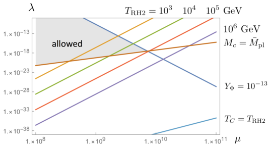
Figure 2: Allowed parameter region for $\lambda$ and $\mu$ in Scenario 1. Here we have taken $g_{*}=200$ and $g=1$.

A similar figure for Scenario 2 is shown in Fig. 3. The upper bound on the chemical potential is given as $\mu\lesssim 1.5\times 10^{9}$ GeV and the lower bound on $\lambda$ such that the thermal leptogenesis is operative is found to be $\lambda\gtrsim 7.5\times 10^{-21}$. The reheating temperature can be taken up to $8.6\times 10^{3}$ GeV, which is smaller than the one in Scenario 1.

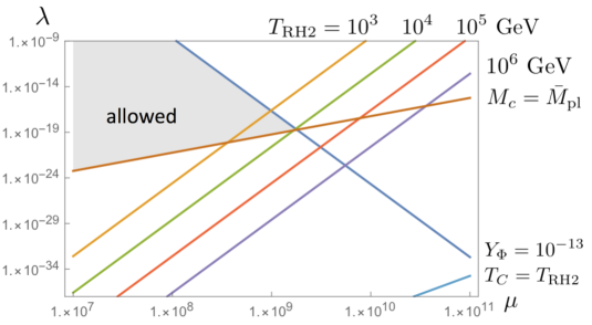
Figure 3: Same as Fig. 2 but for Scenario 2.

It should be emphasized that in the standard thermal inflation scenario, $T_{\rm RH2}$ cannot be large enough to implement the baryogenesis scenario except for the Affleck-Dine mechanism. The reheating temperature (18) is proportional to $\lambda^{1\over 4}$ and the flaton mass. Recalling that $m_{\phi}\simeq 1$ TeV and $\lambda$ should be small enough to satisfy (33), we see that $T_{\rm RH2}$ in the standard thermal inflation scenario is at most $\mathcal{O}(100)$ MeV. However, in our scenario the reheating temperature (56) is proportional to $\lambda^{-1/4}$ and $\mu^{2}$. Since $\mu$ is taken to be larger than $1$ TeV and in addition $\lambda$ can be taken to be small to satisfy (58) and (60) (but it is constrained by (62)), one can realize a reheating temperature high enough to implement the thermal leptogenesis.

4 Conclusion

In this paper, we have studied the models of the thermal inflation with the flaton chemical potential which is implemented naturally by the VEV of the zeroth component of the $U(1)_{c}$ (non-dynamical) gauge field. This leads to the negative mass squared of the flaton. On the other hand, in the standard thermal inflation, a negative mass squared of ${\cal O}(1)$ TeV, which is the soft SUSY breaking scale, can be realized by the renormalization group flow with a large coupling constant (most likely to be in the non-perturbative regime); otherwise, it is introduced by hand. We have evaluated the yield of the moduli in two scenarios: Moduli field start to oscillate before (Scenario 1) and after (Scenario 2) the reheating by the primordial inflation. In both scenarios, the yield depends on $\lambda$ being the coefficient of the sixth order term of the flaton potential and the chemical potential $\mu$. We have found the allowed parameter region in the $(\lambda,\mu)$-plane, in which after the thermal inflation the reheating temperature can be high enough for the thermal leptogenesis to be operative. This is in sharp contrast to the standard thermal inflation, in which the reheating temperature is at most ${\cal O}(100)$ MeV.

In this work we have introduced the flaton chemical potential as a free parameter. It is worth investigating a possible origin of the chemical potential in the framework of superstring theories. It is also interesting to consider a possibility to relate the global $U(1)_{c}$ to the baryon or the lepton numbers in the Standard Model.

Appendices

A Thermal 1-loop correction

In this appendix, we give a sketch of the derivations for (8) and (43). For the details, consult the references [35, 36].

At the 1-loop level, the correction of the effective potential from the thermal effect for a real scalar field is given by the determinant,

$$\log\left(\det\left(\partial^{2}+m^{2}\right)\right)^{1/2} = \frac{1}{2}{\rm tr}\;\log\left(\partial^{2}+m^{2}\right)$$ (A-1)

$$= \frac{1}{2\beta}\sum_{n=-\infty}^{+\infty}\int\frac{d^{3}k}{(2\pi)^{3}}\ \log\left((2\pi\beta^{-1}n)^{2}+\omega_{k}\right),$$

in the absence of the chemical potential. After formally differentiating (A-1) with respect to $\omega_{k}$, we can sum over the discrete momentum $2\pi\beta^{-1}n$,

$$\sum_{n=-\infty}^{+\infty}\frac{\partial}{\partial\omega_{k}}\log\left((2\pi\beta^{-1}n)^{2}+\omega_{k}^{2}\right) = \sum_{n=-\infty}^{+\infty}\frac{2\omega_{k}}{(2\pi\beta^{-1}n)^{2}+\omega_{k}^{2}}$$ (A-2)

$$= \sum_{n=-\infty}^{+\infty}\left(\frac{1}{\omega_{k}-i(2\pi\beta^{-1}n)}+\frac{1}{\omega_{k}+i(2\pi\beta^{-1}n)}\right)$$

$$= \beta\coth\left(\frac{\beta\omega_{k}}{2}\right).$$

Here we use the partial fraction expansion formula,

$$\pi\coth(\pi x)=\sum_{n=-\infty}^{+\infty}\frac{1}{x+in}.$$ (A-3)

Integrating (A-2) with $\omega_{k}$, we obtain

$$\log\left(\det\left(\partial^{2}+m^{2}\right)\right)^{1/2} \simeq \frac{1}{\beta}\int\frac{d^{3}k}{(2\pi)^{3}}\ \log\left|\sinh\left(\frac{\beta\omega_{k}}{2}\right)\right|$$ (A-4)

$$\simeq \int\frac{d^{3}k}{(2\pi)^{3}}\left(\frac{\omega_{k}}{2}+\frac{1}{\beta}\log\left|1-e^{-\beta\omega_{k}}\right|\right),$$

up to an irrelevant constant. In the case of a complex scalar, the correction is twice of that of a real scalar.

B Interaction terms of the flaton with the Standard Model sector

We consider the following higher dimensional term invariant under the $U(1)_{c}$ transformation for the flaton, $\phi\rightarrow e^{i\alpha}\phi$ associated with the chemical potential.

$${\cal L}_{\rm int}={1\over 4}\int d^{4}\theta\sum_{a=1}^{3}c_{a}{\Phi^{\dagger}\Phi\over\bar{M}_{\rm pl}^{2}}\left(W^{a\alpha}W^{a}_{\alpha}\delta^{2}(\bar{\theta})+h.c.\right)\,,$$ (B-1)

where $\Phi$ is a chiral superfield associated with the flaton and $W_{\alpha}^{a}$ is a superfield strength with the index $a=1,2,3$ corresponding to the Standard Model gauge groups $SU(3)\times SU(2)_{L}\times U(1)_{Y}$. In order to consider the interaction at the vacuum $\langle\Phi\rangle=M_{c}$, we substitute a shift

$$\Phi\rightarrow M_{c}+\Phi\,,$$ (B-2)

into (B-1) and pick up the following three-point vertex part:

$${\cal L}_{\rm int}\supset{M_{c}\over 4\bar{M}_{\rm pl}^{2}}\int d^{4}\theta\sum_{a=1}^{3}c_{a}(\Phi+\Phi^{\dagger})(W^{\alpha a}W^{a}_{\alpha}\delta^{2}(\bar{\theta})+h.c.)\,.$$ (B-3)

Since we are interested in the flaton decay, we focus on the scalar part of the flaton superfield, $\phi=\Phi|_{\theta=0}$ in (B-3):

$${\cal L}_{\rm int}\supset{M_{c}\over\bar{M}_{\rm pl}^{2}}\chi\sum_{a=1}^{3}c_{a}\left(-{1\over 4}F_{\mu\nu}^{a}F^{\mu\nu a}-i\lambda^{a}\sigma^{\mu}\partial_{\mu}\bar{\lambda}^{a}\right)\,,$$ (B-4)

where $\chi\equiv{\rm Re}(\phi)$, $F_{\mu\nu}^{a}$ and $\lambda^{a}$ are the field strength and the gaugino, respectively. This interaction leads to the decays $\chi\rightarrow A_{\mu}A_{\nu}$ and $\chi\rightarrow\lambda\bar{\lambda}$. The decay widths are obtained as $\Gamma(\chi\rightarrow A_{\mu}A_{\nu})\propto(M_{c}/\bar{M}_{\rm pl}^{2})^{2}\mu^{3}$ and $\Gamma(\chi\rightarrow\lambda\bar{\lambda})\propto(M_{c}/\bar{M}_{\rm pl}^{2})^{2}m_{\lambda}^{2}\mu$, where $m_{\lambda}\simeq 1$ TeV is the gaugino mass. Since we take $\mu\gg 1$ TeV in our scenario (see Figs. 2 and 3), the flaton mainly decays to the Standard Model gauge bosons.

Acknowledgments

This work is supported in part by the Japan Society for the Promotion for Science Grant-in-Aid for Scientific Research (KAKENHI) Grant Numbers 25400280 (M.A.), the United States Department of Energy (DE-SC001368)(N.O.) and Kitasato University Research Grant for Young Researchers (S.S.).

References

- [1] K. Sato, “First Order Phase Transition of a Vacuum and Expansion of the Universe,” Mon. Not. Roy. Astron. Soc. 195 (1981) 467.
- [2] A. H. Guth, “The Inflationary Universe: A Possible Solution to the Horizon and Flatness Problems,” Phys. Rev. D 23 (1981) 347.
- [3] A. A. Starobinsky, “A New Type of Isotropic Cosmological Models Without Singularity,” Phys. Lett. 91B (1980) 99.
- [4] A. D. Linde, “A New Inflationary Universe Scenario: A Possible Solution of the Horizon, Flatness, Homogeneity, Isotropy and Primordial Monopole Problems,” Phys. Lett. 108B (1982) 389.
- [5] A. Albrecht and P. J. Steinhardt, “Cosmology for Grand Unified Theories with Radiatively Induced Symmetry Breaking,” Phys. Rev. Lett. 48 (1982) 1220.
- [6] H. Pagels and J. R. Primack, “Supersymmetry, Cosmology and New TeV Physics,” Phys. Rev. Lett. 48 (1982) 223.
- [7] S. Weinberg, “Cosmological Constraints on the Scale of Supersymmetry Breaking,” Phys. Rev. Lett. 48 (1982) 1303.
- [8] L. M. Krauss, “New Constraints on Ino Masses from Cosmology. 1. Supersymmetric Inos,” Nucl. Phys. B 227 (1983) 556.
- [9] M. Kawasaki, K. Kohri and T. Moroi, “Hadronic decay of late - decaying particles and Big-Bang Nucleosynthesis,” Phys. Lett. B 625, 7 (2005) [astro-ph/0402490].
- [10] M. Kawasaki, K. Kohri and T. Moroi, “Big-Bang nucleosynthesis and hadronic decay of long-lived massive particles,” Phys. Rev. D 71 (2005) 083502 [astro-ph/0408426].
- [11] G. D. Coughlan, W. Fischler, E. W. Kolb, S. Raby and G. G. Ross, “Cosmological Problems for the Polonyi Potential,” Phys. Lett. B 131 (1983) 59.
- [12] T. Banks, D. B. Kaplan and A. E. Nelson, “Cosmological implications of dynamical supersymmetry breaking,” Phys. Rev. D 49 (1994) 779 [hep-ph/9308292].
- [13] B. de Carlos, J. A. Casas, F. Quevedo and E. Roulet, “Model independent properties and cosmological implications of the dilaton and moduli sectors of 4-d strings,” Phys. Lett. B 318 (1993) 447 [hep-ph/9308325].
- [14] D. H. Lyth and E. D. Stewart, “Cosmology with a TeV mass GUT Higgs,” Phys. Rev. Lett. 75 (1995) 201 [hep-ph/9502417].
- [15] D. H. Lyth and E. D. Stewart, “Thermal inflation and the moduli problem,” Phys. Rev. D 53 (1996) 1784 [hep-ph/9510204].
- [16] E. D. Stewart, M. Kawasaki and T. Yanagida, “Affleck-Dine baryogenesis after thermal inflation,” Phys. Rev. D 54 (1996) 6032 [hep-ph/9603324].
- [17] T. Barreiro, E. J. Copeland, D. H. Lyth and T. Prokopec, “Some aspects of thermal inflation: The Finite temperature potential and topological defects,” Phys. Rev. D 54 (1996) 1379 [hep-ph/9602263].
- [18] T. Asaka, J. Hashiba, M. Kawasaki and T. Yanagida, “Cosmological moduli problem in gauge mediated supersymmetry breaking theories,” Phys. Rev. D 58 (1998) 083509 [hep-ph/9711501].
- [19] T. Asaka and M. Kawasaki, “Cosmological moduli problem and thermal inflation models,” Phys. Rev. D 60 (1999) 123509 [hep-ph/9905467].
- [20] T. Hiramatsu, Y. Miyamoto and J. Yokoyama, “Effects of thermal fluctuations on thermal inflation,” JCAP 1503 (2015) 03, 024 [arXiv:1412.7814 [hep-ph]].
- [21] T. Hayakawa, M. Kawasaki and M. Yamada, “Can thermal inflation be consistent with baryogenesis in gauge-mediated SUSY breaking models?,” Phys. Rev. D 93 (2016) no.6, 063529 [arXiv:1508.03409 [hep-ph]].
- [22] H. Murayama, H. Suzuki and T. Yanagida, “Radiative breaking of Peccei-Quinn symmetry at the intermediate mass scale,” Phys. Lett. B 291 (1992) 418.
- [23] J. R. Ellis, G. B. Gelmini, J. L. Lopez, D. V. Nanopoulos and S. Sarkar, “Astrophysical constraints on massive unstable neutral relic particles,” Nucl. Phys. B 373 (1992) 399.
- [24] K. Yamamoto, “Saving the Axions in Superstring Models,” Phys. Lett. 161B (1985) 289.
- [25] I. Affleck and M. Dine, “A New Mechanism for Baryogenesis,” Nucl. Phys. B 249 (1985) 361.
- [26] M. Dine, L. Randall and S. D. Thomas, “Baryogenesis from flat directions of the supersymmetric standard model,” Nucl. Phys. B 458 (1996) 291 [hep-ph/9507453].
- [27] M. Fukugita and T. Yanagida, “Baryogenesis Without Grand Unification,” Phys. Lett. B 174 (1986) 45.
- [28] W. Buchmuller, P. Di Bari and M. Plumacher, “Leptogenesis for pedestrians,” Annals Phys. 315 (2005) 305 [hep-ph/0401240].
- [29] M. Dine, V. Kaplunovsky, M. L. Mangano, C. Nappi and N. Seiberg, “Superstring Model Building,” Nucl. Phys. B 259 (1985) 549.
- [30] A. Actor, “Chemical Potentials In Gauge Theories,” Phys. Lett. B 157 (1985) 53; “Zeta Function Regularization Of High Temperature Expansions In Field Theory,” Nucl. Phys. B 265 (1986) 689.
- [31] A. G. Cohen, D. B. Kaplan and A. E. Nelson, “Progress in electroweak baryogenesis,” Ann. Rev. Nucl. Part. Sci. 43 (1993) 27 [hep-ph/9302210].
- [32] P. S. Bhupal Dev, P. Millington, A. Pilaftsis and D. Teresi, “Flavour Covariant Transport Equations: an Application to Resonant Leptogenesis,” Nucl. Phys. B 886, 569 (2014) [arXiv:1404.1003 [hep-ph]].
- [33] R. Harnik, D. T. Larson and H. Murayama, “Supersymmetric color superconductivity,” JHEP 0403 (2004) 049 [hep-ph/0309224].
- [34] H. Itoh, N. Okada and T. Yamashita, “Low scale gravity mediation with warped extra dimension and collider phenomenology on the hidden sector,” Phys. Rev. D 74 (2006) 055005 [hep-ph/0606156].
- [35] C. W. Bernard, “Feynman Rules for Gauge Theories at Finite Temperature,” Phys. Rev. D 9, 3312 (1974).
- [36] L. Dolan and R. Jackiw, “Symmetry Behavior at Finite Temperature,” Phys. Rev. D 9, 3320 (1974).