Chemical abundance analysis of 13 southern symbiotic giants from high-resolution spectra at $\sim$1.56 $\mu$m

Abstract

Symbiotic stars (SySt) are binaries composed of a star in the later stages of evolution and a stellar remnant. The enhanced mass-loss from the giant drives interacting mass exchange and makes these systems laboratories for understanding binary evolution. Studies of the chemical compositions are particularly useful since this parameter has strong impact on the evolutionary path. The previous paper in this series presented photospheric abundances for 24 giants in S-type SySt enabling a first statistical analysis. Here, we present results for an additional sample of 13 giants. The aims are to improve statistics of chemical composition involved in the evolution of SySt, to study evolutionary status, mass transfer and to interpret this in terms of Galactic populations. High resolution, near-IR spectra are used, employing the spectrum synthesis method in a classical approach, to obtain abundances of CNO and elements around the iron peak (Fe, Ti, Ni). Low resolution spectra in the region around the Ca ii triplet were used for spectral classification. The metallicities obtained cover a wide range with a maximum around $\sim-0.2$ dex. The enrichment in the ¹⁴N isotope indicates that these giants have experienced the first dredge-up. Relative O and Fe abundances indicate that most SySt belong to the Galactic disc; however, in a few cases, the extended thick-disc/halo is suggested. Difficult to explain, relatively high Ti abundances can indicate that adopted microturbulent velocities were too small by $\sim$0.2–0.3 km s^-1 . The revised spectral types for V2905 Sgr, and WRAY 17-89 are M3 and M6.5, respectively.

1 Introduction

Symbiotic stars (SySt) are among the longest orbital period interacting binaries. They are composed of a cool giant as the primary component and a secondary that is a remnant of the latest stages of stellar evolution – typically a white dwarf (WD) but a neutron star is also suggested in a few cases. The giant member is losing matter at a high rate, up to about 10^-7M☉ yr^-1, a rate systematically higher than for single field giants (Mikołajewska, Ivison & Omont, 2003, and references therein). Interactions of the mass flow with hard radiation from the hot, luminous remnant results in a complex environment around each component of the system with many systems being embedded in an ionized nebula. The bulk of the giant’s mass outflow ultimately can be lost from the system. However, a substantial part can be accreted on to the compact object directly from the giant wind and/or via Roche lobe overflow (Podsiadlowski & Mohamed, 2007). When the system formed the current remnant was the more massive component. As this star evolved, mass was transferred on to the star that is now the giant and traces of this mass transfer may be detectable in the observed chemical composition of the current red giant. There is clear evidence for this history of binary evolution in the S-type symbiotic systems. Most systems have orbital periods below $\sim$1000 d and circularized orbits that indicate that mass transfer and strong interactions took place before the present WD was formed (Mikołajewska, 2012).

Chemical composition is secondary only to initial stellar mass in determining stellar evolution. In binary systems where abundances are modified due to mass transfer, the information about single and binary evolution becomes entangled. However, abundances of some specific kinds of chemical elements, eg. s-process elements produced during the AGB phase and/or CNO abundances, combined with theoretical limitations and known basic parameters of the stars in the system enable us to deduce the interactions and history of the mass exchange between components. This motivated us to determine chemical abundances in S-type symbiotic giants with the goal of understanding their evolution. Including new results presented here abundances are known for more than 40 red giants in SySt. Statistical analysis (Gałan et al., 2016, Paper III) addresses metallicity (from its proxy the iron abundance), evolutionary status (by analysis of carbon and nitrogen abundances and ¹²C/¹³C ratio), and Galactic population membership (by analysis of the alpha-element abundances, titanium and oxygen, relative to iron).

In this paper, we present chemical compositions (abundances of CNO and elements around the iron peak: Fe, Ti, Ni) for a sample of 13 red giants in S-type symbiotic systems located in the Southern hemisphere. The abundances are measured using high-resolution near-IR spectra. This is another step in building a statistical base for future analysis of SySt samples representing all stellar populations and various locations in the Milky Way and the Magellanic Clouds. The structure of the paper is as follows. Section 2 lists and describes our spectroscopic observations. Section 3 specifies the methods used and presents the results. The results are discussed briefly with comparison to our previous sample in Section 4.

Table 1: Journal of spectroscopic observations.

	Id.a	Date	HJD (mid)	Phaseb	Range
		dd.m.yy	$-2450000$		[$\mu$m]
WRAY 15-1470	63	24.5.10	5340.5687	0.23	$\sim$1.56
Hen3 1341	74	24.5.10	5340.6483	0.38	$\sim$1.56
WRAY 17-89	85	24.5.10	5340.6666	–	$\sim$1.56
		23.3.16	7470.5698	–	$\sim$0.86
V2416 Sgr	113	03.6.10	5350.6669	–	$\sim$1.56
V615 Sgr	123	24.5.10	5340.9227	0.83	$\sim$1.56
AS 281	127	27.6.10	5374.7624	0.92	$\sim$1.56
V2756 Sgr	133	02.6.10	5349.8471	0.20	$\sim$1.56
V2905 Sgr	139	04.6.10	5351.9279	0.33	$\sim$1.56
		21.3.16	7468.6330	0.49	$\sim$0.86
AR Pav	142	06.6.09	4988.9345	0.33	$\sim$1.56
		26.5.10	5342.7892	0.92	$\sim$1.56
V3804 Sgr	144	03.8.09	5046.7705	0.47	$\sim$1.56
V4018 Sgr	147	09.6.10	5356.6536	0.29	$\sim$1.56
V919 Sgr	159	03.8.09	5046.7861	–	$\sim$1.56
CD$-$43°14304	182	06.6.09	4988.8972	0.51	$\sim$1.56
		26.5.10	5342.7708	0.75	$\sim$1.56
HR 6020	–	21.3.16	7468.5838	–	$\sim$0.86
HD 70421	–	22.3.16	7470.2712	–	$\sim$0.86
HR 1247	–	22.3.16	7470.2880	–	$\sim$0.86
HR 1264	–	22.3.16	7470.2954	–	$\sim$0.86
HR 3718	–	22.3.16	7470.3270	–	$\sim$0.86
HR 4902	–	22.3.16	7470.4247	–	$\sim$0.86
SW Vir	–	22.3.16	7470.4361	–	$\sim$0.86

• Identification number according to Belczyński et al. (2000).

• Orbital phases that correspond to photometric minima (giant in the front) are taken in majority from Gromadzki et al. (2013): WRAY 15-1470 2451845+561$\times$E; Hen3 1341 2451970+626$\times$E; V615 Sgr 2452168+657$\times$E; AS 281 2449021+533$\times$E; V2756 Sgr 2451894+480$\times$E; V2905 Sgr 2451630+508$\times$E; V3804 Sgr 2451439+426$\times$E; V4018 Sgr 2452129+513$\times$E; from Schild et al. (2001): 2448139+604.5$\times$E for AR Pav; and for CD$-$43°14304 from ephemeris 2447015+1448$\times$E recalculated according to circular orbit case (Schmid et al., 1998).

2 Observations and data reduction

Near-IR spectra of 13 symbiotic SySt were observed in 2009 June, 2009 August, 2010 May and 2010 June using the Phoenix cryogenic echelle spectrograph on the 8-m Gemini-S telescope. The spectra were obtained through a poor weather observing programme. All are characterized by high resolving power ($R\sim 50000$) and most by high-S/N ratio ($\sim$ 100). The Gaussian instrumental profile is $\sim$6 km s^-1 full width at half-maximum (FWHM), corresponding to $\sim$0.31Å at the observed wavelength. The spectra cover narrow spectral intervals ($\sim$60Å) located in wavelength range between 1.560–1.568 µm. This region, free of telluric features, is dominated by first overtone OH lines and numerous neutral atomic lines Fe i, Ti i, Ni i plus a number of generally weak CN red system, $\Delta v=-1$ lines and CO second-overtone vibration–rotation lines. The selected absorption lines are useful to measure abundances of carbon, nitrogen, oxygen and elements around the iron peak: Ti, Fe and Ni.

The spectra were extracted from the raw data and wavelength calibrated using standard reduction techniques (Joyce, 1992). The wavelength scales were heliocentric corrected. The IRAF cross-correlation program FXCOR was employed (Fitzpatrick, 1993) to shift the observed spectra, removing the stellar radial velocity, to the wavelength of the spectral lines in synthetic spectra. Representative spectra with synthetic fits are shown in Figs 1 and 2. The spectra selected, CD$-$43°14304 and AS 281, are the most blueshifted and redshifted, respectively, to show the whole explored wavelength range.

Lower resolution, very near-infrared spectra were also observed around the Ca ii triplet ($\lambda\sim$ 7200–9600 Å, $R\sim 2200$, S/N $\sim 50$) for two symbiotic systems (V2905 Sgr and WRAY 17-89) and several M-type giant standard stars with the Cassegrain spectrograph (grating nr 11) operated on 1.9 m ’Radcliffe’ telescope in Sutherland (South African Astronomical Observatory). The observation took place in 2016 March as part of our project (JM, CG) to look for the evidences of enhancement of giants with s-process elements from previous accretion. These spectra were used here to improve in classification of the spectral type. The journal of our spectroscopic observations is shown in Table 1.

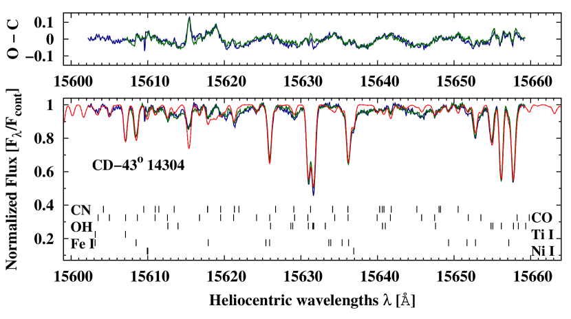
Figure 1: Spectra of CD$-$43°14304 observed 2009 June (blue line), 2010 May (green line) and synthetic spectra (red continuous and dashed lines) calculated using the final abundances (Table 4).

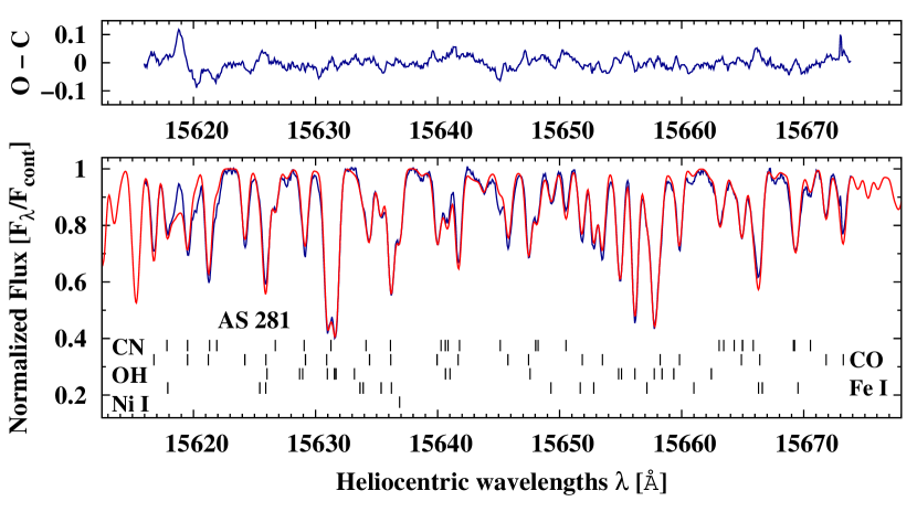
Figure 2: The spectrum of AS 281 observed 2010 June (blue line) and a fitted synthetic spectrum (red line).

Table 2: Stellar parameters: effective temperature $T_{\rm{eff}}$ and surface gravity $\log{g}$.

	Spec.	$T_{\rm{eff}}^{[1]}$	$T_{\rm{eff}}^{[2]}$	$J-K^{[3,4]}$	$E$($B-V$)[5]	($J-K$)0	$T_{\rm{eff}}^{[6]}$	$\log{g}$[6]	$\log{g}$[7]	$T_{\rm{eff}}^{a}$	$\log{g}^{a}$
	Type	[K]	[K]	mag	mag	mag	[K]			[K]
WRAY 15-1470	M3[8]	3560$\pm$75	3586	1.38$\pm$0.07	$<$0.49$\pm$0.02	$>$1.15$\pm$0.07	$<$3570$\pm$140	$<$+0.5$\pm$0.3	0.5–0.8	3600	0.5
Hen 3-1341	M4[8]	3460$\pm$75	3476	1.32$\pm$0.07	$<$0.31$\pm$0.01	$>$1.17$\pm$0.09	$<$3520$\pm$180	$<$+0.4$\pm$0.3	0.4–0.7	3500	0.5
WRAY 17-89	M6.5[11]	3170$\pm$80	3203	2.06$\pm$0.07	$<$1.49$\pm$0.05	$>$1.33$\pm$0.13	$<$3200$\pm$260	$<$-0.1$\pm$0.5	0.0–0.3	3200	0.0
V2416 Sgr	M6[8]	3240$\pm$75	3258	1.99$\pm$0.08	–	–	–	–	0.1–0.4	3300	0.0
V615 Sgr	M5.5[8]	3300$\pm$75	3312	1.32$\pm$0.06	$<$0.15$\pm$0.01	$>$1.25$\pm$0.07	$<$3360$\pm$150	$<$+0.1$\pm$0.3	0.2–0.5	3300	0.0
AS 281	M6b	3240$\pm$75	3258	1.49$\pm$0.06	$<$0.48$\pm$0.03	$>$1.26$\pm$0.10	$<$3340$\pm$200	$<$+0.1$\pm$0.4	0.1–0.4	3300	0.0
V2756 Sgr	M4b	3460$\pm$75	3476	1.34$\pm$0.06	$<$0.27$\pm$0.01	$>$1.21$\pm$0.08	$<$3440$\pm$160	$<$+0.3$\pm$0.3	0.4–0.7	3500	0.5
V2905 Sgr	M3[11]	3560$\pm$75	3586	1.26$\pm$0.07	$<$0.28$\pm$0.01	$>$1.13$\pm$0.08	$<$3610$\pm$170	$<$+0.6$\pm$0.3	0.5–0.8	3600	0.5
AR Pav	M5[8]	3355$\pm$75	3367	1.17$\pm$0.07	$<$0.08$\pm$0.01	$>$1.13$\pm$0.08	$<$3610$\pm$170	$<$+0.6$\pm$0.3	0.3–0.6	3400	0.0
V3804 Sgr	M5[9]	3355$\pm$75	3367	1.46$\pm$0.06	$<$0.21$\pm$0.01	$>$1.35$\pm$0.07	$<$3150$\pm$130	$<$-0.2$\pm$0.2	0.3–0.6	3300	0.0
V4018 Sgr	M4[10]	3460$\pm$75	3476	1.24$\pm$0.06	$<$0.34$\pm$0.01	$>$1.09$\pm$0.08	$<$3690$\pm$160	$<$+0.7$\pm$0.3	0.4–0.7	3500	0.5
V919 Sgr	M4.5[8]	3410$\pm$75	3421	1.38$\pm$0.07	$<$0.21$\pm$0.01	$>$1.27$\pm$0.07	$<$3310$\pm$150	$<$+0.1$\pm$0.3	0.3–0.6	3400	0.5
CD$-$43°14304	K7[8]	$\sim$3910	$\sim$3980	1.08$\pm$0.09	$<$0.03$\pm$0.01	$>$1.07$\pm$0.09	$<$3740$\pm$190	$<$+0.8$\pm$0.4	–	3900	1.0

• total Galactic extinction according to ^[5]Schlafly & Finkbeiner (2011) and Schlegel, Finkbeiner & Davis (1998), infrared colours from 2MASS ^[3](Phillips, 2007) transformed to ^[4]Bessell & Brett (1988) photometric system. Spectral types are from: ^[8]Mürset & Schmid (1999), ^[9] Medina Tanco & Steiner (1995), ^[10] Allen (1980), ^[11] this work

• ^[1]Richichi et al. (1999), ^[2]Van Belle et al. (1999), ^[6]Kucinskas et al. (2005), ^[7]Dumm & Schild (1998).

• adopted.

• spectral types changed to later by one spectral subclass relative to Medina Tanco & Steiner (1995) spectral classification.

3 Analysis and results

To measure chemical abundances we used spectral synthesis techniques employing local thermodynamic equilibrium (LTE) analysis. The model atmospheres were from a 1D, hydrostatic MARCS model atmospheres (Gustafsson et al., 2008). This analysis was also employed in previous papers (Mikołajewska et al. 2014, (Paper I), Gałan, Mikołajewska & Hinkle 2015, (Paper II), Gałan et al. 2016, (Paper III)). Justifications for the adopted methodology can be found there. The excitation potentials and $gf$-values for transitions were taken in the case of atomic lines from the list by Mélendez & Barbuy (1999) and for the molecular data we used line lists by Goorvitch (1994) for CO, by Kurucz (1999) for OH and by Sneden et al. (2014) for CN. The WIDMO code developed by M. R. Schmidt (Schmidt et al., 2006) was used to calculate synthetic spectra.

Table 3: Spectral classification of V2905 Srg, and WRAY 17-89 based on the strength of five TiO band heads.

	TiO band head ($\lambda$ [Å]).
	7589	8194	8432	8859	9209	Mean
V2905 Sgr	M3	$\leq$M2	M4–3.5	$<$M3	$\leq$M4	M3
WRAY 17-89	M5	M6	M5.5a	M6	M7	M6

• can be significantly shallowed by the emission in Ca ii triplet.

In summary the abundances calculations were performed as follows. The starting values of abundances were obtained by fitting by eye, through several iterations, alternately from molecular and atomic lines. Next, the simplex algorithm (Brandt, 1998) was used for $\chi^{2}$ minimization with seven free parameters: C, N, O, Fe, Ti, Ni abundances and the rotational velocity. The rotational velocity must in this case be treated as a free parameter because there was no way to measure reliably its value from severely blended spectra. A number of atmosphere models have been tested with the above procedure for each target, when needed, to choose the one with the best-matching metallicity. The stellar parameters, effective temperature ($T_{\rm{eff}}$) and surface gravity ($\log{g}$), could not be measured directly from our spectra because of lack the lines from ionized elements and unblended lines with different intensities for the same elements. The atmospheric parameters needed for selecting the most suitable atmosphere model were instead derived from the spectral types (Table 2). In most cases, the spectral types were derived from TiO bands in the near-IR with high accuracy of approximately one spectral subclass (Mürset & Schmid, 1999).

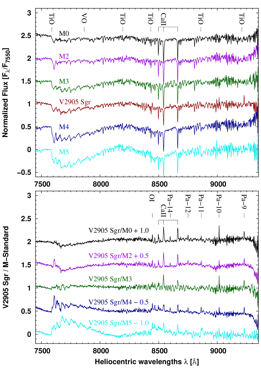
Figure 3: The spectrum of V2905 Sgr (red) is compared with the spectra of spectroscopic standards (top) that are giants of types from M5 to M0. At the bottom ratios of the V2905 Sgr spectrum with the spectra of standards. The spectra are shifted by 0.5 for clarity. The flattest spectrum around the value one results from division by the M3 standard spectrum (green). The contribution from nebular continuum is seen in emission from Ca ii triplet, OI ($\lambda$ 8442.36 Å) and numerous lines of the Paschen series.

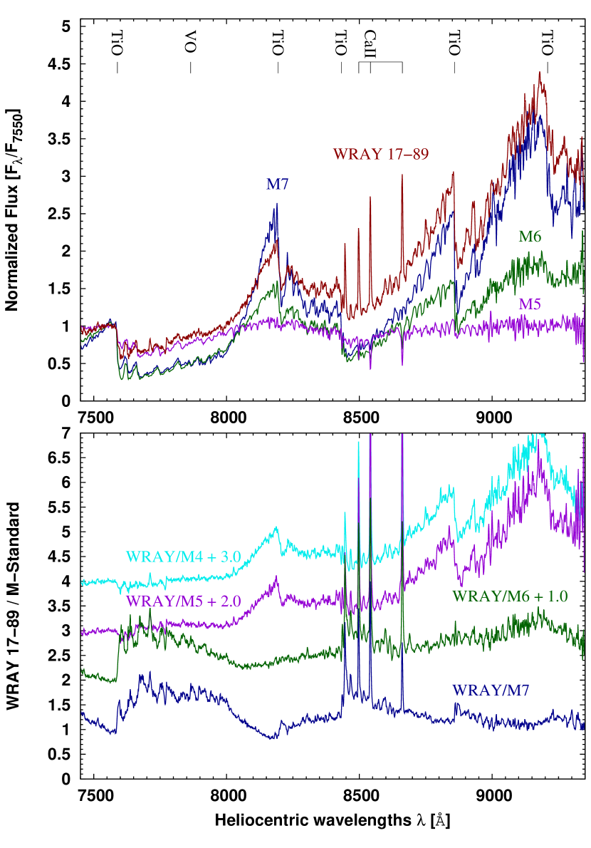
Figure 4: The spectrum of WRAY 17-89 (red) is compared with the spectra of spectroscopic standards (top) that are giants of spectral types M7, M6 and M5. At the bottom the ratios of the WRAY 17-89 spectrum with the spectra of standards are presented (the spectra are shifted by 1.0 for clarity).

V2905 Sgr and WRAY 17-89 were classified by Mikołajewska et al. (1997) as giants of spectral types M0 and M3, respectively. We found that this classification based on optical spectra resulted in a too early spectral type. We used near-infrared spectra around the Ca ii triplet to improve the spectral type classification. This domain is particularly useful in studying properties of the late-type stars in SySt because they are intrinsically bright in this range and contamination by the nebula and hot component is negligible. To determine the spectral types, we used a method similar to Mürset & Schmid (1999) with two approaches. (i) In one approach, the strength of TiO features in the spectrum of SySt were compared by eye with those in the spectra of M-type giant standard stars with well-known spectral types: HR 3718 (M0, Mürset & Schmid (1999)), HR 1247, HR 4902, HR 1264, HR 6020, SW Vir (M2, M3, M4, M5 and M7, respectively Feast et al. (1990)) and HD 70421 (M6, Schulte-Ladbeck (1988)). Several TiO bands with the heads at $\sim$ 7589, 8194, 8432, 8859 and 9209 Å are especially useful. (ii) In the second approach, the SySt spectrum divided by the standard spectrum is assessed for the smoothest ratio. Interestingly, the Ca ii triplet itself is a diagnostic of temperature and luminosity class as well as metallicity for ’normal’, singular red giants of early spectral types. However, it does not work for giants interacting in symbiotic systems. In the symbiotics the Ca ii lines are frequently modified by strong contribution from nebula, as clearly seen in the case of V2905 Sgr (Fig.3, bottom).

For V2905 Sco, the spectral types from the depths of TiO band heads are in the range M2–M4 with the average around M3 (Table 3). The strong TiO band with the head at $\lambda\sim 7589\AA$ clearly indicates an M3 type (Fig. 3, top). The mean spectra resulting from division of V2905 Sgr spectrum by the spectral standards achieve the smallest deviations from flatness for the spectral type M3 (Fig. 3, bottom). A visual comparison of the spectrum of V2905 Sgr to the standards shows that the spectrum is a best match to M3 at shorter wavelengths and in the long wavelength range is earlier than M4. Therefore, we adopt M3 as the most suitable classification for this giant.

For WRAY 17-89 the depths of TiO bands indicate an M6 spectral type (Table 3, and Fig. 4, top). The result of division of the WRAY 17-89 spectrum by the spectral standards gives the smallest deviation from flatness for M7 (Fig. 4, bottom). From a visual comparison, the spectrum at longer wavelengths resemble an M7 giant while at the short wavelength M6-5 is a better match. We adopted M6.5-type for this star.

Adopting M3 and M6.5 spectral types for the giants in V2905 Sgr, and WRAY 17-89, respectively, gives excellent agreement between the effective temperatures obtained from the spectral types and those estimated from infrared colours (Table 2).

In the case of two other objects, AS 281 and V2756 Sgr, we found that the spectral types by Medina Tanco & Steiner (1995), M5 and M3 respectively, seem too early. We do not have 7200–9600 Å spectra for these objects. However, we reanalyzed the published spectra looking at the strength of TiO bands heads and the VO band head at 7865 Å. We have reclassified the spectral types by one subclass to M6 and M4, respectively. The method of classification by Medina Tanco & Steiner (1995) typically leads to earlier spectral types than the classification by Mürset & Schmid (1999) for the same objects. For this reason, we previously (Gałan et al., 2016) reclassified the spectral type of SS73 96.

To derive $T_{\rm{eff}}$, the calibrations of Richichi et al. (1999) and Van Belle et al. (1999) were used. The surface gravity was estimated using two methods. In the first technique, upper limits to $\log{g}$ were found from the $T_{\rm{eff}}$–$\log{g}$–colour relation for late-type giants (Kucinskas et al., 2005). Infrared intrinsic colours were derived from known $J$ and $K$ magnitudes (Phillips, 2007) corrected for extinction by adopting colour excesses from the Schlafly & Finkbeiner (2011) maps of the Galactic extinction. The temperatures derived from spectral types are in general within the limits on the temperatures derived from dereddened ($J-K$)₀ colours. The second method derives the radius of the giant star from the radius–spectral type relation Dumm & Schild (1998, Table 2) by assuming that the typical mass of giant in the S-type symbiotic systems is $\sim$1–2 M☉  (Mikołajewska, 2003). Values of $T_{\rm{eff}}$ and $\log{g}$ for the model atmospheres used to synthesize the spectra are shown in the rightmost columns of Table 2.

AR Pav is an eclipsing binary so an additional constraint can be placed on the $\log{g}$ value. With the orbital inclination known Quiroga et al. (2002) were able to solve for the mass and radius from the solution to the red giant’s orbital parameters. The giant’s mass is $M_{\rm{rg}}=2.5\pm 0.6$M☉. The giant’s radius is 137$\pm 20$R☉  if the orbit is seen edge on and ranges up to $\sim 210$R☉  for the maximum allowed inclination, $i\approx 70$°. The giant nearly fills its Roche lobe so is assumed to be tidally distorted. The resulting range for the surface gravity is $\log{g}\approx$0.1–0.8. Observations of infrared light variation resulting from ellipsoidal changes suggest that the giant is tidally distorted with $R_{\rm{rg}}=\sim 190$R☉  Rutkowski et al. (2007). With this value $\log{g}=0$, close to the lower limit. This is in good agreement with values for other symbiotic giants listed in Table 2.

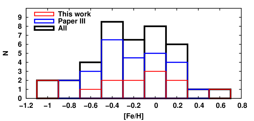
Figure 5: The distribution for the number ’N’ of objects, counted at 0.2 dex intervals, as a function of metallicity ([Fe/H]) for all symbiotic giants studied by us so far including two samples (black): the current sample (red) based on $H$-band spectra only, and previous sample (blue) obtained from analysis of both $H$- and $K$-band regions (Paper III).

The parameters describing the atmospheric motion, the micro ($\xi_{\rm t}$) and macro ($\zeta_{\rm t}$) turbulence velocities, were set to typical values for cool Galactic red giants. The most commonly used values are $\xi_{\rm{t}}=2$ km s^-1 and $\zeta_{\rm{t}}$ = 3 km s^-1 (see Paper III).

Table 4: Final abundances derived on the scale of $\log{\epsilon}(X)=\log{(N(X)N(H)^{-1})}+12.0$, abundances relative to solar abundances together with the formal fitting errors ^a, and rotational velocities.

	C	N	O	Ti	Fe	Ni	$V_{\rm{rot}}\sin{i}$	$V_{\rm{rot}}\sin{i}$
	$\log{\epsilon(X)}$						$[\rm{km}\,\rm{s}^{-1}]$	$[\rm{km}\,\rm{s}^{-1}]$
	[$X$]b						(FIT)	(CCF)
WRAY 15-1470	$8.03\pm 0.02$	$7.77\pm 0.04$	$8.77\pm 0.01$	–	$7.21\pm 0.04$	$5.83\pm 0.07$	5.4$\pm$0.4	4.5$\pm$0.8
	$-0.40\pm 0.07$	$-0.06\pm 0.09$	$+0.08\pm 0.06$	–	$-0.26\pm 0.08$	$-0.37\pm 0.11$
Hen 3-1341	$7.90\pm 0.01$	$7.75\pm 0.02$	$8.53\pm 0.01$	$4.80\pm 0.06$	$6.93\pm 0.02$	$5.75\pm 0.04$	6.6$\pm$0.1	5.3$\pm$0.4
	$-0.53\pm 0.06$	$-0.08\pm 0.07$	$-0.16\pm 0.06$	$-0.13\pm 0.10$	$-0.54\pm 0.06$	$-0.45\pm 0.08$
WRAY 17-89	$8.86\pm 0.03$	$9.05\pm 0.11$	$9.78\pm 0.04$	$5.56\pm 0.18$	$8.14\pm 0.05$	$6.15\pm 0.12$	9.5$\pm$0.2	6.3$\pm$0.4
	$+0.43\pm 0.08$	$+1.22\pm 0.16$	$+1.09\pm 0.09$	$+0.63\pm 0.22$	$+0.67\pm 0.09$	$-0.05\pm 0.16$
V2416 Sgr	$8.43\pm 0.03$	$8.57\pm 0.10$	$9.05\pm 0.02$	$5.54\pm 0.09$	$7.67\pm 0.06$	$6.29\pm 0.09$	7.7$\pm$0.3	6.1$\pm$0.6
	$0.00\pm 0.08$	$+0.74\pm 0.15$	$+0.36\pm 0.07$	$+0.61\pm 0.13$	$+0.20\pm 0.10$	$+0.09\pm 0.13$
V615 Sgr	$7.91\pm 0.04$	$8.30\pm 0.12$	$8.66\pm 0.03$	$5.06\pm 0.12$	$7.40\pm 0.03$	$6.16\pm 0.11$	7.0$\pm$0.5	6.0$\pm$0.5
	$-0.52\pm 0.09$	$+0.47\pm 0.17$	$-0.03\pm 0.08$	$+0.13\pm 0.16$	$-0.07\pm 0.07$	$-0.04\pm 0.15$
AS 281	$7.94\pm 0.04$	$7.53\pm 0.10$	$8.27\pm 0.01$	–	$7.11\pm 0.04$	$6.23\pm 0.12$	6.1$\pm$0.3	5.7$\pm$0.8
	$-0.49\pm 0.09$	$-0.30\pm 0.15$	$-0.42\pm 0.06$	–	$-0.36\pm 0.08$	$+0.03\pm 0.16$
V2756 Sgr	$8.23\pm 0.02$	$7.96\pm 0.07$	$8.81\pm 0.04$	$4.85\pm 0.10$	$7.39\pm 0.03$	$6.03\pm 0.09$	8.0$\pm$0.5	6.9$\pm$0.6
	$-0.20\pm 0.07$	$+0.13\pm 0.12$	$+0.12\pm 0.09$	$-0.08\pm 0.14$	$-0.08\pm 0.07$	$-0.17\pm 0.13$
V2905 Sgr	$7.33\pm 0.04$	$7.41\pm 0.06$	$7.89\pm 0.04$	–	$6.44\pm 0.03$	$5.50\pm 0.09$	9.7$\pm$0.6	–
	$-1.10\pm 0.09$	$-0.42\pm 0.11$	$-0.80\pm 0.09$	–	$-1.03\pm 0.07$	$-0.70\pm 0.13$
AR Pav	$7.86\pm 0.02$	$7.91\pm 0.05$	$8.51\pm 0.02$	$4.51\pm 0.18$	$7.22\pm 0.04$	$5.82\pm 0.09$	11.1$\pm$0.7	10.5$\pm$0.6
	$-0.58\pm 0.07$	$+0.08\pm 0.10$	$-0.19\pm 0.07$	$-0.43\pm 0.22$	$-0.26\pm 0.08$	$-0.38\pm 0.13$	8.7$\pm$0.4	8.1$\pm$1.4
V3804 Sgr	$8.16\pm 0.01$	$7.89\pm 0.03$	$8.60\pm 0.02$	$4.81\pm 0.06$	$7.52\pm 0.01$	$5.84\pm 0.04$	10.0$\pm$0.2	8.2$\pm$0.3
	$-0.27\pm 0.06$	$+0.06\pm 0.08$	$-0.09\pm 0.07$	$-0.12\pm 0.10$	$+0.05\pm 0.05$	$-0.36\pm 0.08$
V4018 Sgr	$8.48\pm 0.02$	$8.26\pm 0.03$	$9.00\pm 0.02$	$5.16\pm 0.08$	$7.67\pm 0.02$	$6.40\pm 0.07$	8.5$\pm$0.3	7.5$\pm$0.9
	$+0.05\pm 0.07$	$+0.43\pm 0.08$	$+0.31\pm 0.07$	$+0.23\pm 0.12$	$+0.20\pm 0.06$	$+0.20\pm 0.11$
V919 Sgr	$7.98\pm 0.01$	$7.73\pm 0.03$	$8.41\pm 0.01$	$4.76\pm 0.06$	$7.10\pm 0.03$	$5.90\pm 0.03$	6.6$\pm$0.2	6.8$\pm$0.3
	$-0.45\pm 0.06$	$-0.10\pm 0.08$	$-0.28\pm 0.06$	$-0.17\pm 0.10$	$-0.37\pm 0.07$	$-0.30\pm 0.07$
CD$-$43°14304	$7.40\pm 0.02$	$7.33\pm 0.05$	$8.32\pm 0.01$	$4.37\pm 0.04$	$6.54\pm 0.02$	$5.41\pm 0.03$	5.3$\pm$0.2	5.9$\pm$0.8
	$-1.03\pm 0.07$	$-0.50\pm 0.10$	$-0.37\pm 0.06$	$-0.56\pm 0.08$	$-0.93\pm 0.06$	$-0.79\pm 0.07$	5.2$\pm$0.2	5.1$\pm$1.3
Sun	$8.43\pm 0.05$	$7.83\pm 0.05$	$8.69\pm 0.05$	$4.93\pm 0.04$	$7.47\pm 0.04$	$6.20\pm 0.04$

• 3$\sigma$.

• Relative to the Sun [$X$] abundances in respect to the solar composition of Asplund et al. (2009) and Scott et al. (2015).

Table 5: Sensitivity of abundances to uncertainties in the stellar parameters for cool M-type giants ($T_{\rm{eff}}\leq 3600$ K) at the Top, and for yellow symbiotic CD$-$43°14304 ($T_{\rm{eff}}\sim 4000$ K) at the Bottom.

cool M-type giants ($T_{\rm{eff}}\leq 3600$ K)
$\Delta X$	$\Delta T_{\rm{eff}}=+100$ K	$\Delta\log{g}=+0.5$	$\Delta\xi_{\rm{t}}=+0.25$	$\Delta^{a}$
C	$+0.04$	$+0.22$	$-0.03$	$\pm$0.22
N	$+0.03$	$+0.01$	$-0.06$	$\pm$0.06
O	$+0.12$	$+0.07$	$-0.05$	$\pm$0.15
Ti	$+0.05$	$+0.14$	$-0.20$	$\pm$0.25
Fe	$-0.04$	$+0.14$	$-0.08$	$\pm$0.16
Ni	$-0.06$	$+0.17$	$-0.10$	$\pm$0.20
hot yellow giant CD$-$43°14304 ($T_{\rm{eff}}\sim$ 3900 – 4250 K)
$\Delta X$	$\Delta T_{\rm{eff}}=+100$ K	$\Delta\log{g}=+0.5$	$\Delta\xi_{\rm{t}}=+0.25$	$\Delta^{a}$
C	$+0.05$	$+0.20$	$0.00$	$\pm$0.20
N	$+0.11$	$-0.07$	$-0.04$	$\pm$0.13
O	$+0.22$	$-0.02$	$-0.04$	$\pm$0.22
Ti	$+0.15$	$+0.03$	$-0.03$	$\pm$0.16
Fe	$+0.01$	$+0.07$	$-0.05$	$\pm$0.08
Ni	$+0.00$	$+0.09$	$-0.02$	$\pm$0.09

• $[(\Delta T_{\rm{eff}})^{2}+(\Delta\log{g})^{2}+(\Delta\xi_{\rm{t}})^{2}]^{0.5}$.

The final abundances calculated for 13 S-type symbiotic systems are shown in Table 4. The table also contains rotational velocities compared with values obtained via the cross-correlation technique (CCF). Fits to the data with synthetic spectra for CD$-$43°14304 and AS 281 are shown in Figs 1 and 2, and fits to all the observed spectra can be found in the online Appendix B (Figs B1–B13). The formal fitting errors range from hundredths up to nearly $\sim$0.2 dex with maximum values in the case of titanium and nickel. As was shown in Papers I–III, the uncertainties in the abundances come mainly from uncertainties in stellar parameters. To examine how changes in stellar parameters affect the derived abundances we performed additional calculations with atmospheric parameters varied by typical values of their uncertainty: $\Delta T_{\rm{eff}}=\pm$100 K, $\Delta\log{g}=\pm$0.5 and $\Delta\xi_{\rm{t}}=\pm$0.25. The resulting values are shown in Table 5. The final estimated uncertainty for each element is the quadrature sum of uncertainties of each model parameter ($[(\Delta T_{\rm{eff}})^{2}+(\Delta\log{g})^{2}+(\Delta\xi_{\rm{t}})^{2}]^{0.5}$) and it ranges from $\sim\pm$0.1 dex up to $\pm$0.25 dex for the case of titanium.

4 Concluding discussion

The derived metallicities cover a wide range from significantly subsolar to slightly supersolar ([Fe/H] $=-1.0$ to $+0.6$ dex). The histogram in Fig. 5 shows the number of objects as a function of solar iron abundance. The maximum of the distribution is slightly subsolar, around [Fe/H$]\sim-0.2$ dex. This reinforces our previous result (Paper III) that symbiotic giants in general have subsolar metallicities with enhanced mass-loss being responsible for high SySt activity.

All the symbiotic giants have enhanced ¹⁴N abundances, a signature that these stars have experienced first dredge-up. In Fig. 6, the photospheric O/N and C/N ratios from this paper and Paper III are compared with values derived from nebular lines (Nussbaumer et al. 1988, Schmid & Schild 1990, Pereira 1995, Schmidt et al. 2006). The ’nebular’ data are more spread in this plane probably as the result of larger uncertainties. The ’nebular’ sample as a whole is moved with respect to the ’photospheric’ sample towards lower O/N and C/N ratios. Extreme shifts are seen by the values for symbiotic nebulae in outburst, represented here by PU Vul during outburst (Vogel & Nussbaumer, 1992), and theoretical values for ejecta from a 0.65 M☉  CO WD (Kovetz & Prialnik, 1997). Our current sample shows somewhat lower nitrogen abundances with respect to that of the previous sample (Paper III). The difference is approximately $\sim$0.2–0.3 dex. This possibly arises from the use in this paper of only spectra at $\sim 1.56$ µm while Paper III had additional spectra at $\sim 2.23$ µm.

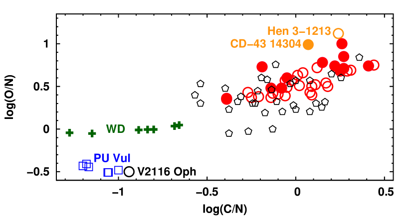
Figure 6: O/N versus C/N from the photospheric abundances. Current sample (filled circles) and sample from Paper III (open circles) compared with values from nebular lines (pentagons) and for PU Vul during outburst (squares). Crosses represent theoretical predictions for nova ejecta from CO WD with 0.65 M☉.

The two alpha elements measured here, titanium and oxygen, are important in understanding the formation and chemical evolution of Galactic populations. One route to studying the evolution of this pair of elements is to analyse their abundances relative to iron. Alpha elements and iron are produced in different ways. Alpha elements are created mostly by SNe II explosions of massive stars and consequently have a relatively short time-scale. Iron is created by SNe Ia that span much longer time-scales. The contamination of the interstellar medium by these two constituents leads to different chemical profiles for various populations. Separate sequences can be observed for distinct populations in diagrams constructed using the relative abundances of alpha elements and iron.

Fig. 7 presents relative abundances [O$/$Fe] and [Ti$/$Fe] as a function of metallicity ([Fe$/$H]) from our current (Table A1 in the online Appendix A) and previous samples of symbiotic giants. We also show values for stars of various stellar populations (halo, thin and thick disc and bulge) taken from a number of studies (see Paper III). The position of our objects in the [O$/$Fe] versus [Fe$/$H] diagram (Fig. 7 – top) indicates that most SySt are the members of Galactic disc. In the cases when [Fe$/$H] is close to $-0.8$ dex or smaller the extended thick-disc/halo population is suggested.

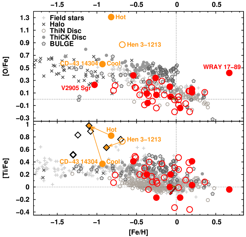
Figure 7: Top: oxygen relative to iron for various stellar populations with the positions of our targets denoted with large coloured circles (’filled’ for current sample and ’open’ from Paper III). For CD-43^∘14304 two cases are distinguished corresponding to solutions with different stellar parameters: ’Cool’ ($T_{\rm{eff}}$ = 3900 K) and ’Hot’ ($T_{\rm{eff}}$ = 4250 K). Four populations are distinguished: thin and thick discs, halo and bulge. Bottom: titanium relative to iron. Black open diamonds are giants in yellow symbiotic systems from Smith et al. (1996, 1997), Pereira et al. (1998) and Pereira & Roig (2009). Coloured arrows starting from the 0,0 point in the coordinates show shifts to our results applicable for the case with microtubulence velocity increased by +0.25 km s^-1 (red and yellow for the M-type and the yellow giants, respectively) according to the values given in the Table 5. See online edition for colour version.

In the [Ti$/$Fe] versus [Fe$/$H] plane (Fig. 7 – bottom) our M-type giants are grouped mostly at higher [Ti$/$Fe] in the region containing thick-disc and bulge stars. Each of our samples contains one yellow SySt, Hen 3-1213 from Paper III and CD-43^∘14304 from the current paper. These two stars show a small [Fe$/$H] and a large enhancement of [Ti$/$Fe] suggesting membership in the halo. Titanium and iron abundances have been published by other authors for both stars as well as for five other yellow symbiotics (Smith et al., 1996, AG Dra), (Smith et al., 1997, BD-21^∘3873), (Pereira et al., 1998, Hen 2-467), (Pereira & Roig, 2009, CD-43^∘14304, Hen 3-863, StH$\alpha$ 176 and Hen 3-1213). In all these cases, similar enhancement of [Ti/Fe] was found. Pereira & Roig (2009) also concluded that the overall abundance pattern of yellow SySt follows the halo abundances. The abundances obtained for Hen 3-1213 in our Paper III remain in good agreement with those of Pereira & Roig (2009). For CD-43^∘14304, Pereira & Roig (2009) obtained metal abundances based on optical spectra as follows: $\log{\epsilon(\mbox{Fe\,{\sc i}})}$ = 6.37 $\pm$ 0.19, $\log{\epsilon(\mbox{Ni\,{\sc i}})}$ = 5.05 $\pm$ 0.26 and $\log{\epsilon(\mbox{Ti\,{\sc i}})}$ = 4.81.

In our study, we adopted $T_{\rm{eff}}$ = 3900 K for CD-43^∘14304 corresponding to spectral type K7 according to the Mürset & Schmid (1999) classification and in agreement with the temperature derived from infrared colours (see Table 2). Taking into account fitting errors and uncertainties in atmospheric parameters the obtained iron abundance (6.54$\pm$0.10) remains in good agreement with that derived by Pereira & Roig (2009). However, Pereira & Roig (2009) adopted a 400 K warmer $T_{\rm{eff}}$, 4300 K. While the change in temperature does not significantly affect the resulted metallicity the derived titanium abundance (4.37$\pm$0.20) is much lower, shifting the position of this star in [Ti$/$Fe] versus [Fe$/$H] diagram into the region of stars characterized by typical compositions (Fig. 7 – bottom). As a check, we modelled CD-43^∘14304 with a hotter $T_{\rm{eff}}$, 4250 K, giving atmospheric parameters similar to those obtained by Pereira & Roig (2009): $T_{\rm{eff}}$ = 4300 K and $\log{g}$=+1.6. In this case, the iron abundance (6.65$\pm$0.09) also agrees and the titanium (4.93$\pm$0.20) is an almost perfect match to Pereira & Roig (2009). However, the resulting unusually high abundance of oxygen (9.18$\pm$0.24) would lead to very unrealistic ratio of [O$/$Fe] $\sim+1.3$ (Fig. 7 – top).

Pereira & Roig (2009) in their study determined the effective temperature using the classical technique of comparing neutral and ionized iron line abundances in optical spectra. The spectrum used for CD-43^∘14304 was obtained on 2007 August 26 (JD$\sim$2454339). According to ephemeris for eccentric orbit by Schmid et al. (1998), it corresponds to orbital phase $\sim$0.09. This phase is close to inferior spectroscopic conjunction with giant in the front. However, phase 0.09 is also soon after periastron passage when strengthened interactions between the binary members cause an increase in the nebular continuum that would strongly affect the depth of absorption lines. Indeed Gromadzki et al. (2013) observed periodic brightening in $V$ light curve in this system related to the periastron passage.

This example shows that considerable caution should be used when assigning effective temperatures to giants in SySt for chemical composition calculations. Abundances of some elements strongly depend on the temperature, as we have illustrated here for titanium and oxygen in hot, yellow giants (see Table 5). Previously (Paper III) we reported confirmation of high titanium abundances in yellow symbiotic systems and as well as a trend of increasing titanium with decreasing metallicity for both types of SySt, those with yellow and red M-type giants. In light of the example of CD-43^∘14304 this deserves additional study with temperatures reliably determined from infrared spectra. In at least some cases, the high titanium abundance could result from adopting an incorrectly high effective temperature.

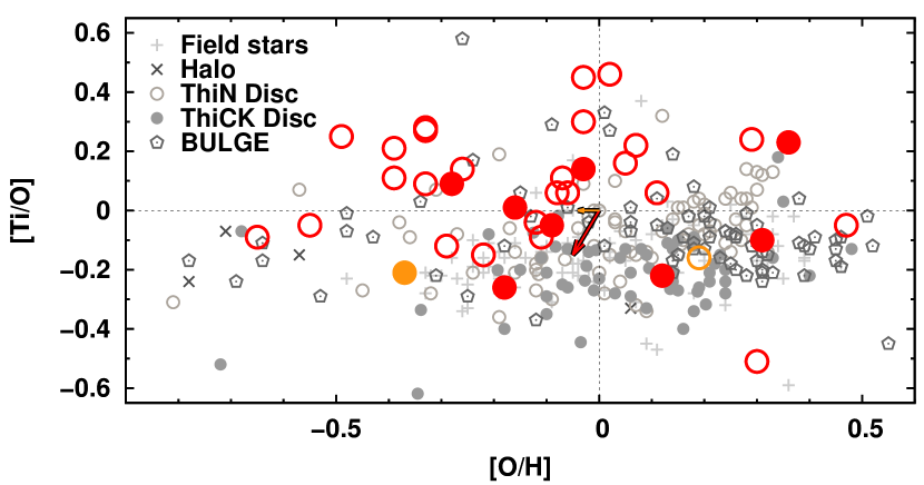
Figure 8: Titanium relative to oxygen for various stellar populations. Symbols analogous to those in Fig. 7.

In Fig. 8, the relative abundance of titanium to oxygen is presented. In this case the, vast majority of red giants are located at high [Ti$/$O] in a region mainly characteristic of the bulge population. Such increased titanium abundances are difficult to explain by theoretical models of nucleosynthesis in stellar interiors. A more reasonable explanation is that the microturbulent velocities used in our calculations, fixed on value 2 km s^-1 (see Section 3), are too small. In Fig. 7 and 8, the coloured arrows at the centre of the coordinates show shifts to obtained values that would result from the microturbulent velocity increased by +0.25 km s^-1, the estimated uncertainty in this parameter (Table 5). The use of increased microturbulence lowers the titanium overabundance observed in red symbiotic giants. We plan a further investigation into the microturbulence in the near future using a selected sample of systems with well-known absolute magnitudes.

Appendix A Relative abundances

Table 6: Selected relative abundances adopted for comparison with Galactic stellar populations (Figures 7 and 8).

Object	$[$O$/$Fe$]$	$[$Ti$/$Fe$]$	$[$Ti$/$O$]$	$[$Fe$/$H$]$	$[$O$/$H$]$
WRAY 15-1470	$+0.34$	–	–	$-0.26$	$+0.08$
Hen 3-1341	$+0.38$	$+0.41$	$+0.03$	$-0.54$	$-0.16$
WRAY 17-89	$+0.42$	$-0.04$	$-0.46$	$+0.67$	$+1.09$
V2416 Sgr	$+0.16$	$+0.41$	$+0.25$	$+0.20$	$+0.36$
V615 Sgr	$+0.04$	$+0.20$	$+0.16$	$-0.07$	$-0.03$
AS 281	$-0.06$	–	–	$-0.36$	$-0.42$
V2756 Sgr	$+0.20$	$+0.00$	$-0.20$	$-0.08$	$+0.12$
V2905 Sgr	$+0.23$	–	–	$-1.03$	$-0.80$
AR Pav	$+0.07$	$-0.17$	$-0.24$	$-0.26$	$-0.19$
V3804 Sgr	$-0.14$	$-0.17$	$-0.03$	$+0.05$	$-0.09$
V4018 Sgr	$+0.11$	$+0.03$	$-0.08$	$+0.20$	$+0.31$
V919 Sgr	$+0.09$	$+0.20$	$+0.11$	$-0.37$	$-0.28$
CD$-$43°14304	$+0.56$	$+0.37$	$-0.19$	$-0.93$	$-0.37$

Appendix B Spectra of all, 13 symbiotic giants, compared with synthetic fits

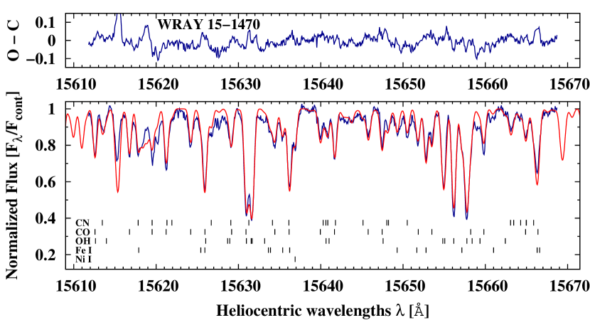
Figure 9: The spectrum of WRAY 15-1470 observed in 2010 May (blue line) and a synthetic spectrum (red line) calculated using the final abundances (Table 4).

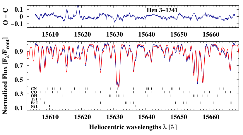
Figure 10: The spectrum of Hen 3-1341 observed in 2010 May (blue line) and a synthetic spectrum (red line) calculated using the final abundances (Table 4).

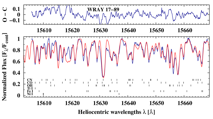
Figure 11: The spectrum of WRAY 17-89 observed in 2010 May (blue line) and a synthetic spectrum (red line) calculated using the final abundances (Table 4).

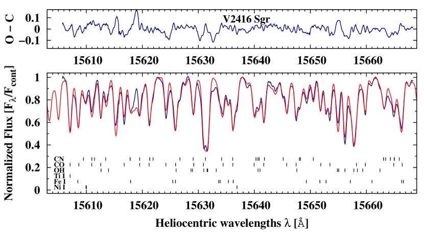
Figure 12: The spectrum of V2416 Sgr observed in 2010 June (blue line) and a synthetic spectrum (red line) calculated using the final abundances (Table 4).

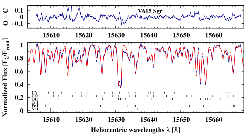
Figure 13: The spectrum of V615 Sgr observed in 2010 May (blue line) and a synthetic spectrum (red line) calculated using the final abundances (Table 4).

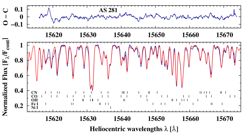
Figure 14: The spectrum of AS 281 observed in 2010 June (blue line) and a synthetic spectrum (red line) calculated using the final abundances (Table 4).

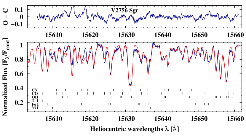
Figure 15: The spectrum of V2756 Sgr observed in 2010 June (blue line) and a synthetic spectrum (red line) calculated using the final abundances (Table 4).

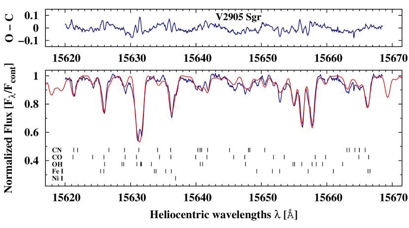
Figure 16: The spectrum of V2905 Sgr observed in 2010 June (blue line) and a synthetic spectrum (red line) calculated using the final abundances (Table 4).

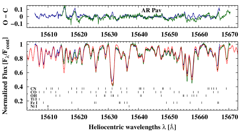
Figure 17: Spectra of AR Pav observed in 2009 June (blue line), 2010 May (green line), and a synthetic spectra (red continuous and dashed lines) calculated using the final abundances (Table 4).

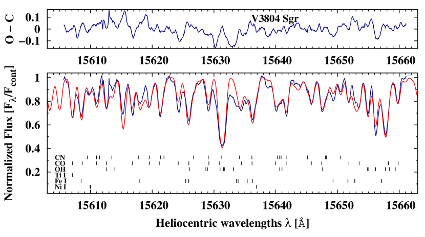
Figure 18: The spectrum of V3804 Sgr observed in 2009 August (blue line) and a synthetic spectrum (red line) calculated using the final abundances (Table 4).

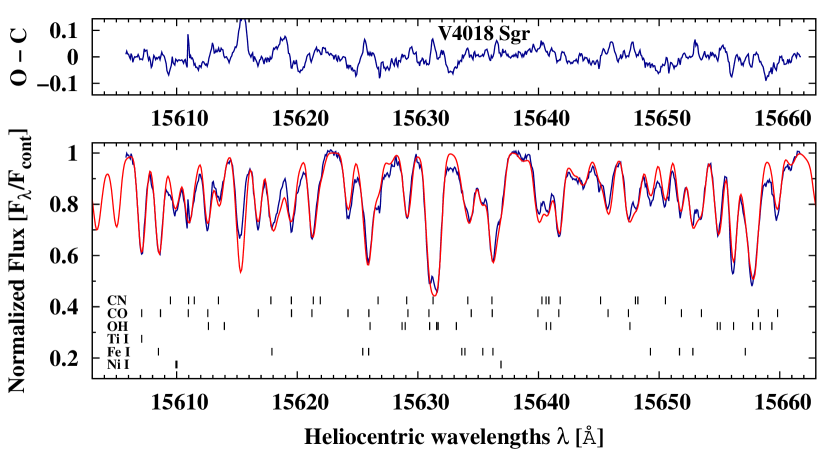
Figure 19: The spectrum of V4018 Sgr observed in 2010 June (blue line) and a synthetic spectrum (red line) calculated using the final abundances (Table 4).

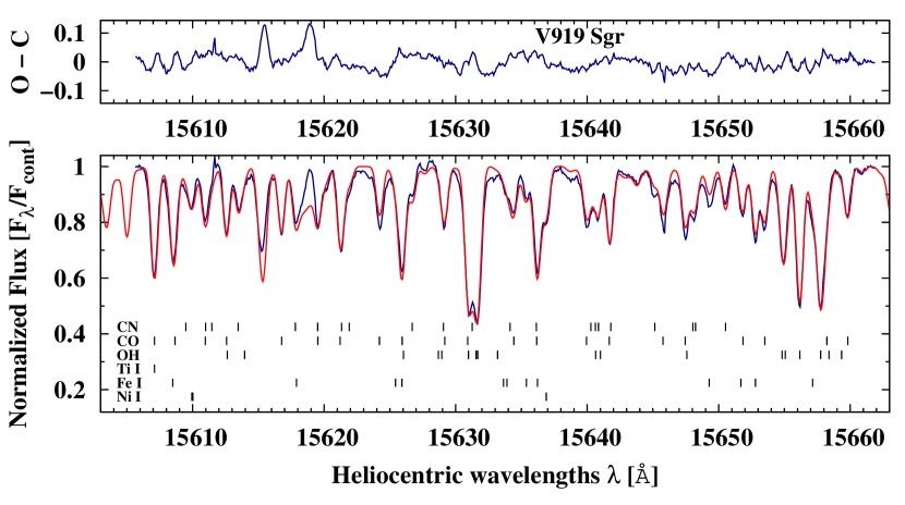
Figure 20: The spectrum of V919 Sgr observed in 2009 August (blue line) and a synthetic spectrum (red line) calculated using the final abundances (Table 4).

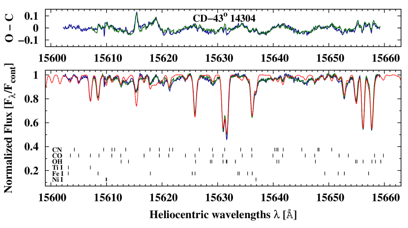
Figure 21: Spectra of CD$-$43°14304 observed in 2009 June (blue line), 2010 May (green line), and a synthetic spectra (red continuous and dashed lines) calculated using the final abundances (Table 4).

References

- Allen (1980) Allen D. A., 1980, MNRAS, 192, 521
- Asplund et al. (2009) Asplund M., Grevesse N., Sauval A., Scott P., 2009, ARA&A 47, 481
- Belczyński et al. (2000) Belczyński K., Mikołajewska J., Munari U., Ivison R. J., Friedjung M., 2000, A&AS, 146, 407
- Bessell & Brett (1988) Bessell M. S., Brett J. M., 1988, PASP, 100, 1134
- Brandt (1998) Brandt S., 1998, Data Analysis, Statistical and Computational Methods, Polish edn. Polish Scientific Publishers PWN, Warsaw
- Dumm & Schild (1998) Dumm T., Schild H., 1998, New Astron., 3,137
- Feast et al. (1990) Feast M. W., Whitelock P. A., Carter B. S., 1990, MNRAS, 247, 227
- Fitzpatrick (1993) Fitzpatrick M. J., 1993, in Hanisch R. J., Brissenden R. V. J., Barnes J., eds, ASP Conf. Ser. Vol. 52, Astronomical Data Analysis Software and Systems II. Astron. Soc. Pac., San Francisco, p. 472
- Gałan, Mikołajewska & Hinkle (2015) Gałan C., Mikołajewska J., Hinkle K. H., 2015, MNRAS, 447, 492 (Paper II)
- Gałan et al. (2016) Gałan C., Mikołajewska J., Hinkle K. H., Joyce R. R., 2016, MNRAS, 455, 1282 (Paper III)
- Goorvitch (1994) Goorvitch D., 1994, ApJS, 95, 535
- Gromadzki et al. (2013) Gromadzki M., Mikołajewska J., Soszyński I., 2013, Acta Astron., 63, 405
- Gustafsson et al. (2008) Gustafsson B., Edvardsson B., Eriksson K., Jørgensen U. G., Nordlund Å, Plez B., 2008, A&A, 486, 951
- Joyce (1992) Joyce R., 1992, in Howell S., ed., ASP Conf. Ser. Vol. 23, Astronomical CCD Observing and Reduction Techniques. Astron. Soc. Pac., San Francisco, p. 258
- Kovetz & Prialnik (1997) Kovetz A., Prialnik D., 1997, ApJ, 477, 356
- Kucinskas et al. (2005) Kucinskas A., Hauschildt P. H., Ludwig H.-G., Brott I., Vansevičius V., Lindegren L., Tanabé T., Allard F., 2005, A&A, 442, 281
- Kurucz (1999) Kurucz R. L., 1999, available at: http://kurucz.harvard.edu
- Medina Tanco & Steiner (1995) Medina Tanco G. A., Steiner J. E., 1995, AJ, 109, 1770
- Mélendez & Barbuy (1999) Mélendez J., Barbuy B., 1999, ApJS, 124, 527
- Mikołajewska et al. (1997) Mikołajewska J., Acker A., Stenholm B., 1997, A&A, 327, 191
- Mikołajewska (2003) Mikołajewska J., 2003, in Corradi R. L. M., Mikołajewska J., Mahoney T. J., eds, ASP Conf. Ser. Vol. 303, Symboitic Stars Probing Steller Evolution. Astron. Soc. Pac., San Francisco, p. 9
- Mikołajewska, Ivison & Omont (2003) Mikołajewska J., Ivison R. J., Omont A., 2003, in Corradi R. L. M., Mikołajewska J., Mahoney T. J., eds, ASP Conf. Ser. Vol. 303, Symboitic Stars Probing Steller Evolution. Astron. Soc. Pac., San Francisco, p. 478
- Mikołajewska (2012) Mikołajewska J., 2012, Balt. Astron., 21, 5
- Mikołajewska et al. (2014) Mikołajewska J., Gałan C., Hinkle K. H., Gromadzki M., Schmidt M. R., 2014, MNRAS, 440, 3016 (Paper I)
- Mürset & Schmid (1999) Mürset U., Schmid H. M., 1999, A&AS, 137, 473
- Nussbaumer et al. (1988) Nussbaumer H., Schild H., Schmid H. M., Vogel M., 1988, A&A, 198, 179
- Pereira (1995) Pereira C. B., 1995, A&AS, 111, 471
- Pereira et al. (1998) Pereira C. B., Smith V. V., Cunha K., 1998, AJ, 116, 1977
- Pereira & Roig (2009) Pereira C. B., Roig F., 2009, AJ, 137, 118
- Phillips (2007) Phillips J. P., 2007, MNRAS, 376, 1120
- Podsiadlowski & Mohamed (2007) Podsiadlowski Ph., Mohamed S., 2007, Balt. Astron., 16, 26
- Quiroga et al. (2002) Quiroga C., Mikołajewska J., Brandi E., Ferrer O., García L., 2002, A&A, 387, 139
- Richichi et al. (1999) Richichi A., Fabbroni L., Ragland S., Scholz M., 1999, A&A, 344, 511
- Rutkowski et al. (2007) Rutkowski A., Mikołajewska J., Whitelock P. A., 2007, Balt. Astron., 16, 49
- Schild et al. (2001) Schild H., Dumm T., Mürset U., Nussbaumer H., Schmid H. M., Schmutz W., 2001, A&A, 366, 972
- Schlafly & Finkbeiner (2011) Schlafly E. F., Finkbeiner D. P., 2011, ApJ, 737, 103
- Schlegel, Finkbeiner & Davis (1998) Schlegel D. J., Finkbeiner D. P., Davis M., 1998, ApJ, 500, 525
- Schmid & Schild (1990) Schmid H. M., Schild H., 1990, MNRAS, 246, 84
- Schmid et al. (1998) Schmid H. M., Dumm T., Mürset U., Nussbaumer H., Schild H., Schmutz W., 1998, A&A, 329, 986
- Schmidt et al. (2006) Schmidt M. R., Začs L., Mikołajewska J., Hinkle K. H., 2006, A&A, 446, 603
- Schulte-Ladbeck (1988) Schulte-Ladbeck R. E., 1988, A&A, 189, 97
- Scott et al. (2015) Scott P., Asplund M., Grevesse N., Bergemann M., Sauval A. J., 2015, A&A, 573, 26
- Smith et al. (1996) Smith V. V., Cunha K., Jorissen A., Boffin H. M. J., 1996, A&A, 315, 179
- Smith et al. (1997) Smith V. V., Cunha K., Jorissen A., Boffin H. M. J., 1997, A&A, 324, 97
- Sneden et al. (2014) Sneden C., Lucatello S., Ram R. S., Brooke J. S. A., Bernath P., 2014, ApJS, 214, 26
- Van Belle et al. (1999) Van Belle G. T. et al., 1999, AJ, 117, 521
- Vogel & Nussbaumer (1992) Vogel M., Nussbaumer H., 1992, A&A, 259, 525