Efficient Sampling for Better OSN Data Provisioning

Abstract

Data concerning the users and usage of Online Social Networks (OSNs) has become available externally, from public resources (e.g., user profiles), participation in OSNs (e.g., establishing relationships and recording transactions such as user updates) and APIs of the OSN provider (such as the Twitter API). APIs let OSN providers monetize the release of data while helping control measurement load, e.g. by providing samples with different cost-granularity tradeoffs. To date, this approach has been more suited to releasing transactional data, with graphical data still being obtained by resource intensive methods such a graph crawling. In this paper, we propose a method for OSNs to provide samples of the user graph of tunable size, in non-intersecting increments, with sample selection that can be weighted to enhance accuracy when estimating different features of the graph.

I Introduction

Online Social Networks (OSNs) continue to grow rapidly with 1.7 billion monthly active users on Facebook and over 300 million on Twitter. OSN providers are making small portions of their vast data collections available to different external parties, including researchers, based on business considerations (increasing reach and sales or enabling external application writers). The manner of providing access, the choice of the samples, etc., are all unilateral decisions made by the OSN providers. In this paper, we argue that there are better ways to make samples of user data available to external parties that would benefit all. We examine current practices in OSN data availability, the manner of analyses which use the data, and the challenges posed by scale and statistical features of the data itself. We propose sampling schemes that accommodate the need estimate accurately in multiple data dimensions and can also serve different sampling rates without duplication under a controllable database load.

We examine current practices in OSN data availability, the manner of analyses which use the data, and the challenges posed by scale and statistical features of the data itself. Externally to OSNs there is much interest in understanding users, their OSN relationships, and the OSN events they generate. Research aims to understand statistical properties, such as connectivity, clustering, node degree, events. Increasingly, there is commercial interest in identifying specific subsets of the OSN graph (active users, highly connected and influential users, groups of users with specific common interests) and subsets of OSN events, including updates containing specific keywords, such as a company name, product, or service.

I-A Current trends and our motivation

There are currently two types of methods to obtain information concerning OSN networks. The first is direct measurement of eternally visible portions of the OSN, possibly as a member, (e.g., viewing accessible portions of users’ profile pages, or registering for content updates). The second is by employing tools provided by the OSN, such as the Twitter API, that give partial visibility into users relationships, and the stream events (status updates, i.e. tweets). Much research activity (see Section II) has focused both on developing strategies for efficiently using these resources and estimating OSN properties from the subsets of data so obtained. This approach often involves traversal of portions of the OSN graph, en passant compiling relatively large data subsets for research and evaluation purposes. However, such approaches are relatively costly in time, resources, and expertise, and hence not feasible for non-specialist use.

A more effective model for non-specialist users positions them at the end of a chain of commercial relationships. The chain starts with OSNs monetizing access to their user data by providing partial data feeds with members selected, e.g., by sampling or attribute-based filtering, potentially at different price points depending on factors such as the sampling rate and reported detail per item. Independent OSN analytic services subscribe to these data feeds, possibly joining them with OSN data measured independently, and other data sources such as demographic information. This provides downstream feeds and/or query functionality that can be sold to non-specialist end users. The OSN analytic services would subscribe to higher-cost data feeds than would be economical for an individual user, with the costs effectively being divided over the set of end users.

In order to realize the model just described, what is needed is a systematic way for OSNs to release samples of graph level objects—such as users (nodes), relationships between users (links) and node clusters—with a level of sampling that can be tuned to a desired price point. OSNs primarily benefit in two ways. First, this produces a new data feed that can be monetized. Second, this reduces the measurement based load on the OSN service network, since it provides information that would otherwise be obtained only by direct measurement of the OSN. A corollary of this second point it that OSNs have an incentive to employ a sampling strategy that, for a given data feed sampling rate optimizes the accuracy of analyses built on the feed. This reduces any incentive for subscribers to revert to independent measurement.

How should the OSN sample its user graph? The constraints for external measurement do not apply to the OSN provider. We assume that the OSN stores the user graph in a database and that it is feasible to pass exhaustively over all elementary graph objects (nodes and links) in order to compile samples. Composite objects such as node clusters of a given size may also be amenable to treatment. Within this framework, a sampling methodology should exhibit the following three properties:

S1

Multidimensional Estimation Accuracy: There are many interesting properties for OSN analytics, including node properties (e.g., event activity rate, node in and out degree) and link properties (e.g., degree pairs of connected nodes). The sampling methodology must be able to yield accurate estimates of the marginal distributions of the variables, e.g., to service queries on the distribution of the number of connection beween OSN users. However for OSN analytics, there is a great interest in understanding the relationships between user properties, as expressed through queries such as finding the proportion of all connections or of all event activity that is represented by a given proportion of the most connected users (see e.g. [14]). Answering such queries requires accurate estimation of not only the joint distribution of the variables concerned, but the joint mass distributions, i.e., the joint distributions weighted by the values of one of more variables.

S2

Single Pass Serving of Different Sampling Rates: rather than have separate database passes for each sampling rate with associated duplication of resource usage, we wish to serve queries based on any sampling rate from a single pass through the data.

S3

Control of User Database Access Rate: We assume that in order to limit measurement access load on the database, the access rate must be controlled to a desired level. This may occur through limiting either the frequency of exhaustive passes, or the frequency of individual accesses during the traversal.

A challenge for creating a sampling regime satisfying these properties comes from certain empirical facts: (i) the distributions of some variables are markedly skewed, exhibiting heavy tails, and (ii) there are strong correlations between some pairs of variables (see Section V). Uniform sampling is effective for estimating ordinary distributions, but is a poor choice for estimating the mass distribution of a heavy-tailed variable [5], since random omission from the sample of a single large value can render estimates inaccurate. Instead, weighted sampling (see e.g., [9]) can be used to preferentially sample high-weight objects to provide accurate estimates of mass distributions.

I-B Contribution and Outline

The contribution of this paper is first to specify a sampling methodology that satisfies the properties [S1,2,3] above. We propose to meet the condition [S1] by compiling, for each type of graph object (e.g., node, link) a uniform sample and one or more weighted sample sets. This raises two questions. First: how should the weightings be chosen? A minimal way to do this is to determine the smallest set of (roughly) independent heavy-tailed variables of interest, and use each of these as a weight. In this approach, correlations between variables are advantages in the sense that they may reduce the number of sample sets that must be compiled. The second question is which sample set or sets should be used in serving a given query. We propose that the uniform sample be used for ordinary distribution queries and queries concerning the mass distribution of light-tailed variables, while a query concerning the mass distribution of a heavy-tailed variable should use a weighted sample set of either that variable, or, if absent, a sample set weighted by a correlated heavy-tailed variable.

We propose to meet condition [S2] by using Priority Sampling[9] to compile, for each graph element type and sample weighting, a Master Sample comprising a randomly ordered subset of graph elements. A simple query on the master sample returns the first $k$ items in order, with possible followup queries returning the next $k$ and so on. A more complex query returns only elements that match a given predicate. Here, the parameter $k$ determines the effective sampling rate.

Priority Sampling can be implemented as either an offline or a streaming algorithm. Correspondingly, condition [S3] can be achieved by limiting a frequency of an offline redrawing of the sample sets or by streaming graph elements into the sampler at some desired rate.

The outline of the paper is as follows. Section II surveys the current state of related work and positions our contribution with respect to this. Section III describes some classes of query used in OSN analysis and discuss the ramifications for observed distribution features. Section IV describes the compilation of master samples using Priority Sampling, and procedures for estimating weight sums over subsets of population elements specified by a selection predicate. We also show how to estimate both ordinary and mass distributions from the samples. For evaluation purposes we collected an OSN dataset described in Section V; the evaluations are described in Section VI. Our concluding discussion in Section VII sketches some possible extensions of our approach.

II A Survey of OSN Measurement

In this section we survey the current state of external and internal measurement of OSN and node and link-level queries of common interest. We describe the known effects of sampling on query accuracy and the challenge that heavy-tailed distributions of the variable bring to answering queries. We also explain how our work develops the state-of-the-art in distribution estimation and sample provisioning.

II-A External Measurements, Crawling and Random Walks

There is a large literature on external measurements of OSNs that illustrates the scale and complexity involved in data acquisition. Early papers gathered data by crawling Orkut [20] and Twitter [16, 14]. A more recent, larger scale study [18] used 20 machines simultaneously sending a large number of requests to Twitter to fetch nearly 42 Million user profiles and over 100 Million tweets. Another [4] fetched nearly 55 Million user profiles, 2 billion follow links, and 1.75 billion tweets.

The statistical properties of OSN data acquisition through crawling has been examined in the framework of random walks on graphs. The general theory of these goes back to [10]. A number of different sampling strategies for graph traversal have been proposed, and evaluated for online networks including the web, peer-to-peer, and social networks. These evaluations have included examining the dependence of various graphical statistics on the sampling rate. Unbiased sampling via Metropolis-Hastings Random Walks was examined in Facebook [12] and P2P networks [23]. Forest Fire Sampling [19] explores the graph in a Markovian walk from randomly selected nodes, while Frontier Sampling [21] used multidimensional random walks to mitigate trapping. Weighted random walks on graphs to implement stratified sampling was proposed in [17]. Graph sampling methods exploiting temporal clustering properties of OSN updates are presented in [1]. Estimation of YouTube video counts through random prefix sampling was proposed in [30]. Estimating degree distribution under network sampling is treated as a linear inversion problem by [29].

The effectiveness of different crawling and non-crawling sampling strategies have been compared though their effects on estimation of graphical statistics. Uniform sampling, BFS with threshold and OPIC (online page importance) were compared in [3]. The effects of different sampling strategies information diffusion metrics in Twitter were examined in  [6]. Sampling based estimates of the distributions of popularity, length & number of views reported in YouTube video metadata were compared in [15]. Our work is distinct from these in that we consider the methodological underpinnings of what makes an effective sampling strategy and its relation to the queries that are served.

II-B OSN Queries and Feature Distributions

OSN research literature has focused on some popular questions about various properties. These include characterization concerns such as statistics about “friendships” (which in asymmetric OSNs like Twitter includes notions of following and followers), outliers, connected and disconnected components in the social graph, degree of separation, homophily, assortativity, and participation fraction [3]. Dynamic properties such as reach, spread, and cascade focus on users and applications that have higher influence, as characterized by the speed with which an application or a user’s communication spreads [6]. This topic is of considerable commercial interest.

The joint distributions of graphical statistics in online networks are of great interest for the user community [24] and have been studied experimentally by a number of authors. The joint distributions of OSN user characteristics (numbers of friends, followers, activity measures such as number of posts) were studied in [14]. [20] found correlations between in and out degrees in crawls of Flickr, Orkut and YouTube. [4] studied the dependence between different measures of influence in Twitter, namely, in-degree, retweets and mentions. Our work is different from these in that we provide insight on how best to sample based on the desired target statistics. Closer to our approach is [27], which proposed Probability Proportional to Size sampling in OSN for estimation of node degrees. Our work goes further: we consider the problem of how to estimate for joint distributions of interest in applications. None of the above works consider our problem of how to play out samples for analysis in a optimal, tunable, and scaleable manner.

OSNs place various constraints on the ability of users to obtain social graph data. Twitter provides limited live samples via their Streaming API, while the Search API allows queries against recent or popular tweets [26]. Facebook limits the number of API queries that can be submitted in a time period. Thus, most of the research described here reports on a sample of the data, which leads to questions about the nature and size of samples needed to answer specific questions. The evolution of this data, including the effective sampling rates, has been studied over a multi-year period by [28], which also notes the inherent activity bias of this datasets. Even studies that report on full crawls could be out of date after a relatively short period of time.

II-C The Challenge of Heavy Tails

The approach of this paper builds on experience and methods from sampling Internet traffic flow records. The distribution of bytes per flow is heavy-tailed [11]. Consequently, uniform sampling of flows, while providing good estimates of counts of flows satisfying any predicate, provides bad estimates of their byte counts because non-selection of large flows greatly impact byte estimation accuracy. On the other hand, weighting sampling by byte size enables accurate estimation of bytes in flows satisfying any predicate, resulting in bad estimates of flow counts. The conclusion here is that the heavy-tailed byte distribution makes it difficult to simultaneously satisfy the accuracy requirements of byte and flow estimation in a single sample. Instead, it is best to compile two sample reservoirs, one with uniform sampling to serve flow-level queries, one with bytes weighted sampling to serve byte-level queries [8]. In this paper we will exploit existing methods for efficient Probability Proportional to Size sampling [9, 2], but the application of these to the problem of scaleable playout of samples without repetition is new.

III Modeling OSN Queries

Our work focuses on queries based on topological features of single node or pairs of nodes, and on activity features. We consider the class of queries that correspond to statements concerning the (possibly joint) distribution of these node quantities, or some summary statistic that integrates over the distributions. Thus, our evaluation focuses on the question of how accurately the distributions of these features can be estimated from the collection of sampling reservoirs. Many distributional queries and features of commercial interest (see [14, 24]) can be abstracted into forms that we now describe.

The set of single-user queries include:

• Distributions of single features, e.g., given $n$ find $x$ such that $x\%$ of users generate at least $n$ tweets each.

• Self-weighted mass distributions of single features, e.g., given $y$, find $x$ such that the top $x\%$ most active users generate $y\%$ of all tweets.

• Mass distributions of one feature weighted by another, e.g., given $y$, find $x$ such that the top $x\%$ most followed users together generate $y\%$ of all tweets.

In this paper we will focus on single use queries of the form just described. However, the same methods can, in principle, be applied to pair user queries including the following:

• Joint distributions of features from two users, e.g., given $y$, find $x$ such that $x\%$ of the total activity between user pairs are between the top $y\%$ most active users.

• Pairwise summary statistics such as assortativity, i.e., the correlation between graph degrees of directly connected users.

IV Samples, Playout & Estimation

This section describes the technical approach underpinning our work. Section IV-A motivates weighted sampling as a response to heavy-tailed distributions of node characteristics, while Section IV-B illustrates the ramifications of correlations between different heavy-tailed variables for sampling. Section IV-C briefly reviews Priority Sampling, while Section IV-D describes how it can be used to fulfill the objectives S1–3 in the introduction. Section IV-E shows how samples selected through these means can be used to estimate the mass distributions described in Section III.

IV-A Heavy Tails and Weighted Sampling

Our approach to sampling is guided by the principle that sampling methodology should be chosen to match the statistical characteristics of the data with the queries on that data. In this case, the salient statistical features are:

• Node features such as graph degree and activity that exhibit highly skewed, heavy-tailed distributions.

• Node characteristics that exhibit varying amounts of statistical correlation; see [14] and Section VI.

Uniform sampling estimates mass distributions poorly in case (i), since estimation accuracy of large sizes becomes highly sensitive to inclusion or exclusion from the sample of large items, i.e., those for which the measure of interest, such as node degree, is large. Weighted sampling reduces estimation variance by boosting the relative selection probabilities of large items relative to small items. The prime example is selecting a item of size $x$ with Proportional to Size (PPS). A number of variants of this approach exist, including weighted sampling without replacement, Priority Sampling [9], and Variance Optimal Sampling [7]. All these methods are able to construct a sample of a specified fixed size. Priority Sampling and Variance Optimal sampling have efficient implementations on data streams, and the latter minimizes estimation variance compared with any online or offline unbiased estimator.

IV-B Correlated Heavy Tails: A Thought Experiment

Consider two families $X=\{X_{i},\ i=1,\ldots,n\}$ and $Y=\{Y_{i},\ i=1,\ldots,n\}$ of heavy-tailed random weights, drawn independently within each family. How do correlations between $X$ and $Y$ affect PPS sampling? We use the following thought experiment to examine two extreme cases:

• Perfect correlation: $X_{i}=Y_{i}$ for all $i$;

• Independence: $X_{i}$ and $Y_{i}$ are independent for all $i$.

Under perfect correlations, PPS sampling using $X_{i}$ as weights is effective for estimating large $Y_{i}$, since these equal the corresponding $X_{i}$. But when $X$ and $Y$ are independent, the occurrences of large values of $X$ and $Y$ are not correlated, so weighted sampling based on $X$ will not select larger $Y$. In practice, correlations between node variables lie between these extremes. Our experiments in Section VI find varying degrees of correlation between different heavy-tailed node variables. The less strongly correlated variables are not interchangeable as weights for PPS sampling.

IV-C Priority Sampling

The specific form of weighted sampling we use in the paper is Priority Sampling [9]. From a population $\Omega$ of items with weights $w_{i}$, Priority Sampling constructs a sample of any fixed size $k$ as follows. First generate for each $i$ a priority $\alpha_{i}=w_{i}/u_{i}$ where each $u_{i}$ is independently and uniformly distributed in $(0,1]$. Then $\Omega(k)$ comprises $k$ items of highest priority. Define the threshold $z(k)$ as the $(k+1)^{\textrm{st}}$ highest priority. Then the effective sampling probability is is $p_{i}(w_{i},k)=\min\{1,w_{i}/z(k)\}$, and using the Horvitz-Thompson inverse probability method [13],

$$\widehat{w}_{i}=\left\{\begin{array}[]{ll}\max\{w_{i},z(k)\}&\mbox{ if $i$ is sampled}\\ 0&\mbox{ if $i$ not sampled}\\ \end{array}\right.$$ (1)

is an unbiased estimator of $w_{i}$ [9]. An unbiased estimate of the subset sum $X(S)=\sum_{i\in X}x_{i}$ over any subset $S$ is just $\widehat{X}(S)=\sum_{i\in S}\widehat{x}_{i}$. A common case is when $S$ is a set of items satisfying a predicate (e.g., users registered in some region or with at least some number of relationships).

IV-D Database Sampling and Playout

In this section we show how Priority Sampling is well suited to serve database queries based on any predicate with a mechanism possessing the following properties

• Different sample sizes and predicates can be served from a master sample.

• Multiple non-overlapping samples can be generated on the same predicate.

• Sample volume or processing load can be controlled.

In each case, unbiased estimators can be constructed from the corresponding samples.

IV-D1 Creation of the Master Sample

Following [2], we first create the master sample: a descending priority-order sorted version $\Omega^{\prime}$ of the population $\Omega$ of database records, typically realized a sorted index into the original set. This prodecure is performed one-time only: all randomness occurs during this initial step. If the size of the master sample must be constrained to a size $k_{\mathrm{max}}$, we take as $\Omega^{\prime}$ the $k_{\mathrm{max}}$ elements of largest priority.

IV-D2 Samples of Given Size Over a Predicate

A sample $S(k)$ of size $k$ over any predicate $S$ and $k$ can be constructed by selecting the first $k$ items in $\Omega^{\prime}$ that match the predicate. These are returned along with the sampling weights $w_{i}$ and the sampling threshold $z(S,k)$ being the $(k+1)^{\textrm{s}t}$ largest priority of items matching $k$. If $\Omega^{\prime}$ is exhausted with only $1+k^{\prime}$ matching items found, then the first $k^{\prime}$ of these are returned, along with $z(S,k^{\prime})$.

IV-D3 Non-overlapping Samples on a Given Predicate

An initial sample $S(k)$ can be extended to size $k+j$ by adjoining the next $j$ elements that match $S$, to yield $S(j+k)$. The original $z(S,k)$ is discarded and $z(S,j+k)$ used for estimation purposes. This step can be repeated as required; exhaustion of $\Omega^{\prime}$ is handled as above.

IV-D4 Control of Computational Cost

Computational cost may be controlled instead by selecting elements matching $S$ from within the first $k$ of all elements of $\Omega^{\prime}$. In this case, the threshold reported is $z(k)$, the $(k+1)^{\textrm{s}t}$ largest priority in all of $\Omega^{\prime}$.

IV-D5 Estimation Accuracy

General bounds for estimation accuracy of subset sums has been determined in [25]: an unbiased estimate $\widehat{X}$ of a subset sum $X$ based in $k$ samples obeys the bound $\mathrm{var}(\widehat{X})\leq\sqrt{X/(k-1)}$.

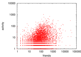
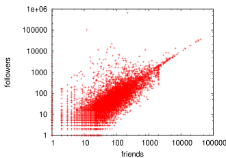
Figure 1: Pairwise scatter plots of node characteristics of 10,000 random users. Left: weaker correlation, $r_{s}(\textsc{ac},\textsc{fr})=0.44$. Right stronger correlation $r_{s}(\textsc{fo},\textsc{fr})=0.82$ (Statistics from full dataset).

IV-E Distribution Estimation

We now show how the joint distributions of user variables used in the queries described in Section III can be computed using subset sums whose estimation from samples is described above in Sections IV-C and IV-D. We model each user record in the database as containing a set of $m$ features $(x^{(1)},\ldots,x^{(m)})$. A sampling weight is a value $w=w(x^{(1)},\ldots,x^{(m)})$ computed as a function of its fields. These value may be directly reported in the record, and/or in the simplest case be a single feature.

Given a predicate $\pi$, we will denote

$$\widehat{X}^{(j)}(w,k,\pi)=\sum_{\pi(i)\wedge i\in\Omega(k)}x^{(j)}_{i}/p_{i}(w_{i},k)$$ (2)

the estimate of the subpopulation sum of $x^{(j)}$ over all records satisfying the predicate $\pi$, based on a sample of size $k$ using weights $w_{i}=w(x_{i}^{(1)},\ldots,x_{i}^{(m)})$. We also distinguish the estimated subpopulation count:

$$\widehat{N}(w,k,\pi)=\sum_{\pi(i)\wedge i\in\Omega(k)}1/p_{i}(w_{i},k)$$ (3)

We will omit the $\pi$ when all records are to be used, corresponding to the case $\pi$ is identically true.

• Distribution of $X^{(j)}$. This estimate aims to yield statements of the form: a proportion $q$ have records have $X^{(j)}$ less than or equal to $y$. Given a value $y$, define

  $$q(y)=\frac{\widehat{N}^{(j)}(w,k,x^{(j)}\leq y)}{\widehat{N}^{(j)}(w,k)}$$ (4)

  Then $y$ estimates the $q(y)$-quantile of $X^{(j)}$. To estimate the full CDF of $X^{(j)}$ we use the value $q(y)$ as $y$ is varied. We denote by $\widehat{D}_{w}(X^{(j)})$ the resulting distribution estimate.

• Mass distribution $X^{(\ell)}$ by quantiles of $X^{(j)}$. This estimate aims to yield statements of the form: a proportion $r$ of the total mass of $X^{(\ell)}$ is contained in a proportion $q$ of records with smallest $X^{(j)}$. Given a value $y$, define

  $$q(y)=\frac{\widehat{N}(w,k,x^{(j)}\leq y)}{\widehat{N}(w,k)},\quad r(y)=\frac{\widehat{X}^{(\ell)}(w,k,x^{(j)}\leq y)}{\widehat{X}^{(\ell)}(w,k)}$$ (5)

  Similar to above, $y$ estimates the $q(y)$-quantile of $X^{(j)}$, while $r(y)$ is the proportion of the mass of $X^{(\ell)}$ attributable to records with $X^{(j)}$ no greater than this quantile $y$. Varying $y$ as a parameter yields the estimated curve $(q(y),r(y))$ of the mass distribution of $X^{(\ell)}$ by the quantiles of $X^{(j)}$. $\widehat{M}_{w}(X^{(\ell)},X^{(j)})$ is the resulting mass distribution estimate.

Note that in all the above examples, one can further restrict the distribution to those items matching additional predicates that select on the $(x^{(1)},\ldots,x^{(m)})$.

V OSN Measurement Dataset

This section describes the acquisition and properties of the OSN dataset used in the measurement-based study of this paper. Twitter supplies streamed data on a sampled basis via its Streaming API interface [26], also referred to as the gardenhose. This provided a sample of 5 public tweets out of every 100 (based on the last two digits of the monotonically increasing status IDs), written on a single TCP connection, significantly minimizing overhead on Twitter servers. Twitter guaranteed randomness via their selection process and their internal algorithm for assigning status IDs. Each record streamed included nearly forty fields ranging from information about the user who generated the tweet (including number of friends, followers, status IDs) to information about the tweet itself (textual content, language, etc.). During 2010, we gathered seven consecutive weeks of data resulting in 75 million tweets and the associated information generated by just over 8 million unique users. We selected 100,000 unique users using weighted sampling with each user weighted proportionally to the number of tweets that the user originated in our sample. Through the Twitter API we obtained the list of their friends and followers.

Our dataset is inherently activity weighted since the more active users have a greater chance of selection than the less active users; see [28]. Thus, the distributions of node variables in our data is different from those in the unsampled user database available to an OSN provider. However, this does not change the essential thrust of our work (how best to sample from correlated heavy-tailed distributions) since the heavy-tails we observe are not created by sampling.

In graph language, each node corresponds to a user, and we denote by fo and fr the numbers of followers and friends as reported in the most recently observed status update for each node. The activity ac is the number of status updates observed for a given user. Each of the 7.3 million direct graph links $(u_{1},u_{2})$ corresponds to a follower relationship, i.e., $u_{2}$ is a follower of $u_{1}$. An example of a link feature combining features from both nodes is ffan, the follower fanout of a link $(u_{1},u_{2})$, defined as the ratio $\textsc{fo}(u_{2})/\textsc{fo}(u_{1})$. We believe this is an interesting feature because high values of ffan indicate links where a tweet for user $u_{1}$ has the potential to be amplified if retweeted by user $u_{2}$, since $u_{2}$ has a larger follower set.

As stated in Section I, the correlations amongst different data features have ramifications for the choice of a set of different sample weightings. If a set of variables is strongly mutually correlated, then a sample weighting based on any one of them may be sufficient for estimating the mass distribution of any of them. To assess the correlation amongst user features, we calculated the Spearman rank correlation $r_{s}$ between each pair of features to normalize the varying scaling behavior of the features. fr and fo are strongly correlated, with $r_{s}(\textsc{fr},\textsc{fo})=0.82$. Their correlation with ac is weaker: $r_{s}(\textsc{ac},\textsc{fo})=0.53$ and $r_{s}(\textsc{ac},\textsc{fr})=0.44$.

We also use scatter plots of pairs of user features to illuminate the relationships between the variables, using a uniform random sample of 10,000 users; see Figure 1. High values of fr and ac are relatively uncorrelated, while high values of fo and fr are more strongly correlated. The consequences of this behavior are discussed next.

VI Measurement Study & Evaluation

We show how the estimation accuracy of both ordinary and mass distributions depends both on the variables whose distribution is to be estimated and the features used to weight sampling. To assess accuracy we compare the estimated ordinary and mass distributions $D_{w}(X)$ and $M_{w}(X,X^{\prime})$ of $X$ (according to the quantiles of $X^{\prime}$ in the mass case), under the sample weighting $w$, with the true distributions computed as “estimates” of all the data instead of sampling. For node variables, we estimated the ordinary distributions $\widehat{D}_{w}(X)$ where $X\in\{\textsc{fo},\textsc{fr},\textsc{ac}\}$ and different weighting schemes $w\in W=\{\textsc{uni},\textsc{fo},\textsc{fr},\textsc{ac}\}$ where uni is uniform sampling and other $w$ denote weighting by the specified node variable. The mass distribution estimates were $\widehat{M}_{w}(X,X^{\prime})$ used $X,X^{\prime}\in\{\textsc{fo},\textsc{fr},\textsc{ac}\}$ and $w\in W$. For the link variable ffan, we estimate the ordinary distribution using $\widehat{D}_{w}(\textsc{ffan})$ with $w\in W^{\prime}=\{\textsc{uni},\textsc{fo}_{1},\textsc{fo}_{2},\textsc{ffan}\}$ where for $i\in\{1,2\}$, $\textsc{fo}_{i}$ is the fo value of node $u_{i}$ in a directed follower link $(u_{1},u_{2})$. We estimated the mass distributions $M_{w}(\textsc{ffan},X^{\prime})$ for $X^{\prime}\in\{\textsc{fo}_{1},\textsc{fo}_{2},\textsc{ffan}\}$ and $w\in W^{\prime}$.

Our principle comparison was between true and estimated distribution, the difference characterized by the maximum absolute difference of the cumulative distributions, similar to the Kolomogorov-Smirnov (KS) test statistic [22]. For each $w,X$ (and $X^{\prime}$ in the mass case) we conducted 100 independent selections of 1000 samples, and summarized differences using the median KS statistic over the selections.

w	X=fo	X =fr	X = ac
uni	0.066	0.052	0.352
fr	0.130	0.152	0.330
fo	0.116	0.110	0.346
ac	0.069	0.055	0.347

TABLE I: Ordinary Distribution Accuracy for Node Variables: Median KS statistic for $D_{w}(X)$ over 100 runs. KS noticeably smaller for weightings $w=\textsc{uni}$ and ac

w	X’	X=fo	X =fr	X = ac
uni	fo	0.399	0.144	0.081
uni	fr	0.152	0.141	0.076
uni	ac	0.172	0.175	0.083
fo	fo	0.024	0.044	0.089
fo	fr	0.024	0.042	0.088
fo	ac	0.108	0.162	0.092
fr	fo	0.291	0.027	0.075
fr	fr	0.196	0.029	0.086
fr	ac	0.129	0.165	0.089
ac	fo	0.370	0.125	0.026
ac	fr	0.138	0.135	0.031
ac	ac	0.175	0.169	0.040

TABLE II: Mass Distribution Accuracy for Node Variables: Median KS statistic for $D_{w}(X,X^{\prime})$ over 100 runs. Note KS generally smallest for weighting $w=X$.

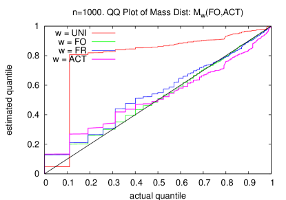
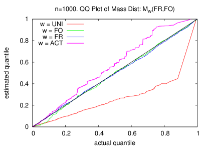
Figure 2: Quantile-Quantile Plot of Estimate vs. Actual Mass Distribution from 1000 Samples of Node Variables. fr and fo best estimated using either as sample weights.

Results for node variables are shown in Tables I and  II for ordinary and mass distributions, respectively. For ordinary distribution, the difference is noticeably smaller for uni and ac weightings than for fo and fr. This is unsurprising for uni; for ac it reflects the absence of strong correlations between large values of ac with other variables. For the mass distribution, we observe the difference for $D_{w}(X,X^{\prime})$ is typically smallest when $w=X$, regardless of the value of $X^{\prime}$. In other words, the mass distribution of $X$ relative to any other variable is generally most accurately estimated using $X$ as the sample weighting. However, the mass distributions of $X=\textsc{fo},\textsc{fr}$ have roughly equal estimation difference whichever is used as the weighting $w$. This reflects the fact that the distributions high values of fo and fr are fairly strongly correlated; see Section V. Table IV shows results for the mass distribution of the link variable ffan. The smallest estimation error using ffan weighting, although $\textsc{fo}_{2}$ weighting is reasonable, performing noticeably better than with uniform of $\textsc{fo}_{1}$ weighting.

We illustrate a selection of the estimated distributions through quantile-quantile plots of the estimated vs. actual mass distributions for a section of variables. Figure 2 shows the joint mass distributions of fo weighted by ac (left) and fr weighted by fo (right), where each line of the graph corresponds to a different sample weighing variable (uni, fo, fr, and ac). As expected, uni has the poorest performance, fo and fr the best (being highly correlated), while ac has variable performance. Figure 3 displays similar plots for the link fanout variable ffan, for both the self-weighted distribution (left) and the mass distribution with respect to the initial node follower count fo₁. In this case, estimation accuracy is, unsurprisingly, best for sample weighting with ffan itself. However, sampling weighting with fo₂, the numerator of ffan, also produces good results, while weighting with the denominator fo₁ is not so accurate. This is consistent with the observation that large values of ffan are driven more by large values in fo₂ than large values of fo₁.

w = uni	w = $\textsc{fo}_{1}$	w=$\textsc{fo}_{2}$	w=ffan
0.027	0.070	0.116	0.153

TABLE III: Ordinary Distribution Accuracy for Link Variable ffan: Median KS statistic for $D_{w}(\textsc{ffan})$ over 100 runs.

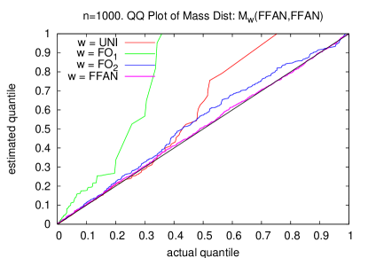
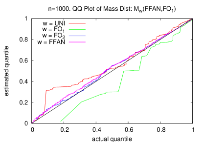
Figure 3: Quantile-Quantile Plot of Estimate vs. Actual Mass Distribution from 1000 Samples of Link Variable ffan. Best estimated using ffan as weight, $\textsc{fo}_{2}$ reasonable, uni and $\textsc{fo}_{1}$ poor.

w	X’ =$\textsc{fo}_{1}$	X’ = $\textsc{fo}_{2}$	X’=ffan
uni	0.231	0.279	0.300
$\textsc{fo}_{1}$	0.420	0.462	0.574
$\textsc{fo}_{2}$	0.065	0.061	0.064
ffan	0.034	0.027	0.025

TABLE IV: Mass Distribution Accuracy for Link Variables ffan: Median KS statistic for $D_{w}(\textsc{ffan},X^{\prime})$ over 100 runs.

VII Discussion and Conclusions

This paper was motivated by commercial interest in the joint distributional properties of users and the connections between them in online social networks. Although much research has been devoted to acquiring data through external crawling, OSN providers themelves are well positioned both to access OSN data directly through their customer databases and to monetize this as an information resource.

This paper proposes a method by which OSNs can provide samples of the user graph of tunable size, in non-intersecting increments, with sample selection that can be weighted to enhance accuracy when estimating different features of the graph. A key experimental conclusion what that neither uniform nor activity weighted sampling were accurate for estimating mass distributions of friends, followers and fanout, as compared with weighting by these features themselves.

To bring our approach to fruition requires two steps which we identify as future work. The first is to provide a method to systematically determine the set of required sample weightings as a function of the joint feature distribution and the class of queries to be served. The second is to provide an automated classification scheme that can dynamically select the best weighted sample set or sets to serve a given query.

References

- [1] Ahmed, N. K., Berchmans, F., Neville, J., and Kompella, R. Time-based sampling of social network activity graphs. In MLG ’10 (New York, NY, USA, 2010), ACM, pp. 1–9.
- [2] Alon, N., Duffield, N., Lund, C., and Thorup, M. Estimating arbitrary subset sums with few probes. In Proc. 24th ACM Symp. on Principles of Database Systems (PODS) (2005), pp. 317–325.
- [3] Becchetti, L. et. al.. A comparison of sampling techniques for web characterization. In Workshop on Link Analysis (LinkKDD) (August 2006).
- [4] Cha, M. et al.. Measuring user influence in twitter: The million follower fallacy. In ICWSM (2010).
- [5] Chaudhuri, S. et. al.. Overcomng limitations of sampling for aggregation queries. In ICDE’01 (2001), pp. 534–542.
- [6] Choudhury, M. et. al.. How does the sampling strategy impact the discovery of information diffusion in social media. In ICWSM (George Washington University, Washington, DC, May 2010).
- [7] Cohen, E., Duffield, N., Kaplan, H., Lund, C., and Thorup, M. Stream sampling for variance-optimal estimation of subset sums. In SODA ’09: Proceedings of the twentieth Annual ACM-SIAM Symposium on Discrete Algorithms (Philadelphia, PA, USA, 2009), Society for Industrial and Applied Mathematics, pp. 1255–1264.
- [8] Duffield, N., and Lund, C. Predicting resource usage and estimation accuracy in an ip flow measurement collection infrastructure. In ACM SIGCOMM Internet Measurement Workshop (2003). Miami Beach, Fl, October 27-29, 2003.
- [9] Duffield, N., Lund, C., and Thorup, M. Priority sampling for estimation of arbitrary subset sums. J. ACM 54, 6 (December, 2007), Article 32. Announced at SIGMETRICS’04.
- [10] Erdös, P., and Rényi, A. On Random Graphs. Publ. Math. Debrecen 6 (1959), 290–297.
- [11] Feldmann, A., Rexford, J., and Caceres, R. Efficient policies for carrying web traffic over flow-switched networks. IEEE/ACM Transactions on Networking (December 1998), 673–685.
- [12] Gjoka, M. et. al.. Walking in Facebook: A case study of unbiased sampling of OSNs. In INFOCOM (March 2010), IEEE, pp. 1–9.
- [13] Horvitz, D. G., and Thompson, D. J. A generalization of sampling without replacement from a finite universe. J. Amer. Stat. Assoc. 47, 260 (1952), 663–685.
- [14] Huberman, B., Romero, D., and Wu, F. Social networks that matter: Twitter under the microscope. In Social Science Research Network (December 2008).
- [15] Karkulahti, O., and Kangasharju, J. Youtube Revisited: On the Importance of Correct Measurement Methodology. Springer International Publishing, Cham, 2015, pp. 17–30.
- [16] Krishnamurthy, B., Gill, P., and Arlitt, M. A few chirps about Twitter. In WOSN (August 2008).
- [17] Kurant, M., Gjoka, M., Butts, C. T., and Markopoulou, A. Walking on a graph with a magnifying glass: stratified sampling via weighted random walks. In Proceedings of the ACM SIGMETRICS joint international conference on Measurement and modeling of computer systems (New York, NY, USA, 2011), SIGMETRICS ’11, ACM, pp. 281–292.
- [18] Kwak, H., Lee, C., Park, H., and Moon, S. What is twitter, a social network or a news media? In WWW (2010).
- [19] Leskovec, J., and Faloutsos, C. Sampling from large graphs. In KDD (New York, NY, USA, 2006), ACM, pp. 631–636.
- [20] Mislove, A., Marcon, M., Gummadi, K. P., Druschel, P., and Bhattacharjee, B. Measurement and analysis of online social networks. In Proceedings of the 7th ACM SIGCOMM Conference on Internet Measurement (New York, NY, USA, 2007), IMC ’07, ACM, pp. 29–42.
- [21] Ribeiro, B., and Towsley, D. Estimating and sampling graphs with multidimensional random walks. In IMC ’10 (New York, NY, USA, 2010), ACM, pp. 390–403.
- [22] Sachs, L. Applied Statistics. Springer, 1984.
- [23] Stutzbach, D., Rejaie, R., Duffield, N., Sen, S., and Willinger, W. On unbiased sampling for unstructured peer-to-peer networks. In Proceedings of the 6th ACM SIGCOMM Conference on Internet Measurement (New York, NY, USA, 2006), IMC ’06, ACM, pp. 27–40.
- [24] Sysomos. Insider twitter. http://www.sysomos.com/insidetwitter, July 2009.
- [25] Szegedy, M. The DLT priority sampling is essentially optimal. In Proc. 38th STOC (2006), pp. 150–158.
- [26] Twitter. The streaming API’s. https://dev.twitter.com/streaming/overview.
- [27] Wang, H., and Lu, J. Detect inflated follower numbers in osn using star sampling. In Proceedings of the 2013 IEEE/ACM International Conference on Advances in Social Networks Analysis and Mining (New York, NY, USA, 2013), ASONAM ’13, ACM, pp. 127–133.
- [28] Yabing Liu, C. K.-S., and Mislove, A. The tweets they are a-changin’: Evolution of Twitter users and behavior. In Proceedings of the 8th International AAAI Conference on Weblogs and Social Media (ICWSM’14) (Ann Arbor, MI, June 2014).
- [29] Zhang, Y., Kolaczyk, E. D., and Spencer, B. D. Estimating network degree distributions under sampling: An inverse problem, with applications to monitoring social media networks. Ann. Appl. Stat. 9, 1 (03 2015), 166–199.
- [30] Zhou, J., Li, Y., Adhikari, V. K., and Zhang, Z.-L. Counting youtube videos via random prefix sampling. In Proceedings of the 2011 ACM SIGCOMM Conference on Internet Measurement Conference (New York, NY, USA, 2011), IMC ’11, ACM, pp. 371–380.