Wormhole supported by dark energy admitting conformal motion

Abstract

In this article, we study the possibility of sustaining a static and spherically symmetric traversable wormhole geometries admitting conformal motion in Einstein gravity, which presents a more systematic approach to search a relation between matter and geometry. In wormhole physics, the presence of exotic matter is a fundamental ingredient and we show that this exotic source can be dark energy type which support the existence of wormhole spacetimes. In this work we model a wormhole supported by dark energy which admits conformal motion. We also discuss the possibility of detection of wormholes in the outer regions of galactic halos by means of gravitational lensing. The studies of the total gravitational energy for the exotic matter inside a static wormhole configuration are also done.

I Introduction

In last two decades, there has been a considerable interest in the field of wormhole physics after seminal work by Morris-Thorne Morris . They proposed the possibility of traversable wormholes in the theoretical context of the general relativity as a teaching tool. Topologically, wormholes acts as a tunnels in the geometry of space and time that connect two space-times of same universe or of different universes altogether by a minimal surface called the throat of the wormhole, satisfying flare-out condition HV1997 , through which a traveler can freely traverse in both directions. Today, most of the efforts are directed to study the necessary conditions to ensure their traversability. The most striking of these properties is a special type of matter that violates the energy conditions, called exotic matter which is necessary to construct traversable wormholes. Recent astronomical observations have confirmed that the universe is undergoing a phase of accelerated expansion which was conformed by the measurements of supernovae of type Ia (SNe Ia) and the cosmic microwave background anisotropy Riess . It has been suggested that dark energy is still an unknown component with a relativistic negative pressure, is a possible candidate for the present cosmic expansion and our Universe is composed of approximately 70 percent of it. The simplest candidate for explaining the dark energy is the cosmological constant $\Lambda$ Carmelli , which is usually interpreted physically as a vacuum energy, with $p=-\rho$. Another possible way to explain the dark energy by invoking an equation of state, p= $\omega\rho$ with $\omega<0$, where p is the spatially homogeneous pressure and $\rho$ the energy density of the dark energy, instead of the constant vacuum energy density. As a particular range of the $-1<$ $\omega<-1/3$, is a widely accepted results known as quintessence is often considered. The ratio $\omega<-1$ has been denoted phantom energy, corresponding to violation of the null energy condition, thus providing a theoretically supported scenario for the existence of wormholes Sushkov . The presence of phantom energy in the universe leads to peculiar properties, such as Big Rip scenario Caldwell , the black hole mass decreasing by phantom energy accretion Babichev . Therefore, the dark energy plays an important role in cosmology naturally makes us search for local astrophysical manifestation of it. In the present work we consider wormhole solution containing dark energy as equation of state.

The gravitational lensing (GL) is a very useful tool of probing a number of interesting phenomena of the universe. Particular it can provide rich information for the structure of compact astrophysical objects like e.g., black holes, exotic matter, super-dense neutron stars, wormholes etc. Out of this, the observation of Einstein ring and the double or multiple mirror images are the powerful examples for gravitational lensing effect Hewitt . In earlier works GL phenomenon has been studied in the weak field (see Schneider ), but success leads to explore other extreme regime, namely, the GL effect in the strong gravitational field has been studied by Virbhadra . Out of various intriguing objects mentioned above, recently it was proposed that wormholes can act as gravitational lenses and induce a microlensing signature on a background source studied by Kim and Sung Kim and Cramer et al., Cramer and lensing by negative mass wormholes have been studied by Safonova et al., Safonova . Related with the issue of GL effects on wormholes have been studied Nandi . Recently, the possibility of detection of traversable wormholes in noncommutative-geometry is studied by Kuhfittig Peter K. F. Kuhfittig in the outer regions of galactic halos by means of gravitational lensing. The possible existence of wormholes in the outer regions of the halo was discussed in Ref Rahaman(2014) , based on the NFW density profile. One of the aims of the current paper is to study the effect of lensing phenomenon for the wormhole solutions in the presence of exotic matter such as phantom fields admitting conformal motion. The present work has been considered in more systematic approach to find the exact solutions and study the natural relationship between geometry and matter. For instance, one may adopt a more systematic approach (see Ref. Herrera ) by assuming spherical symmetry and the existence of a non-static conformal symmetry. Suppose that a conformal Killing vector $\xi$ is defined on the metric tensor field g defined by the action of the Lie infinitesimal operator $\mathcal{L}_{\xi}$, which leads to the following relationship:

$$\mathcal{L}_{\xi}g_{ik}=\psi g_{ik},$$ (1)

where $\mathcal{L}$ is the Lie derivative operator and $\psi$ is the conformal factor. Here the vector $\xi$ generates the conformal symmetry in such a way that the metric g is conformally mapped onto itself along $\xi$. For an interesting observation neither $\xi$ nor $\psi$ need to be static even though one considers a static metric. For $\psi=0$ then Eq. (1) gives the killing vector, for $\psi=constant$ Eq. (1) gives a homothetic vector and if $\psi=\psi(x,t)$ then it gives conformal vectors. Further note that when $\psi=0$ the underlying spacetime is asymptotically flat which implies that the Weyl tensor will also vanish. Thus we can develop a more vivid idea about the spacetime geometry by studying the conformal killing vectors. Recently, Bohmer et al. Bohmer have studied the traversable wormholes under the assumption of spherical symmetry and the existence of a non-static conformal symmetry.

The outline of the present paper is as follows: In Sec. II. we give a brief outline of the conformal killing vectors for spherically symmetric metric while in Sec. III. we present the structural equation of phantom energy traversable wormholes and discuss the physical properties of our solution in the outer region of the halo by recalling the movement of a test particles. In Sec. IV. we present the stability of wormholes under the different forces where the total gravitational energy for the exotic matter distribution in the wormhole discuss in Sec. V. In Sec. VI. gravitational lensing has been studied and the angle of surplus are calculated. In Sec. VII. the interior wormhole geometry is matched with an exterior Schwarzschild solution at the junction interference. Finally, in Sec. VIII. we discuss some specific comments regarding the results obtained in the study.

II Einstein field equations and conformal killing vector

The spacetime metric representing a static and spherically symmetric line eleminent is given by

$$ds^{2}=-e^{\nu(r)}dt^{2}+e^{\lambda(r)}dr^{2}+r^{2}(d\theta^{2}+\sin^{2}\theta d\phi^{2}),$$ (2)

where $\lambda$ and $\nu$ are functions of the radial coordinate, r. We shall assume that our source is filled with an anisotropic fluid distribution and using the Einstein field equation $G_{\mu\nu}=8\pi T_{\mu\nu}$, for the above metric, which in our case read (with c = G = 1)

$$e^{-\lambda}\left[\frac{\lambda^{\prime}}{r}-\frac{1}{r^{2}}\right]+\frac{1}{r^{2}}=8\pi\rho,$$ (3)

$$e^{-\lambda}\left[\frac{1}{r^{2}}+\frac{\nu^{\prime}}{r}\right]-\frac{1}{r^{2}}=8\pi p_{r},$$ (4)

$$\frac{1}{2}e^{-\lambda}\left[\frac{1}{2}\nu^{\prime 2}+\nu^{\prime\prime}-\frac{1}{2}\lambda^{\prime}\nu^{\prime}+\frac{1}{r}(\nu^{\prime}-\lambda^{\prime})\right]=8\pi p_{t},$$ (5)

where $\rho$, $p_{r}$ and $p_{t}$ denotes the matter density, radial and transverse pressure respectively of the underlying fluid distribution. and ‘$\prime$’ denotes differentiation with respect to the radial coordinate r.

Applying a systematic approach in order to get exact solutions, we demand that the interior spacetime admits conformal motion (but neither $\xi$ nor $\psi$ need to be static even though for a static metric) and therefore Eq. (1) provides the following relationship:

$$\mathcal{L}_{\xi}g_{ik}=\xi_{i;k}+\xi_{k;i}=\psi g_{ik},$$ (6)

with $\xi_{i}=g_{ik}\xi^{k}$. The above equation gives the following set of expressions as

$$\xi^{1}\nu^{\prime}=\psi,~{}~{}~{}\xi^{4}=C_{1},~{}~{}~{}\xi^{1}=\frac{\psi r}{2}~{}~{}~{}and~{}~{}~{}\xi^{1}\lambda^{\prime}+2\xi^{1},_{1}=\psi,$$ (7)

where $C_{1}$ is a constant and the conformal factor is independent of time i.e., $\psi=\psi(r)$. Now, the metric (2), and using the Eq. (6-7) provides the following results:

$$e^{\nu}=C_{2}^{2}r^{2},$$ (8)

$$e^{\lambda}=\left(\frac{C_{3}}{\psi}\right)^{2},$$ (9)

$$\xi^{i}=C_{1}\delta_{4}^{i}+\left(\frac{\psi r}{2}\right)\delta_{1}^{i},$$ (10)

where $C_{2}$ and $C_{3}$ are constants of integrations.

An important note of this solutions that immediately ruled out, is that the conformal factor is zero by taking into account Eq. (9), at the throat of the wormhole i.e., $\psi(r_{0})=0$, where $r_{0}$ stands for location of the throat of the wormhole. Now, using Eqs. $(8)-(10)$, one can obtain the expression for Einstein field equations as

$$\frac{1}{r^{2}}\left[1-\frac{\psi^{2}}{C_{3}^{2}}\right]-\frac{2\psi\psi^{\prime}}{rC_{3}^{2}}=8\pi\rho,$$ (11)

$$\frac{1}{r^{2}}\left[\frac{3\psi^{2}}{C_{3}^{2}}-1\right]=8\pi p_{r},$$ (12)

$$\frac{\psi^{2}}{C_{3}^{2}r^{2}}+\frac{2\psi\psi^{\prime}}{rC_{3}^{2}}=8\pi p_{t}.$$ (13)

Observing the Eqs. $(11)-(13)$, we have three equations with four unknowns namely $\rho$, $p_{r}$, $p_{t}$ and $\psi(r)$ respectively. In order to solve the system of equations, we need an equation of state relating matter and density by the following simplest relation $p=p(\rho)$.

III Solution for phantom wormhole and physical analysis

According to Morris and Throne Morris , for constructing a wormhole solution one require an unusual form of matter known as ‘extotic matter’, which is the fundamental ingredient to sustain traversable wormhole. The characteristic of such matter is that the energy density $\rho$ may be positive or negative but the radial pressure $p_{r}$ must be negative. Theoretical advances shows that the expansion of our present universe is accelerating and dark energy is a suitable candidate to explain this cosmic expansion. In this context, we study the construction of traversable wormholes, using the phantom energy equation of state by the following relationship

$$p_{r}=\omega\rho~{}~{}~{}~{}~{}~{}~{}~{}~{}~{}with~{}~{}\omega<-1,$$ (14)

by taking into account Eqs. (11) and (12), with the help of equation (14) we obtain

$$\psi^{2}=\left(\frac{\omega+1}{\omega+3}\right)c_{3}^{2}+\psi_{0}r^{-\left(\frac{\omega+3}{\omega}\right)},$$ (15)

where $\psi_{0}$ is the constant of integration. For convenience we rewrite the Eqs. (11)-(13), using Eq. (15) with new dimensionless parameters $\tilde{\psi_{0}}$=$\frac{\psi_{0}}{c_{3}^{2}}$, we obtain the expression of matter density, radial and transverse pressure as

$$\rho = \frac{1}{8\pi}\left[\frac{2}{r^{2}\left(\omega+3\right)}-\tilde{\psi_{0}}\frac{\left(2\omega+3\right)}{\omega}r^{\frac{-3\left(\omega+1\right)}{\omega}}\right],$$ (16)

$$p_{r} = \frac{1}{8\pi}\left[\frac{2\omega}{r^{2}\left(\omega+3\right)}-\tilde{\psi_{0}}\left(2\omega+3\right)r^{\frac{-3\left(\omega+1\right)}{\omega}}\right],$$ (17)

$$p_{t} = \frac{1}{8\pi}\left[\frac{\omega+1}{r^{2}\left(\omega+3\right)}-\frac{3\tilde{\psi_{0}}}{\omega}r^{\frac{-3\left(\omega+1\right)}{\omega}}\right].$$ (18)

Plugging the expression for $\psi^{2}$ given in Eq. (9) with the dimensionless parameter the expression for metric potential is obtained as

$$e^{-\lambda}=\frac{\omega+1}{\omega+3}+\tilde{\psi_{0}}r^{-\left(\frac{\omega+3}{\omega}\right)}.$$ (19)

Thus, taking into account the relation between metric potential and the shape function of the wormhole by the relation $e^{\lambda}=\frac{1}{1-b(r)/r}$, we obtain form of shape function as

$$b(r)=\frac{2r}{\omega+3}-\tilde{\psi_{0}}r^{-\frac{3}{\omega}}.$$ (20)

From the expression of $b(r)$, we see that $\frac{b(r)}{r}$ tends to a finite value as $r\rightarrow\infty$ and the redshift function does not approach zero as $r\rightarrow\infty$, so spacetime is not asymptotically flat due to the conformal symmetry.

Now, we will concentrate to verify whether the obtained expression for the shape function $b(r)$ satisfies all the physical requirements to maintain a wormhole solution. For this purpose we are trying to describe fundamental property of wormholes with help of graphical representation. The profile of shape function $b(r)$ is plotted in Fig. 1 for the values of $\tilde{\psi_{0}}=0.09$ and $\omega=-1.58$, where the flaring out condition has been checked in Fig. 1 (right panel). We observe that shape function is decreasing with increase of the radius, and $\frac{db(r)}{dr}<0$ for $r>10.45$. From the left panel of Fig. 2, we observe that the throat of the wormhole occurs where $b(r)-r$ cuts the r axis at a distance $r=5.39$. Therefore the throat of the wormhole occurs at $r=5.39$ Km. for our present model. Consequently, we observe that $b^{\prime}(5.39)=0.632<1$ and for $r>r_{0}$ we see that $b(r)-r<0$, which implies $\frac{b(r)}{r}<1$ for $r>r_{0}$, strongly indicate that our solution satisfy all the physical criteria for wormhole solution. The slope of $b(r)$ is positive upto $r=10.45$, which concludes that the wormhole can not be arbitrarily large. The same situation occurred in the previous work bhar . Moreover, we consider the energy conditions and the violation of the null energy condition (NEC) i.e., $\rho+p_{r}<~{}0$, is a necessary property for a static wormhole to exist. In Fig. 2 (right panel), we have studied all types of energy condition (using Eqs.(16)-(18)), graphically and observed that our solution violated the NEC to hold a wormhole open.

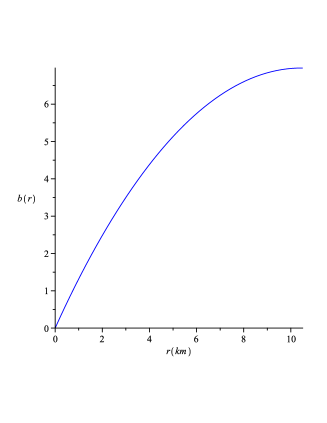
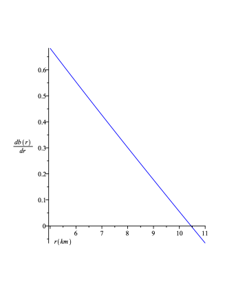
Figure 1: The shape function b(r) is plotted against r left panel. The values of the parameters are $\tilde{\psi_{0}}=0.09$ and $\omega=-1.58$. The slope of shape function of wormhole is plotted in the right panel with the same parametric values. The figure indicates that the slope of $b(r)$ is still positive within the range of r = 10.45.

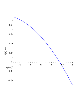
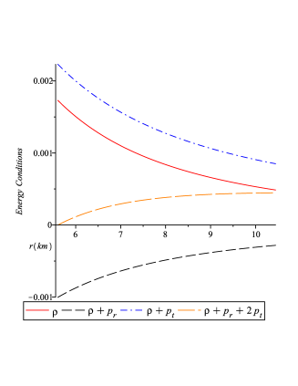
Figure 2: The profile of $b(r)-r$ is plotted against r in the left panel with the same values of parameters as stated earlier. The throat of the wormhole occurs where the graph of $b(r)-r$ cuts the r axis and for our model the throat occurs at r=5.39 Km. The energy conditions are plotted in the right panel. The figure indicates the null energy condition is violated for wormhole model.

Since, the wormhole space-time is non-asymptotically flat and hence the wormhole spacetime should match at some junction radius $r=R$, to the exterior schwarzschild spacetime given by the following metric

$$ds^{2} = -\left(1-\frac{2M}{r}\right)dt^{2}+\left(1-\frac{2M}{r}\right)^{-1}dr^{2}$$ (21)

$$+r^{2}\left(d\theta^{2}+\sin^{2}\theta d\phi^{2}\right).$$

Here the matching occurs at a radius greater than the event horizon which gives

$$\left(\frac{R}{b_{0}}\right)^{2}=1-\frac{2M}{R}~{}~{}~{}and~{}~{}~{}1-\frac{b(R)}{R}=1-\frac{2M}{R},$$ (22)

and using the Eq. (8) with the expression $e^{\nu(R)}=c_{2}^{2}R^{2}$, we determine the values of the constants $c_{2}^{2}$, $b_{0}$ and total mass M as follows

$$M = \frac{R}{\omega+3}-\frac{\tilde{\psi_{0}}}{2}R^{-\frac{3}{\omega}},$$ (23)

$$c_{2}^{2} = \frac{1}{R^{2}}\left[\frac{\omega+1}{\omega+3}+\tilde{\psi_{0}}R^{-\frac{3+\omega}{\omega}}\right],$$ (24)

$$b_{0} = \frac{R}{\frac{\omega+1}{\omega+3}+\tilde{\psi_{0}}R^{-\frac{3+\omega}{\omega}}}.$$ (25)

IV TOV Equation

An important step is to examine the stability of our present model under the different forces namely gravitational, hydrostatics and anisotropic forces. This is simply by considering the generalized Tolman-Oppenheimer-Volkov (TOV) equation according to Ponce de Le$\acute{o}$n leon

$$-\frac{M_{G}(r)(\rho+p_{r})}{r}e^{\frac{\nu-\mu}{2}}-\frac{dp_{r}}{dr}+\frac{2}{r}(p_{t}-p_{r})=0,$$ (26)

where $M_{G}(r)$ represents the effective gravitational mass within the radius $r$, which can derived from the Tolman-Whittaker formula and the explicit expression is given by

$$M_{G}(r)=\frac{1}{2}re^{\frac{\mu-\nu}{2}\nu^{\prime}}.$$ (27)

Substituting the above expression in Eq. (26), we obtain the simple expression as

$$-\frac{\nu^{\prime}}{2}(\rho+p_{r})-\frac{dp_{r}}{dr}+\frac{2}{r}(p_{t}-p_{r})=0.$$ (28)

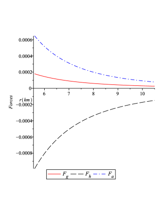
Figure 3: Variation of different forces acting on the wormhole are plotted against r with the same values of parameters as stated earlier in Fig. 1.

Therefore, one can write it in a more suitable form to generate the simpler equation

$$F_{g}+F_{h}+F_{a}=0,$$ (29)

where $F_{g}=-\frac{\nu^{\prime}}{2}(\rho+p_{r})$, $F_{h}=-\frac{dp_{r}}{dr}$ and $F_{a}=\frac{2}{r}(p_{t}-p_{r})$ represents the gravitational, hydrostatics and anisotropic forces, respectively. Using the Eqs. (16-18), the above expression can be written as

$$F_{g}=-\frac{(\omega+1)}{8\pi r}\left[\frac{2}{r^{2}\left(\omega+3\right)}-\frac{\tilde{\psi_{0}}\left(2\omega+3\right)}{\omega}r^{-\frac{3\left(\omega+1\right)}{\omega}}\right],$$ (30)

$$F_{h}=\frac{1}{8\pi}\left[\frac{4\omega}{r^{3}\left(\omega+3\right)}-\frac{3\tilde{\psi_{0}}\left(2\omega+3\right)\left(\omega+1\right)}{\omega}r^{-\frac{\left(4\omega+3\right)}{\omega}}\right],$$ (31)

$$F_{a}=\frac{1}{4\pi r}\left[\frac{1-\omega}{r^{2}\left(\omega+3\right)}+\frac{\tilde{\psi_{0}}\left(2\omega^{2}+3\omega-3\right)}{3}r^{-\frac{3\left(\omega+1\right)}{\omega}}\right].$$ (32)

The profiles of $F_{g},F_{h},$ and $F_{a}$ for our present model of wormhole are shown in Fig. $3$, by assigning the same value of $\omega$ = -1.58 and $\tilde{\psi_{0}}=0.09$ as we used in Fig. $1$. It is clear from the Fig. 3, that the hydrostatics force ($F_{h}$) is dominating compare to gravitational ($F_{g}$) and anisotropic forces ($F_{a}$), respectively. The interesting feature is that $F_{h}$ takes the negative value while $F_{g}$ and $F_{a}$ are positive, which clearly indicate that hydrostatics force is counterbalanced by the combine effect of gravitational and anisotropic forces to hold the system in static equilibrium. There exist many excellent reviews on this topic have been studied in-depth by Rahaman et al. rah16 and Rani & Jawad jawad .

The obtained values of $E_{g}$
r	$E_{g}$
6	2.777766660
6.5	2.711356872
7	2.618496680
7.5	2.506836836
8	2.380794614
8.5	2.243339402
9	2.096641966
9.5	1.942376899
10	1.781885447
10.45	1.633036240

Table 1: The values of $E_{g}$ are obtained from the Eq. (37), for the choices of the parameters $r_{0}^{+}=5.6$ km, $\tilde{\psi_{0}}=0.09$ and $\omega=-1.58$.

V Active mass function and Total Gravitational Energy

The active mass function for our wormhole ranging from $r_{0}+$ ($r_{0}$ is the throat of the wormhole) up to the radius R can be found as

$$M_{active}=\int_{r_{0}+}^{R}4\pi\rho r^{2}dr=\left[\frac{r}{\omega+3}+\frac{\tilde{\psi_{0}}\left(2\omega+3\right)}{6}r^{\frac{-3}{\omega}}\right]_{r_{0}+}^{R}.$$ (33)

The active gravitational mass function of the wormhole is plotted in of Fig. 4 (left panel). From the Fig. 4, we see that $M_{\mathrm{active}}$ is positive outside the wormhole throat and monotonic increasing function of the radial co-ordinate, r.

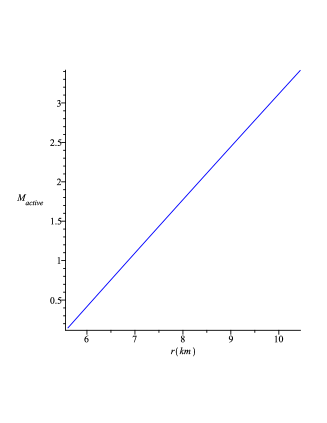
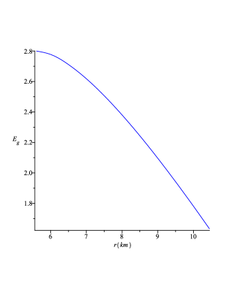
Figure 4: Active gravitational mass of the wormhole is plotted against r in the left panel and Total gravitational energy is plotted against r in the right panel by taking the same values of the model parameters.

For the study of total gravitational energy of the exotic matter inside a static wormhole configuration we use the procedure adopted by Lyndell-Bell et al. and Nandi et al. lyn ; Amrita ; nandi for calculating the total gravitational energy $E_{g}$ of the wormhole, can be written in the form

$$E_{g}=Mc^{2}-E_{M},$$ (34)

where the total mass-energy within the region from the throat $r_{0}$ up to the radius R can be provided as

$$Mc^{2}=\frac{1}{2}\int_{r_{0}^{+}}^{R}T_{0}^{0}r^{2}dr+\frac{r_{0}}{2},$$ (35)

and the energy in other forms like kinetic energy, rest energy, internal energy etc. are defined by

$$E_{M}=\frac{1}{2}\int_{r_{0}^{+}}^{R}\sqrt{g_{rr}}\rho r^{2}dr.$$ (36)

Note that here $\frac{4\pi}{8\pi}$ yields the factor $\frac{1}{2}$. By taking into account Eqs. (34 - 36), we obtain

$$E_{g}=\frac{1}{2}\int_{r_{0}^{+}}^{R}[1-(g_{rr})^{\frac{1}{2}}]\rho r^{2}dr+\frac{r_{0}}{2},$$ (37)

where $g_{rr}=\left(1-\frac{b(r)}{r}\right)^{-1}$ and $r_{0}$ is the throat of the wormhole. Now to find out the expression of total gravitational energy $E_{g}$, we have performed the integral of Eq. (37). Due to the complexity of the coefficients $g_{rr}$ and $\rho$ we cannot extract analytical solution, for that we solve the integral numerically. The numerical values of $E_{g}$ are obtained by taking $r_{0}^{+}=5.6$ Km. as a lower limit and by changing the upper limits, which are given in Table. I.

VI Gravitational Lensing

We know that a photon follows a null geodesic $ds^{2}=0$, when external forces are absent. Then the equation of motion of a photon can be written as :

$$\dot{r}^{2}+e^{-\lambda}r^{2}\dot{\phi}^{2}=e^{\nu-\lambda}c^{2}\dot{t}^{2},$$ (38)

where the dot represents derivative with respect to the arbitrary affine parameter. Since, neither $t$ nor $\phi$ appear explicitly in the variation principle, their conjugate momenta yield the following constants of motion :

$$e^{\nu}c^{2}\dot{t}=E=\text{constant},$$ (39)

$$r^{2}\dot{\phi}=L=\text{constant},$$ (40)

where $E$ and $L$ are related with the conservation of energy and angular momentum, respectively. Using these two constants of motion in Eq. (38), we get

$$\dot{r}^{2}+e^{-\lambda}\frac{L^{2}}{r^{2}}=\frac{E^{2}}{c^{2}}e^{-\nu-\lambda}.$$ (41)

Now, using $r=\frac{1}{u}$ and eliminating the derivatives with respect to the affine parameter by the help of the conservation equations, we obtain

$$\left(\frac{du}{d\phi}\right)^{2}+u^{2}=f(u).u^{2}+\frac{1}{c^{2}}\frac{E^{2}}{L^{2}}e^{-\nu-\lambda}\equiv P(u),$$ (42)

where $e^{-\lambda}=1-f(u)$, while from Eq. (19) yields

$$f(u)=\frac{2}{\omega+3}-\tilde{\psi}_{0}u^{\frac{\omega+3}{\omega}}.$$ (43)

Moreover, from Eq. (42), we get

$$P(u)=\frac{u^{2}}{\omega+3}\left(2+\frac{E^{2}b_{0}^{2}(\omega+1)}{c^{2}L^{2}}\right)+\tilde{\psi}_{0}u^{\frac{3(\omega+1)}{\omega}}\left(\frac{E^{2}b_{0}^{2}}{c^{2}L^{2}}-1\right).$$ (44)

Let us proceed to discuss at the turning points lake , the derivative of the radial vector with respect to the affine parameter vanishes, which in turn leads to $\frac{du}{d\phi}=0$. Consequently the turning point is denoted by $r_{\Sigma}=1/u_{\Sigma}$ and given by

$$r_{\Sigma}=\left(-\tilde{\psi_{0}}\frac{\omega+3}{\omega+1}\right)^{\frac{\omega}{\omega+3}}.$$ (45)

The deflection angles $\delta$ are listed for different values of w
$\omega$	$\phi$	$\delta$
-1.38	1.126922	-.887746
-1.4	1.1130334357	-.915523128
-1.58	1.0061484	-1.1292932
-1.8	0.903820943	-1.333948114
-2.1	0.7825234	-1.5765432
-2.3	0.696393	-1.748804
-2.4	0.98541384	-1.17076232
-2.7	0.406932726	-2.327724548

Table 2: The values of $\delta$ are obtained for the different choices of the parameters $\omega$ when $\tilde{\psi_{0}}=0.09$.

Differentiating Eq. (42) with respect to $\phi$, we get

$$\frac{d^{2}u}{d\phi^{2}}+u=Q(u),$$ (46)

where $Q(u)=\frac{1}{2}\frac{dP(u)}{du}$, and define by

$$Q(u) = \frac{u}{\omega+3}\left(2+\frac{E^{2}b_{0}^{2}(\omega+1)}{c^{2}L^{2}}\right)$$ (47)

$$+\frac{3\tilde{\psi}_{0}(\omega+1)}{2\omega}u^{\frac{2\omega+3}{\omega}}\left(\frac{E^{2}b_{0}^{2}}{c^{2}L^{2}}-1\right).$$

Now, if the deflective source are absent, then the equation (46) modified to

$$u=\frac{cos(\phi)}{R},$$ (48)

which is a straight line with R is the distance of closest approach to the wormhole. This solution can treated as first approximation. Furthermore, we use this solution as the first approximation to get the general solution. This yields the following form of Eq. (47) as

$$\frac{d^{2}u}{d\phi^{2}}+u=A\cos\phi+B(\cos\phi)^{\frac{2\omega+3}{\omega}},$$ (49)

where

$$A=\frac{2}{R(\omega+3)}+\frac{E^{2}b_{0}^{2}(\omega+1)}{Rc^{2}L^{2}(\omega+3)},\mathrm{and}~{}~{}B=\frac{3\tilde{\psi}_{0}(\omega+1)}{2\omega}\left(\frac{E^{2}b_{0}^{2}}{c^{2}L^{2}}-1\right).$$

With the aid of Eq. (49), the general solution is given by

$$u = \frac{\cos\phi}{R}+\frac{A}{2}\left(\cos\phi+\phi\sin\phi\right)+$$

$$B\sin\phi\int\cos^{\frac{3(\omega+1)}{\omega}}\phi~{}~{}d\phi+B\frac{\omega}{3(\omega+1)}\cos^{\frac{4\omega+3}{\omega}}\phi.$$

. (50)

The light ray approaches from infinity at an asymptotic angle $\phi=-\left(\frac{\pi}{2}+\epsilon\right)$ and goes back to infinity at an asymptotic angle $\phi=\left(\frac{\pi}{2}+\epsilon\right)$. However the point of transition of the light ray from the Schwarzschild spacetime to the phantom spacetime is given by the turning points defined in (45). The solution of the equation $~{}~{}u\left(\frac{\pi}{2}+\epsilon\right)=0$ yields the angle $\epsilon$. The total deflection angle of the light ray can be obtained as $\delta=2\epsilon$. In case of our wormhole, we have calculated the deflection angles for different values of $\omega$ that are tabulated in Table II. One can note that rather finding angle of deficit, we have found angle of surplus.

Lastly we must remember that the phantom spacetime under consideration, unlike Schwarzschild, is basically non flat. Hence strictly speaking, an asympotically straight line trajectory where $r\rightarrow\infty$ does not make sense. To resolve this issue we can consider the angles which the tangent to the light trajectory makes with the coordinate planes at a given point. Following Rindler and Ishak Rindler we can find

$$\tan(\Psi)=\frac{r\left[e^{\nu(r)}\right]^{1/2}}{\left|\frac{dr}{d\phi}\right|}~{},$$ (51)

using Eq. [42] we have

$$\tan(\Psi)=\sqrt{\frac{\frac{1}{R^{2}}\left[\frac{\omega+1}{\omega+3}+\tilde{\psi}_{0}R^{-(3+\omega)/\omega}\right]}{\frac{AR-1}{r^{2}}+\frac{2B\omega}{3(\omega+1)}r^{-3(\omega+1)/\omega}}}.$$ (52)

Assuming the bending angle to be small we can take $\tan(\Psi)\rightarrow\Psi$, $\sin(\phi)\rightarrow\phi$ and $\cos(\phi)\rightarrow 1$. Thus from Eq. [VI] we can write the actual light deflection angle given by $|\epsilon|=\left|\Psi-\phi\right|$ as follows :

$$|\epsilon|=\left|\sqrt{\frac{\frac{1}{R^{2}}\left[\frac{\omega+1}{\omega+3}+\tilde{\psi}_{0}R^{-(3+\omega)/\omega}\right]}{\frac{AR-1}{r^{2}}+\frac{2B\omega}{3(\omega+1)}r^{-3(\omega+1)/\omega}}}-\left[\frac{\frac{1}{r}-\frac{1}{R}-\frac{A}{2}-\frac{B\omega}{3(\omega+1)}}{B+\frac{A}{2}}\right]\right|.$$ (53)

Working along the lines of Bhadra et. al. Bhadra we can then calculate the total deflection angle in terms of location of the source ($d_{LS},\phi_{S}$) and the observer ($d_{OL},\phi_{O}$) as

$$|\epsilon| = \left|\sqrt{\frac{\frac{1}{R^{2}}\left[\frac{\omega+1}{\omega+3}+\tilde{\psi}_{0}R^{-(3+\omega)/\omega}\right]}{(AR-1)\left(\frac{1}{d_{LS}^{2}}+\frac{1}{d_{OL}^{2}}\right)+\frac{2B\omega}{3(\omega+1)}\left(d_{LS}^{-3(\omega+1)/\omega}+d_{OL}^{-3(\omega+1)/\omega}\right)}}\right.$$

$$\left.-\left[\frac{\frac{1}{d_{LS}}+\frac{1}{d_{OL}}-\frac{1}{R}-\frac{A}{2}-\frac{B\omega}{3(\omega+1)}}{B+\frac{A}{2}}\right]~{}\right|.$$

VII Junction Condition

In previous section we matched our interior wormhole spacetime with the Schwarzschild exterior spacetime at the boundary $r=r_{\Sigma}$. Since the wormhole spacetime is not asymptotically flat we use the Darmois Israel dm1 ; dm2 formation to determine the surface stresses at the junction boundary. The intrinsic surface stress energy tensor $S_{ij}$ is given by Lancozs equations in the following form

$$S^{i}_{j}=-\frac{1}{8\pi}(\kappa^{i}_{j}-\delta^{i}_{j}\kappa^{k}_{k}).$$ (55)

The second fundamental form is presented by

$$K_{ij}^{\pm}=-n_{\nu}^{\pm}\left[\frac{\partial^{2}X_{\nu}}{\partial\xi^{i}\partial\xi^{j}}+\Gamma_{\alpha\beta}^{\nu}\frac{\partial X^{\alpha}}{\partial\xi^{i}}\frac{\partial X^{\beta}}{\partial\xi^{j}}\right]|_{S},$$ (56)

and the discontinuity in the second fundamental form is written as,

$$\kappa_{ij}=K_{ij}^{+}-K_{ij}^{-},$$ (57)

where $n_{\nu}^{\pm}$ are the unit normal vectors defined by,

$$n_{\nu}^{\pm}=\pm\left|g^{\alpha\beta}\frac{\partial f}{\partial X^{\alpha}}\frac{\partial f}{\partial X^{\beta}}\right|^{-\frac{1}{2}}\frac{\partial f}{\partial X^{\nu}},$$ (58)

with $n^{\nu}n_{\nu}=1$. Where $\xi^{i}$ is the intrinsic coordinate on the shell. $+$ and $-$ corresponds to exterior i.e., Schwarzschild spacetime and interior (our) spacetime respectively.

Considering the spherical symmetry of the spacetime surface stress energy tensor can be written as $S^{i}_{j}=diag(-\sigma,\mathcal{P})$. Where $\sigma$ and $\mathcal{P}$ is the surface energy density and surface pressure respectively. The expression for surface energy density $\sigma$ and the surface pressure $\mathcal{P}$ at the junction surface $r=r_{\Sigma}$ are obtained as,

$$\sigma = -\frac{1}{4\pi r_{\Sigma}}\left[\sqrt{e^{-\lambda}}\right]_{-}^{+}$$ (59)

$$=-\frac{1}{4\pi r_{\Sigma}}\left[\sqrt{1-\frac{2M}{r_{\Sigma}}}-\sqrt{\frac{\omega+1}{\omega+3}+\tilde{\psi_{0}}r_{\Sigma}^{-\frac{3+\omega}{\omega}}}\right],$$

and

$$\mathcal{P} = \frac{1}{8\pi r_{\Sigma}}\left[\left\{1+\frac{a\nu^{\prime}}{2}\right\}\sqrt{e^{-\lambda}}\right]_{-}^{+}$$ (60)

$$=\frac{1}{8\pi r_{\Sigma}}\left[\frac{1-\frac{M}{r_{\Sigma}}}{\sqrt{1-\frac{2M}{r_{\Sigma}}}}-\sqrt{\frac{\omega+1}{\omega+3}+\tilde{\psi_{0}}r_{\Sigma}^{-\frac{3+\omega}{\omega}}}\right].$$

Hence we have matched our interior Wormhole solution to the exterior Schwarzschild spacetime in presence of thin shell.

VIII Discussion

By the confirmation of various observational data that the Universe is undergoing a phase of accelerated expansion and dark energy models have been proposed for this expansion. In the framework of GR, the violation of NEC namely ‘exotic matter’, is a fundamental ingredient of static traversable wormholes. In this work, we investigated some of the characteristics needed to support a traversable wormhole specific exotic form of dark energy, denoted phantom energy, admitting conformal motion of Killing Vectors. We analyzed the physical properties and characteristics of these wormholes with help of graphical representation. In the plots of Fig. 2 (left panel). we obtain the throat of wormholes where $b(r)-r$ cuts the r-axis, is located at r = $r_{0}$ = 5.39 Km., which implies that $b(r)/r<1$, met the flare-out condition. Another fundamental property of wormhole is the violation of the null energy condition (NEC), also satisfy for our model given in Fig. 2 (right panel), which provide a natural scenario for the existence of traversable wormholes. We discuss the possibility of detection of wormholes by means of gravitational lensing and we have found the angle of deflection to be negative i.e. angle of surplus. Additionally in order to give a physically feasible meaning to light deflection in a nonflat phantom spacetime, we have computed the angles that the tangent to the light trajectory makes with the coordinate planes in terms of the location of the observer and the source. Further we investigate, total gravitational energy content in the interior of exotic matter distribution for the wormholes by Lyndell-Bell et al. lyn and Nandi et al’s.nandi perception. This lensing phenomena i.e. deflection of light by the wormhole offers a good possibility to detect the presence of wormhole. The present study offers a clue for possible detection of wormholes and may encourage researchers to seek observational evidence for wormholes.

Acknowledgments

AB and FR would like to thank the authorities of the Inter-University Centre for Astronomy and Astrophysics, Pune, India for providing research facilities. FR is also grateful to DST-SERB and DST-PURSE, Govt. of India for financial support. We are also thankful to the referee for his constructive suggestions.

References

- (1) M. Morris and K. Thorne :Am. J. Phys., 56, 395 (1988).
- (2) D. Hochberg and M. Visser :Phys.Rev.D, 56, 4745 (1997).
- (3) A. G. Riess et al., :Astronomical Journal , 116, 1009 (1998); S. Perlmutter et al., : Astrophys. J. , 517, 565 (1999); C. L. Bennett et al., : Astrophys. J. Suppl. Ser., 148, 1 (2003).
- (4) M. Carmelli : [arXiv:astro-ph/ 0111259].
- (5) S. V. Sushkov : Phys. Rev. D, 71, 043520 (2005); O. B. Zaslavskii : Phys. Rev. D, 72, 061303 (2005); P. K. F. Kuhfittig : Class. Quant. Grav., 23, 5853-5860 (2006); F. S. N. Lobo : Phys. Rev. D, 71, 084011 (2005); F. Rahaman et al., :Phys. Lett. B , 633, 161-163 (2006); M Jamil, et al., :Eur. Phys. J. C , 67, 513-520 (2010).
- (6) R. R. Caldwell et al.,: Phys. Rev. Lett., 91, 071301(2003).
- (7) E. Babichev et al., : Phys. Rev. Lett. , 93, 021102 (2004).
- (8) J. N. Hewitt et al., : Nature (London), 333, 537 (1988); J. Wambsganss : Gravitational Lensing in Astronomy - astro-ph/ 9812021.
- (9) P. Schneider, J. Ehlers, and E. E. Falc : Gravitational Lenses (Springer-Verlag, Berlin, 1992).
- (10) K. S. Virbhadra and C. R. Keeton : Phys. Rev. D , 77, 124014 (2008); K. S. Virbhadra :Phys. Rev. D, 79, 083004 (2009); V. Bozza :Gen. Relativ. Gravit., 42, 2269 (2010); V. Bozza and L. Mancini : ApJ., 753, 56 (2012).
- (11) S. W. Kim and Y. M. Cho : Evolution of the Universe and its Observational Quest (Universal Academy Press, Inc. and Yamada Science Foundation, 1994), p. 353.
- (12) J. G. Cramer et al., : Phys. Rev. D 51, 3117 (1995).
- (13) M. Safonova et al., : Phys. Rev. D , 65, 023001 (2002).
- (14) K. K. Nandi et al., : Phys. Rev. D, 74 , 024020 (2006); M. Safonova et al., : Mod. Phys. Lett. A, 16, 153 (2001); E. Eiroa et al., : Mod. Phys. Lett. A, 16, 973 (2001); M. Safonova et al., : Phys. Rev. D, 65, 023001 (2001); M. Safonova and D. F. Torres : Mod. Phys. Lett. A, 17, 1685 (2002); F. Rahaman et al., : Chin. J. Phys., 45, 518 (2007).
- (15) P. K. F. Kuhfittig : arXiv - 1501.06085 [gr-qc].
- (16) F. Rahaman et al., : Eur. Phys. J. C, 2750, 74 (2014).
- (17) L. Herrera et al., : J. Math. Phys., 25, 3274 (1984); L. Herrera et al., : J. Math. Phys. , 26, 2302 (1985); R. Maartens and M. S. Maharaj : J. Math. Phys., 31, 151 (1990).
- (18) C. G. Böhmer, T. Harko, F. S. N. Lobo : Class.Quant.Grav., 27, 185013 (2010).
- (19) P. Bhar and F. Rahaman : Eur. Phys. J. C, 74, 3213 (2014).
- (20) J. Ponce de León : Gen. Relativ. Gravit., 25, 1123 (1993).
- (21) D. Lynden-Bell, J. Katz, J. Bik : Phys. Rev. D, 75, 024040 (2007).
- (22) A. Bhattacharya et al., : Class. Quant. Grav., 26, 235017 (2009).
- (23) K. K. Nandi et al., : Phys. Rev. D , 79, 024011 (2009).
- (24) K. Lake : Phys. Rev. D, 65, 087301 (2002).
- (25) W. Rindler and M. Ishak Phys. Rev. D, 76, 043006 (2007).
- (26) A. Bhadra et al., : Phys.Rev.D, 82, 063003 (2010).
- (27) W. Israel : Nuo. Cim. B, 44, 1 (1966); erratum - ibid. 48, 463 (1967); F. Rahaman et al., : Gen. Relativ. Gravit., 38, 1687 (2006);
- (28) F. Rahaman et al., : Physics Letters B, 746, 73 (2015).
- (29) S. Rani and A. Jawad : arxiv - 1603.08503 v2
- (30) W. Israel, Nuovo Cimento B 44, 1 (1966)
- (31) W. Israel, Nuovo Cimento B 48, 463 (1967). (Erratum)