Abstract

We discuss weak kaon decays in a scenario in which the Standard Model is extended by massive sterile fermions. After revisiting the analytical expressions for leptonic and semileptonic decays we derive the expressions for decay rates with two neutrinos in the final state. By using a simple effective model with only one sterile neutrino, compatible with all current experimental bounds and general theoretical constraints, we conduct a thorough numerical analysis which reveals that the impact of the presence of massive sterile neutrinos on kaon weak decays is very small, less than $1\%$ on decay rates. The only exception is ${\mathcal{B}}(K_{L}\to\nu\nu)$, which can go up to $\mathcal{O}(10^{-10})$, thus possibly within the reach of the KOTO, NA62 and SHIP experiments. Plans have also been proposed to search for this decay at the NA64 experiment. In other words, if all the future measurements of weak kaon decays turn out to be compatible with the Standard Model predictions, this will not rule out the existence of massive light sterile neutrinos with non-negligible active-sterile mixing. Instead, for a sterile neutrino of mass below $m_{K}$, one might obtain a huge enhancement of ${\mathcal{B}}(K_{L}\to\nu\nu)$, otherwise negligibly small in the Standard Model.

1 Introduction

The Standard Model (SM) predicts the strict conservation of lepton flavor to all orders. The fact that neutrinos oscillate provides clear evidence of the existence of physics beyond the Standard Model. New physics models accommodating massive neutrinos and their mixing open the door to many phenomena which basically have no Standard Model background, such as lepton number violation, violation of lepton flavor universality, or lepton flavor violation.

The experimental effort associated with the search of new physics using observables involving leptons is impressive, and is currently being pursued on all experimental fronts: (i) neutrino dedicated experiments which aim to determine neutrino properties, such as the Majorana/Dirac nature, the absolute neutrino masses, the hierarchy of their mass spectrum, leptonic mixing and the CP-violating phases; (ii) high-intensity facilities that are studying several low-energy processes such as $\ell\to\ell^{\prime}\gamma$, $\ell_{k}\to\ell_{i}\ell_{i}\ell_{j}$, $\mu-e$ conversion in atoms, $\tau$ and meson $M$ decays ($\tau\to M\nu$, $M\to\ell\nu$, $M\to M^{\prime}\ell\nu$, $M\to M^{\prime}\ell\ell,M^{\prime}\nu\nu$, …); (iii) the Large Hadron Collider (LHC), which is the privileged discovery ground of new particles, may also allow one to probe leptonic mixing in the production and/or decay of the new states. On the other hand, the recent cosmological data have put constraints on the sum of the light neutrino masses, which is especially restrictive when considering new light neutral states.

Among the several minimal possible scenarios, extending the SM with sterile fermions – which are singlets under the Standard Model gauge group – is a very appealing hypothesis, as their unique (indirect) interaction with the Standard Model fields occurs through their mixing with the active neutrinos $\nu_{L}$ (via their Yukawa couplings). Due to their very unique nature, there is no bound on their number, and a priori no limits regarding their mass regimes. Interestingly, sterile fermions (like right-handed neutrinos) are present in many frameworks accounting for neutrino masses and the observed mixing (as is the case for fermion seesaw mechanisms). The interest in sterile neutrinos and their impact on observables strongly depend on their masses. Sterile neutrinos at the eV scales were proposed to solve neutrino oscillation anomalies in reactors [1], accelerators [2], as well as in the calibration of gallium-target solar neutrino experiments [3], all suggesting beyond the three-neutrino paradigm. The keV scale for sterile neutrinos offers warm dark matter candidates [4, 5], and explanations of some astrophysical issues such as kicks in pulsar velocities [6]. Sterile fermion states with masses above $10^{9}$ GeV have moderate motivation other than their theoretical appeal (grand unified theories) and the possibility to have a scenario for baryogenesis via the high-scale leptogenesis [7]. Finally, the appeal for sterile neutrinos in the range ${\rm MeV}-{\rm GeV}$ (and even TeV) strongly resides in their experimental testability due to the many direct and indirect effects in both high-energy (e.g. LHC) [8] and high-intensity (e.g., NA62, NA64) experiments.

In order to illustrate the phenomenological effect of a scenario which involves sterile fermions, we focus on a minimal model which extends the Standard Model with an arbitrary number of sterile states with masses in the above-mentioned ranges, known as $3+N$ models, without making assumptions concerning the neutrino mass (and/or the lepton mixing) generation mechanism, but allowing one to access the degrees of freedom of the sterile neutrinos (their masses, their mixing with the active neutrinos and the new CP-violating phases). In this work, we address the phenomenological imprints of such sterile fermions on observables involving kaon meson rare decays into lepton final states including neutrinos, which can either be used to set (or update) constraints to model building, or provide interesting observables that could be used as tests of various scenarios of new physics. Notice that the first study devoted to probe massive neutrinos and lepton mixing using leptonic pseudoscalar light meson decays was done in Refs. [9, 10]. These rare and forbidden decays are being searched for at CERN (NA62) in the charged decay modes [11] and at the J-PARC facility (KOTO) [12] and at CERN (NA64) [13, 14] in the neutral ones. This study might also be useful for the TREK/E36 experiment at J-PARC, where the data analysis is currently under way [15]. It will further test the lepton universality in kaon two-body decays ($K_{\ell 2}$) and search for a heavy neutrino [16]. Finally, this study could also be of use to the proposed SHIP experiment [17, 18], where we propose to use the large number of kaons produced in $D$-meson decays to search for forbidden decays.

Having sterile neutrinos that are sufficiently light to be produced with non-negligible active-sterile mixing angles may induce important impact on electroweak precision and many other observables. Our analysis must therefore comply with abundant direct and indirect searches that have already allowed to put constraints or bounds on the sterile neutrino masses and their mixing with the active neutrinos.

In this work, we assume the effective case in which the Standard Model is extended by one sterile fermion (3 +1 case) and revisit weak kaon decays such as the leptonic $K_{\ell 2}$ ($K\to\ell{\nu}$), as well as the semileptonic ones $K_{\ell 3}$ ($K\to\pi\ell{\nu}$). Furthermore we consider the loop-induced weak decays $K\to\pi\nu\nu$ and $K_{L}\to\nu\nu$ and derive analytical expressions for their decay rates, which are new results. In doing the numerical analysis, we (re)derive the expressions for various processes which are used as constraints ($\mu\to e\gamma$, $\mu\to eee$, $\tau\to\ell\nu\nu$, …). We have chosen to present the analytical formulas and numerical results assuming here neutrinos to be Majorana fermions. A detailed discussion and comparison between the Dirac and Majorana cases is also displayed (in Appendix A.2).

Our study reveals that the influence of the presence of massive sterile neutrinos on the $K_{\ell 2}$, $K_{\ell 3}$ and $K\to\pi\nu\nu$ decay rates is less than $1\%$, thus fully compatible with the Standard Model predictions. Interestingly, however, we find that ${\mathcal{B}}(K_{L}\to\nu\nu)$, which is zero in the Standard Model, can be as high as $\mathcal{O}(10^{-10})$ and thus possibly within the reach of the NA62(-KLEVER), SHIP as well as the KOTO experiments. In other words, if all the future measurements of weak kaon decays turn out to be compatible with the Standard Model, the paradigm of the existence of sterile neutrinos would still remain valid. Instead, we show that sterile neutrinos with mass below $m_{K}$ could generate a huge enhancement of ${\mathcal{B}}(K_{L}\to\nu\nu)$.

Our work is organized as follows: in Sec. 2 we present a generic model with one sterile neutrino added to the Standard Model and present details concerning the parametrization used in the ensuing analysis. Sec. 3 is devoted to a discussion of quantities which are used to constrain the parameter space followed by the actual scan. The expressions for various weak decay processes of kaons are scrutinized in Sec. 4, and the sensitivity of these processes on the presence of massive sterile neutrinos is examined and discussed in Sec. 5. Our concluding remarks are given in Sec. 6, while the Feynman rules for the case of Majorana neutrino have been relegated to Appendix A.1. Appendix A.2 contains a comparison of the analytical expressions for ${\mathcal{B}}(K\to\pi\nu\nu)$ when neutrinos are Majorana or Dirac fermions.

2 Extending the Standard Model with Sterile Fermions

2.1 Models with sterile fermions

To discuss the phenomenological consequences of sterile fermion states on low-energy physics observables, it is important to have an idea of the underlying framework which involves sterile neutrinos, and among those the testable ones in particular. Such models are for instance based on low-scale seesaw mechanism, e.g. extension of the Standard Model by exclusively right-handed (RH) neutrinos, like in the usual type I seesaw, which is realized at the TeV scale [19, 20, 21, 22, 23, 24, 25, 26], and for which the Yukawa couplings are small ($\sim Y_{e}$). They can nevertheless be made higher if one assumes some extra input like the minimal flavor violation [27, 28]), or tiny as it is the case in $\nu$MSM [4]. Other than RH neutrinos, $\nu_{R}$, one can also consider additional sterile fermions with the opposite lepton numbers of the RH ones, like it is done in the case of the linear [29, 30] or the inverse [31, 32, 33, 34] seesaw mechanisms. The two latter scenarios are (theoretically and phenomenologically) very appealing as they provide an extra suppression factor, which is linked to a small violation of the total lepton number, allowing one to explain the tininess of neutrino masses while having large Yukawa couplings and a comparatively low seesaw scale.
Having relatively light sterile fermions which do not decouple, since they can have non-negligible active-sterile mixing, certainly leads to important consequences and as a result to numerous constraints. The most important and direct consequence is the modification of the charged and neutral currents as

$$\mathcal{L}_{W^{\pm}} \supset -\frac{g_{2}}{\sqrt{2}}\,W^{-}_{\mu}\,\sum_{\alpha=e,\mu,\tau}\operatornamewithlimits{\sum}_{i=1}^{3+N}U_{\alpha i}\,\bar{\ell}_{\alpha}\,\gamma^{\mu}\,P_{L}\,\nu_{i}\ ,$$ (1)

$$\mathcal{L}_{Z} \supset -\frac{g_{2}}{4\cos\theta_{W}}\,Z_{\mu}\,\sum_{i,j=1}^{3+N}\bar{\nu}_{i}\,\gamma^{\mu}\left[P_{L}\,(U^{\dagger}U)_{ij}-P_{R}\,(U^{\dagger}U)_{ij}^{*}\right]\nu_{j}\ ,$$

where $g_{2}$ is the weak coupling constant, and $N$ is the number of sterile fermions. The modified lepton mixing matrix, obviously nonunitary, also encodes the active-sterile mixing. In the limit in which the sterile fermions decouple the matrix $U$ corresponds to the usual Pontecorvo–Maki–Nakagawa–Sakata $3\times 3$ unitary matrix, i.e., $U_{\alpha i}=U_{\text{PMNS}}$.
Moreover, if sufficiently light, the sterile neutrinos can be produced as decay products. Both these points might induce a huge impact on numerous observables, which in turn can provide abundant constraints on the sterile fermions (masses and the active-sterile mixing angles including the new CP-violating phases).

A useful first approach to study the impact of sterile neutrinos on the low-energy processes relies on addition of only one sterile fermion to the Standard Model with no hypothesis regarding the origin of the light neutrino masses and the observed lepton mixing ($U_{\text{PMNS}}$).

2.2 Effective Approach: Standard Model + one sterile fermion

In essence, since no seesaw hypothesis is made, the physical parameters correspond to the three mostly active neutrino masses, the mass of the mostly sterile neutrino, and finally the mixing angles and the CP-violating phases encoded in the mixing matrix which relates the physical neutrino to the weak interaction basis. Due to the modification of the charged current in (1) the lepton mixing matrix is defined as

$$U_{\alpha i}\,=\,\sum_{k=1}^{3}V^{*}_{k\alpha}\,U_{\nu_{ki}}\,,$$ (2)

where, $V$ and $U_{\nu}$ are the unitary transformations that relate the physical charged and neutral lepton states $\ell$ and $\nu$ to the gauge eigenstates $\ell^{\prime}$ and $\nu^{\prime}$ as

$$\ell^{\prime}_{L}=\,V\,\ell_{L}\,,\qquad\nu^{\prime}_{L}\,=\,U_{\nu}\,\nu_{L}\,.$$ (3)

In the $3+1$ model, the mixing matrix $U$ includes six rotation angles, three Dirac CP-violating phases, in addition to the three Majorana phases. It can thus be parametrized as follows:

$$U^{T} = R_{34}(\theta_{34},\delta_{43})\cdot R_{24}(\theta_{24})\cdot R_{14}(\theta_{14},\delta_{41})\cdot\tilde{U}\cdot\rm diag(\phi_{21},\phi_{31},\phi_{41})\ ,$$ (4)

where $R_{ij}$ is the rotation matrix between $i$ and $j$, which includes the mixing angle $\theta_{ij}$ and the Dirac CP-violating phase $\delta_{ij}$. The Majorana CP-violating phases are factorized in the last term of Eq. (4), where $\phi_{ij}=\exp^{-i\left(\phi_{i}-\phi_{j}\right)}$. $\tilde{U}$ is the $4\times 3$ matrix which encodes the mixing among the active leptons as

$$\tilde{U}=\left(\begin{array}[]{ccc}U_{e1}&U_{e2}&U_{e3}\\ {U_{\mu 1}}&{U_{\mu 2}}&{U_{\mu 3}}\\ {U_{\tau 1}}&{U_{\tau 2}}&{U_{\tau 3}}\\ 0&0&0\end{array}\right)\ .$$ (9)

The upper $3\times 3$ submatrix of $\tilde{U}$ is nonunitary due to the presence of a sterile neutrino and includes the usual Dirac CP phase actively searched for in neutrino oscillation facilities. In the case where the sterile neutrino decouples, this submatrix would correspond to the usual unitary PMNS lepton mixing matrix, ${U}_{\text{PMNS}}$. The active-sterile mixing is described by the rotation matrices $R_{34},R_{24},R_{14}$ which are defined as

$$R_{34}\ = \ \left(\begin{array}[]{cccc}1&0&0&0\\ 0&1&0&0\\ 0&0&\rm cos\theta_{34}&\rm sin\theta_{34}\cdot e^{-i\delta_{43}}\\ 0&0&-\rm sin\theta_{34}\cdot e^{i\delta_{43}}&\rm cos\theta_{34}\end{array}\right)\ ,$$ (14)

$$R_{24}\ = \ \left(\begin{array}[]{cccc}1&0&0&0\\ 0&\rm cos\theta_{24}&0&\rm sin\theta_{24}\\ 0&0&1&0\\ 0&-\rm sin\theta_{24}&0&\rm cos\theta_{24}\end{array}\right)\ ,$$ (19)

$$R_{14}\ = \left(\begin{array}[]{cccc}\rm cos\theta_{14}&0&0&\rm sin\theta_{14}\cdot e^{-i\delta_{41}}\\ 0&1&0&0\\ 0&0&1&0\\ -\rm sin\theta_{14}\cdot e^{i\delta_{41}}&0&0&\rm cos\theta_{14}\\ \end{array}\right)\ .$$ (24)

3 Scan of the parameter space in the $3+1$ effective approach

In this section we list the quantities that are used in order to constrain the parameter space of the scenario with three active and one (effective) sterile neutrino.  In addition to the current limits on the neutrino data [35], the presence of an extra sterile neutrino requires the introduction of new parameters: its mass, three new (active-sterile) mixing angles and two extra CP-violating phases. Furthermore, since we assume that neutrinos are Majorana fermions, there are also three Majorana phases which, however, do not play a significant role in the setup discussed in this paper.

Before we list the observables used to constrain the parameter space, we need to emphasize that a price to pay for adding massive sterile neutrinos is that the Fermi constant – extracted from the muon decay – should be redefined according to $G_{F}=G_{\mu}/\sqrt{\sum_{i,j}|U_{ei}|^{2}|U_{\mu j}|^{2}}$, where the sum runs over kinematically accessible neutrinos. We checked, however, that for the model used in this paper $G_{F}=G_{\mu}$ remains an excellent approximation and thus it will be used in the following.

$\bullet$ $\mu\to e\gamma$: An important constraint comes from the combination of the recently established experimental bound ${\mathcal{B}}(\mu\to e\gamma)<4.2\times 10^{-13}$ [36]. In our setup, the branching fraction of this decay is given by the following expression [37]:

$${\mathcal{B}}(\mu\to e\gamma) ={\sqrt{2}G_{F}^{3}s_{W}^{2}m_{W}^{2}\over 128\pi^{5}\Gamma_{\mu}}m_{\mu}^{5}\left|\sum_{i=1}^{4}U_{\mu i}^{\ast}U_{ei}G_{\gamma}(x_{i})\right|^{2}\,,$$ (25)

$$G_{\gamma}(x) =-{2x^{3}+5x^{2}-x\over 4(1-x)^{3}}-{3x^{3}\over 2(1-x)^{4}}\log x\ ,$$ (26)

where $x_{i}=m_{\nu_{i}}^{2}/m_{W}^{2}$ and $s_{W}^{2}=1-m_{W}^{2}/m_{Z}^{2}$. We also use the above expression, mutatis mutandis, to derive additional constraints stemming from the experimental limits, ${\mathcal{B}}(\tau\to\mu\gamma)<4.4\times 10^{-8}$ and ${\mathcal{B}}(\tau\to e\gamma)<3.3\times 10^{-8}$ [38].

$\bullet$ $W\to\ell\nu$: Combining the measured ${\mathcal{B}}(W\to e\nu)=0.1071(16)$ and ${\mathcal{B}}(W\to\mu\nu)=0.1063(15)$, with the expression

$${\mathcal{B}}(W\to\ell\nu)={\sqrt{2}G_{F}m_{W}\over 24\pi\Gamma_{W}}\sum_{i=1}^{4}\lambda^{1/2}(m_{\ell}^{2},m_{\nu_{i}}^{2},m_{W}^{2})\left[2-{m_{\ell}^{2}+m_{\nu_{i}}^{2}\over m_{W}^{2}}-{(m_{\ell}^{2}-m_{\nu_{i}}^{2})^{2}\over m_{W}^{4}}\right]|U_{\ell i}^{2}|,$$ (27)

yields useful constraints in the parameter space. In the above formula $\lambda(a^{2},b^{2},c^{2})=[a^{2}-(b+c)^{2}]\,[a^{2}-(b-c)^{2}]$. Since we do not include the electroweak radiative corrections to this formula we will use in our scan the experimental results with $3\sigma$ uncertainties. Notice also that unlike ${\mathcal{B}}(W\to e\nu)$ and ${\mathcal{B}}(W\to\mu\nu)$, which have also been recently measured at the LHC [39], the LEP result for ${\mathcal{B}}(W\to\tau\nu)$ has not been measured at the LHC. For that reason, and despite the fact that the LEP result for ${\mathcal{B}}(W\to\tau\nu)$ differs from the Standard Model value at the $2.3\sigma$ level, we prefer not to include ${\mathcal{B}}(W\to\tau\nu)$ in our scan.

$\bullet$ $\Delta r_{\pi}=r_{\pi}^{\rm exp}/r_{\pi}^{\rm SM}-1$: The ratio $r_{\pi}=\Gamma(\pi\to e\nu_{e})/\Gamma(\pi\to\mu\nu_{\mu})$ provides an efficient constraint, as recently argued in Ref. [40]. To that end one combines the Standard Model expression for the decay rate with the experimental values to obtain $\Delta r_{\pi}=0.004(4)$, the result which is then compared with the formula relevant to the scenario discussed in this paper (cf. next section), namely,

$$\Delta r_{\pi}=-1+{m_{\mu}^{2}(m_{\pi}^{2}-m_{\mu}^{2})^{2}\over m_{e}^{2}(m_{\pi}^{2}-m_{e}^{2})^{2}}{\displaystyle{\sum_{i=1}^{4}}|U_{ei}|^{2}\left[m_{\pi}^{2}(m_{\nu_{i}}^{2}+m_{e}^{2})-(m_{\nu_{i}}^{2}-m_{e}^{2})^{2}\right]\lambda^{1/2}(m_{\pi}^{2},m_{\nu_{i}}^{2},m_{e}^{2})\over\displaystyle{\sum_{i=1}^{4}}|U_{\mu i}|^{2}\left[m_{\pi}^{2}(m_{\nu_{i}}^{2}+m_{\mu}^{2})-(m_{\nu_{i}}^{2}-m_{\mu}^{2})^{2}\right]\lambda^{1/2}(m_{\pi}^{2},m_{\nu_{i}}^{2},m_{\mu}^{2})}.$$ (28)

In this way one gains another interesting constraint to the parameter space.

$\bullet$ $Z\to\nu\nu$: In addition to the active neutrinos, the sterile ones can be used to saturate the experimental $Z$ invisible decay width, ${\Gamma}(Z\to\text{invisible})=0.503(16)$ GeV [38]. The corresponding expression, which we compute by using the Feynman rules derived in Appendix A.1, reads 

$$\Gamma(Z\to\nu\nu)= \mathop{\sum_{i,j=1}^{4}}_{i\leq j}\left(1-\frac{\delta_{ij}}{2}\right){\sqrt{2}G_{F}\over 24\pi}m_{Z}\lambda^{1/2}(m_{Z}^{2},m_{\nu_{i}}^{2},m_{\nu_{j}}^{2})$$

$$\times\left[|C_{ij}|^{2}\left(2-\frac{m_{\nu_{i}}^{2}+m_{\nu_{j}}^{2}}{m_{Z}^{2}}-\frac{(m_{\nu_{i}}^{2}-m_{\nu_{j}}^{2})^{2}}{m_{Z}^{4}}\right)-\mathrm{Re}\left(C_{ij}^{2}\right){6m_{\nu_{i}}m_{\nu_{j}}\over m_{Z}^{2}}\right]\,,$$ (29)

where

$$C_{ij}=\sum_{\alpha\in\{e,\mu,\tau\}}U_{\alpha i}^{\ast}U_{\alpha j}\,.$$ (30)

$\bullet$ $\ell^{\prime}\to\ell\ell\ell$: To implement this constraint we compare the experimental limit, ${\mathcal{B}}(\mu\to eee)<1\times 10^{-12}$ [41], to the theoretical prediction derived in Ref. [37]:

$${\mathcal{B}}(\mu\to eee) = \frac{G_{F}^{4}m_{W}^{4}}{6144\pi^{7}}\frac{m^{5}_{\mu}}{\Gamma_{\mu}}$$ (31)

$$\left\{2\left|\frac{1}{2}F^{\mu eee}_{\rm Box}+F^{\mu e}_{Z}-2\sin^{2}\theta_{W}(F^{\mu e}_{Z}-F^{\mu e}_{\gamma})\right|^{2}+4\sin^{4}\theta_{W}\left|F^{\mu e}_{Z}-F^{\mu e}_{\gamma}\right|^{2}\right.$$

$$\left.+16\sin^{2}\theta_{W}\mathrm{Re}\left[(F^{\mu e}_{Z}+\frac{1}{2}F^{\mu eee}_{\rm Box}){G^{\mu e}_{\gamma}}^{*}\right]-48\sin^{4}\theta_{W}\mathrm{Re}\left[(F^{\mu e}_{Z}-F^{\mu e}_{\gamma}){G^{\mu e}_{\gamma}}^{*}\right]\right.$$

$$\left.+32\sin^{4}\theta_{W}|G^{\mu e}_{\gamma}|^{2}\left[\ln\frac{m^{2}_{\mu}}{m^{2}_{e}}-\frac{11}{4}\right]\right\},$$

where the explicit forms of the loop functions $F^{\mu eee}_{\rm Box},F^{\mu e}_{Z},F^{\mu e}_{\gamma},G^{\mu e}_{\gamma}$ can be found in Refs. [37, 42]. Similarly, we implement in our scan the bounds arising from the experimental limits ${\mathcal{B}}(\tau\to\mu\mu\mu)<2.1\times 10^{-8}$, and ${\mathcal{B}}(\tau\to eee)<2.7\times 10^{-8}$ [38].

$\bullet$ The leptonic decays $\tau\to\ell\nu\nu$ ($\ell=e,\mu$) represent very useful constraints as well. We derived the relevant expression for this process and found

$$\frac{d{\mathcal{B}}(\tau\to\ell\nu\nu)}{dq^{2}}= \mathop{\sum_{i,j=1}^{4}}_{i\leq j}\left(1-\frac{\delta_{ij}}{2}\right){G_{F}^{2}\tau_{\tau}\over 192\pi^{3}m_{\tau}^{3}q^{6}}\lambda^{1/2}(m_{\tau}^{2},m_{\mu}^{2},q^{2})\lambda^{1/2}(q^{2}m_{\nu_{i}}^{2},m_{\nu_{j}}^{2})\Biggl{\{}\left(|U_{\tau i}U_{\ell j}^{\ast}|^{2}+|U_{\tau j}U_{\ell i}^{\ast}|^{2}\right)\Biggr{.}$$

$$\times\biggl{[}3\biggl{(}q^{4}-(m_{\nu_{i}}^{2}-m_{\nu_{j}}^{2})^{2}\biggr{)}\biggl{(}(m_{\tau}^{2}-m_{\ell}^{2})^{2}-q^{4}\biggr{)}-\lambda(m_{\tau}^{2},m_{\mu}^{2},q^{2})\lambda(q^{2}m_{\nu_{i}}^{2},m_{\nu_{j}}^{2})\biggr{]}$$

$$\Biggl{.}-24\;\mathrm{Re}\left(U_{\tau i}^{\ast}U_{\ell j}U_{\tau j}U_{\ell i}^{\ast}\right)m_{\nu_{i}}m_{\nu_{j}}q^{4}(m_{\tau}^{2}+m_{\ell}^{2}-q^{2})\Biggr{\}}.$$ (32)

The above formula is then combined with the average of experimental results summarized in Ref. [38], namely ${\mathcal{B}}(\tau\to\mu\nu\nu)=17.33(5)\%$, and ${\mathcal{B}}(\tau\to e\nu\nu)=17.82(5)\%$.

We perform a first random scan of $100000$ points using flat priors on the Dirac CP phases and logarithmic priors on all other scan parameters, which are chosen in the following ranges

$$10^{-21}\,\mathrm{eV}\leq\, m_{\nu_{1}}\leq 1\,\mathrm{eV}\,,$$

$$10^{-9}\,\mathrm{GeV}\leq\, m_{\nu_{4}}\leq 10^{6}\,\mathrm{GeV}\,,$$

$$10^{-8}\leq\theta_{14},\, \theta_{24},\,\theta_{34}\leq 2\pi\,,$$ (33)

$$0\leq\delta_{13},\, \delta_{41},\,\delta_{43}\leq 2\pi\,.$$

We then perform a second random focusing on the window where the heavy neutrino mass is comparable to the kaon mass, using flat priors on the Dirac CP phases and logarithmic priors on all other scan parameters. We first generate a sample of $200000$ points with parameters chosen as

$$10^{-21}\,\mathrm{eV}\leq\, m_{\nu_{1}}\leq 1\,\mathrm{eV}\,,$$

$$0.1\,\mathrm{GeV}\leq\, m_{\nu_{4}}\leq 1\,\mathrm{GeV}\,,$$

$$10^{-6}\leq\theta_{14},\, \theta_{24},\,\theta_{34}\leq 2\pi\,,$$ (34)

$$0\leq\delta_{13},\, \delta_{41},\,\delta_{43}\leq 2\pi\,,$$

to which we add $40000$ points with paramaters chosen in the ranges

$$10^{-21}\,\mathrm{eV}\leq\, m_{\nu_{1}}\leq 1\,\mathrm{eV}\,,$$

$$0.27\,\mathrm{GeV}\leq\, m_{\nu_{4}}\leq 0.35\,\mathrm{GeV}\,,$$

$$10^{-6}\leq\, \theta_{14},\,\theta_{24}\leq 2\pi\,,$$ (35)

$$0.1\leq \theta_{34}\leq 2\pi\,,$$

$$0\leq\delta_{13},\, \delta_{41},\,\delta_{43}\leq 2\pi\,.$$

The other parameters are fixed from the best fit point in [35],i.e.

$$\sin^{2}\theta_{12}\,=\,0.306\,,\quad\sin^{2}\theta_{23}\,=\,0.441\,,\quad\sin^{2}\theta_{13}\,=\,0.02166\,,$$

$$\Delta m^{2}_{21}\,=\,7.50\times 10^{-5}\mathrm{eV}^{2}\,,\quad\Delta m^{2}_{31}\,=\,2.524\times 10^{-3}\mathrm{eV}^{2}\,.$$ (36)

We then impose all of the above constraints, in addition to those arising from the direct searches [43], and require the perturbative unitarity condition [44] which can be written as

$${G_{F}m_{4}^{2}\over\sqrt{2}\pi}\sum_{\alpha}|U_{\alpha 4}|^{2}<1\,.$$ (37)

That last condition is important when the sterile neutrino is very heavy as it leads to its decoupling, which can be seen in Fig. 1.

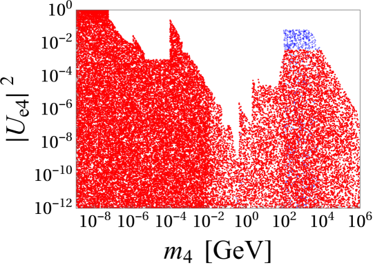
Figure 1: Result of the scan in the scenario of three active and one (effective) sterile neutrino, displayed in the plane $|U_{e4}|^{2}$ vs $m_{4}$. Perturbative unitarity cuts the parameter space for large $m_{4}$. The red points agree with all constraints while the blue ones are excluded by requiring the compatibility with experimental results for the leptonic $\tau$ decays.

For the purpose of this paper, in which we study the effects of an additional sterile neutrino on the kaon physics observables, the most interesting region is the one corresponding to $m_{4}\lesssim 1\;{\rm GeV}$, which we show in Fig. 2. As expected, the limits coming from the $\tau$ leptonic decays are the most constraining in the plane $(m_{4},|U_{\tau 4}|^{2})$. Notice also that the sharp exclusion of parameters around $m_{4}\sim 0.3\ {\rm GeV}$ comes from the direct searches discussed in Ref. [43]. It is worth noticing that the bounds shown in Fig. 2 are in agreement with those provided in Ref. [43] in the considered mass regime, although slightly improved as most of the constraints discussed above have been updated.

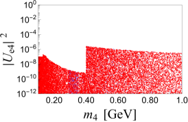
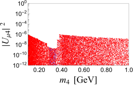
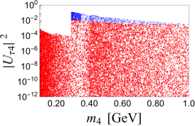
Figure 2: As in Fig. 1 but for $m_{4}\leq 1\leavevmode\nobreak\ {\rm GeV}$, and for all $|U_{\ell 4}|^{2}$.

In summary, we selected the points in the parameter space which are compatible with a number of constraints discussed in the body of this section. We will use the results of the above scan to test the sensitivity of the kaon physics observables on the presence of an effective massive sterile neutrino with a mass $m_{4}\lesssim 1$ GeV.

4 Kaon Physics Phenomenology

Before discussing the results stemming from our scan, we will introduce the kaon decays at the heart of our study and present their analytical expressions in our effective model. In our phenomenological discussion, we will consider the processes for which hadronic uncertainties are under full theoretical control by means of numerical simulations of QCD on the lattice. Processes such as $\mathcal{B}(K_{S}\to\mu\mu)$ and $\mathcal{B}(K\to\pi\mu\mu)$ will not be considered, since the corresponding Standard Model predictions depend on large (long-distance QCD) uncertainties.

4.1 Leptonic decays, $K_{\ell 2}$

Sterile neutrinos in kaon and pion leptonic decays were first studied and analyzed in [9] with the aim to probe massive neutrinos via lepton mixing; correspondingly, associated tests allowed one to set bounds on neutrino masses and lepton mixing matrix elements [10]. Here we revisit the $K_{\ell 2}$ decays in light of the existing data on neutrinos and in the framework of the simple extension of the Standard Model by one sterile fermion with the aim to update the latter obtained results.

The effective Hamiltonian we will be working with reads

$$\mathcal{H}_{\text{eff}}=\sqrt{2}G_{F}V_{us}\left[(1+g_{V})\,\bar{u}\gamma_{\mu}s\,\bar{\ell}_{L}\gamma^{\mu}\nu_{L}-(1+g_{A})\,\bar{u}\gamma_{\mu}\gamma_{5}s\,\bar{\ell}_{L}\gamma^{\mu}\nu_{L}+\mathrm{h.c.}\right]\,,$$ (38)

where $g_{A}$ and $g_{V}$ are the generic couplings to physics beyond the Standard Model, which in our case are the couplings to the massive sterile neutrino. The leptonic bilinear $\bar{\ell}_{L}\gamma^{\mu}\nu_{L}$ in Eq. (38) should be understood as $\sum_{\alpha=e,\mu,\tau}\operatornamewithlimits{\sum}_{i=1}^{3+N}U_{\alpha i}\,\bar{\ell}_{\alpha}\,\gamma^{\mu}\,P_{L}\,\nu_{i}\$, as in Eq. (1). In the effective approach, the effect of the active-sterile mixing is encoded in the effective couplings $g_{A}$ and $g_{V}$. The relevant hadronic matrix element for this decay is parametrized in terms of the decay constant $f_{K}$ via

$$\langle 0|\bar{u}\gamma_{\mu}\gamma_{5}s|K^{-}(p)\rangle=if_{K}p_{\mu},$$ (39)

so that the decay amplitude becomes

$$\mathcal{A}=-i\sqrt{2}G_{F}V_{us}(1+g_{A})(if_{K}p_{\mu})\bar{u}(k_{1})\gamma^{\mu}P_{L}v(k_{2})\,,$$ (40)

where $k_{1}$ and $k_{2}$ are the momenta of the lepton and neutrino, respectively, and $P_{L}=(1-\gamma_{5})/2$. Multiplying this amplitude by its conjugate and after summing over the spins we then get

$$\sum_{\mathrm{spin}}|\mathcal{A}|^{2}=2G_{F}^{2}|V_{us}|^{2}f_{K}^{2}|1+g_{A}|^{2}\left[m_{K}^{2}(m_{\ell}^{2}+m_{\nu}^{2})-(m_{\ell}^{2}-m_{\nu}^{2})^{2}\right],$$ (41)

so that the final expression for the decay rate reads

$${\mathcal{B}}(K\to\ell\nu_{i})={G_{F}^{2}\tau_{K}\over 8\pi m_{K}^{3}}|V_{us}|^{2}f_{K}^{2}\lambda^{1/2}(m_{K}^{2},m_{\ell}^{2},m_{\nu_{i}}^{2})|1+g_{A}|^{2}\left[m_{K}^{2}(m_{\ell}^{2}+m_{\nu_{i}}^{2})-(m_{\ell}^{2}-m_{\nu_{i}}^{2})^{2}\right]\,.$$ (42)

One can immediately see from the above equation (and the subsequent ones for the observables under this study) that the presence of the sterile state can have two consequences, a phase space effect if its mass is kinematically allowed and a modification of the coupling due to the active-sterile mixing encoded in $g_{A}$. More explicitly, and after adapting the above formula to the scenario with an extra sterile neutrino, we have

$${\mathcal{B}}(K\to\ell\nu)={G_{F}^{2}\tau_{K}\over 8\pi m_{K}^{3}}|V_{us}|^{2}f_{K}^{2}\sum_{i=1}^{4}|U_{\ell i}|^{2}\lambda^{1/2}(m_{K}^{2},m_{\ell}^{2},m_{\nu_{i}}^{2})\left[m_{K}^{2}(m_{\ell}^{2}+m_{\nu_{i}}^{2})-(m_{\ell}^{2}-m_{\nu_{i}}^{2})^{2}\right]\,.$$ (43)

Similarly, for the process $\tau\to K\nu$ we get

$${\mathcal{B}}(\tau\to K\nu)={G_{F}^{2}\tau_{\tau}\over 16\pi m_{\tau}^{3}}|V_{us}|^{2}f_{K}^{2}\sum_{i=1}^{4}|U_{\tau i}|^{2}\lambda^{1/2}(m_{\tau}^{2},m_{K}^{2},m_{\nu_{i}}^{2})\left[(m_{\tau}^{2}-m_{\nu_{i}}^{2})^{2}-m_{K}^{2}(m_{\tau}^{2}+m_{\nu_{i}}^{2})\right]\,.$$ (44)

The above expressions can be trivially extended to the case of the pion leptonic decay by simply replacing $K\to\pi$, and $V_{us}\to V_{ud}$. Modern day lattice QCD computations of the decay constants $f_{K}$, $f_{\pi}$, and especially of $f_{K}/f_{\pi}$, have already reached a subpercent accuracy [45] so that comparing the theoretical expressions (in which the effects of new physics are included) with the experimental measurements can result in stringent constraints on the new physics couplings.

4.2 Semileptonic decays, $K_{\ell 3}$

To discuss the semileptonic decays $K\to\pi\ell\nu$, we again rely on the effective Hamiltonian (38) and keep the neutrinos massive. Due to parity, only the vector current contributes on the hadronic side and the relevant hadronic matrix matrix element is parametrized as

$$\langle\pi^{+}(k)|\bar{u}\gamma_{\mu}s|\bar{K}^{0}(p)\rangle=\left(k_{\mu}+k_{\mu}-\frac{m_{K}^{2}-m_{\pi}^{2}}{q^{2}}q_{\mu}\right)f_{+}(q^{2})+\frac{m_{K}^{2}-m_{\pi}^{2}}{q^{2}}q_{\mu}\,f_{0}(q^{2})\,,$$ (45)

where the form factors $f_{+,0}(q^{2})$ are functions of $q^{2}=(p-k)^{2}=(k_{1}+k_{2})^{2}$ which can take the values $q^{2}\in[(m_{\ell}+m_{\nu})^{2},(m_{K}-m_{\pi})^{2}]$. Notice that the hadronic matrix element of the decay to a neutral pion is related to the above one by isospin symmetry, i.e. $\langle\pi^{0}(k)|\bar{u}\gamma_{\mu}s|{K}^{-}(p)\rangle=(1/\sqrt{2})\ \langle\pi^{+}(k)|\bar{u}\gamma_{\mu}s|\bar{K}^{0}(p)\rangle$. This decay is suitably described by its helicity amplitudes. To that end one first defines the polarization vectors of the virtual vector boson ($K\to\pi V^{\ast}$) as

$$\varepsilon_{\pm}^{\mu}=\frac{1}{\sqrt{q^{2}}}\left[0,\ \pm 1,\ -i,\ 0\right]^{T},\quad\varepsilon_{0}^{\mu}=\frac{1}{\sqrt{q^{2}}}\left[|\vec{q}|,\ 0,\ 0,\ -q^{0}\right]^{T},\quad\varepsilon_{t}^{\mu}=\frac{1}{\sqrt{q^{2}}}\left[q^{0},\ 0,\ 0,\ -|\vec{q}|\right]^{T},$$ (46)

so that the only nonzero helicity amplitudes will be $h_{0,t}(q^{2})=(1+g_{V})\varepsilon_{0,t}^{\mu\;\ast}\langle\pi^{+}(k)|\bar{u}\gamma_{\mu}s|\bar{K}^{0}(p)\rangle$, or explicitly

$$h_{0}(q^{2})={(1+g_{V})\over\sqrt{q^{2}}}\lambda^{1/2}(m_{K}^{2},q^{2},m_{\pi}^{2})f_{+}(q^{2})\,,\quad h_{t}(q^{2})={(1+g_{V})\over\sqrt{q^{2}}}\left(m_{K}^{2}-m_{\pi}^{2}\right)f_{0}(q^{2}).$$ (47)

In terms of these functions the decay amplitude reads

$$\mathcal{A}_{sl}=\sqrt{2}G_{F}V_{us}\left[-h_{0}(q^{2})\varepsilon_{\mu}^{0}+h_{t}(q^{2})\varepsilon_{\mu}^{t}\right]\;\bar{u}(k_{1})\gamma^{\mu}P_{L}v(k_{2})\,.$$ (48)

In the rest frame of the lepton pair the components of the vectors $k_{1}$ and $k_{2}$ of the final leptons are

$$k_{1}=(E_{\ell},p_{\ell}\sin\theta,0,p_{\ell}\cos\theta),\quad k_{2}=(E_{\nu},-p_{\ell}\sin\theta,0,-p_{\ell}\cos\theta),$$ (49)

where

$$E_{\ell}={q^{2}+m_{\ell}^{2}-m_{\nu}^{2}\over 2\sqrt{q^{2}}},\quad E_{\nu}={q^{2}-m_{\ell}^{2}+m_{\nu}^{2}\over 2\sqrt{q^{2}}},\quad p_{\ell}={\lambda^{1/2}(q^{2},m_{\ell}^{2},m_{\nu}^{2})\over 2\sqrt{q^{2}}}\,,$$ (50)

and $\theta$ is the angle between $\ell^{-}$ (in the lepton pair rest frame) and the flight direction of the leptonic pair (opposite to the pion direction) in the kaon rest frame. The decay rate can then be written as

$$\frac{d^{2}{\mathcal{B}}(K\to\pi\ell{\nu})}{dq^{2}\,d\cos\theta}=a(q^{2})+b(q^{2})\cos\theta+c(q^{2})\cos^{2}\theta\,,$$ (51)

where the $q^{2}$-dependent functions are given by

$$a(q^{2})= {G_{F}^{2}\tau_{K}\over 256\pi^{3}m_{K}^{3}}|V_{us}|^{2}\lambda^{1/2}(m_{K}^{2},q^{2},m_{\pi}^{2})\lambda^{1/2}(q^{2},m_{\ell}^{2},m_{\nu}^{2})$$

$$\times\left[\left(1-\frac{m_{\ell}^{2}+m_{\nu}^{2}}{q^{2}}\right)|h_{0}(q^{2})|^{2}+\left(\frac{m_{\ell}^{2}+m_{\nu}^{2}}{q^{2}}-\frac{(m_{\ell}^{2}-m_{\nu}^{2})^{2}}{q^{4}}\right)|h_{t}(q^{2})|^{2}\right],$$ (52)

$$b(q^{2})= {G_{F}^{2}\tau_{K}\over 128\pi^{3}m_{K}^{3}}|V_{us}|^{2}\lambda^{1/2}(m_{K}^{2},q^{2},m_{\pi}^{2})\lambda(q^{2},m_{\ell}^{2},m_{\nu}^{2})\frac{m_{\ell}^{2}-m_{\nu}^{2}}{q^{4}}\mathrm{Re}\left[h_{0}(q^{2})h_{t}^{\ast}(q^{2})\right],$$ (53)

$$c(q^{2})= -{G_{F}^{2}\tau_{K}\over 256\pi^{3}m_{K}^{3}}|V_{us}|^{2}\lambda^{1/2}(m_{K}^{2},q^{2},m_{\pi}^{2})\frac{\lambda^{3/2}(q^{2},m_{\ell}^{2},m_{\nu}^{2})}{q^{4}}|h_{0}(q^{2})|^{2}\,.$$ (54)

After integrating over $\theta$ we obtain the usual expression for the differential branching fraction, which is shortly written as

$$\frac{d{\mathcal{B}}(K\to\pi\ell\nu)}{dq^{2}}=2\,\left[a(q^{2})+\frac{1}{3}c(q^{2})\right]\,.$$ (55)

Finally, after integrating in $q^{2}$ and splitting up the pieces with contributions of massless and massive neutrinos in the final state, we have

$${\mathcal{B}}(K\to\pi\ell\nu)= (1-|U_{\ell 4}|^{2})\int\displaylimits_{m_{\ell}^{2}}^{(m_{K}-m_{\pi})^{2}}\left.\frac{d{\mathcal{B}}(K\to\pi\ell\nu)}{dq^{2}}\right|_{m_{\nu}=0}$$

$$+\vartheta\left(m_{K}-m_{\pi}-m_{\ell}-m_{4}\right)|U_{\ell 4}|^{2}\int\displaylimits_{(m_{\ell}+m_{4})^{2}}^{(m_{K}-m_{\pi})^{2}}\frac{d{\mathcal{B}}(K\to\pi\ell\nu_{4})}{dq^{2}}.$$ (56)

Another observable relevant to $K\to\pi\ell\nu$ decays can be easily obtained after subtracting the number of events in the backward from the forward hemispheres. The resulting forward-backward asymmetry is given by

$$\!\!\!A_{\rm fb}^{\ell}(q^{2})={\displaystyle{\int_{0}^{1}d\cos\theta\frac{d^{2}{\mathcal{B}}(K\to\pi\ell\nu)}{dq^{2}\,d\cos\theta}}-\int_{-1}^{0}d\cos\theta\displaystyle{\frac{d^{2}{\mathcal{B}}(K\to\pi\ell\nu)}{dq^{2}\,d\cos\theta}}\over\displaystyle{\int_{-1}^{1}d\cos\theta\frac{d^{2}{\mathcal{B}}(K\to\pi\ell\nu)}{dq^{2}\,d\cos\theta}}}\;.$$ (57)

Since there are three independent functions in the angular decay distribution (51) we can define one more linearly independent observable, in addition to $d{\mathcal{B}}/dq^{2}$ and $A_{\rm fb}(q^{2})$. We choose the third observable to be the charged lepton polarization asymmetry. For that purpose we define the projectors $P_{\pm}=(1\pm\not{s}\gamma_{5})/2$ where the projection is made along the lepton polarization vector,

$$s=\left(\frac{|\vec{p}_{\ell}|}{m_{\ell}},\frac{E_{\ell}}{m_{\ell}}\frac{\vec{p}_{\ell}}{|\vec{p}_{\ell}|}\right)\,.$$ (58)

The differential branching fraction can be separated into the positive lepton helicity and the negative one, i.e.

$$\frac{d{\mathcal{B}}(K\to\pi\ell\nu)}{dq^{2}} =\frac{d{\mathcal{B}}_{+}(K\to\pi\ell\nu)}{dq^{2}}+\frac{d{\mathcal{B}}_{-}(K\to\pi\ell\nu)}{dq^{2}},$$ (59)

or, for short, ${\mathcal{B}}={\mathcal{B}}_{+}+{\mathcal{B}}_{-}$. The lepton polarization asymmetry is then defined as

$$P_{\ell}(q^{2})={\quad\displaystyle{\frac{d{\mathcal{B}}_{+}}{dq^{2}}}-\displaystyle{\frac{d{\mathcal{B}}_{-}}{dq^{2}}}\quad\over\displaystyle{\frac{d{\mathcal{B}}_{+}}{dq^{2}}}+\displaystyle{\frac{d{\mathcal{B}}_{-}}{dq^{2}}}}= {1\over\displaystyle{(d{\mathcal{B}}/dq^{2})}}{G_{F}^{2}\tau_{K}\over 384\pi^{3}m_{K}^{3}}|V_{us}|^{2}\lambda^{1/2}(m_{K}^{2},q^{2},m_{\pi}^{2}){\lambda(q^{2},m_{\ell}^{2},m_{\nu}^{2})\over q^{2}}$$

$$\times\left[\left(-2+\frac{m_{\ell}^{2}-m_{\nu}^{2}}{q^{2}}\right)|h_{0}(q^{2})|^{2}+3\frac{m_{\ell}^{2}-m_{\nu}^{2}}{q^{2}}|h_{t}(q^{2})|^{2}\right]\,,$$ (60)

or, in terms of form factors and by explicitly displaying the sum over the neutrino species, we write

$$P_{\ell}(q^{2})= {1\over\displaystyle{(d{\mathcal{B}}/dq^{2})}}{G_{F}^{2}\tau_{K}\over 192\pi^{3}m_{K}^{3}}|V_{us}|^{2}{\lambda^{1/2}(m_{K}^{2},q^{2},m_{\pi}^{2})\over q^{4}}\sum_{i=1}^{4}|U_{\ell i}|^{2}\lambda(q^{2},m_{\ell}^{2},m_{\nu_{i}}^{2})$$

$$\times\left[\lambda(m_{K}^{2},q^{2},m_{\pi}^{2})\left(\frac{m_{\ell}^{2}-m_{\nu_{i}}^{2}}{2q^{2}}-1\right)|f_{+}(q^{2})|^{2}+\frac{3}{2}\frac{m_{\ell}^{2}-m_{\nu_{i}}^{2}}{q^{2}}(m_{K}^{2}-m_{\pi}^{2})^{2}|f_{0}(q^{2})|^{2}\right].$$ (61)

Measuring $A_{\rm fb}^{\ell}(q^{2})$ and $P_{\ell}(q^{2})$ is hardly possible, but measuring the integrated characteristics might be feasible. This is why in the phenomenological application we will be using $\langle A_{\rm fb}^{\ell}\rangle$ and $\langle P_{\ell}\rangle$, which are obtained by separately integrating the numerator and the denominator in both Eqs. (57) and (4.2).

4.3 Loop-induced weak decay $K\to\pi\nu\nu$

Details of the derivation of the expressions for this decay rate can be found in Appendix (A.2) of the present paper. Here we only quote the corresponding effective Hamiltonian that we use, namely,

$$\mathcal{H}_{\text{eff}}=\frac{\sqrt{2}G_{F}\alpha_{\mathrm{em}}}{\pi}\sum_{i,j=1}^{4}{\widetilde{C}}_{L}^{ij}\left(\bar{s}\gamma_{\mu}P_{L}d\right)\left(\nu_{i}\gamma^{\mu}P_{L}\nu_{j}\right)+\mathrm{h.c.}$$ (62)

where

$$\widetilde{C}_{L}^{i,j}=\frac{1}{\sin^{2}\theta_{W}}\sum_{\ell\in\{e,\mu,\tau\}}U_{\ell i}^{\ast}\left[\lambda_{c}X_{c}^{\ell}+\lambda_{t}X_{t}\right]U_{\ell j}\,,$$ (63)

with $\lambda_{c}=V_{cs}^{\ast}V_{cd}$, $\lambda_{t}=V_{ts}^{\ast}V_{td}$. The loop contribution arising from the top quark amounts to $X_{t}=1.47(2)$ [46], while the box diagram with the propagating charm depends on the lepton also in the loop, and yields $X_{c}^{e}=X_{c}^{\mu}=10.0(7)\times 10^{-4}$, $X_{c}^{\tau}=6.5(6)\times 10^{-4}$ [47]. Notice also that the sum in the Wilson coefficient $\widetilde{C}_{L}^{i,j}$ runs over the charged lepton species and the one in Eq. (62) over the neutrino mass eigenstates. Using the same decomposition of the matrix element in terms of the hadronic form factors, already defined in Eq. (45), and assuming all neutrinos to be of Majorana nature, we have

$$\frac{d{\mathcal{B}}(K^{+}\to\pi^{+}\nu\nu)}{dq^{2}}= \mathop{\sum_{i,j=1}^{4}}_{i\leq j}\left(1-\frac{1}{2}\delta_{ij}\right){\alpha_{\mathrm{em}}^{2}G_{F}^{2}\tau_{K^{+}}\over 768\pi^{5}m_{K}^{3}}\lambda^{1/2}(m_{K}^{2},q^{2},m_{\pi}^{2}){\lambda^{1/2}(q^{2},m_{\nu_{i}}^{2},m_{\nu_{j}}^{2})\over q^{2}}$$

$$\times\left\{|\widetilde{C}_{L}^{ij}|^{2}\left[\lambda(m_{K}^{2},q^{2},m_{\pi}^{2})\left(2-\frac{m_{\nu_{i}}^{2}+m_{\nu_{j}}^{2}}{q^{2}}-\frac{(m_{\nu_{i}}^{2}-m_{\nu_{j}}^{2})^{2}}{q^{4}}\right)|f_{+}(q^{2})|^{2}\right.\right.$$

$$\qquad\left.+3\left(\frac{m_{\nu_{i}}^{2}+m_{\nu_{j}}^{2}}{q^{2}}-\frac{(m_{\nu_{i}}^{2}-m_{\nu_{j}}^{2})^{2}}{q^{4}}\right)(m_{K}^{2}-m_{\pi}^{2})^{2}|f_{0}(q^{2})|^{2}\right]$$

$$\left.-6\frac{m_{i}m_{j}}{q^{2}}\widehat{C}_{L}^{ij}\left[\lambda(m_{K}^{2},q^{2},m_{\pi}^{2})|f_{+}(q^{2})|^{2}-(m_{K}^{2}-m_{\pi}^{2})^{2}|f_{0}(q^{2})|^{2}\right]\right\},$$ (64)

where

$$\widehat{C}^{ij}_{L}=\frac{1}{\sin^{4}\theta_{W}}\sum_{\ell,\ell^{\prime}\in\{e,\mu,\tau\}}\left(\lambda_{c}X_{c}^{\ell}+\lambda_{t}X_{t}\right)\left(\lambda_{c}X_{c}^{\ell^{\prime}}+\lambda_{t}X_{t}\right)^{\ast}\times\mathrm{Re}\left[U_{\ell i}^{\ast}U_{\ell j}U_{\ell^{\prime}i}^{\ast}U_{\ell^{\prime}j}\right]\,.$$ (65)

One should be particularly careful when using the above formula because the leptonic mixing matrix elements are in general complex, and while the functions $X_{c}^{\ell}$ and $X_{t}$ are real, the Cabibbo-Kobayashi-Maskawa couplings have both real and imaginary parts. More specifically, and by using the CKMfitter results [48], we obtain

$$\mathrm{Re}\lambda_{t}=-3.31(9)\times 10^{-4},\quad\mathrm{Re}\lambda_{c}=-0.2193(3),\quad\mathrm{Im}\lambda_{t}=-\mathrm{Im}\lambda_{c}=1.38(5)\times 10^{-4}.$$ (66)

The above formula reduces to the Standard Model one after setting $m_{\nu_{i}}=m_{\nu_{j}}=0$, and by using the unitarity of the $4\times 4$ matrix.

If this decay occurs between the neutral mesons, the situation is slightly more delicate. When considering $K_{L}\to\pi^{0}\nu\nu$, one should first keep in mind that $|K_{L}\rangle=(|K^{0}\rangle+|\overline{K}^{0}\rangle)/\sqrt{2}$, which then means that the effective Hamiltonian (62) between the initial and the final hadrons will result in two hadronic matrix elements which are related to each other by CP symmetry, namely,

$$\langle\pi^{0}|\bar{d}\gamma_{\mu}s|\overline{K}^{0}\rangle=-\langle\pi^{0}|\bar{s}\gamma_{\mu}d|K^{0}\rangle.$$ (67)

Furthermore, after invoking the isospin symmetry, we have

$$\langle\pi^{0}|\bar{s}\gamma_{\mu}d|K^{0}\rangle=\langle\pi^{0}|\bar{s}\gamma_{\mu}u|K^{+}\rangle=\frac{1}{\sqrt{2}}\langle\pi^{+}|\bar{s}\gamma_{\mu}u|\overline{K}^{0}\rangle,$$ (68)

where the last matrix element (to a charged pion) is the one defined in Eq. (45). With this, we can compute the decay rate and we obtain

$$\frac{d{\mathcal{B}}(K_{L}\to\pi^{0}\nu\nu)}{dq^{2}}= \mathop{\sum_{i,j=1}^{4}}_{i\leq j}\left(1-\frac{1}{2}\delta_{ij}\right){\alpha_{\mathrm{em}}^{2}G_{F}^{2}\tau_{K_{L}}\over 768\pi^{5}m_{K}^{3}}\lambda^{1/2}(m_{K}^{2},q^{2},m_{\pi}^{2}){\lambda^{1/2}(q^{2},m_{\nu_{i}}^{2},m_{\nu_{j}}^{2})\over q^{2}}$$

$$\times\left\{|\widetilde{C}_{0}^{ij}|^{2}\left[\lambda(m_{K}^{2},q^{2},m_{\pi}^{2})\left(2-\frac{m_{\nu_{i}}^{2}+m_{\nu_{j}}^{2}}{q^{2}}-\frac{(m_{\nu_{i}}^{2}-m_{\nu_{j}}^{2})^{2}}{q^{4}}\right)|f_{+}(q^{2})|^{2}\right.\right.$$

$$\qquad\left.+3\left(\frac{m_{\nu_{i}}^{2}+m_{\nu_{j}}^{2}}{q^{2}}-\frac{(m_{\nu_{i}}^{2}-m_{\nu_{j}}^{2})^{2}}{q^{4}}\right)(m_{K}^{2}-m_{\pi}^{2})^{2}|f_{0}(q^{2})|^{2}\right]$$

$$\left.-6\frac{m_{i}m_{j}}{q^{2}}\widehat{C}_{0}^{ij}\left[\lambda(m_{K}^{2},q^{2},m_{\pi}^{2})|f_{+}(q^{2})|^{2}-(m_{K}^{2}-m_{\pi}^{2})^{2}|f_{0}(q^{2})|^{2}\right]\right\},$$ (69)

where

$$\widetilde{C}_{0}^{i,j}=-\frac{1}{\sin^{2}\theta_{W}}\sum_{\ell\in\{e,\mu,\tau\}}U_{\ell i}^{\ast}\mathrm{Im}\left[\lambda_{c}X_{c}^{\ell}+\lambda_{t}X_{t}\right]U_{\ell j},$$

$$\widehat{C}^{ij}_{0}=\frac{1}{\sin^{4}\theta_{W}}\sum_{\ell,\ell^{\prime}\in\{e,\mu,\tau\}}\mathrm{Im}\left(\lambda_{c}X_{c}^{\ell}+\lambda_{t}X_{t}\right)\mathrm{Im}\left(\lambda_{c}X_{c}^{\ell^{\prime}}+\lambda_{t}X_{t}\right)\mathrm{Re}\left[U_{\ell i}^{\ast}U_{\ell j}U_{\ell^{\prime}i}^{\ast}U_{\ell^{\prime}j}\right].$$ (70)

Like before, if we set $m_{\nu_{i}}=m_{\nu_{j}}=0$ and use the $U$ matrix unitarity, the above formula will lead to the familiar Standard Model expression (see e.g. [47]).

4.4 “Invisible decay” $K_{L}\to\nu\nu$

One might also look for an “invisible decay”, such as the decay of a kaon to neutrinos only. We use the effective Hamiltonian (62), and express the hadronic matrix element as

$$\langle 0|\bar{s}\gamma_{\mu}\gamma_{5}d|K_{L}(p)\rangle=\langle 0|\bar{d}\gamma_{\mu}\gamma_{5}s|K_{L}(p)\rangle=\frac{i}{\sqrt{2}}f_{K}p_{\mu},$$ (71)

consistent with Eq. (39), and derive the expression for the decay rate by keeping in mind that $CP|K^{0}\rangle=-|\overline{K}^{0}\rangle$. We obtain

$${\mathcal{B}}(K_{L}\to\nu\nu) =\mathop{\sum_{i,j=1}^{4}}_{i\leq j}\left(1-\frac{1}{2}\delta_{ij}\right)\frac{\alpha_{\rm em}^{2}G_{F}^{2}\tau_{K_{L}}}{8\pi^{3}m_{K}^{3}\sin^{4}\theta_{W}}f_{K}^{2}\lambda^{1/2}(m_{K}^{2},m_{\nu_{i}}^{2},m_{\nu_{j}}^{2})$$

$$\times\left[\biggl{|}\sum_{\ell\in\{e,\mu,\tau\}}\!\!\mathrm{Re}\left(\lambda_{c}X_{c}^{\ell}+\lambda_{t}X_{t}\right)U_{\ell i}^{\ast}U_{\ell j}\biggr{|}^{2}\left(m_{K}^{2}(m_{\nu_{i}}^{2}+m_{\nu_{j}}^{2})-(m_{\nu_{i}}^{2}-m_{\nu_{j}}^{2})^{2}\right)\right.$$

$$\left.+\ 2\!\!\sum_{\ell,\ell^{\prime}\in\{e,\mu,\tau\}}\!\!\mathrm{Re}(\lambda_{c}X_{c}^{\ell}+\lambda_{t}X_{t})\mathrm{Re}(\lambda_{c}X_{c}^{\ell^{\prime}}+\lambda_{t}X_{t})\mathrm{Re}(U_{\ell i}^{\ast}U_{\ell j}U_{\ell^{\prime}i}^{\ast}U_{\ell^{\prime}j})\;m_{\nu_{i}}m_{\nu_{j}}m_{K}^{2}\right].$$ (72)

Since we consider the neutrinos to be Majorana fermions, the processes $K\to\pi\nu\nu$ and $K_{L}\to\nu\nu$ can be viewed as lepton number violating, and as such they can be used to probe the Majorana phases via the last term in Eqs. (4.3) and (4.4). Notice, however, that this term is multiplied by the product of neutrino masses $m_{\nu_{i}}m_{\nu_{j}}$, and since in our scenario only one neutrino can be massive the other ones are extremely light so that the product of masses will be negligibly small. The only nonzero possibility is then $i=j=4$, but in this case the Majorana phases cancel out in the product $U_{\ell 4}^{\ast}U_{\ell 4}U_{\ell^{\prime}4}^{\ast}U_{\ell^{\prime}4}$. For this reason, the Majorana phases will not be discussed in what follows. We should also note that Eq. (4.4), with the appropriate simplifications, agrees with the one presented in Ref. [49].

5 Results and discussion

In this section we use the points selected by the constraints discussed in Sec. 3 and evaluate the sensitivity of the kaon decay observables on the presence of a massive sterile neutrino. Whenever possible, and to make the situation clearer, for a given observable $\mathcal{O}$ we will consider the ratio

$$R_{\mathcal{O}}=\frac{\mathcal{O}}{\mathcal{O}^{\mathrm{SM}}}\,,$$ (73)

where in the numerator we compute a given observable in the scenario with three active and one massive sterile neutrino and divide it by its Standard Model prediction. Whenever possible, those results will be compared with experimental values, $R_{\mathcal{O}}^{\mathrm{exp}}$.

$\bullet$ We first examine the effects of sterile neutrinos on the leptonic decays of a charged kaon. To that end we define

$$R_{K\ell 2}=\frac{{\mathcal{B}}(K\to\ell\nu)}{{\mathcal{B}}(K\to\ell\nu)^{\mathrm{SM}}},$$ (74)

and compute its value by employing the expressions derived in the previous section. To estimate $R_{K\ell 2}^{\mathrm{exp}}$ we need an estimate of ${\mathcal{B}}(K\to\ell\nu)^{\mathrm{SM}}$, which we compute by using $|V_{us}|=0.2255(4)$ [48], $f_{K}=155.6(4)$ MeV computed in lattice QCD [45], and by adding the electroweak and radiative corrections [50, 51, 52]. We thus end up with

$${\mathcal{B}}(K^{+}\to e^{+}\nu)^{\mathrm{SM}} =1.572(10)\times 10^{-5}, R_{Ke2}^{\mathrm{exp}} =1.006(8)\,,$$

$${\mathcal{B}}(K^{+}\to\mu^{+}\nu)^{\mathrm{SM}} =63.55(39)\%, R_{K\mu 2}^{\mathrm{exp}} =0.999(6)\,,$$

$${\mathcal{B}}(\tau^{+}\to K^{+}\nu)^{\mathrm{SM}} =7.14(4)\times 10^{-3}, R_{\tau K2}^{\mathrm{exp}} =0.980(15)\,,$$ (75)

where, in evaluating the $R_{K\ell 2}^{\mathrm{exp}}$ ratios, we used the average of the experimental results collected in Ref. [38].

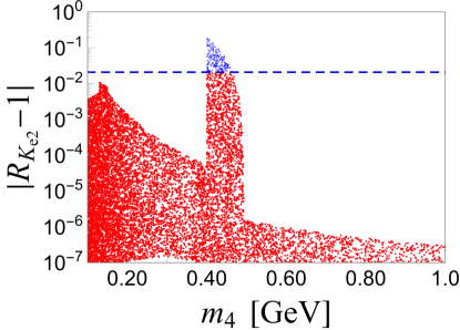
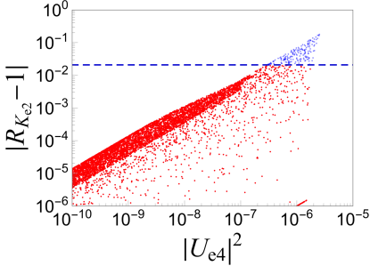
Figure 3: $|R_{Ke2}-1|$ as a function of the sterile neutrino mass, $m_{4}$ (left panel) and of $U_{e4}$ (right panel). The full ensemble of points (red and blue ones) correspond to $R_{Ke2}$ computed using Eq. (43) in the Standard Model and in our scenario, with an additional sterile neutrino, by using the parameters selected in the scan discussed in Sec. 3. Blue points are in conflict with $R_{Ke2}^{\mathrm{exp}}$ shown by the dashed line.

Adding a massive sterile neutrino with parameters selected in a way discussed in Sec. 3, results in values of the branching fractions which always fall within the experimental bounds except in the case of the mode $K\to e\nu$, where some points get outside the range allowed by experiment. This situation is depicted in Fig. 3 where we see that requiring an agreement with the experimental bound on $R_{Ke2}$ amounts to a new constraint in the region of $m_{4}\in(400\;{\rm MeV},m_{K})$. In Fig. 3 we also show the impact of $R_{Ke2}^{\mathrm{exp}}$ on the corresponding active-sterile mixing angle, or better $U_{e4}$.

This finding is actually equivalent to what has been discussed in Ref. [40] where it has been shown that $\Delta r_{K}$ (defined analogously to Eq. (28) of the present paper) provides a useful constraint when building a viable extension of the Standard Model by including one (or more) sterile neutrino(s). Knowing that

$$\Delta r_{K}={R_{Ke2}\over R_{K\mu 2}}-1\,,$$ (76)

and since $R_{Ke2}$ is currently constraining while $R_{K\mu 2}$ is not, it is clear that the two constraints are indeed equivalent.

$\bullet$ As for the semileptonic decays, we focus on the decays of $K_{L}$ in order to avoid the uncertainties related to the isospin corrections which are present in the decays of charged kaons. The main remaining worry is to handle the hadronic uncertainties, i.e. those associated with the form factors $f_{+,0}(q^{2})$. Those uncertainties are nowadays under control thanks to the recent precision lattice QCD computation with $N_{\mathrm{f}}=2+1+1$ dynamical quark flavors, presented in Ref. [53]. In that paper the authors computed the form factors at several $q^{2}$’s which are then fitted to the dispersive parametrization of Ref. [54]. We use those results in our computation and obtain,

$${\mathcal{B}}(K_{L}\to\pi^{-}e^{+}\nu)^{\mathrm{SM}} =41.31(46)\%, R_{Ke3}^{\mathrm{exp}} =0.980(13)\,,$$

$${\mathcal{B}}(K_{L}\to\pi^{-}\mu^{+}\nu)^{\mathrm{SM}} =27.51(29)\%, R_{K\mu 3}^{\mathrm{exp}} =0.981(11)\,,$$ (77)

thus about $1.5\sigma$ away from the Standard Model prediction. Those bounds, however, remain far too above the results we obtain after including an extra sterile neutrino, which is also shown in Fig. 4. In other words, the presence of a massive sterile neutrino has a very little impact on the branching fractions of the semileptonic kaon decays $K_{\ell 3}$. Even a significantly increased precision of those measurements is very unlikely to unveil the presence of a sterile neutrino in these decay modes.

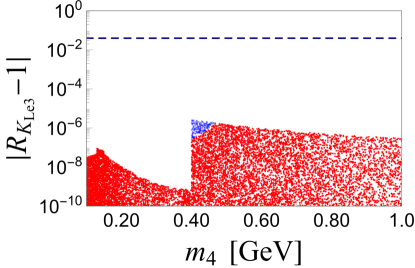
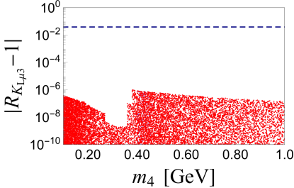
Figure 4: Predictions for $|R_{Ke3}-1|$ and $|R_{K\mu 3}-1|$, computed by using the parameters obtained in Sec. 3, are shown as functions of the mass of the sterile neutrino $m_{4}$. All the allowed points in red remain far below the experimental limit, shown by the dashed line. Blue points correspond to those discarded by incompatibility with $R_{Ke2}^{\mathrm{exp}}$.

As for the other two observables, we first computed them in the Standard Model and obtained

$$K_{L}\to\pi e\nu: \langle A_{\mathrm{fb}}^{e}\rangle^{\mathrm{SM}} =8.5(1)\times 10^{-5}, \langle P_{e}\rangle^{\mathrm{SM}} =0.999(16),$$

$$K_{L}\to\pi\mu\nu: \langle A_{\mathrm{fb}}^{\mu}\rangle^{\mathrm{SM}} =0.271(4), \langle P_{\mu}\rangle^{\mathrm{SM}} =0.088(5).$$ (78)

We then checked their values in our scenario with one massive sterile neutrino and found that they change by a completely insignificant amount (at the one per-mil level). For example, we get

$$-2\times 10^{-7}\leq \left(\langle A_{\mathrm{fb}}^{\mu}\rangle-\langle A_{\mathrm{fb}}^{\mu}\rangle^{\mathrm{SM}}\right)\leq 5\times 10^{-7}$$

$$-3.6\times 10^{-6}\leq \left(\langle P_{\mu}\rangle-\langle P_{\mu}\rangle^{\mathrm{SM}}\right)\leq 2.3\times 10^{-6}.$$ (79)

To understand why these quantities remain so insensitive to the presence of a heavy sterile neutrino, we checked all the constraints employed in our scan of parameters, and found that the most severe constraints come from the direct searches, i.e. those we took from Ref. [43]. Once taken into account, these constraints prevent the kaon physics observables from deviating from their Standard Model values.

$\bullet$ The most interesting decay modes are expected to be the ones with two neutrinos in the final state. In the Standard Model, we have [55]

$${\mathcal{B}}^{\mathrm{SM}}(K_{L}\to\pi^{0}\nu\nu)=(3.00\pm 0.30)\times 10^{-11},$$

$${\mathcal{B}}^{\mathrm{SM}}(K^{\pm}\to\pi^{\pm}\nu\nu)=(9.11\pm 0.72)\times 10^{-11},$$ (80)

where a control over the remaining long-distance hadronic contribution to the charged mode can be achieved through numerical simulations of QCD on the lattice for which a strategy has been recently developed in Ref. [56]. These two decay modes are also subjects of an intense experimental research at CERN (NA62) for the charged mode [11], and at J-PARC (KOTO) for the neutral one [12]. We therefore find it important to examine in which way their rates could be affected if the Standard Model is extended by an extra sterile neutrino. It turns out that experimental constraints limit the deviation from the Standard Model prediction to less than $1\%$, which in view of the Standard Model uncertainties [cf. Eq. (5)] means that the $K\to\pi\nu\nu$ decay modes remain blind to the presence of an extra sterile neutrino. This is illustrated in Fig. 5.

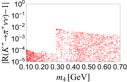
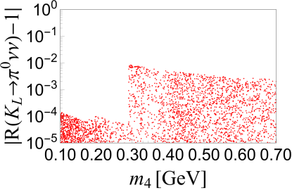
Figure 5: $|R_{K^{\pm}\to\pi^{\pm}\nu\nu}-1|$ and $|R_{K_{L}\to\pi^{0}\nu\nu}-1|$ remain within $1\%$, which means that $K\to\pi\nu\nu$ decays are not sensitive to the presence of an extra (massive) sterile neutrino once experimental constraints are applied.

More specifically, we find

$$\forall\ m_{4}\leq 1\ {\rm GeV}\,,\qquad R_{K_{L}\to\pi^{0}\nu\nu}=1.000(9),\quad R_{K^{\pm}\to\pi^{\pm}\nu\nu}=1.000(8)\,.$$ (81)

In other words, measuring ${\mathcal{B}}(K_{L}\to\pi^{0}\nu\nu)$ and ${\mathcal{B}}(K^{\pm}\to\pi^{\pm}\nu\nu)$ consistent with the Standard Model predictions would be perfectly consistent with a scenario in which the Standard Model is extended by an extra sterile neutrino. Notice again that the cut into the parameter space in the region around $m_{4}\approx 0.29$ GeV – shown in Fig. 5 – comes from the direct searches [43], implemented in our scan.

$\bullet$ Finally, a similar analysis of the “invisible kaon decay” $K_{L}\to\nu\nu$ shows that this mode can be largely enhanced if the sterile neutrino is massive. Due to the available phase space, this decay can be studied for $m_{4}\leq m_{K^{0}}$, and the result is shown in Fig. 6.

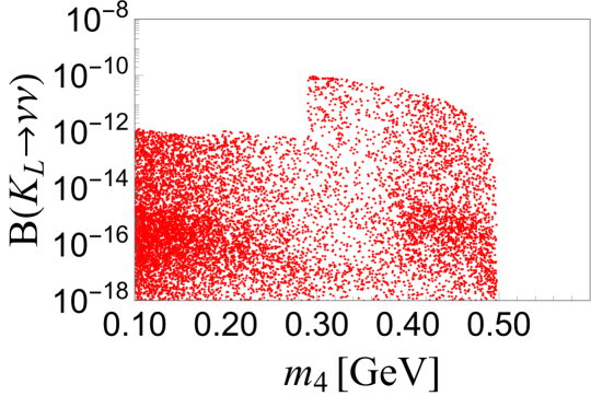
Figure 6: ${\mathcal{B}}(K_{L}\to\nu\nu)$ as a function of mass of the sterile neutrino for $m_{4}\leq m_{K^{0}}$. Notice that in the Standard Model this branching fraction is zero while the values close to the upper bound found here are possibly within the reach of the KOTO, NA62(-KLEVER) and SHIP experiments.

Knowing that in the Standard Model ${\mathcal{B}}(K_{L}\to\nu\nu)^{\mathrm{SM}}\approx 0$, the enhancement we observe is indeed substantial and since its decay rate can be comparable to ${\mathcal{B}}(K\to\pi\nu\nu)$ its experimental research becomes highly important. It has been proposed to search for this decay at the NA64 experiment using $K_{L}$ produced from a $K^{+}$ beam hitting a target [13]. From our analysis we find the upper bound,

$${\mathcal{B}}(K_{L}\to\nu\nu)\leq 1.2\times 10^{-10},$$ (82)

which could be within the reach of the KOTO, NA62(-KLEVER) and SHIP experiments even if the above bound is by an order of magnitude lower. The KOTO experiment aims to reach a sensitivity of $10^{-11}$ to $K_{L}\rightarrow\pi^{0}\nu\nu$ in its first phase [12] and to have $4\times 10^{14}\,K_{L}$ at the entrance of the detector in phase 2 [57]. NA62-KLEVER is a project that would succeed NA62 and would aim to produce $3\times 10^{13}\,K_{L}$ [58]. However, we would like to point out that the decay $K_{L}\to\nu\nu$ could also be searched for in $D$-meson decays, making use of the relatively large branching ratio ${\mathcal{B}}(D\to K_{L}\pi)\sim 1\%$ and tagging the $K_{L}$ via the pion. Beam dumps experiments at the CERN SPS like SHIP or a possible run of NA62 in a beam dump configuration would produce copious amounts of $D$ mesons. A year of running in beam dump mode for NA62 would produce $\sim 10^{15}\,D$ mesons [59], which would correspond to roughly $10^{13}$ tagged $K_{L}$. SHIP would accumulate even more data, producing $6.8\times 10^{17}\,D$ mesons [17], which would translate into more than $7\times 10^{15}$ tagged $K_{L}$. In any case, an experimental bound on this decay mode would be of great importance for studying the effects of physics beyond the Standard Model in the leptonic sector. Obviously, a nonzero measurement of ${\mathcal{B}}(K_{L}\to\nu\nu)$ would be a clean signal of the non-Standard Model physics.

Before closing this section, we should make a brief comment on the lepton flavor violating kaon decays, which in our scenario would be generated by the heavy neutrino running in the loop. By using the formulas given in Ref. [60] trivially adapted to the kaon decays, and the result of the scan of Sec. 3, we obtain that these modes are completely negligible, i.e. the branching fractions of all these modes are under $10^{-16}$. 

6 Summary

In this paper we presented the results of our study concerning the impact of a massive sterile neutrino on the weak kaon decays such as the leptonic, semileptonic and the decay of a kaon to neutrinos. In the effective approach adopted in this work, one sterile neutrino is supposed to mimic the effect of a more realistic model in which the neutrino sector is extended to include one or more sterile neutrinos.

Although the mass of the sterile neutrino $m_{4}$ can in principle have any value, we focused on the mass range $m_{4}\in[0,1]$ GeV, and in particular on $m_{4}\leq m_{K}$, when the sterile neutrino is kinematically accessible. In order to constrain six new parameters ($m_{4}$, the three sterile-active neutrino mixing angles and two new phases) we used a number of quantities discussed in the body of the paper, together with the perturbative unitarity requirement, as well as the constraints arising from the direct searches [43]. After combining such selected parameters with the expressions for the leptonic and semileptonic decays we derive here, we found that only $\mathcal{B}(K\to e\nu)$ can significantly deviate from the current experimental value. That conflict with the data is present in the interval $m_{K}>m_{4}\gtrsim 0.4$ GeV. The other quantities, including the forward backward and the lepton polarization asymmetries, remain unchanged with respect to their Standard Model values with the effect of the massive sterile neutrino remaining at the level of less than $1\%$.

We also derived the expressions for the kaon decays to two (Majorana) neutrinos in the final state, namely ${\mathcal{B}}(K\to\pi\nu\nu)$ and ${\mathcal{B}}(K_{L}\to\nu\nu)$. Our expressions are generic and can be used when studying a new physics scenario in which heavy neutrinos with no new gauge couplings are involved. This will be increasingly relevant with the ongoing experimental effort at CERN (NA62, NA64, SHIP) and J-PARC (KOTO) targeting $\mathcal{B}(K^{\pm}\to\pi^{\pm}\nu\nu)$ and $\mathcal{B}(K_{L}\to\pi^{0}\nu\nu)$, respectively. These two decays, however, appear to be insensitive to the massive sterile neutrino once the experimental and theoretical constraints are taken into account. In other words, if the experimental results of the weak kaon decays turn out to be consistent with the Standard Model predictions to a $1\%$ uncertainty, this would not be in contradiction with the neutrino sector extended by a massive and relatively light sterile neutrino(s). The only kaon decay mode which appears to be sensitive to the presence of a massive sterile neutrino is $K_{L}\to\nu\nu$, the branching fraction of which can go up to $\mathcal{O}(10^{-10})$, thus possibly within reach of the NA62(-KLEVER), SHIP and KOTO experiments. Knowing that the Standard Model value of this mode is zero, its observation would be a clean signal of new physics.

Notice also that ${\mathcal{B}}(K\to\pi\nu\nu)$ and ${\mathcal{B}}(K_{L}\to\nu\nu)$ could be used to probe the Majorana phases in the models in which more than one massive neutrino is considered. In the approach adopted in this paper only one neutrino can be heavy and therefore such a study is prohibited. If instead one considers a realistic model with more than one heavy neutrino then a study of the Majorana phases becomes possible too [61].

We should mention that one can also consider the situation with a very heavy sterile neutrino ${\mathcal{O}}(1\,\mathrm{TeV})$. In that case the processes discussed in this paper could be modified by the effects of violation of the mixing matrix unitarity; see for instance[62]. We checked that possibility in the explicit computation and found that such effects are indeed tiny. Importantly, however, a heavy sterile neutrino can propagate in the loop-induced processes and shift the values of ${\mathcal{B}}(K_{S}\to\mu\mu)$ and ${\mathcal{B}}(K\to\pi\mu\mu)$. We checked that the corresponding effect remains small and completely drowned in the large (long-distance QCD) uncertainties already present in the Standard Model estimates of ${\mathcal{B}}(K_{S}\to\mu\mu)$ and ${\mathcal{B}}(K\to\pi\mu\mu)$ [52, 63].

Finally, the expressions presented in this paper can be easily extended to other similar decays, such as $D$-, $D_{s}$-, $B$- and $B_{s}$-meson decays. We decided to focus on the kaon decays because of the recent theoretical developments in taming the hadronic uncertainties and because of the better experimental precision.

Acknowledgments: We thank S. Gninenko (spokesperson of NA64) for very interesting remarks.This project has received funding from the European Union’s Horizon 2020 research and innovation program under the Marie Sklodowska-Curie Grants No. 690575 and No. 674896. C.W. receives financial support from the European Research Council under the European Union’s Seventh Framework Programme (Grants No. FP/2007-2013)/ERC Grant NuMass Grant No. 617143. C.W. thanks the Université Paris Sud, the University of Tübingen and the IBS Center for Theoretical Physics of the Universe for their hospitality during the final stages of this project. R.Z.F. thanks the Université Paris Sud for the kind hospitality, and CNPq and FAPESP for partial financial support.

Appendix A Majorana vs Dirac case

Being electrically neutral neutrinos can be described by using either Dirac or Majorana spinors. A Majorana spinor obeys the condition

$$\psi=\psi^{C}=\xi\,\mathcal{C}\bar{\psi}^{T}\,,$$ (83)

where $C$ denotes the charge conjugation and $\xi$ an arbitrary phase factor that can be absorbed into redefinition of $\psi$. As a consequence, a Majorana spinor has only 2 degrees of freedom (whereas a Dirac spinor has 4) and can be expressed using only the left-handed (LH) chiral component

$$\psi=\psi_{L}+(\psi_{L})^{C}\,.$$ (84)

In the massless limit the chiral components decouple and Dirac and Majorana spinors verify the same Dirac equation. Since in the Standard Model only the LH component is subject to gauge interactions, Dirac and Majorana neutrinos will behave identically in the massless limit and only the observables that exhibit a dependence on the neutrino mass can probe the nature of neutrinos. This behavior is at the core of the confusion theorem [64].

The plane wave expansion of a Dirac spinor reads

$$\psi_{\mathrm{Dirac}}(x)=\int\frac{d^{3}p}{\sqrt{(2\pi)^{3}2E_{p}}}\sum_{s}\left[a_{s}(p)u_{s}(p)e^{-\imath p.x}+b_{s}^{\dagger}(p)v_{s}(p)e^{\imath p.x}\right]\,,$$ (85)

and that of a Majorana spinor has the following form,

$$\psi_{\mathrm{Majorana}}(x)=\int\frac{d^{3}p}{\sqrt{(2\pi)^{3}2E_{p}}}\sum_{s}\left[a_{s}(p)u_{s}(p)e^{-\imath p.x}+\xi a_{s}^{\dagger}(p)v_{s}(p)e^{\imath p.x}\right]\,,$$ (86)

where $a_{s}^{\dagger}(p)$ and $b_{s}^{\dagger}(p)$ are the particle and antiparticle creation operators, while $u_{s}(p)$ and $v_{s}(p)$ are the positive and negative energy spinors. Since a theory with Majorana fermions does not conserve fermion number, multiple spinor contractions are allowed, leading to possible ambiguities in calculations.

A.1 Feynman Rules

A possible modification of the Feynman rules to account for Majorana fermions was presented in [65], nowadays widely used and also incorporated in automated tools like FeynArts [66] or Sherpa [67, 68], for example. Before giving the list of vertices that we used and their expressions for Majorana neutrinos, let us illustrate the difference between vertices for Dirac and Majorana neutrinos.

In the weak basis, the $Z\nu\nu$ interactions are flavor diagonal and given for both Majorana and Dirac neutrinos by

$$\mathcal{L}_{Z\nu\nu}=-\frac{g_{2}}{2\cos{\theta_{W}}}\bar{\nu}^{\prime}_{Li}\not{Z}P_{L}\nu^{\prime}_{Li}\,.$$ (87)

The neutrino mass matrix $M$ is put in a diagonal form using a singular value decomposition for Dirac neutrinos

$$U_{L}^{\dagger}MU_{R}=\mathrm{diag}(m_{\nu_{i}})\,,$$ (88)

where $i=1,...,n$ with $n$ the number of neutrinos and

$$\nu^{\prime}_{L}=U_{L}P_{L}\nu\,,\quad\nu^{\prime}_{R}=U_{R}P_{R}\nu\,,$$ (89)

and the lepton mixing matrix $U$ is given by

$$U_{\alpha i}\,=\,\sum_{k=1}^{3}V^{*}_{k\alpha}\,U_{L_{ki}}\,.$$ (90)

In the case of Majorana neutrinos, the neutrino mass matrix $M$ is diagonalized using Eq. (3). For both Majorana and Dirac neutrinos, the $Z\nu\nu$ interactions are given by, in the mass basis,

$$\mathcal{L}_{Z\nu\nu}=-\frac{g_{2}}{2\cos{\theta_{W}}}\bar{\nu}\not{Z}U^{\dagger}UP_{L}\nu\,.$$ (91)

Using the usual Feynman rules for Dirac neutrinos gives the following.

Znunu1 style_def charged_boson expr p = draw (wiggly p); fill (arrow p) enddef; arrow_len0.4cmarrow_ang15 (40,25) $Z$Z $\nu_{j}$ni $\nu_{i}$nj Z ni,nj (0.5w,0.5h)v wigglyZ,v fermionni,v fermionv,nj $$-\frac{\imath g_{2}}{2\cos\theta_{W}}\gamma_{\mu}(U^{\dagger}U)_{ij}P_{L}$$ (92)

However, we would expect the Feynman rule to exhibit some symmetry under the exchange $i\leftrightarrow j$ for Majorana neutrinos. Using the following properties of Majorana bispinors

$$\bar{\psi}\gamma_{\mu}\chi=-\bar{\chi}\gamma_{\mu}\psi\,,\qquad\bar{\psi}\gamma_{\mu}\gamma_{5}\chi=\bar{\chi}\gamma_{\mu}\gamma_{5}\psi\,,$$ (93)

we can rewrite the $Z\nu\nu$ interaction term for Majorana neutrinos in the mass basis as

$$\mathcal{L}_{Z\nu\nu}=-\frac{g_{2}}{4\cos\theta_{W}}\bar{\nu}\not{Z}\left[(U^{\dagger}U)P_{L}-(U^{\dagger}U)^{*}P_{R}\right]\nu\,,$$ (94)

which, keeping in mind that two contractions of the Majorana spinors are possible, gives the Feynman rule

Znunu2 style_def charged_boson expr p = draw (wiggly p); fill (arrow p) enddef; arrow_len0.4cmarrow_ang15 (40,25) $Z$Z $\nu_{j}$ni $\nu_{i}$nj Z ni,nj (0.5w,0.5h)v wigglyZ,v plainni,v plainv,nj $$-\frac{\imath g_{2}}{2\cos\theta_{W}}\gamma_{\mu}\left[(U^{\dagger}U)_{ij}P_{L}-(U^{\dagger}U)_{ij}^{*}P_{R}\right]\,,$$ (95)

which agrees with the prescription of [65] and can be obtained as well by writing the matrix element

$$\langle\nu_{j}\nu_{i}|\left(\frac{-g_{2}}{2\cos\theta_{W}}\right)\bar{\nu}_{\alpha}\not{Z}(U^{\dagger}U)_{\alpha\beta}P_{L}\nu_{\beta}|0\rangle\,,$$ (96)

and doing the Wick contractions in all possible ways.

On the opposite, due to the presence of a charged lepton that imposes a distinction between leptons and antileptons, the vertices involving a $W^{\pm}$ gauge boson are identical between Majorana and Dirac neutrinos,

Wlnu1 style_def charged_boson expr p = draw (wiggly p); fill (arrow p) enddef; arrow_len0.4cmarrow_ang15 (40,25) $W^{-}$W $l_{\alpha}$li $\nu_{i}$nj W li,nj (0.5w,0.5h)v wigglyW,v fermionv,li plainv,nj $$-\frac{\imath g_{2}}{\sqrt{2}}\gamma_{\mu}U_{\alpha i}P_{L}$$ (97)

Wlnu2 style_def charged_boson expr p = draw (wiggly p); fill (arrow p) enddef; arrow_len0.4cmarrow_ang15 (40,25) $W^{+}$W $l_{\alpha}$li $\nu_{i}$nj W li,nj (0.5w,0.5h)v wigglyW,v fermionli,v plainv,nj $$-\frac{\imath g_{2}}{\sqrt{2}}\gamma_{\mu}U^{*}_{\alpha i}P_{L}$$ (98)

A.2 Detailed expression for $K^{+}\to\pi^{+}\nu\nu$

In this section, we present the complete analytical expressions for $K^{+}\to\pi^{+}\nu\nu$ calculated for both Majorana and Dirac neutrinos and show that they are equivalent in the limit of massless neutrinos, as expected from the confusion theorem. The expression for the kaon decays are found in Eq. (4.3) for Majorana neutrinos. In the case of Dirac neutrinos, we obtain

$$\left.\frac{d{\mathcal{B}}(K^{+}\to\pi^{+}\nu\nu)}{dq^{2}}\right|_{\mathrm{Dirac}}\!\!\!= \mathop{\sum_{i,j=1}^{4}}{\alpha_{\mathrm{em}}^{2}G_{F}^{2}\tau_{K^{+}}\over 1536\pi^{5}m_{K}^{3}}\lambda^{1/2}(m_{K}^{2},q^{2},m_{\pi}^{2}){\lambda^{1/2}(q^{2},m_{\nu_{i}}^{2},m_{\nu_{j}}^{2})\over q^{2}}$$

$$\times|\widetilde{C}_{L}^{ij}|^{2}\left[\lambda(m_{K}^{2},q^{2},m_{\pi}^{2})\left(2-\frac{m_{\nu_{i}}^{2}+m_{\nu_{j}}^{2}}{q^{2}}-\frac{(m_{\nu_{i}}^{2}-m_{\nu_{j}}^{2})^{2}}{q^{4}}\right)|f_{+}(q^{2})|^{2}\right.$$

$$\qquad\left.+3\left(\frac{m_{\nu_{i}}^{2}+m_{\nu_{j}}^{2}}{q^{2}}-\frac{(m_{\nu_{i}}^{2}-m_{\nu_{j}}^{2})^{2}}{q^{4}}\right)(m_{K}^{2}-m_{\pi}^{2})^{2}|f_{0}(q^{2})|^{2}\right],$$ (99)

where $\widetilde{C}_{L}^{ij}$ is given in Eq. (63), while $f_{+,0}(q^{2})$ are the form factors defined in Eq. (45).

Using the fact that for Majorana neutrinos,

$$\frac{d{\mathcal{B}}(K^{+}\to\pi^{+}\nu_{i}\nu_{j})}{dq^{2}}=\frac{d{\mathcal{B}}(K^{+}\to\pi^{+}\nu_{j}\nu_{i})}{dq^{2}}\,,$$ (100)

we can rewrite the branching ratio summed over all neutrinos in Eq. (4.3) as

$$\frac{d{\mathcal{B}}(K^{+}\to\pi^{+}\nu\nu)}{dq^{2}} =\mathop{\sum_{i,j=1}^{4}}_{i\leq j}\left(1-\frac{1}{2}\delta_{ij}\right)\frac{d{\mathcal{B}}(K^{+}\to\pi^{+}\nu_{i}\nu_{j})}{dq^{2}}$$

$$=\frac{1}{2}\mathop{\sum_{i,j=1}^{4}}_{i<j}\left(\frac{d{\mathcal{B}}(K^{+}\to\pi^{+}\nu_{i}\nu_{j})}{dq^{2}}+\frac{d{\mathcal{B}}(K^{+}\to\pi^{+}\nu_{j}\nu_{i})}{dq^{2}}\right)+\frac{1}{2}\mathop{\sum_{i=1}^{4}}\frac{d{\mathcal{B}}(K^{+}\to\pi^{+}\nu_{i}\nu_{i})}{dq^{2}}$$

$$=\frac{1}{2}\mathop{\sum_{i,j=1}^{4}}\frac{d{\mathcal{B}}(K^{+}\to\pi^{+}\nu_{i}\nu_{j})}{dq^{2}}\,,$$ (101)

where we used the exchange symmetry $\nu_{i}\leftrightarrow\nu_{j}$ in the last equality. Therefore,

$$\left.\frac{d{\mathcal{B}}(K^{+}\to\pi^{+}\nu\nu)}{dq^{2}}\right|_{\mathrm{Majorana}} \!\!\!=\mathop{\sum_{i,j=1}^{4}}{\alpha_{\mathrm{em}}^{2}G_{F}^{2}\tau_{K^{+}}\over 1536\pi^{5}m_{K}^{3}}\lambda^{1/2}(m_{K}^{2},q^{2},m_{\pi}^{2}){\lambda^{1/2}(q^{2},m_{\nu_{i}}^{2},m_{\nu_{j}}^{2})\over q^{2}}$$

$$\times\left\{|\widetilde{C}_{L}^{ij}|^{2}\left[\lambda(m_{K}^{2},q^{2},m_{\pi}^{2})\left(2-\frac{m_{\nu_{i}}^{2}+m_{\nu_{j}}^{2}}{q^{2}}-\frac{(m_{\nu_{i}}^{2}-m_{\nu_{j}}^{2})^{2}}{q^{4}}\right)|f_{+}(q^{2})|^{2}\right.\right.$$

$$\qquad\left.+3\left(\frac{m_{\nu_{i}}^{2}+m_{\nu_{j}}^{2}}{q^{2}}-\frac{(m_{\nu_{i}}^{2}-m_{\nu_{j}}^{2})^{2}}{q^{4}}\right)(m_{K}^{2}-m_{\pi}^{2})^{2}|f_{0}(q^{2})|^{2}\right]$$

$$\left.-6\frac{m_{i}m_{j}}{q^{2}}\widehat{C}_{L}^{ij}\left[\lambda(m_{K}^{2},q^{2},m_{\pi}^{2})|f_{+}(q^{2})|^{2}-(m_{K}^{2}-m_{\pi}^{2})^{2}|f_{0}(q^{2})|^{2}\right]\right\}\,.$$ (102)

It is then clear that the difference between Eqs. (A.2) and (A.2) comes from the last term in Eq. (A.2), which is proportional to $m_{i}m_{j}$. As a consequence, the branching ratios for Majorana neutrinos and for Dirac neutrinos are equal in the limit of massless neutrinos, providing a concrete example of the confusion theorem.

References

- [1] T. A. Mueller et al., Phys. Rev. C 83 (2011) 054615 [arXiv:1101.2663 [hep-ex]]; P. Huber, Phys. Rev. C 84 (2011) 024617 Erratum: [Phys. Rev. C 85 (2012) 029901] [arXiv:1106.0687 [hep-ph]]; G. Mention, M. Fechner, T. Lasserre, T. A. Mueller, D. Lhuillier, M. Cribier and A. Letourneau, Phys. Rev. D 83 (2011) 073006 [arXiv:1101.2755 [hep-ex]].
- [2] A. A. Aguilar-Arevalo et al. [MiniBooNE Collaboration], Phys. Rev. Lett. 110 (2013) 161801 [arXiv:1303.2588 [hep-ex]].
- [3] C. Giunti and M. Laveder, Phys. Rev. C 83 (2011) 065504 [arXiv:1006.3244 [hep-ph]].
- [4] T. Asaka, S. Blanchet and M. Shaposhnikov, Phys. Lett. B 631 (2005) 151 [hep-ph/0503065].
- [5] A. Abada, G. Arcadi and M. Lucente, JCAP 1410 (2014) 001 [arXiv:1406.6556 [hep-ph]].
- [6] M. Drewes et al., JCAP 1701 (2017) 025 [arXiv:1602.04816 [hep-ph]].
- [7] S. Davidson, E. Nardi and Y. Nir, Phys. Rept. 466 (2008) 105 [arXiv:0802.2962 [hep-ph]].
- [8] E. Arganda, M. J. Herrero, X. Marcano and C. Weiland, Phys. Rev. D 91 (2015) no.1, 015001 [arXiv:1405.4300 [hep-ph]]; A. Abada, D. Becirevic, M. Lucente and O. Sumensari, Phys. Rev. D 91 (2015) no.11, 113013 [arXiv:1503.04159 [hep-ph]]; A. Abada, V. De Romeri, S. Monteil, J. Orloff and A. M. Teixeira, JHEP 1504 (2015) 051 [arXiv:1412.6322 [hep-ph]]; V. De Romeri, M. J. Herrero, X. Marcano and F. Scarcella, arXiv:1607.05257 [hep-ph]. F. F. Deppisch, P. S. Bhupal Dev and A. Pilaftsis, New J. Phys. 17 (2015) no.7, 075019 [arXiv:1502.06541 [hep-ph]].
- [9] R. E. Shrock, Phys. Lett. 96B (1980) 159.
- [10] R. E. Shrock, Phys. Rev. D 24 (1981) 1232.
- [11] M. Moulson [NA62 Collaboration], arXiv:1310.7816 [hep-ex].
- [12] Y. C. Tung [KOTO Collaboration], PoS CD 15 (2016) 068; J. K. Ahn et al., PTEP 2017 (2017) no.2, 021C01 doi:10.1093/ptep/ptx001 [arXiv:1609.03637 [hep-ex]].
- [13] S. N. Gninenko, Phys. Rev. D 89 (2014) no.7, 075008 [arXiv:1308.6521 [hep-ph]]; S. Andreas et al., arXiv:1312.3309 [hep-ex]; see also https://na64.web.cern.ch/
- [14] S. N. Gninenko, Phys. Rev. D 91 (2015) no.1, 015004 [arXiv:1409.2288 [hep-ph]]; S. N. Gninenko and N. V. Krasnikov, Phys. Rev. D 92 (2015) no.3, 034009 [arXiv:1503.01595 [hep-ph]]; S. N. Gninenko and N. V. Krasnikov, Mod. Phys. Lett. A 31 (2016) no.25, 1650142 [arXiv:1602.03548 [hep-ph]].
- [15] S. Bianchin [TREK/E36 Collaboration], J. Phys. Conf. Ser. 800 (2017) no.1, 012017 doi:10.1088/1742-6596/800/1/012017 [arXiv:1611.02719 [nucl-ex]].
- [16] M. Kohl [TREK Collaboration], AIP Conf. Proc. 1563 (2013) 147.
- [17] S. Alekhin et al., Rept. Prog. Phys. 79 (2016) no.12, 124201 doi:10.1088/0034-4885/79/12/124201 [arXiv:1504.04855 [hep-ph]].
- [18] M. Anelli et al. [SHiP Collaboration], arXiv:1504.04956 [physics.ins-det].
- [19] P. Minkowski, Phys. Lett. 67B (1977) 421.
- [20] P. Ramond, talk given at the International Symposium on Fundamentals of Quantum Theory and Quantum Field Theory, 25 Feb - 2 Mar 1979, Palm Coast, Florida, hep-ph/9809459.
- [21] T. Yanagida, Conf. Proc. C 7902131 (1979) 95.
- [22] M. Gell-Mann, P. Ramond and R. Slansky, Conf. Proc. C 790927 (1979) 315 [arXiv:1306.4669 [hep-th]].
- [23] S. L. Glashow, NATO Sci. Ser. B 61 (1980) 687.
- [24] R. N. Mohapatra and G. Senjanovic, Phys. Rev. Lett. 44 (1980) 912.
- [25] J. Schechter and J. W. F. Valle, Phys. Rev. D 22 (1980) 2227.
- [26] J. Schechter and J. W. F. Valle, Phys. Rev. D 25 (1982) 774.
- [27] M. B. Gavela, T. Hambye, D. Hernandez and P. Hernandez, JHEP 0909 (2009) 038 [arXiv:0906.1461 [hep-ph]].
- [28] A. Ibarra, E. Molinaro and S. T. Petcov, JHEP 1009 (2010) 108 [arXiv:1007.2378 [hep-ph]].
- [29] S. M. Barr, Phys. Rev. Lett. 92 (2004) 101601 [hep-ph/0309152].
- [30] M. Malinsky, J. C. Romao and J. W. F. Valle, Phys. Rev. Lett. 95 (2005) 161801 [hep-ph/0506296].
- [31] R. N. Mohapatra and J. W. F. Valle, Phys. Rev. D 34 (1986) 1642.
- [32] M. C. Gonzalez-Garcia and J. W. F. Valle, Phys. Lett. B 216 (1989) 360.
- [33] F. Deppisch and J. W. F. Valle, Phys. Rev. D 72 (2005) 036001 [hep-ph/0406040].
- [34] A. Abada and M. Lucente, Nucl. Phys. B 885 (2014) 651 [arXiv:1401.1507 [hep-ph]].
- [35] I. Esteban, M. C. Gonzalez-Garcia, M. Maltoni, I. Martinez-Soler and T. Schwetz, JHEP 1701 (2017) 087 doi:10.1007/JHEP01(2017)087 [arXiv:1611.01514 [hep-ph]].
- [36] J. Adam et al. [MEG Collaboration], Phys. Rev. Lett. 110 (2013) 201801 [arXiv:1303.0754 [hep-ex]]; T. Mori [MEG Collaboration], Nuovo Cim. C 39 (2017) no.4, 325 doi:10.1393/ncc/i2016-16325-7 [arXiv:1606.08168 [hep-ex]].
- [37] A. Ilakovac and A. Pilaftsis, Nucl. Phys. B 437 (1995) 491 [hep-ph/9403398].
- [38] K. A. Olive et al. [Particle Data Group Collaboration], Chin. Phys. C 38 (2014) 090001.
- [39] R. Aaij et al. [LHCb Collaboration], JHEP 1610 (2016) 030 [arXiv:1608.01484 [hep-ex]].
- [40] A. Abada, D. Das, A. M. Teixeira, A. Vicente and C. Weiland, JHEP 1302 (2013) 048 [arXiv:1211.3052 [hep-ph]]; A. Abada, A. M. Teixeira, A. Vicente and C. Weiland, JHEP 1402 (2014) 091 [arXiv:1311.2830 [hep-ph]].
- [41] U. Bellgardt et al. [SINDRUM Collaboration], Nucl. Phys. B 299 (1988) 1.
- [42] R. Alonso, M. Dhen, M. B. Gavela and T. Hambye, JHEP 1301 (2013) 118 [arXiv:1209.2679 [hep-ph]].
- [43] A. Atre, T. Han, S. Pascoli and B. Zhang, JHEP 0905 (2009) 030 [arXiv:0901.3589 [hep-ph]].
- [44] A. Ilakovac, Phys. Rev. D 62 (2000) 036010 [hep-ph/9910213]; S. Fajfer and A. Ilakovac, Phys. Rev. D 57 (1998) 4219.
- [45] S. Aoki et al., Eur. Phys. J. C 77 (2017) no.2, 112 doi:10.1140/epjc/s10052-016-4509-7 [arXiv:1607.00299 [hep-lat]].
- [46] J. Brod, M. Gorbahn and E. Stamou, Phys. Rev. D 83 (2011) 034030 [arXiv:1009.0947 [hep-ph]].
- [47] A. J. Buras, “Les Houches Summer School in Theoretical Physics, Session 68: Probing the Standard Model of Particle Interactions”, proceedings edited by R. Gupta, A. Morel, E. Derafael, F. David, Amsterdam, The Netherlands, Elsevier, 1999. 2v. hep-ph/9806471.
- [48] J. Charles et al. [CKMfitter Group Collaboration], Eur. Phys. J. C 41 (2005) no.1, 1 [hep-ph/0406184], updated results and plots available at: http://ckmfitter.in2p3.fr.
- [49] W. J. Marciano and Z. Parsa, Phys. Rev. D 53 (1996) no.1, R1.
- [50] V. Cirigliano, G. Ecker, H. Neufeld, A. Pich and J. Portoles, Rev. Mod. Phys. 84 (2012) 399 [arXiv:1107.6001 [hep-ph]]; V. Cirigliano and I. Rosell, JHEP 0710 (2007) 005 [arXiv:0707.4464 [hep-ph]]; R. Decker and M. Finkemeier, Nucl. Phys. B 438, 17 (1995) doi:10.1016/0550-3213(95)00597-L [hep-ph/9403385].
- [51] J. L. Rosner, S. Stone and R. S. Van de Water, [arXiv:1509.02220 [hep-ph]].
- [52] M. Antonelli et al., Phys. Rept. 494 (2010) 197 [arXiv:0907.5386 [hep-ph]];
- [53] N. Carrasco, P. Lami, V. Lubicz, L. Riggio, S. Simula and C. Tarantino, Phys. Rev. D 93 (2016) no.11, 114512 5 doi:10.1103/PhysRevD.93.114512 [arXiv:1602.04113 [hep-lat]].
- [54] V. Bernard, M. Oertel, E. Passemar and J. Stern, Phys. Rev. D 80 (2009) 034034 [arXiv:0903.1654 [hep-ph]]; V. Bernard, JHEP 1406 (2014) 082 [arXiv:1311.2569 [hep-ph]].
- [55] A. J. Buras, D. Buttazzo, J. Girrbach-Noe and R. Knegjens, JHEP 1511 (2015) 033 [arXiv:1503.02693 [hep-ph]].
- [56] N. H. Christ et al. [RBC and UKQCD Collaborations], Phys. Rev. D 93 (2016) no.11, 114517 [arXiv:1605.04442 [hep-lat]].
- [57] J. Comfort et al. [KOTO Collaboration], “Proposal for Experiment at J-Parc,” (Available at http://koto.kek.jp/pub/p14.pdf).
- [58] M. Moulson [NA62-KLEVER Project Collaboration], J. Phys. Conf. Ser. 800 (2017) no.1, 012037 doi:10.1088/1742-6596/800/1/012037 [arXiv:1611.04864 [hep-ex]].
- [59] see T. Spadaro’s talk, “Perspectives from the NA62 experiment,” (Available at https://indico.cern.ch/event/523655/contributions/2246416/)
- [60] D. Becirevic, O. Sumensari and R. Zukanovich Funchal, Eur. Phys. J. C 76 (2016) no.3, 134 [arXiv:1602.00881 [hep-ph]].
- [61] M. Lucente, O. Sumensari and C. Weiland, work in preparation.
- [62] M. Blennow, P. Coloma, E. Fernandez-Martinez, J. Hernandez-Garcia and J. Lopez-Pavon, arXiv:1609.08637 [hep-ph].
- [63] F. Mescia, C. Smith and S. Trine, JHEP 0608 (2006) 088 [hep-ph/0606081]; N. H. Christ et al. [RBC and UKQCD Collaborations], Phys. Rev. D 92 (2015) no.9, 094512 [arXiv:1507.03094 [hep-lat]].
- [64] B. Kayser and R. E. Shrock, Phys. Lett. 112B (1982) 137; B. Kayser, Phys. Rev. D 26 (1982) 1662.
- [65] A. Denner, H. Eck, O. Hahn and J. Kublbeck, Nucl. Phys. B 387 (1992) 467; Phys. Lett. B 291 (1992) 278.
- [66] T. Hahn, Comput. Phys. Commun. 140 (2001) 418 [hep-ph/0012260].
- [67] T. Gleisberg et al, JHEP 0902 (2009) 007 [arXiv:0811.4622 [hep-ph]].
- [68] S. Höche, S. Kuttimalai, S. Schumann and F. Siegert, Eur. Phys. J. C 75 (2015) no.3, 135 [arXiv:1412.6478 [hep-ph]].