Saturn rings: fractal structure and random field model

Abstract

This study is motivated by the observation, based on photographs from the Cassini mission, that Saturn’s rings have a fractal structure in radial direction. Accordingly, two questions are considered: (1) What Newtonian mechanics argument in support of that fractal structure is possible? (2) What kinematics model of such fractal rings can be formulated? Both challenges are based on taking Saturn’s rings’ spatial structure as being statistically stationarity in time and statistically isotropic in space, but statistically non-stationary in space. An answer to the first challenge is given through the calculus in non-integer dimensional spaces and basic mechanics arguments (Tarasov (2006) Celest. Mech. Dyn. Astron. 94). The second issue is approached in Section 3 by taking the random field of angular velocity vector of a rotating particle of the ring as a random section of a special vector bundle. Using the theory of group representations, we prove that such a field is completely determined by a sequence of continuous positive-definite matrix-valued functions defined on the Cartesian square $F^{2}$ of the radial cross-section $F$ of the rings, where $F$ is a fat fractal.

1 Introduction

A recent study of the photographs of Saturn’s rings taken during the Cassini mission has demonstrated their fractal structure (Li and Ostoja-Starzewski, 2015). This leads us to ask these questions:

Q1: What mechanics argument in support of that fractal structure is possible?

Q2: What kinematics model of such fractal rings can be formulated?

These issues are approached from the standpoint of Saturn’s rings’ spatial structure having (i) statistical stationarity in time and (ii) statistical isotropy in space, but (iii) statistical non-stationarity in space. The reason for (i) is an extremely slow decay of rings relative to the time scale of orbiting around Saturn. The reason for (ii) is the obviously circular, albeit disordered and fractal, pattern of rings in the radial coordinate. The reason for (iii) is the lack of invariance with respect to arbitrary shifts in Cartesian space which, on the contrary and for example, holds true for a basic model of turbulent velocity fields. Hence, the model we develop is one of rotational fields of all the particles, each travelling on its circular orbit whose radius is dictated by basic orbital mechanics.

The Q1 issue is approached in Section 2 from the standpoint of calculus in non-integer dimensional space, based on an approach going back to Tarasov (2005, 2006). We compare total energies of two rings — one of non-fractal and another of fractal structure, both carrying the same mass — and infer that the fractal ring is more likely. We also compare their angular momenta.

The Q2 issue is approached in Section 3 in the following way. Assume that the angular velocity vector of a rotating particle is a single realisation of a random field. Mathematically, the above field is a random section of a special vector bundle. Using the theory of group representations, we prove that such a field is completely determined by a sequence of continuous positive-definite matrix-valued functions $\{\,B_{k}(r,s)\colon k\geq 0\,\}$ with

$$\sum_{k=0}^{\infty}\operatorname{tr}(B_{k}(r,r))<\infty,$$

where the real-valued parameters $r$ and $s$ run over the radial cross-section $F$ of Saturn’s rings. To reflect the observed fractal nature of Saturn’s rings, Avron and Simon (1981) and independently Mandelbrot (1982) supposed that the set $F$ is a fat fractal subset of the set $\mathbb{R}$ of real numbers. The set $F$ itself is not a fractal, because its Hausdorff dimension is equal to $1$. However, the topological boundary $\partial F$ of the set $F$, that is, the set of points $x_{0}$ such that an arbitrarily small interval $(x_{0}-\varepsilon,x_{0}+\varepsilon)$ intersects with both $F$ and its complement, $\mathbb{R}\setminus F$, is a fractal. The Hausdorff dimension of $\partial F$ is not an integer number.

2 Mechanics of fractal rings

2.1 Basic considerations

We begin with the standard gravitational parameter, $\mu=GM_{\mathrm{Saturn}}$; its value for Saturn ($\mu=37,931,187$ $km^{3}/s^{2}$) is known but will not be needed in the derivations that follow. For any particle of mass $m$ located within the ring, we take $m\ll M_{\mathrm{Saturn}}$ with dimensions also much smaller than the distance to the center of Saturn. Each particle is regarded as a rigid body, with its orbit about the spherically symmetric Saturn being circular. We are using the cylindrical coordinate system $\left(r,\theta,z\right)$, such that the $z$-axis is aligned with the normal to the plane of rings, Fig. 1. The particle’s orbital frame of reference with the origin $O$ at its center of mass is made of three axes: $a_{1}$ in the radial direction, $a_{2}$ tangent to the orbit in the direction of motion, and $a_{3}$ normal to the orbit plane. All the particles orbit around Saturn in the same plane. The attitude of any given particle is described by the vector of body axes $\left\{\mathbf{x}\right\}^{T}=\{x_{1},x_{2},x_{3}\}^{T}$, which are related to the vector $\left\{\mathbf{a}\right\}$ in the orbital frame of reference of the particle by

$$\left\{\mathbf{x}\right\}=\left[\mathbf{l}\right]\left\{\mathbf{a}\right\}.$$

Here $\left[\mathbf{l}\right]$ is the matrix of direction cosines $l_{i}$, $i=1,2,3$.

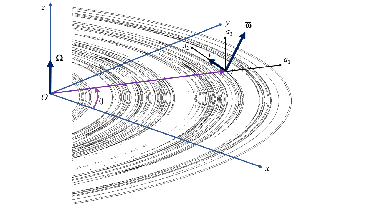
Figure 1: The planar ring of particles, adapted from (Li and Ostoja-Starzewski, 2015, Fig. 5(b)), showing the Saturnian (Cartesian and cylindrical) coordinate systems as well as the orbital frame of reference $\mathbf{(}a_{1},a_{2},a_{3})$ and the body axes $\mathbf{(}x_{1},x_{2},x_{3})$ of a typical particle.

Henceforth, we consider two rings: Euclidean (i.e. non-fractal) and a fractal one; both rings are planar, Fig. 1. Hereinafter the subscript _E denotes any Euclidean object. Next, we must consider the mass of a Euclidean ring (body $B_{\mathbb{E}}$) versus a fractal ring (body $B_{\alpha}$). From a discrete system point of view, the ring is made of $I$ particles $\{i=1,...,I\}$, each with a respective mass $m_{i}$, moment of inertia $\mathbf{j}_{i}$, and positions $\mathbf{x}_{i}$.

The mass of a Euclidean ring $B_{\mathbb{E}}$, with radius $r\in[R_{D},R]$ and thickness $h$ in $z$-direction, is now taken in a continuum sense

$$\begin{array}[]{c}M_{\mathbb{E}}=\sum_{i=1}^{I}m_{i}\rightarrow\int_{B_{\mathbb{E}}}\rho dB_{\mathbb{E}}=h\int_{R_{D}}^{R}\int_{0}^{2\pi}\rho_{\mathbb{E}}hdS_{2}\\ =2\pi h\rho_{\mathbb{E}}\int_{R_{D}}^{R}rdr=\rho_{\mathbb{E}}h\pi\left(R^{2}-R_{D}^{2}\right).\end{array}$$ (1)

In the above we have assumed the mass to be homogeneously distributed throughout the ring with a mass density $\rho_{\mathbb{E}}$. To get quantitative results, one may take: $R=140\times 10^{6}m$ as the outer radius of Saturn’s F ring, $R_{D}=74.5\times 10^{6}m$ as the radius of the (inner) D ring, and the rings’ thickness $h=100m$.

2.2 Mass densities

All the rings constituting the fractal ring $B_{\alpha}$ are embedded in $\mathbb{R}^{3}$, also with radius $r\in[R_{D},R]$ and thickness $h$ in $z$-direction. The parameter $\alpha$ ($<1$) denotes the fractal dimension in the radial direction, i.e. on any ray(any because the ring is axially symmetric about $z$). Thus, the (planar) fractal dimension, such as seen and measured on photographs, is $D=\alpha+1<2$, consistent with the fact that Saturn’s rings are partially plane-filling if interpreted as a planar body. In order to do any analysis involving $B_{\alpha}$, in the vein of Tarasov (2005, 2006), we employ the integration in non-integer dimensional space. That is, we take the infinitesimal element $dB_{\alpha}$ of $B_{\alpha}$ according to (Li and Ostoja-Starzewski, 2013):

$$dB_{\alpha}=h\text{ }dS_{\alpha},\text{ \ \ }dS_{\alpha}=\alpha\left(\frac{r}{R}\right)^{\alpha-1}dS,\text{ \ \ }dS=rdrd\theta.$$ (2)

Now, the mass of a fractal ring is

$$\begin{array}[]{c}M_{\alpha}=\sum_{i=1}^{I}m_{i}\rightarrow\int_{B}\rho_{\alpha}dB_{\alpha}=h\int_{R_{D}}^{R}\int_{0}^{2\pi}\rho_{\alpha}dS_{\alpha}\\ =\displaystyle 2\pi h\rho_{\alpha}\int_{R_{D}}^{R}\alpha\left(\frac{r}{R}\right)^{\alpha-1}rdr=2\pi h\rho_{\alpha}\frac{\alpha}{\alpha+1}\left(R^{2}-\frac{R_{D}^{\alpha+1}}{R^{\alpha-1}}\right),\end{array}$$ (3)

which involves an effective mass density $\rho_{\alpha}$ of a fractal ring. Note that the above correctly reduces to (1) for $\alpha\rightarrow 1$. Since the rings in both interpretations must have the same mass, requiring $M_{\alpha}=M_{\mathbb{E}}$ for any $\alpha$, gives

$$\rho_{\alpha}=\frac{\alpha+1}{2\alpha}\rho_{\mathbb{E}},$$ (4)

which is a decreasing function of $\alpha$ (i.e. we must have $\rho_{\alpha}>\rho_{\mathbb{E}}$ for $\alpha<1$) and which correctly gives $\lim_{\alpha\rightarrow 1}\rho_{\alpha=1}=\rho_{\mathbb{E}}$ for $\alpha=1$, i.e. when the fractal ring becomes non-fractal. Thus, a fractal ring has a higher effective mass density than the homogeneous Euclidean ring of the same overall dimensions.

2.3 Moments of inertia

The moment of inertia of the Euclidean ring ($r\in[0,R]$ and thickness $h$ in $z$-direction), assuming $\rho_{\mathbb{E}}=\mathrm{const}$, is

$$I_{\mathbb{E}}=\frac{1}{2}\pi h\rho_{\mathbb{E}}\left(R^{4}-R_{D}^{4}\right)=\frac{1}{2}M\left(R^{2}+R_{D}^{2}\right),$$ (5)

while the moment of inertia of a fractal ring is

$$\begin{array}[]{c}I_{\alpha}=h\int_{B}\rho_{\alpha}r^{2}dB_{E}=h\int_{R_{D}}^{R}\int_{0}^{2\pi}r^{2}\rho_{\alpha}hdS_{\alpha}\\ \displaystyle 2\pi h\rho_{\alpha}\int_{R_{D}}^{R}r^{2}\alpha\left(\frac{r}{R}\right)^{\alpha-1}rdr=2\pi h\rho_{\alpha}\frac{\alpha}{\alpha+3}\left(R^{4}-\frac{R_{D}^{\alpha+3}}{R^{\alpha-1}}\right).\end{array}$$ (6)

Now, take the limit $\alpha\rightarrow 1$:

$$\lim_{\alpha\rightarrow 1}I_{\alpha}=\frac{1}{2}\pi h\rho_{\mathbb{E}}\left(R^{4}-R_{D}^{4}\right)=I_{\mathbb{E}},$$ (7)

as expected. Note that $I_{\alpha}$ is an increasing function of $\alpha$ (i.e. we must have $I_{\alpha}<I_{\mathbb{E}}$ for $\alpha<1$) and which correctly gives $\lim_{\alpha\rightarrow 1}I_{\alpha}=I_{\mathbb{E}}$ for $\alpha=1$. We also observe from (6) that a fractal ring has a lower moment of inertia than the homogeneous Euclidean ring with the same overall dimensions.

2.4 Energies

Since for an object of mass $m$ on a circular orbit the total energy is $E=-\mu/2r$, the total energy (sum of kinetic and potential) of the Euclidean ring is

$$\begin{array}[]{c}\displaystyle E_{\mathbb{E}}=-\sum_{i=1}^{I}\frac{\mu m_{i}}{2r_{i}}\rightarrow-\int_{B}\frac{\mu\rho_{E}}{2r}\text{ }dB\\ =\displaystyle-\frac{1}{2}h\mu\rho_{\mathbb{E}}\int_{0}^{R}\int_{0}^{2\pi}r^{-1}rdrd\theta=-\pi h\mu\rho_{\mathbb{E}}\left(R-R_{D}\right).\end{array}$$ (8)

On the other hand, the total energy of the fractal ring $B_{\alpha}$ is [again with $dS_{\alpha}=\alpha\left(\frac{r}{R}\right)^{\alpha-1}rdrd\theta$]

$$\begin{array}[]{c}E_{\alpha}=\displaystyle-\sum_{i=1}^{I}\frac{\mu m_{i}}{2r_{i}}\rightarrow-\int_{B}\frac{\mu\rho_{\alpha}}{2r}\text{ }dB=-\int_{R_{D}}^{R}\frac{1}{2}h\mu\rho_{\alpha}\frac{\alpha+1}{2\alpha}r^{-1}dS_{\alpha}\\ =\displaystyle-\int_{R_{D}}^{R}\int_{0}^{2\pi}\frac{1}{2}h\mu\rho_{\alpha}\alpha\frac{\alpha+1}{2\alpha}r^{-1}\left(\frac{r}{R}\right)^{\alpha-1}rdrd\theta=-\pi h\mu\rho_{\alpha}\frac{\alpha+1}{2\alpha}\left(R-R_{D}\right).\end{array}$$ (9)

Now, take the limit $\alpha\rightarrow 1$:

$$\lim_{\alpha\rightarrow 1}E_{\alpha}=\frac{1}{2}\pi h\rho_{\mathbb{E}}\left(R-R_{D}\right)=E_{\mathbb{E}},$$ (10)

as expected.

Comparing $E_{\alpha}$ with $E_{\mathbb{E}}$, gives

$$E_{\alpha}=\frac{\alpha+1}{2\alpha}E_{\mathbb{E}},$$ (11)

which is a decreasing function of $\alpha$. Thus, given the minus sign in (8) and (9), the fractal ring has a lower total energy than the homogeneous Euclidean ring with the same overall dimensions and the same mass. In other words, with reference to question Q1 in the Introduction, the ring having a fractal structure is more likely than that with a non-fractal one.

The foregoing argument extends the approach of Yang (2007), who showed that a Euclidean ring has a lower energy than a Euclidean spherical shell, which in turn is lower than that of a Euclidean ball. Putting all the inequalities together, we have

$$E_{\alpha}\leq E_{\mathbb{E}}\leq E_{\mathrm{shell}}\leq E_{\mathrm{ball}}.$$

2.5 Angular Momenta

For any particle of velocity $v$ on a circular orbit of radius $r$ around a planet:

$$\mu=rv^{2}=r^{3}\Omega^{2}=4\pi^{2}r^{3}/T^{2},$$ (12)

where $\Omega$ is the angular velocity and $T$ is the period. This implies:

$$v=\sqrt{\mu/r}\text{\ \ \ and \ \ }\Omega=\sqrt{\mu/r^{3}}.$$ (13)

For the Euclidean ring ($r\in[0,R]$ and thickness $h$ in $z$-direction), the angular momentum is

$$\begin{array}[]{c}\displaystyle H_{\mathbb{E}}=\sum_{i=1}^{I}m_{i}r_{i}v_{i}\rightarrow h\int_{R_{D}}^{R}\int_{0}^{2\pi}\rho_{\mathbb{E}}rv\text{ }rdrd\theta\\ =\displaystyle h\int_{R_{D}}^{R}\int_{0}^{2\pi}\rho_{\mathbb{E}}r\sqrt{\mu/r}\text{ }rdrd\theta=2\pi h\rho_{\mathbb{E}}\sqrt{\mu}\frac{2}{5}\left(R^{5/2}-R_{D}^{5/2}\right),\end{array}$$ (14)

while for the fractal ring $B_{\alpha}$, the angular momentum is

$$\begin{array}[]{c}H_{\alpha}=\sum_{i=1}^{I}m_{i}r_{i}v_{i}\rightarrow h\int_{0}^{R}\int_{R_{D}}^{2\pi}\rho(r)rv\text{ }dS_{\alpha}=\displaystyle 2\pi h\rho_{\alpha}\int_{R_{D}}^{R}r\sqrt{\frac{\mu}{r}}\alpha\left(\frac{r}{R}\right)^{\alpha-1}\text{ }rdr\\ =\displaystyle 2\pi h\rho_{\alpha}\sqrt{\mu}\frac{\alpha}{\alpha+3/2}R^{1-\alpha}\left(R^{3/2+\alpha}-R_{D}^{3/2+\alpha}\right).\end{array}$$ (15)

This correctly reduces to $H_{\mathbb{E}}$ above for $\alpha\rightarrow 1$.

Comparing $H_{\alpha}$ with $H_{\mathbb{E}}$, shows that $H_{\alpha}$ is an increasing function of $\alpha$ and this correctly gives $\lim_{\alpha\rightarrow 1}H_{\alpha=1}=H_{\mathbb{E}}$, i.e. the fractal ring has a lower angular momentum than the homogeneous Euclidean ring with the same overall dimensions.

At this point, we note that in inelastic collisions the momentum is conserved (just as in elastic collisions), but the kinetic energy is not as it is partially converted to other forms of energy. If this argument is applied to the rings, one may argue that $H_{\alpha}=H_{\mathbb{E}}$ should hold for any $\alpha$, which can be satisfied by accounting for the angular momentum of particles due to rotation about their own axes . Thus, instead of (13), writing $j_{i}$ for the moment of inertia of the particle $i$, we have the contribution of the angular momentum of that rotation in terms of the Euler angle $\phi$ about the $a_{3}$ axis:

$$H_{\mathbb{E}}=\sum_{i=1}^{I}m_{i}r_{i}v_{i}+\sum_{i\in I}j_{i}\omega_{zi}\rightarrow h\int_{R_{D}}^{R}\int_{0}^{2\pi}\rho_{\mathbb{E}}rv\text{ }rdrd\theta+h\int_{R_{D}}^{R}\int_{0}^{2\pi}j\phi\text{ }rdrd\theta.$$ (16)

The first integral can be calculated as before, while in the second one we could assume $j=const$ although this would still leave the microrotation $\omega_{z}$ as an unknown function of $r$. Turning to the fractal ring we also have two terms

$$H_{\alpha}=\sum_{i=1}^{I}m_{i}r_{i}v_{i}+\sum_{i\in I}j_{i}\omega_{zi}\rightarrow h\int_{R_{D}}^{R}\int_{0}^{2\pi}\rho_{E}rv\text{ }dS_{\alpha}+h\int_{R_{D}}^{R}\int_{0}^{2\pi}j\phi\text{ }dS_{\alpha},$$ (17)

showing that the statistics $\omega_{z}\left(r\right)$ needs to be determined. At this point we turn to the question Q2.

3 A stochastic model of kinematics

First, we consider the particles in Saturn’s rings at a time moment $0$.

Introduce a spherical coordinate system $(r,\varphi,\theta)$ with origin $O$ in the centre of Saturn such that the plane of Saturn’s rings corresponds to the polar angle’s value $\theta=\pi/2$. Let $\overline{\bm{\omega}}(r,\varphi)\in\mathbb{R}^{3}$ be the angular velocity vector of a rotating particle located at $(r,\varphi)$. We assume that $\overline{\bm{\omega}}(r,\varphi)$ is a single realisation of a random field.

To explain the exact meaning of this construction, we proceed as follows. Let $(x,y,z)$ be a Cartesian coordinate system with origin in the centre of Saturn such that the plane of Saturn’s rings corresponds to the $xy$-plane, Fig. 1. Let $O(2)$ be the group of real orthogonal $2\times 2$ matrices, and let $SO(2)$ be its subgroup consisting of matrices with determinant equal to $1$. Put $G=O(2)\times SO(2)$, $K=O(2)$. The homogeneous space $C=G/K=SO(2)$ can be identified with a circle, the trajectory of a particle inside rings.

Consider the real orthogonal representation $U$ of the group $O(2)$ in $\mathbb{R}^{3}$ defined by

$$g=\begin{pmatrix}g_{11}&g_{12}\\ g_{21}&g_{22}\end{pmatrix}\mapsto U(g)=\begin{pmatrix}g_{11}&g_{12}&0\\ g_{21}&g_{22}&0\\ 0&0&\det g\end{pmatrix}.$$ (18)

Introduce an equivalence relation in the Cartesian product $G\times\mathbb{R}^{3}$: two elements $(g_{1},\mathbf{x}_{1})$ and $(g_{2},\mathbf{x}_{2})$ are equivalent if and only if there exists an element $g\in O(2)$ such that $(g_{2},\mathbf{x}_{2})=(g_{1}g,U(g^{-1})\mathbf{x}_{1})$. The projection map maps an element $(g,\mathbf{x})\in G\times\mathbb{R}^{3}$ to its equivalence class and defines the quotient topology on the set $E_{U}$ of equivalence classes. Another projection map,

$$\pi\colon E_{U}\to C,\qquad\pi(g,\mathbf{x})=gK,$$

determines a vector bundle $\xi=(E_{U},\pi,C)$.

The topological space $R=\mathbb{R}^{2}\setminus\{\mathbf{0}\}$ is the union of circles $C_{r}$ of radiuses $r>0$. Every circle determines the vector bundle $\xi_{r}=(E_{Ur},\pi_{r},C_{r})$. Consider the vector bundle $\eta=(E,\pi,R)$, where $E$ is the union of all $E_{Ur}$, and the restriction of the projection map $\pi$ to $E_{Ur}$ is equal to $\pi_{r}$. The random field $\overline{\bm{\omega}}(r,\varphi)$ is a random section of the above bundle, that is, $\overline{\bm{\omega}}(r,\varphi)\in\pi^{-1}(r,\varphi)=\mathbb{R}^{3}$. In what follow we assume that the random field $\overline{\bm{\omega}}(r,\varphi)$ is second-order, i.e., $\mathsf{E}[\|\overline{\bm{\omega}}(r,\varphi)\|^{2}]<\infty$ for all $(r,\varphi)\in R$.

There are at least three different (but most probably equivalent) approaches to the construction of random sections of vector bundles, the first by Geller and Marinucci (2010), the second by Malyarenko (2011, 2013), and the third by Baldi and Rossi (2014). In what follows, we will use the second named approach. It is based on the following fact: the vector bundle $\eta=(E,\pi,R)$ is homogeneous or equivariant. In other words, the action of the group $O(2)$ on the bundle base $R$ induces the action of $O(2)$ on the total space $E$ by $(g_{0},\mathbf{x})\mapsto(gg_{0},\mathbf{x})$. This action identifies the spaces $\pi^{-1}(r_{0},\varphi)$ for all $\varphi\in[0,2\pi)$, while the action of the multiplicative group $\mathbb{R}^{+}$ on R, $\lambda(r,\varphi)=(\lambda r,\varphi)$, $\lambda>0$, identifies the spaces $\pi^{-1}(r,\varphi_{0})$ for all $r>0$. We suppose that the random field $\overline{\bm{\omega}}(r,\varphi)$ is mean-square continuous, i.e.,

$$\lim_{\|\mathbf{x}-\mathbf{x}_{0}\|\to 0}\mathsf{E}[\|\overline{\bm{\omega}}(\mathbf{x})-\overline{\bm{\omega}}(\mathbf{x}_{0}))\|^{2}]=0$$

for all $\mathbf{x}_{0}\in R$.

Let $\langle\overline{\bm{\omega}}(\mathbf{x})\rangle=\mathsf{E}[\overline{\bm{\omega}}(\mathbf{x})]$ be the one-point correlation vector of the random field $\overline{\bm{\omega}}(\mathbf{x})$. On the one hand, under rotation and/or reflection $g\in O(2)$ the point $\mathbf{x}$ becomes the point $g\mathbf{x}$. Evidently, the axial vector $\overline{\bm{\omega}}(\mathbf{x})$ transforms according to the representation (18) and becomes $U(g)\overline{\bm{\omega}}(g\mathbf{x})$. The one-point correlation vector of the so transformed random field remains the same, i.e.,

$$\langle\overline{\bm{\omega}}(g\mathbf{x})\rangle=U(g)\langle\overline{\bm{\omega}}(\mathbf{x})\rangle.$$

On the other hand, the one-point correlation vector of the random field $\overline{\bm{\omega}}(r,\varphi)$ should be independent upon an arbitrary choice of the $x$- and $y$-axes of the Cartesian coordinate systems, i.e., it should not depend on $\varphi$. Then we have

$$\langle\overline{\bm{\omega}}(\mathbf{x})\rangle=U(g)\langle\overline{\bm{\omega}}(\mathbf{x})\rangle$$

for all $g\in O(2)$, i.e., $\langle\overline{\bm{\omega}}(\mathbf{x})\rangle$ belongs to a subspace of $\mathbb{R}^{3}$ where a trivial component of $U$ acts. Then we obtain $\langle\overline{\bm{\omega}}(\mathbf{x})\rangle=\mathbf{0}$, because $U$ does not contain trivial components.

Similarly, let $\langle\overline{\bm{\omega}}(\mathbf{x}),\overline{\bm{\omega}}(\mathbf{y})\rangle=\mathsf{E}[\overline{\bm{\omega}}(\mathbf{x})\otimes\overline{\bm{\omega}}(\mathbf{y})]$ be the two-point correlation tensor of the random field $\overline{\bm{\omega}}(\mathbf{x})$. Under the action of $O(2)$ we should have

$$\langle\overline{\bm{\omega}}(g\mathbf{x}),\overline{\bm{\omega}}(g\mathbf{y})\rangle=(U\otimes U)(g)\langle\overline{\bm{\omega}}(\mathbf{x}),\overline{\bm{\omega}}(\mathbf{y})\rangle.$$

In other words, the random field $\overline{\bm{\omega}}(\mathbf{x})$ is wide-sense isotropic with respect to the group $O(2)$ and its representation $U$.

Consider the restriction of the field $\overline{\bm{\omega}}(\mathbf{x})$ to a circle $C_{r}$, $r>0$. The spectral expansion of the field $\{\,\overline{\bm{\omega}}(r,\varphi)\colon\varphi\in C_{r}\,\}$ can be calculated using Malyarenko (2011, Theorem 2) or Malyarenko (2013, Theorem 2.28).

The representation $U$ is the direct sum of the two irreducible representations $\lambda_{-}(g)=\det g$ and $\lambda_{1}(g)=g$. The vector bundle $\eta$ is the direct sum of the vector bundles $\eta_{-}$ and $\eta_{1}$, where the bundle $\eta_{-}$ (resp. $\eta_{1}$) is generated by the representation $\lambda_{-}$ (resp. $\lambda_{1}$). Let $\mu_{0}$ be the trivial representation of the group $SO(2)$, and let $\mu_{k}$ be the representation

$$\mu_{k}(\varphi)=\begin{pmatrix}\cos(k\varphi)&\sin(k\varphi)\\ -\sin(k\varphi)&\cos(k\varphi)\end{pmatrix}.$$

The representations $\lambda_{-}\otimes\mu_{k}$, $k\geq 0$ are all irreducible orthogonal representations of the group $G=O(2)\times SO(2)$ that contain $\lambda_{-}$ after restriction to $O(2)$. The representations $\lambda_{1}\otimes\mu_{k}$, $k\geq 0$ are all irreducible orthogonal representations of the group $G=O(2)\times SO(2)$ that contain $\lambda_{1}$ after restriction to $O(2)$. The matrix entries of $\mu_{0}$ and of the second column of $\mu_{k}$ form an orthogonal basis in the Hilbert space $L^{2}(SO(2),\mathrm{d}\varphi)$. Their multiples

$$e_{k}(\varphi)=\begin{cases}\frac{1}{\sqrt{2\pi}},&\mbox{if }k=0,\\ \frac{1}{\sqrt{\pi}}\cos(k\varphi),&\mbox{if }k\leq-1\\ \frac{1}{\sqrt{\pi}}\sin(k\varphi),&\mbox{if }k\geq 1\end{cases}$$

form an orthonormal basis of the above space. Then we have

$$\overline{\bm{\omega}}(r,\varphi)=\sum_{k=-\infty}^{\infty}e_{k}(\varphi)\mathbf{Z}^{k}(r),$$ (19)

where $\{\,\mathbf{Z}^{k}(r)\colon k\in\mathbb{Z}\,\}$ is a sequence of centred stochastic processes with

$$\mathsf{E}[\mathbf{Z}^{k}(r)\otimes\mathbf{Z}^{l}(r)] =\delta_{kl}B^{(k)}(r),$$

$$\sum_{k\in\mathbb{Z}}\operatorname{tr}(B^{(k)}(r)) <\infty.$$

It follows that

$$\mathbf{Z}^{k}(r)=\int_{0}^{2\pi}\overline{\bm{\omega}}(r,\varphi)e_{k}(\varphi)\,\mathrm{d}\varphi.$$

Then we have

$$\mathsf{E}[\mathbf{Z}^{k}(r)\otimes\mathbf{Z}^{l}(s)]=\int_{0}^{2\pi}\int_{0}^{2\pi}\mathsf{E}[\overline{\bm{\omega}}(r,\varphi_{1})\otimes\overline{\bm{\omega}}(s,\varphi_{2})]e_{k}(\varphi_{1})\,\mathrm{d}\varphi_{1}e_{l}(\varphi_{2})\,\mathrm{d}\varphi_{2}.$$ (20)

The field is isotropic and mean-square continuous, therefore

$$\mathsf{E}[\overline{\bm{\omega}}(r,\varphi_{1})\otimes\overline{\bm{\omega}}(s,\varphi_{2})]=B(r,s,\cos(\varphi_{1}-\varphi_{2}))$$

is a continuous function. Note that $e_{k}(\varphi)$ are spherical harmonics of degree $|k|$. Denote by $\mathbf{x\cdot y}$ the standard inner product in the space $\mathbb{R}^{d}$, and by $\mathrm{d}\omega(\mathbf{y})$ the Lebesgue measure on the unit sphere $S^{d-1}=\{\,\mathbf{x}\in\mathbb{R}^{d}\colon\|\mathbf{x}\|=1\,\}$. Then

$$\int_{S^{d-1}}\,\mathrm{d}\omega(\mathbf{x})=\omega_{d}=\frac{2\pi^{d/2}}{\Gamma(d/2)},$$

where $\Gamma$ is the Gamma function.

Now we use the Funk–Hecke theorem, see Andrews et al. (1999). For any continuous function $f$ on the interval $[-1,1]$ and for any spherical harmonic $S_{k}(\mathbf{y})$ of degree $k$ we have

$$\int_{S^{d-1}}f(\mathbf{x\cdot y})S_{k}(\mathbf{x})\,\mathrm{d}\omega(\mathbf{x})=\lambda_{k}S_{k}(\mathbf{y}),$$

where

$$\lambda_{k}=\omega_{d-1}\int_{-1}^{1}f(u)\frac{C^{(n-2)/2}_{k}(u)}{C^{(n-2)/2}_{k}(1)}(1-u^{2})^{(n-3)/2}\,\mathrm{d}u,$$

$d\geq 3$, and $C^{(n-2)/2}_{k}(u)$ are Gegenbauer polynomials. To see how this theorem looks like when $d=2$, we perform a limit transition as $n\downarrow 2$. By Andrews et al. (1999, Equation 6.4.13’),

$$\lim_{\lambda\to 0}\frac{C^{\lambda}_{k}(u)}{C^{\lambda}_{k}(1)}=T_{k}(u),$$

where $T_{k}(u)$ are Chebyshev polynomials of the first kind. We have $\omega_{1}=2$, $\mathbf{x\cdot y}$ becomes $\cos(\varphi_{1}-\varphi_{2})$, and $\mathrm{d}\omega(\mathbf{x})$ becomes $\mathrm{d}\varphi_{1}$. We obtain

$$\int_{0}^{2\pi}B(r,s,\cos(\varphi_{1}-\varphi_{2}))e_{k}(\varphi_{1})\,\mathrm{d}\varphi_{1}=B^{(k)}(r,s)e_{k}(\varphi_{2}),$$

where

$$B^{(k)}(r,s)=2\int_{-1}^{1}B(r,s,u)T_{|k|}(u)(1-u^{2})^{-1/2}\,\mathrm{d}u,$$

Equation (20) becomes

$$\mathsf{E}[\mathbf{Z}^{k}(r)\otimes\mathbf{Z}^{l}(s)]=\int_{0}^{2\pi}B^{(k)}(r,s)e_{k}(\varphi_{2})e_{l}(\varphi_{2})\,\mathrm{d}\varphi_{2}=\delta_{kl}B^{(k)}(r,s).$$

In particular, if $k\neq l$, then the processes $\mathbf{Z}^{k}(r)$ and $\mathbf{Z}^{l}(r)$ are uncorrelated.

Calculate the two-point correlation tensor of the random field $\overline{\bm{\omega}}(r,\varphi)$. We have

$$\mathsf{E}[\overline{\bm{\omega}}(r,\varphi_{1})\otimes\overline{\bm{\omega}}(s,\varphi_{2})] =\sum_{k=-\infty}^{\infty}e_{k}(\varphi_{1})e_{k}(\varphi_{2})B^{(k)}(r,s)$$ (21)

$$=\frac{1}{2\pi}B^{(0)}(r,s)+\frac{1}{\pi}\sum_{k=1}^{\infty}\cos(k(\varphi_{1}-\varphi_{2}))B^{(k)}(r,s).$$

Now we add a time coordinate, $t$, to our considerations. A particle located at $(r,\varphi)$ at time moment $t$, was located at $(r,\varphi-\sqrt{GM}t/r^{3/2})$ at time moment $0$. It follows that

$$\overline{\bm{\omega}}(t,r,\varphi)=\overline{\bm{\omega}}\left(r,\varphi-\frac{\sqrt{GM}t}{r^{3/2}}\right),$$

where $G$ is Newton’s gravitational constant and $M$ is the mass of Saturn. Equation (19) gives

$$\overline{\bm{\omega}}(t,r,\varphi)=\sum_{k=-\infty}^{\infty}e_{k}\left(\varphi-\frac{\sqrt{GM}t}{r^{3/2}}\right)\mathbf{Z}^{k}(r),$$ (22)

while Equation (21) gives

$$\mathsf{E}[\overline{\bm{\omega}}(t_{1},r,\varphi_{1})\otimes\overline{\bm{\omega}}(t_{2},s,\varphi_{2})] =\frac{1}{2\pi}B^{(0)}(r,s)$$

$$\quad+\frac{1}{\pi}\sum_{k=1}^{\infty}\cos\left(k\left(\varphi_{1}-\varphi_{2}-\frac{\sqrt{GM}(t_{1}-t_{2})}{r^{3/2}}\right)\right)B^{(k)}(r,s).$$

Conversely, let $\{\,B^{(k)}(r,s)\colon k\geq 0\,\}$ be a sequence of continuous positive-definite matrix-valued functions with

$$\sum_{k=0}^{\infty}\operatorname{tr}(B^{(k)}(r,r))<\infty,$$ (23)

and let $\{\,\mathbf{Z}_{k}(r)\colon k\in\mathbb{Z}\,\}$ be a sequence of uncorrelated centred stochastic processes with

$$\mathsf{E}[\mathbf{Z}^{k}(r)\otimes\mathbf{Z}^{l}(s)]=\delta_{kl}B^{(|k|)}(r,s).$$

The random field (22) may describe rotating particles inside Saturn’s rings, if all the functions $B^{(k)}(r,s)$ are equal to $0$ outside the rectangle $[R_{0},R_{1}]^{2}$, where $R_{0}$ (resp. $R_{1}$) is the inner (resp. outer) radius of Saturn’s rings.

To make our model more realistic, we assume that all the functions $B^{(k)}(r,s)$ are equal to $0$ outside the Cartesian square $F^{2}$, where $F$ is a fat fractal subset of the interval $[R_{0},R_{1}]$, see Umberger and Farmer (1985). Mandelbrot (1982) calls these sets dusts of positive measure. Such a set has a positive Lebesgue measure, its Hausdorff dimension is equal to $1$, but the Hausdorff dimension of its boundary is not an integer number.

A classical example of a fat fractal is a fat Cantor set. In contrast to the ordinary Cantor set, where we delete the middle one-third of each interval at each step, this time we delete the middle $3^{-n}$th part of each interval at the $n$th step.

To construct an example, consider an arbitrary sequence of continuous positive-definite matrix-valued functions $\{\,B^{(k)}(r,s)\colon k\geq 0\,\}$ satisfying (23) of the following form:

$$B^{(k)}(r,s)=\sum_{i\in I_{k}}\mathbf{f}_{ik}(r)\mathbf{f}^{\top}_{ik}(s),$$

where $\mathbf{f}_{ik}(r)\colon[R_{0},R_{1}]\to\mathbb{R}^{3}$ are continuous functions, satisfying the following condition: for each $r\in[R_{0},R_{1}]$ the set $I_{kr}=\{\,i\in I_{k}\colon f_{i}(r)\neq 0\,\}$ is as most countable and the series

$$\sum_{i\in I_{kr}}\|\mathbf{f}_{i}(r)\|^{2}$$

converges. The so defined function is obviously positive-definite. Put

$$\tilde{B}^{(k)}(r,s)=\sum_{i\in I_{k}}\tilde{\mathbf{f}}_{ik}(r)\tilde{\mathbf{f}}^{\top}_{ik}(s),\qquad r,s\in F.$$

The functions $\tilde{B}^{(k)}(r,s)$ are the restrictions of positive-definite functions $B^{(k)}(r,s)$ to $F^{2}$ and are positive-definite themselves. Consider the centred stochastic process $\{\,\tilde{\mathbf{Z}}^{k}(r)\colon r\in F\,\}$ with

$$\mathsf{E}[\tilde{\mathbf{Z}}^{k}(r)\otimes\tilde{\mathbf{Z}}^{l}(s)]=\delta_{kl}\tilde{B}^{(|k|)}(r,s),\qquad r,s\in F.$$

Condition (23) guarantees the mean-square convergence of the series

$$\overline{\bm{\omega}}(t,r,\varphi)=\sum_{k=-\infty}^{\infty}e_{k}\left(\varphi-\frac{\sqrt{GM}t}{r^{3/2}}\right)\tilde{\mathbf{Z}}^{k}(r)$$

for all $t\geq 0$, $r\in F$, and $\varphi\in[0,2\pi]$.

4 Closure

This paper reports an investigation of the fractal character of Saturnian rings. First, working with the calculus in a non-integer dimensional space, by energy arguments, we infer that the fractally structured ring is more likely than a non-fractal one. Next, we develop a kinematics model in which angular velocities of particles form a random field.

References

- Andrews et al. (1999) G. E. Andrews, R. Askey, and R. Roy. Special functions, volume 71 of Encyclopedia of Mathematics and its Applications. Cambridge University Press, Cambridge, 1999.
- Avron and Simon (1981) J. E. Avron and B. Simon. Almost periodic Hill’s equation and the rings of Saturn. Phys. Rev. Lett., 46(17):1166–1168, 1981.
- Baldi and Rossi (2014) P. Baldi and M. Rossi. Representation of Gaussian isotropic spin random fields. Stochastic Process. Appl., 124(5):1910–1941, 2014.
- Geller and Marinucci (2010) D. Geller and D. Marinucci. Spin wavelets on the sphere. J. Fourier Anal. Appl., 16(6):840–884, 2010.
- Li and Ostoja-Starzewski (2013) J. Li and M. Ostoja-Starzewski. Comment on “Hydrodynamics of fractal continuum flow” and “Map of fluid flow in fractal porous medium into fractal continuum flow”. Phys. Rev. E, 88:057001, Nov 2013.
- Li and Ostoja-Starzewski (2015) J. Li and M. Ostoja-Starzewski. Edges of Saturn’s rings are fractal. SpringerPlus, 4(1):158, 2015.
- Malyarenko (2011) A. Malyarenko. Invariant random fields in vector bundles and application to cosmology. Ann. Inst. Henri Poincaré Probab. Stat., 47(4):1068–1095, 2011.
- Malyarenko (2013) A. Malyarenko. Invariant random fields on spaces with a group action. Probability and its Applications (New York). Springer, Heidelberg, 2013.
- Mandelbrot (1982) B. B. Mandelbrot. The fractal geometry of nature. Schriftenreihe für den Referenten. [Series for the Referee]. W. H. Freeman and Co., San Francisco, Calif., 1982.
- Tarasov (2005) V. E. Tarasov. Dynamics of fractal solids. Int. J. Mod. Phys. B, 19(27):4103–4114, 2005.
- Tarasov (2006) V. E. Tarasov. Gravitational field of fractal distribution of particles. Celestial Mech. Dynam. Astronom., 94(1):1–15, 2006.
- Umberger and Farmer (1985) D. K. Umberger and J. D. Farmer. Fat fractals on the energy surface. Phys. Rev. Lett., 55:661–664, Aug 1985.
- Yang (2007) X. Yang. Applied Engineering Mathematics. Cambridge International Science Publishing, 2007.