Improper Signaling in Two-Path Relay Channels

Abstract

Inter-relay interference (IRI) challenges the operation of two-path relaying systems. Furthermore, the unavailability of the channel state information (CSI) at the source and the limited detection capabilities at the relays prevent neither eliminating the interference nor adopting joint detection at the relays nodes. Improper signaling is a powerful signaling scheme that has the capability to reduce the interference impact at the receiver side and improves the achievable rate performance. Therefore, improper signaling is adopted at both relays, which have access to the global CSI. Then, improper signal characteristics are designed to maximize the total end-to-end achievable rate at the relays. To this end, both the power and the circularity coefficient, a measure of the impropriety degree of the signal, are optimized at the relays. Although the optimization problem is not convex, optimal power allocation for both relays for a fixed circularity coefficient is obtained. Moreover, the circularity coefficient is tuned to maximize the rate for a given power allocation. Finally, a joint solution of the optimization problem is proposed using a coordinate descent method based on alternate optimization. The simulation results show that employing improper signaling improves the achievable rate at medium and high IRI.

I Introduction

Next generation wireless communication adopts technologies that extends the network coverage and improve the data rate. One of the candidate technologies is full-duplex relaying that targets to double the spectral efficiency. On the other hand, cooperative communication is an interesting technology to improve the data rate and extend the communication range. Full-duplex relaying is employed to extend the network coverage while improving the link quality. Despite of the promising performance that full-duplex can achieve, replacing all half-duplex nodes by full-duplex ones is not possible to be done immediately. During the roll-out phase, half-duplex nodes are used to support full-duplex services. Two path relaying, which is also known as, alternate relaying, is a distributed realization of full-duplex relaying. Full-duplex relaying suffers from self-interference, whereas the two-path relaying suffers from inter-relay interference (IRI). Therefore, different interference mitigation techniques need to be adopted to relief the effect of the interference [1].

Improper signaling is used to mitigate the interference impact on communication systems. It is an asymmetric Gaussian signaling scheme that assumes unequal power of the real and imaginary components and/or dependent real and imaginary components. It is used in underlay cognitive radio [2, 3, 4, 5, 6], overlay cognitive radio [7], full-duplex relaying [8], Z-interference channel [9, 10] and asymmetric hardware distortions [11]. Recently, we considered the two-path relaying network and showed that improper signaling can be advantageous over proper signaling to mitigate the IRI [12, 13]. Specifically, in [12], improper signaling is adopted in two-path relaying system, where only the same circularity coefficient, a measure of the degree of impropriety of the signal, for both relays is optimized to mitigate the interference while the relays use their maximum power. On the other hand, in [13], we considered the same problem but with different circularity coefficients at the relays. Moreover, we considered asymmetric time allocation for the two transmission phases while the relays use their maximum power.

In this paper, we take the problem in [12] further and optimize both the relay power and circularity coefficient, which measures the degree of impropriety of the transmit signal, to maximize the end-to-end achievable rate of the two-path relaying system. First, we consider proper signaling and introduce optimal relays power allocation for the system. In the case of using improper signaling, we allocate the relays power with a fixed circularity coefficient. Moreover, we tune the circularity coefficient while fixing the transmit power. Then, we jointly optimize the relays power and circularity coefficient via a coordinate descend based method by iterating between the optimal solutions of the individual problems till a convergence obtained. Finally, we investigate through numerical results the merits that can be reaped if the relays use improper signals using different strategies.

II System Model

We consider here an alternate two-path relaying network consisting of one source node, $S$, two half-duplex relay nodes, $R_{1}$ and $R_{2}$, and one destination node, $D$, as shown in Fig. 1. We adopt decode-and-forward protocol at both relays. Moreover, the relays transmit and receive in turn, i.e., in one time slot one relay receives and the other relay transmits, and in the next time slot the other way around. Let $h_{i}$ and $g_{i}$, $i\in\{1,2\}$, denote the channel between $S$ and $R_{i}$ and the channel between $R_{i}$ and $D$, respectively. We assume channel reciprocity for the inter-relay channel which is denoted by $f$. Moreover, let us assume that the source transmit power is $p_{\rm{s}}$, the relay transmit power is $p_{\rm{r}}$, and the noise variance at each receiving node is $\sigma_{\rm{n}}^{2}$. The transmit powers are limited to a power budget of $p_{\rm{max}}$. First, we give the following definitions of improper random variables (RV).

Definition 1.

[14] The complementary (pseudo-) variance of a zero mean complex random variable $x$ is defined as $\tilde{\sigma}_{x}^{2}=E\{x^{2}\}$, where $\mathbb{E}\{.\}$ denotes the expectation operator. If $\tilde{\sigma}_{x}^{2}=0$, then $x$ is called proper signal, otherwise it is called improper.

Definition 2.

[2] The circularity coefficient of the signal $x$ is a measure of its impropriety degree and is defined as $\mathcal{C}_{x}={|\tilde{\sigma}_{x}^{2}|}/{\sigma_{x}^{2}}$, where ${\sigma}_{x}^{2}=E\{|x|^{2}\}$ is the conventional variance and $|.|$ is the absolute value operation. The circularity coefficient satisfies $0\leq\mathcal{C}_{x}\leq 1$. In particular, $\mathcal{C}_{x}=0$ and $\mathcal{C}_{x}=1$ correspond to proper and maximally improper signals, respectively .

We assume that no channel state information is available at $S$ which necessitates the use of proper signaling at $S$ and also makes dirty paper coding of no benefit to fully cancel the IRI. Also, we assume that no direct link is available between $S$ and $D$. For simplicity and tractability, we consider a yet illustrative scenario by assuming equal power and same circularity coefficient for the relays which may not be optimal. However, as it will be shown in the simulation results, though these sub-optimal assumptions, improper signals show a significantly better performance than proper signaling. Furthermore, we expect even better performance if we increase the degrees of freedom by letting different power and circularity coefficient at the relays. Also, we assume the receivers use the simple practical decoding techniques by treating the interference as a Gaussian noise.

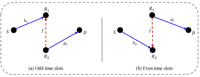
Figure 1: Two-Path Relay Channel. The blue solid lines represent the signal links and the red dashed lines represent the IRI.

During time slot $k$, the signal received at $R_{i}$ with $i=2-\mod(k,2)$ is given by

$$y_{i}[k]=\sqrt{p_{s}}h_{i}[k]s[k]+\sqrt{p_{r}}f[k]x_{j}[k]+n_{i}[k],$$ (1)

where $s[k]$ is the transmit proper signal by $S$ in time slot $k$ and $n_{i}[k]$ is the additive noise at $R_{i}$ with variance $\sigma_{\rm{n}}^{2}$. $x_{j}[k]$ is the improper signal, with circularity coefficient $\mathcal{C}_{x}$, transmitted by $R_{j}$ with $j=1+\mod(k,2)$. The received signal at $D$ from $R_{i}$ in time slot $k+1$ is given by

$$y_{D}[k+1]=\sqrt{p_{r}}g_{i}[k+1]x_{i}[k+1]+n[k+1],$$ (2)

where $n[k+1]$ is the additive noise at $D$. In the following, we assume the channels to be quasi-static block flat fading channels and therefore we drop the time index $k$ for notational convenience. The additive noise at the receivers is modeled as a white, zero-mean, circularly symmetric, complex Gaussian with variance $\sigma_{{n}}^{2}$.

The alternating two-path relaying system mimics a full-duplex system by transferring the data through two Z-interference channels, where two transmitters ($S$ and $R_{i}$) are sending messages each intended for one of the two receivers ($R_{j}$ and $D$) as shown in Fig. 1. Hence, as a result of using improper signals at $R_{j}$ and proper signals at $S$ while treating the interference as a Gaussian noise, the achievable rate of the first hop of the $i$th path ($S-R_{i}$) can be expressed after some simplification steps as [15]

$${\mathcal{R}_{i,1}}\left({{p_{\rm{r}}},{{\cal C}_{x}}}\right)={\log_{2}}\left({1+\frac{{{p_{\rm{s}}}{{\left|{{h_{i}}}\right|}^{2}}}}{{{p_{\rm{r}}}{{\left|f\right|}^{2}}+\sigma_{n}^{2}}}}\right)+\frac{1}{2}{\log_{2}}\left({\frac{{1-{\cal C}_{{{{y}}_{i}}}^{2}}}{{1-{\cal C}_{{\cal{I}}_{i}}^{2}}}}\right),$$ (3)

where ${\cal C}_{{{{y}}_{i}}}$ and ${\cal C}_{{\cal I}_{i}}$ are the circularity coefficients of the received and interference-plus-noise signals at $R_{i}$, respectively, which can be calculated as

$${{\cal C}_{{{{y}}_{i}}}}=\frac{{{p_{\rm{r}}}{{\left|f\right|}^{2}}{{\cal C}_{x}}}}{{{p_{\rm{s}}}{{\left|{{h_{i}}}\right|}^{2}}+{p_{\rm{r}}}{{\left|f\right|}^{2}}+\sigma_{n}^{2}}},\;\;{{\cal C}_{{\cal I}_{i}}}=\frac{{{p_{\rm{r}}}{{\left|f\right|}^{2}}{{\cal C}_{x}}}}{{{p_{\rm{r}}}{{\left|f\right|}^{2}}+\sigma_{n}^{2}}}.$$ (4)

Hence, (3) can be simplified to

$${\mathcal{R}_{i,1}}\left({{p_{\rm{r}}},{{\cal C}_{x}}}\right) =\frac{1}{2}\times$$

$${\log_{2}}\left(1+\frac{{2{p_{\rm{s}}}{{\left|{{h_{i}}}\right|}^{2}}\left({{p_{\rm{r}}}{{\left|f\right|}^{2}}+\sigma_{n}^{2}}\right)+p_{\rm{s}}^{2}{{\left|{{h_{i}}}\right|}^{4}}}}{{\left({1-{\cal C}_{x}^{2}}\right)p_{\rm{r}}^{2}{{\left|f\right|}^{4}}+2{p_{\rm{r}}}{{\left|f\right|}^{2}}\sigma_{n}^{2}+\sigma_{n}^{4}}}\right).$$ (5)

Similarly, the achievable rate of the second hop of the $i$th path can be obtained from (2) as

$${\mathcal{R}_{i,2}}\left({{{p_{\rm{r}},\cal C}_{x}}}\right)={\log_{2}}\left({1+\frac{{{p_{\rm{r}}}{{\left|{{g_{i}}}\right|}^{2}}}}{{\sigma_{n}^{2}}}}\right)+\frac{1}{2}{\log_{2}}\left({\frac{{1-{\cal C}_{{y_{{D}}}}^{2}}}{{1-{\cal C}_{{{\cal I}_{{D}}}}^{2}}}}\right),$$ (6)

where ${\cal C}_{{{{y}}_{D}}}$ and ${\cal C}_{{\cal I}_{D}}$ are the circularity coefficients of the received and interference-plus-noise signals at $D$, respectively, which can be computed as

$${{\cal C}_{{y_{{D}}}}}=\frac{{{p_{\rm{r}}}{{\left|{{g_{i}}}\right|}^{2}}{{\cal C}_{x}}}}{{{p_{\rm{r}}}{{\left|{{g_{i}}}\right|}^{2}}+\sigma_{n}^{2}}},\quad{{\cal C}_{{{\cal I}_{{D}}}}}=0.$$ (7)

Then, (6) reduces to

$${\mathcal{R}_{i,2}}\left({{p_{\rm{r}}},{{\cal C}_{x}}}\right)=\frac{1}{2}{\log_{2}}\left({1+\frac{{2{p_{\rm{r}}}{{\left|{{g_{i}}}\right|}^{2}}}}{{\sigma_{n}^{2}}}+\frac{{p_{\rm{r}}^{2}{{\left|{{g_{i}}}\right|}^{4}}\left({1-{\cal C}_{x}^{2}}\right)}}{{\sigma_{n}^{4}}}}\right).$$ (8)

Hence, the end-to-end achievable rate of the $i$th path can be calculated from

$${\mathcal{R}_{{{}_{i}}}}\left({{p_{\rm{r}}},{{\cal C}_{x}}}\right)=\min\Big{\{}{{\mathcal{R}_{i,1}}\left({{p_{\rm{r}}},{{\cal C}_{x}}}\right),{\mathcal{R}_{i,2}}\left({{p_{\rm{r}}},{{\cal C}_{x}}}\right)}\Big{\}}.$$ (9)

Accordingly, the overall end-to-end achievable rate of the two-path relaying system, for sufficiently large number of time slots, is expressed as the arithmetic mean of ${{\mathcal{R}_{{{}_{i}}}}\left({{p_{\rm{r}}},{{\cal C}_{x}}}\right)}$

$${\mathcal{R}_{{\rm{T}}}}\left({{p_{\rm{r}}},{{\cal C}_{x}}}\right)=\frac{1}{2}\sum\limits_{i=1}^{2}{{\mathcal{R}_{{{}_{i}}}}\left({{p_{\rm{r}}},{{\cal C}_{x}}}\right)}.$$ (10)

Remark 1.

One can notice that if $\mathcal{C}_{x}=0$ in (10), we obtain the conventional expression for the total achievable rate of the two-path relaying system under the use of proper signals as

$${\mathcal{R}_{{\rm{T}}}}\left({{p_{\rm{r}}},0}\right)=\frac{1}{2}\sum\limits_{i=1}^{2}{{\mathcal{R}_{{{}_{i}}}}\left({{p_{\rm{r}}},0}\right)}=\frac{1}{2}\times$$

$$\sum\limits_{i=1}^{2}\min\Bigg{\{}{{\log}_{2}}\left({1+\frac{{{p_{\rm{s}}}{{\left|{{h_{i}}}\right|}^{2}}}}{{\sigma_{n}^{2}+{p_{\rm{r}}}{{\left|f\right|}^{2}}}}}\right),{{\log}_{2}}\left({1+\frac{{{p_{\rm{r}}}{{\left|{{g_{i}}}\right|}^{2}}}}{{\sigma_{n}^{2}}}}\right)\Bigg{\}}.$$ (11)

III Improper Gaussian Signaling Design for Two-Path Relaying Systems

In this section, we aim at optimizing the relays signal parameters represented in the relay’s transmit power $p_{\rm{r}}$ and the circularity coefficient $\mathcal{C}_{x}$ in order to maximize the instantaneous end-to-end achievable rate of the system. First, the intuition behind the benefit of using improper signals at the relays is that it provides an additional degree of freedom that can be optimized in order to alleviate the effect of the IRI on the relays or, in the worst case, kept at the same performance as proper signaling, i.e., $\mathcal{C}_{x}=0$. Moreover, improper signaling has the ability to control the interference signal dimension, and it is one form of interference alignment [10, 16]. Furthermore, when using proper signals, $R_{i}$ can improve the rate of the second hop of the $i$th by boosting its transmit power. However, this will deteriorate the rate of the first hop of the $j$th path and here improper signaling attains its benefit. By increasing the asymmetry of the relay’s transmit signal, by boosting the circularity coefficient, the relay can increase its power and has a less adverse effect on the other one.

Now, in order to reap the benefits of improper signaling, we design the power and circularity coefficient of the relays. For this purpose, we formulate the following optimization problem

$${\bf{P1}}: \mathop{\max}\limits_{{p_{\rm{r}}},\mathcal{C}_{x}}\qquad{\mathcal{R}_{{\rm{T}}}}\left({{p_{\rm{r}}},\mathcal{C}_{x}}\right)$$

$$\;{\rm{s}}{\rm{.t}}{\rm{.}}\quad\quad\;\;0<{p_{\rm{r}}}\leq{p_{\max}},$$

$$\qquad\qquad\;0\leq\mathcal{C}_{x}\leq 1.$$ (12)

Solving ${\bf{P1}}$ optimally is difficult as it is a non-convex optimization problem. Here, we propose a coordinate-descent (CD) based method in which we consider two problems, optimizing the relays transmit power for a fixed circularity coefficient and optimizing the circularity coefficient for a fixed transmit power. Finally, we perform alternate optimization of the optimal solutions of the two problems till we get convergence.

Remark 2.

[17] The CD method is popular for its efficiency, simplicity and scalability. Moreover, it is guaranteed to converge to a local solution if the global optimal solution is attained for each of the sub-problems. However, it does not necessarily converge to the global optimal solution as the objective function is non-convex.

Following Remark 2, we will show the optimal solutions of the two sub-problems. First, for notational convenience, we give the following definitions.

Definition 3.

Let $\pi$ denote the permutation of $\{1,2\}$ that sets the points ${z_{i}}\in\mathbb{R}_{++}$ in an increasing order such that $z_{\pi_{1}}\leq z_{\pi_{2}}$. Also, let $\mathcal{F}_{i,j}\left({{p_{\rm{r}}},{{\cal C}_{x}}}\right)={\mathcal{R}_{i,1}}\left({{p_{\rm{r}}},{{\cal C}_{x}}}\right)+{\mathcal{R}_{j,2}}\left({{p_{\rm{r}}},{{\cal C}_{x}}}\right)$ and
$k_{i}\left({{p_{\rm{r}}},{{\cal C}_{x}}}\right)=\mathop{\arg\min}\limits_{a\in\{1,2\}}{\mathcal{R}_{i,a}}\left({{p_{\rm{r}}},{{\cal C}_{x}}}\right)$.

Sub-problem 1) Relays Transmit Power Optimization Problem

In this part, we optimize the relays transmit power for a fixed circularity coefficient $\mathcal{C}_{x}^{o}$. The corresponding optimization problem is given by

$${\bf{P2}}\left(\mathcal{C}_{x}^{o}\right): \mathop{\max}\limits_{{p_{\rm{r}}}}\qquad{\mathcal{R}_{{\rm{T}}}}\left({{p_{\rm{r}}},\mathcal{C}_{x}^{o}}\right)$$

$$\;{\rm{s}}{\rm{.t}}{\rm{.}}\quad\quad\;\;0<{p_{\rm{r}}}\leq{p_{\max}}.$$ (13)

It can be verified that ${\bf{P2}}$ is a non-convex optimization problem which makes it hard, in general, to find its optimal solution. Also, due to the coupling between the achievable rates of the two paths in terms of $p_{\rm{r}}$, maximizing the rates of each individual path with respect to $p_{\rm{r}}$ and taking the arithmetic mean is not optimal. However, thanks to some special monotonicity properties of the objective function, we show that the optimal solution of ${\bf{P2}}$ lies either at the intersection between ${\mathcal{R}_{i,1}}\left({{p_{\rm{r}}},\mathcal{C}_{x}^{o}}\right)$ and ${\mathcal{R}_{i,2}}\left({{p_{\rm{r}}},\mathcal{C}_{x}^{o}}\right)$, if exists or one of the stationary points of the $\mathcal{F}_{i,j}\left({{p_{\rm{r}}},{{\cal C}_{x}^{o}}}\right)$ with respect to $p_{\rm{r}}$, if exists or the power budget $p_{\rm{max}}$. Next, we will compute the intersection and stationary points.

Proposition 1.

There exists at most one intersection point, ${p_{i}}$, between ${\mathcal{R}_{i,1}}\left({{p_{\rm{r}}},\mathcal{C}_{x}^{o}}\right)$ and ${\mathcal{R}_{i,2}}\left({{p_{\rm{r}}},\mathcal{C}_{x}^{o}}\right)$ over the feasible interval $0<p_{\rm{r}}\leq p_{\rm{max}}$. Moreover, this intersection point can be obtained by solving the quartic equationin (1).

$$\frac{{{{\left|{{g_{i}}}\right|}^{4}}{{\left|f\right|}^{4}}}{\left({1-{\cal C}_{x}^{o^{2}}}\right)^{2}}}{{\sigma_{n}^{4}}}p_{i}^{4}+\frac{{{{2\left|{{g_{i}}}\right|}^{2}}{{\left|f\right|}^{2}}\left({{{\left|{{g_{i}}}\right|}^{2}}+{{\left|f\right|}^{2}}}\right)}\left({1-{\cal C}_{x}^{o^{2}}}\right)}{{\sigma_{n}^{2}}} p_{i}^{3}+{\left|{{g_{i}}}\right|^{2}}\left({4{{\left|f\right|}^{2}}+{{\left|{{g_{i}}}\right|}^{2}}\left({1-{\cal C}_{x}^{o^{2}}}\right)}\right)p_{i}^{2}$$

$$+2\left({\sigma_{n}^{2}{{\left|{{g_{i}}}\right|}^{2}}-{p_{\rm{s}}}{{\left|{{h_{i}}}\right|}^{2}}{{\left|f\right|}^{2}}}\right){p_{i}}-\left({p_{\rm{s}}^{2}{{\left|{{h_{i}}}\right|}^{4}}+2{p_{\rm{s}}}{{\left|{{h_{i}}}\right|}^{2}}\sigma_{n}^{2}}\right)=0.$$ (14)

Proof.

By equating ${\mathcal{R}_{i,1}}\left({{p_{\rm{r}}},\mathcal{C}_{x}^{o}}\right)$ and ${\mathcal{R}_{i,2}}\left({{p_{\rm{r}}},\mathcal{C}_{x}^{o}}\right)$, we obtain (1). Then, by arranging the coefficients of the quartic equation in a descending order, the signs of theses coefficients, according to the sign of the linear term is either $\{+,+,+,+,-\}$ or $\{+,+,+,-,-\}$. In both cases, there is only one change of signs. For our real quartic polynomial, this determines the number of positive roots to be exactly one root over $\mathbb{R}_{++}$ by using Descartes rule of signs [19]. Hence, there exists at most one intersection point over the feasible interval. ∎

Remark 3.

For the case of using proper signals at the relays i.e., $\mathcal{C}_{x}^{o}=0$, the quartic equation reduces to the following quadratic equation

$$p_{{}_{i}}^{2}+\frac{{\sigma_{n}^{2}}}{{{{\left|f\right|}^{2}}}}{p_{i}}-\frac{{{p_{\rm{s}}}{{\left|{{h_{i}}}\right|}^{2}}\sigma_{n}^{2}}}{{{{\left|{{g_{i}}}\right|}^{2}}{{\left|f\right|}^{2}}}}=0,$$ (15)

which can be solved to obtain the intersection point as

$${p_{i}}=\frac{1}{{2\left|f\right|}}\left({\sqrt{\frac{{\sigma_{n}^{4}}}{{{{\left|f\right|}^{2}}}}+\frac{{4{p_{\rm{s}}}{{\left|{{h_{i}}}\right|}^{2}\sigma_{n}^{2}}}}{{{{\left|{{g_{i}}}\right|}^{2}}}}}-\frac{{\sigma_{n}^{2}}}{{\left|f\right|}}}\right).$$ (16)

Now, We can divide $\mathbb{R}_{++}$ into three intervals where $\{0,p_{\pi_{1}},p_{\pi_{2}},\infty\}$ are the boundaries for these intervals. From (10), ${\mathcal{R}_{{\rm{T}}}}\left({{p_{\rm{r}}},\mathcal{C}_{x}^{o}}\right)$ can be reformulated in each interval as

$${\mathcal{R}_{{\rm{T}}}}\left({{p_{\rm{r}}},\mathcal{C}_{x}^{o}}\right)=\frac{1}{2}\times$$

$$\left\{{\begin{array}[]{*{20}{c}}{\sum\limits_{i=1}^{2}{\mathcal{R}_{i,2}}\left({{p_{\rm{r}}},\mathcal{C}_{x}^{o}}\right),}&{\rm{if}}&{0<{p_{\rm{r}}}\leq p_{\pi_{1}}}\\ {\mathcal{R}_{\pi_{1},1}}\left({{p_{\rm{r}}},\mathcal{C}_{x}^{o}}\right)+{\mathcal{R}_{\pi_{2},2}}\left({{p_{\rm{r}}},\mathcal{C}_{x}^{o}}\right),&{\rm{if}}&{p_{\pi_{1}}<{p_{\rm{r}}}\leq p_{\pi_{2}}}\\ {\sum\limits_{i=1}^{2}{\mathcal{R}_{i,1}}\left({{p_{\rm{r}}},\mathcal{C}_{x}^{o}}\right),}&{\rm{if}}&{p_{\pi_{2}}<{p_{\rm{r}}}<\infty}\end{array}}\right..$$ (20)

There are at maximum five stationary points $p^{(n)}_{{\rm{st}}_{i}}\in\mathbb{C}$, $n\in\{1,2,3,4,5\}$ of $\mathcal{F}_{i,j}\left({{p_{\rm{r}}},{{\cal C}_{x}}}\right)$ which can be calculated by finding the roots of the derivative of $\mathcal{F}_{i,j}\left({{p_{\rm{r}}},{{\cal C}_{x}}}\right)$ with respect to $p_{\rm{r}}$ over the interval $0<p_{\rm{r}}\leq p_{\rm{max}}$. The resulting equation is a quintic equation, which is very lengthy and we omit it due to space limitation.

Remark 4.

When using proper signals at the relays, the quintic equation reduces to the quadratic equation

$$\frac{{{{\left|{{g_{j}}}\right|}^{2}}}}{{\sigma_{n}^{2}}}{\left({\sigma_{n}^{2}+{p_{{{\mathrm{st}}}_{i}}}{{\left|f\right|}^{2}}}\right)^{2}}={p_{\rm{s}}}{\left|{{h_{i}}}\right|^{2}}\left({{{\left|f\right|}^{2}}-{{\left|{{g_{j}}}\right|}^{2}}}\right),$$ (21)

which can be solved to get only one possible stationary point as

$${p_{{{\mathrm{st}}}_{i}}}=\sqrt{\frac{{\sigma_{n}^{2}{p_{\rm{s}}}{{\left|{{h_{i}}}\right|}^{2}}}}{{{{\left|{{g_{j}}}\right|}^{2}}{{\left|f\right|}^{4}}}}\left({{{\left|f\right|}^{2}}-{{\left|{{g_{j}}}\right|}^{2}}}\right)}-\frac{{\sigma_{n}^{2}}}{{{{\left|f\right|}^{2}}}},$$ (22)

in which it can be easily shown that ${p_{{{\mathrm{st}}}_{i}}}\in\mathbb{R}_{++}$ if and only if

$${\left|f\right|^{2}}-{\left|{{g_{j}}}\right|^{2}}>\frac{{\sigma_{n}^{2}{{\left|{{g_{j}}}\right|}^{2}}}}{{{p_{\rm{s}}}{{\left|{{h_{i}}}\right|}^{2}}}}.$$ (23)

Before introducing the optimal solution of ${\bf{P2}}$, let us give the following definition

Definition 4.

Let the set of feasible transmit powers $\mathcal{P}_{\rm{int}}=\left\{p_{i}\mid{0<p_{i}\leq p_{\rm{max}}}\right\}$. Also, the set of feasible stationary points $\mathcal{P}_{\rm{st}}=\left\{p^{(n)}_{{\rm{st}}_{i}},\mid{p_{\pi_{1}}<p^{(n)}_{{\rm{st}}_{i}}\leq p_{\pi_{2}}}\;\&\;p^{(n)}_{{\rm{st}}_{i}}\leq p_{\rm{max}}\right\}$.

From Definition 4, $\mathcal{P}_{\rm{int}}$ and $\mathcal{P}_{\rm{st}}$ can be empty sets. Based on the aforementioned analysis, the optimal solution of ${\bf{P2}}$ can be found from the following theorem.

Theorem 1.

In a two-path relaying system, where the two relays transmit improper signals and by treating interference as a Gaussian noise, the optimal power allocation, at a fixed circularity coefficient, that maximizes the total achievable rate constrained by a power budget $p_{\rm{max}}$ can be obtained as

$$\begin{array}[]{l}p_{\rm{r}}^{*}=\mathop{\arg\max}\limits_{p\in\mathcal{P}_{{\rm{T}}}}{\mathcal{R}_{{\rm{T}}}}\left({p,\mathcal{C}_{x}^{o}}\right),\end{array}$$ (24)

where $\mathcal{P}_{{\rm{T}}}=\mathcal{P}_{\rm{int}}\cup\mathcal{P}_{\rm{st}}\cup p_{\rm{max}}$.

Proof.

From the definition of the total rate function in (III), it can be readily verified that the function in the first interval, i.e., ${0<{p_{\rm{r}}}\leq p_{\pi_{1}}}$, is monotonically increasing in $p_{\rm{r}}$, thus the optimal solution of $\bf{P2}$ in this interval is $p_{\pi_{1}}$. Moreover, the function in (III) in the last interval, i.e., ${p_{\pi_{2}}<{p_{\rm{r}}}<\infty}$, is monotonically decreasing in $p_{\rm{r}}$ and hence the optimal solution in this interval is $p_{\pi_{2}}$. If the maximum of ${R_{{\rm{T}}}}$ is in the middle interval, it must occur at a stationary point. Finally, we limit these points by the power budget and this concludes the proof. ∎

Sub-problem 2) Circularity Coefficient Optimization Problem Now, we optimize the impropriety of the relays transmit signal, measured by the circularity coefficient, assuming a fixed transmit power ${p_{\rm{r}}^{o}}$. To this end, we formulate the following optimization problem.

$${\bf{P3}}\left(p_{\rm{r}}^{o}\right): \mathop{\max}\limits_{\mathcal{C}_{x}}\qquad{\mathcal{R}_{{\rm{T}}}}\left({{p_{\rm{r}}^{o}},\mathcal{C}_{x}}\right)$$

$$\;{\rm{s}}{\rm{.t}}{\rm{.}}\quad\quad\;\;0\leq\mathcal{C}_{x}\leq 1.$$ (25)

This problem has been addressed in our work [12] and the optimal solution is given in the following theorem.

Theorem 2.

[12] In a two-path relaying system, where the two relays transmit improper signals and by treating interference as a Gaussian noise, the optimal circularity coefficient, at a fixed relay transmit power, that maximizes the total achievable rate can be obtained as

Case 1: no intersection points

$$\mathcal{C}_{x}^{*}=\begin{cases}{0},&{\rm{if}}\quad k_{1}\left({\mathcal{C}}\right)=k_{2}\left({\mathcal{C}}\right)=2,\;0\leq\mathcal{C}\leq 1\\ {1},&{\rm{if}}\quad k_{1}\left({\mathcal{C}}\right)=k_{2}\left({\mathcal{C}}\right)=1,\;0\leq\mathcal{C}\leq 1\\ {\mathop{\arg\max}\limits_{\mathcal{C}_{x}\in{\{{0,\mathcal{C}}_{{\rm{st}}_{i}},1\}}}\mathcal{F}_{i,j}\left({p_{\rm{r}}^{o}},{\mathcal{C}_{x}}\right)},&{\rm{if}}\quad k_{1}\left({\mathcal{C}}\right)=i,k_{2}\left({\mathcal{C}}\right)=j,0\leq\mathcal{C}\leq 1\end{cases}.$$ (26)

Case 2: one intersection point, ${{\cal C}_{{i}}}$

$$\mathcal{C}_{x}^{*}=\begin{cases}{\mathop{\arg\max}\limits_{\mathcal{C}_{x}\in{\{{{\cal C}_{{i}}},{\mathcal{C}}_{{\rm{st}}_{j}},1\}}}\mathcal{F}_{j,i}\left({p_{\rm{r}}^{o}},{\mathcal{C}_{x}}\right)},&{\rm{if}}\quad{k_{j}\left({\mathcal{C}}\right)=1,\;0\leq\mathcal{C}\leq 1}\\ {\mathop{\arg\max}\limits_{\mathcal{C}_{x}\in{\{0,{\mathcal{C}}_{{\rm{st}}_{i}},{{\cal C}_{{i}}}\}}}\mathcal{F}_{i,j}\left({p_{\rm{r}}^{o}},{\mathcal{C}_{x}}\right)},&{\rm{if}}\quad{k_{j}\left({\mathcal{C}}\right)=2,\;0\leq\mathcal{C}\leq 1}\end{cases}.$$ (27)

Case 3: two intersection points, ${\left(\mathcal{C}_{\pi_{1}},\mathcal{C}_{\pi_{2}}\right)}$

$$\mathcal{C}_{x}^{*}=\mathop{\arg\max}\limits_{\mathcal{C}_{x}\in{\{\mathcal{C}_{\pi_{1}},{\mathcal{C}}_{\rm{st}_{\pi_{2}}},\mathcal{C}_{\pi_{2}}\}}}\mathcal{F}_{\pi_{2},\pi_{1}}\left({p_{\rm{r}}^{o}},{\mathcal{C}_{x}}\right).$$ (28)

where $\mathcal{C}_{i}$ and ${\mathcal{C}}_{{\rm{st}}_{i}}$ are the intersection between ${\mathcal{R}_{i,1}}\left({{p_{\rm{r}}^{o}},\mathcal{C}_{x}}\right)$ and ${\mathcal{R}_{i,2}}\left({{p_{\rm{r}}^{o}},\mathcal{C}_{x}}\right)$ and the stationary point for $\mathcal{F}_{i,j}\left({p_{\rm{r}}^{o}},\mathcal{C}_{x}\right)$ with respect to $\mathcal{C}_{x}$, over the feasible interval $0<\mathcal{C}_{x}\leq 1$, respectively.

Proof.

An extended version of the proof in [12] is provided in the appendix. ∎

Coordinate Descent: Joint Optimization Problem

Here, we aim at optimizing jointly the relays power and circularity coefficient in order to maximize the total rate of the two-path relaying system via CD, in which we implement alternate optimization of $p_{\rm{r}}$ and $\mathcal{C}_{x}$. In this method, we optimize the transmit power for a fixed circularity coefficient. Then, we use the optimal power in the previous step to optimize for the circularity coefficient and iterate between the optimal solutions till a stopping criterion is satisfied. For this purpose, we develop Algorithm I to obtain the optimization parameters of $\bf{P1}$.

Algorithm I: Joint Alternate Optimization of the power and circularity coefficient based on the CD method.

1:Input $h_{i}$, $g_{i}$, $f$, ${\sigma_{n}^{2}}$, $p_{\rm{max}}$, $\epsilon_{\rm{max}}$, $0<{p_{\rm{r}}^{o}}\leq p_{\rm{max}}$,     $0\leq\mathcal{C}_{x}^{o}\leq 1$.

2:Initialize ${p_{\rm{r}}}\leftarrow{p_{\rm{r}}^{o}}$, $\mathcal{C}_{x}\leftarrow\mathcal{C}_{x}^{o}$ and $\epsilon\leftarrow\infty$

3:while $\epsilon>\epsilon_{\rm{max}}$  do

4:     Compute $\hat{p}_{\textrm{{r}}}$ from $\textbf{P2}\left(\mathcal{C}_{x}\right)$ using Theorem 1

5:     Compute $\hat{\mathcal{C}}_{x}$ from $\textbf{P3}\left(\hat{p}_{\textrm{{r}}}\right)$ using Theorem 2

6:     Set $\epsilon=\max\left\{\mid\hat{\mathcal{C}}_{x}-\mathcal{C}_{x}\mid,\mid\hat{p}_{\textrm{r}}-p_{\textrm{r}}\mid\right\}$ $\%max\;error$

7:     Update ${p_{\rm{r}}}\leftarrow{\hat{p}_{\rm{r}}}$

8:     Update $\mathcal{C}_{x}\leftarrow\hat{\mathcal{C}}_{x}$

9:end while

IV Numerical Results

In this section, we numerically evaluate the average end-to-end rate of the proposed two-path relaying system using improper signaling. Throughout the following simulation scenarios, we compare between proper and improper signaling. For proper based system system, we include two scenarios: maximum power allocation (MPA) and optimal power allocation (OPA). On the other hand for improper based system, we include three scenarios: MPA for maximally improper relay signal, i.e., $\mathcal{C}_{x}=1$, optimized CD based method using an initial point for the power as $p^{o}_{\textrm{r}}=p_{\textrm{max}}$ and two different initial starting points for the circularity coefficient; $\mathcal{C}_{x}^{0}=0$ and $\mathcal{C}_{x}^{0}=1$ and the joint optimal allocation of $p_{\mathrm{r}}$ and $\mathcal{C}_{x}$ using a fine exhaustive grid search (GS) as a benchmark for the alternate optimization. The average channel signal-to-noise ratios (SNRs) are defined as $\gamma_{h_{i}}={\sigma^{2}_{h_{i}}}/{\sigma^{2}_{n}}$, $\gamma_{g_{i}}={\sigma^{2}_{g_{i}}}/{\sigma^{2}_{n}}$ and $\gamma_{f}={\sigma^{2}_{f}}/{\sigma^{2}_{n}}$ . The results are averaged over $10000$ channel realizations and $\epsilon_{\rm{max}}=0.0001$.

As for the simulation setup, we assume symmetric relays links with zero-mean complex Gaussian distribution and $\gamma_{h_{i}}=10\;\mathrm{dB}$, $\gamma_{g_{i}}=15\;\mathrm{dB}$, $\gamma_{f}=20\;\mathrm{dB}$, unless otherwise specified.

Firstly, to explore the impact of improper signaling on two-path relaying systems, we study the average rate performance versus $\gamma_{f}$ as can be seen in Fig 2. It is clear that, proper and improper based systems suffer from a rate degradation as the interference link increases which worsen the performance of $\mathrm{S}-\mathrm{R}$ links and thus limits the end-to-end rate. For the proper based system, we observe that optimizing the relay power reduces the IRI impact on the relays and improve the rate. As for improper signaling, optimizing $\mathcal{C}_{x}$ with maximum power can significantly boost the rate at mid and high interference levels. At low interference levels, improper-MPA achieves better performance than proper-MPA, however it can not compete with proper-OPA as the interference is not dominant in such situation and thus proper signaling becomes preferable. The same observation is observed for other improper based systems when compared with proper-MPA.

As for CD joint optimization solution, the proper choice of initial points in CD plays an important role in the overall performance compared with the GS solution as can be observed in Fig. 2. As a result, staring the CD with $\mathcal{C}_{x}^{0}=1$ can converge to the GS solution while $\mathcal{C}_{x}^{0}=0$ improves the rate performance but it does not converge to the optimal performance. This observation can be justified as the solution at high interference levels reduces to maximally improper, i.e., $\mathcal{C}_{x}^{*}=1$ as can be seen from the improper-MPA system.

Figure 2: The average achievable end-to-end rate for proper and improper signaling with different methods versus $\gamma_{f}$.

Secondly, we study the average end-to-end rate performance of the aforementioned system versus $\gamma_{h_{i}}$ as can be shown in Fig. 3. At very low $\gamma_{h_{i}}$ values, the first hops become a bottleneck and degrade the end-to-end average rate for both proper and improper based systems. As $\gamma_{h_{i}}$ increases, improper systems use more transmit powers and alleviate the IRI through the increase of the signal impropriety by boosting the circularity coefficient while proper-MPA systems use relatively less power. This improvement gap remains until the value of $\gamma_{h_{i}}$ becomes relatively large with respect to $\gamma_{f}$, and hence the proper based system starts to enhance its performance by increasing its transmit power. At high $\gamma_{h_{i}}$, both systems tend to utilize the power budget and the improper solution reduces to proper. From this investigation, we can state that improper signaling is preferred when the first hops become a bottleneck. As expected from the previous simulation scenario at $\gamma_{f}=20\;\mathrm{dB}$, improper-MPA achieves a close performance to the improper-GS.

Figure 3: The average achievable end-to-end rate for proper and improper signaling with different techniques versus $\gamma_{h_{i}}$.

V Conclusion

In this paper, we propose to use improper signaling in order to mitigate the inter-relay interference (IRI) in two-path relaying systems. First, we formulate an optimization problem to tune the relays transmit power and the circularity coefficient, a measure of the degree of asymmetry of the signal, to maximize the total end-to-end achievable rate of the two-path relaying system considering a power budget. We first introduce the optimal allocation of the relays power at a fixed circularity coefficient to maximize the achievable rate, then we optimize the circularity coefficient at a fixed relays power. After that we numerically optimize the relays power and circularity coefficient jointly through a coordinate descent based method. The numerical results show a significant improvement of the total rate when the relays transmit improper signals, specifically, at mid and high IRI values. More generally, the merits of using improper signaling become significant when the first hop is the bottleneck of the system due to either week gains or the excess of IRI.

Appendix

Proof of Theorem 2

In fact, this theorem has been proved in [12], however, here we give additionally graphs of the possible configurations of the rate functions ${\mathcal{R}_{i,j}}\left({{p_{\rm{r}}^{o}},{{\cal C}_{x}}}\right)$ in (II) and (8). These graphs makes the optimization problem more visually clear for the convenience of the reader.

Proof.

For the first case in Fig. 4, we have four different orientations for the minimum pair of rate functions for the two paths. The minimum pair is the two decreasing functions ${\mathcal{R}_{i,2}}\left({p_{\rm{r}}^{o}},{\mathcal{C}_{x}}\right),\forall i$ and hence, their sum will also be decreasing and the optimal solution is $\mathcal{C}_{x}^{*}=0$. Similar argument applies if the minimum pair is the two increasing functions yielding $\mathcal{C}_{x}^{*}=1$. If the minimum pair is of opposite monotonicity, we need to compute the stationary point of their sum because if there is a maximum on $0<\mathcal{C}_{x}<1$, it must occur at the stationary point calculated from [12, Proposition 3].

In the second case in Fig. 5, the intersection point, ${{\cal C}_{{i}}}$, of the two hops rates of the $i$th path, divides the $\mathcal{C}_{x}$ range into two intervals. In the first interval $0<\mathcal{C}_{x}\leq{{\cal C}_{{i}}}$, the minimum rate of the $i$th path is ${\mathcal{R}_{i,1}}\left({p_{\rm{r}}^{o}},{\mathcal{C}_{x}}\right)$, and in the second interval ${{\cal C}_{{i}}}<\mathcal{C}_{x}\leq 1$, the minimum rate of the $i$th path is ${\mathcal{R}_{i,2}}\left({p_{\rm{r}}^{o}},{\mathcal{C}_{x}}\right)$. For the $j$th path, we have two different orientations on $0<\mathcal{C}_{x}<1$, either the minimum is the first or the second hop. Hence, by a similar argument as in Case 1, the result follows directly.

Finally, in the third case in Fig. 6, we can write the total achievable rate as

$${\mathcal{R}_{{\rm{T}}}}\left({p_{\rm{r}}^{o}},{\mathcal{C}_{x}}\right)=\frac{1}{2}\times$$ (29)

$$\left\{{\begin{array}[]{*{20}{c}}{\sum\limits_{i=1}^{2}{\mathcal{R}_{i,1}}\left({p_{\rm{r}}^{o}},{\mathcal{C}_{x}}\right),}&{\rm{if}}&{0<\mathcal{C}_{x}\leq\mathcal{C}_{\pi_{1}}}\\ {R_{\pi_{2},1}}\left({p_{\rm{r}}^{o}},{\mathcal{C}_{x}}\right)+{R_{\pi_{1},2}}\left({p_{\rm{r}}^{o}},{\mathcal{C}_{x}}\right),&{\rm{if}}&{\mathcal{C}_{\pi_{1}}<\mathcal{C}_{x}\leq\mathcal{C}_{\pi_{2}}}\\ {\sum\limits_{i=1}^{2}{\mathcal{R}_{i,2}}\left({p_{\rm{r}}^{o}},{\mathcal{C}_{x}}\right),}&{\rm{if}}&{\mathcal{C}_{\pi_{2}}<\mathcal{C}_{x}<1}\end{array}}\right..$$ (33)

From the definition of the total rate function in (29), it can be readily verified that the function in the first interval, i.e., ${0<\mathcal{C}_{x}\leq\mathcal{C}_{\pi_{1}}}$, is monotonically increasing in $\mathcal{C}_{x}$, thus the optimal solution of in this interval is $\mathcal{C}_{\pi_{1}}$. Moreover, the function in (29) in the last interval, i.e., ${\mathcal{C}_{\pi_{2}}<\mathcal{C}_{x}<1}$, is monotonically decreasing in $\mathcal{C}_{x}$ and hence the optimal solution in this interval is $\mathcal{C}_{\pi_{2}}$. If the maximum of ${\mathcal{R}_{{\rm{T}}}}\left({p_{\rm{r}}^{o}},{\mathcal{C}_{x}}\right)$, with respect to $\mathcal{C}_{x}$, is in the middle interval, it must occur at a stationary point and this concludes the proof. ∎

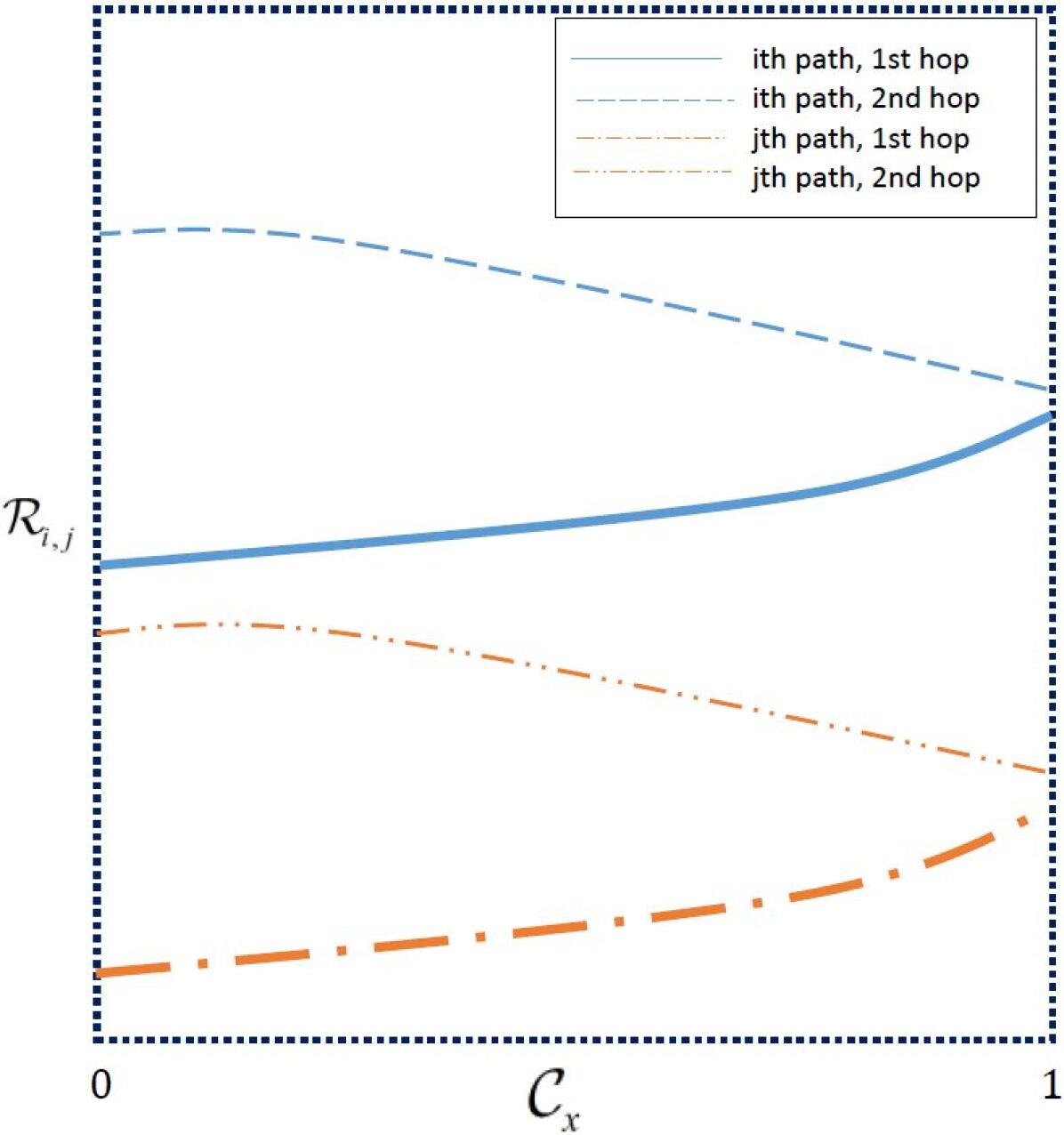
(a) The minimum rate functions are both increasing.

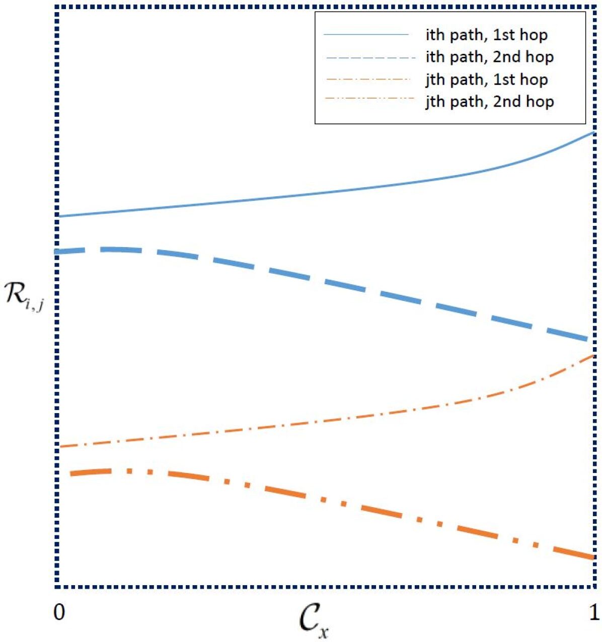
(b) The minimum rate functions are both decreasing.

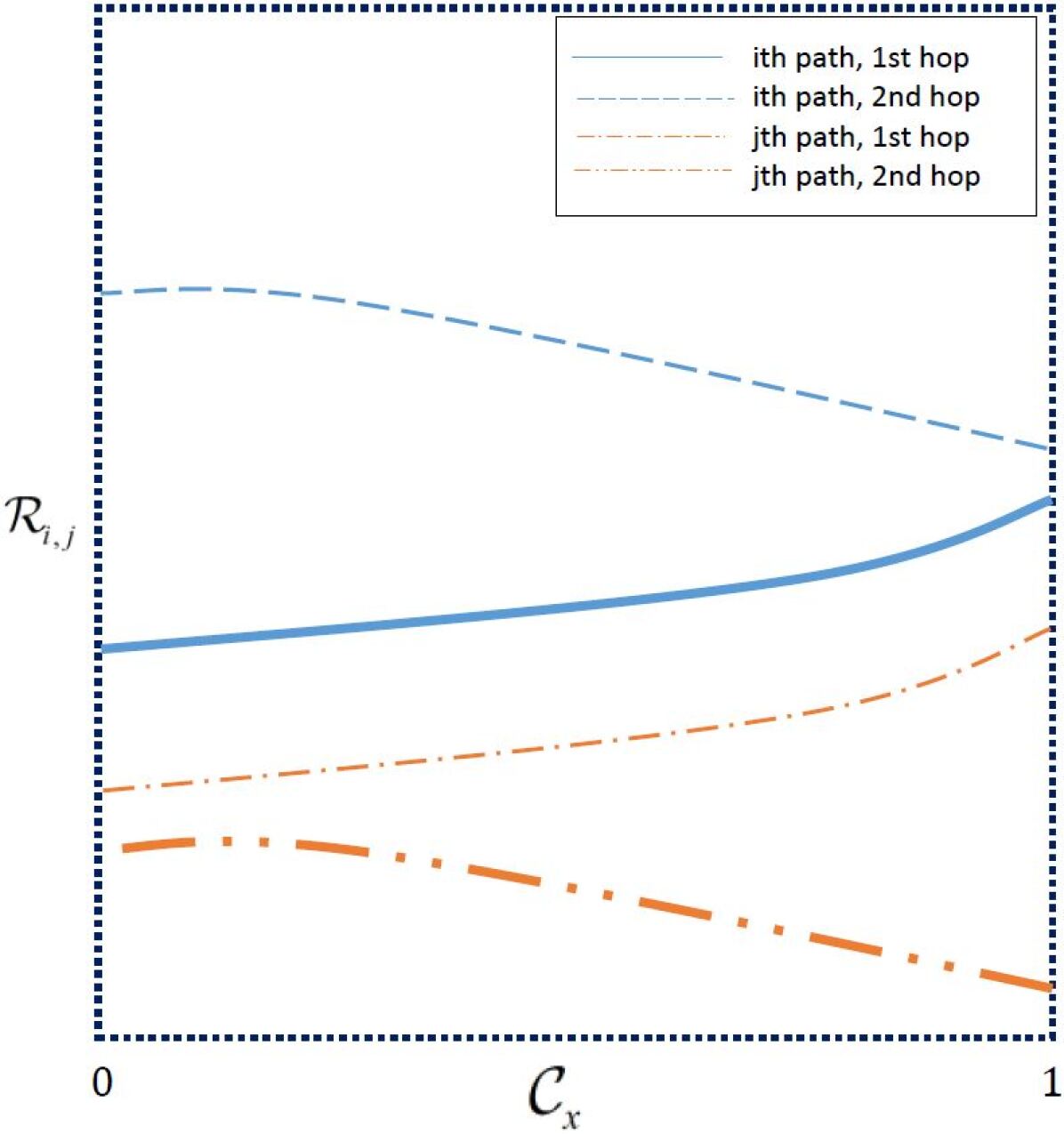
(c) The minimum rate functions are increasing and decreasing.

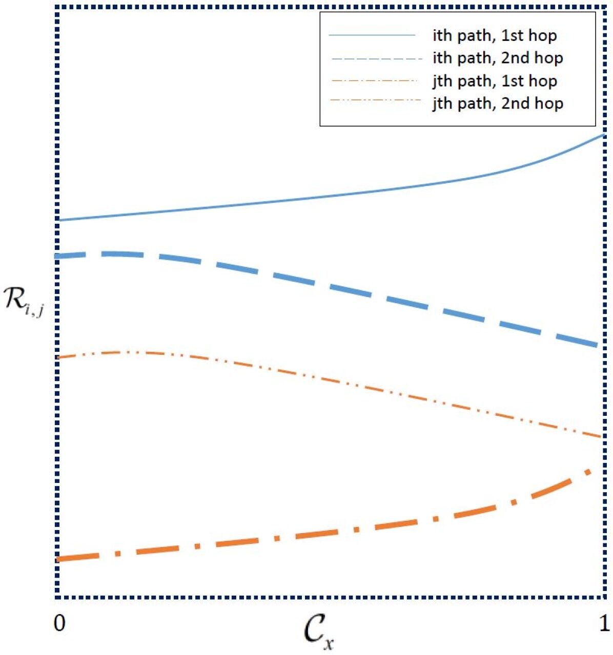
(d) The minimum rate functions are decreasing and increasing.

Figure 4: Possibilities for the rate functions configurations in case of no intersections between the 1st and 2nd hops of both paths (solid lines for the minumum rate function).

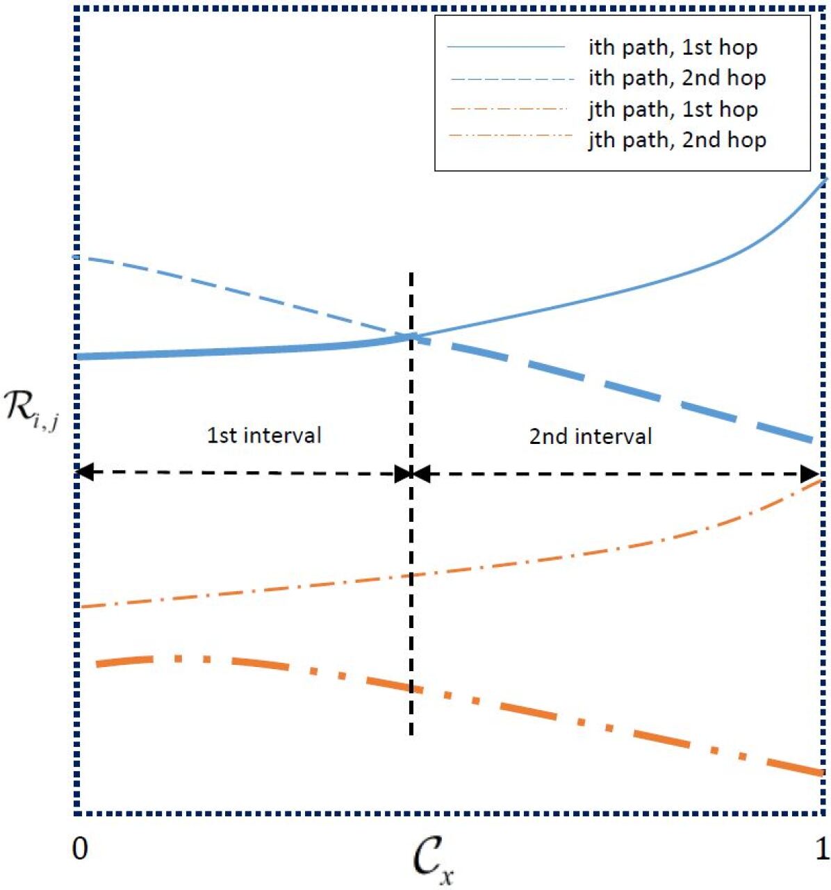
(a) The minimum rate function of the $j$th path is decreasing.

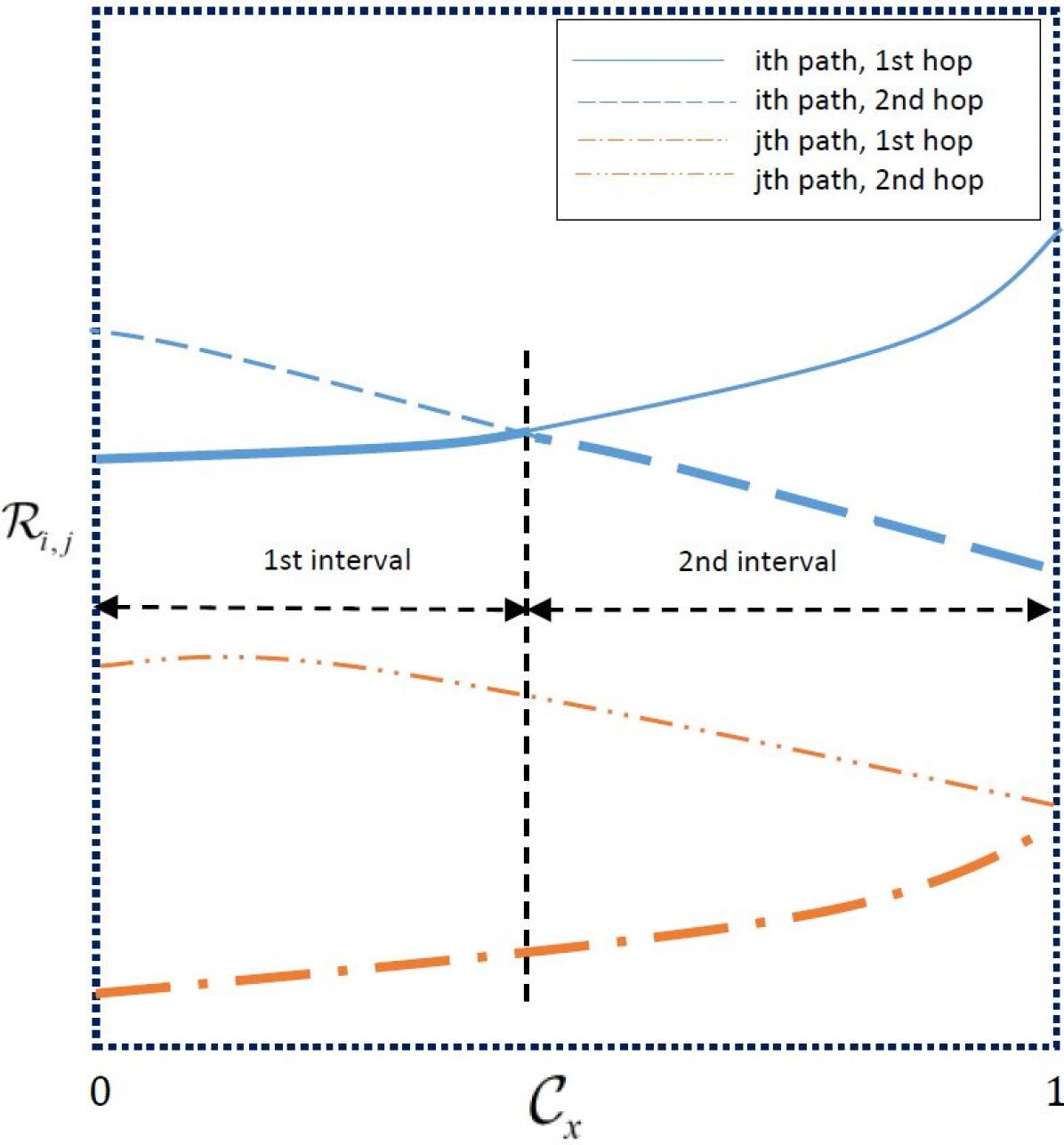
(b) The minimum rate function of the $j$th path is increasing.

Figure 5: Possibilities for the rate functions configurations in case of existence of intersection between the 1st and 2nd hops of only one of the paths (solid lines for the minumum rate function).

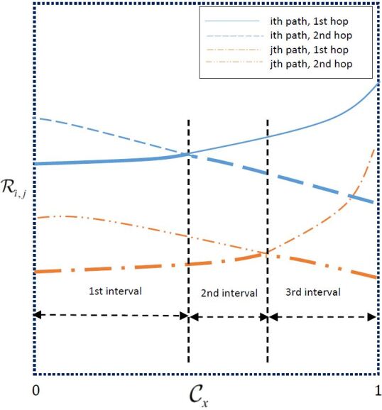
Figure 6: Possibilities for the rate functions configurations in case of existence of intersection between the 1st and 2nd hops of both paths (solid lines for the minumum rate function).

References

• [1] H. Ju, E. Oh, and D. Hong, “Catching resource-devouring worms in next-generation wireless relay systems: two-way relay and full-duplex relay,” IEEE Commun. Mag., vol. 47, no. 9, pp. 58–65, Sep. 2009.
• [2] C. Lameiro, I. Santamaria, and P. Schreier, “Benefits of improper signaling for underlay cognitive radio,” IEEE Wireless Commun. Lett., vol. 4, no. 1, pp. 22–25, Feb. 2015.
• [3] M. Gaafar, O. Amin, W. Abediseid, and M.-S. Alouini, “Spectrum sharing opportunities of Full-Duplex systems using improper Gaussian signaling,” in Proc. IEEE 26th Int. Symp. Personal, Indoor and Mobile Radio Communications (PIMRC), Hong Kong, Aug. 2015, pp. 244–249.
• [4] C. Lameiro, I. Santamaría, W. Utschiclk, and P. J. Schreier, “Maximally improper interference in underlay cognitive radio networks,” in Proc. IEEE Int. Conf. on Acoustics, Speech and Signal Processing (ICASSP), Mar. 2016, pp. 3666–3670.
• [5] O. Amin, W. Abediseid, and M.-S. Alouini, “Underlay cognitive radio systems with improper Gaussian signaling: Outage performance analysis,” IEEE Trans. Wireless Commun., vol. 15, no. 7, Jul. 2016.
• [6] M. Gaafar, O. Amin, W. Abediseid, and M.-S. Alouini, “Underlay spectrum sharing techniques with in-band full-duplex systems using improper Gaussian signaling,” IEEE Trans. Wireless Commun., vol. 16, no. 1, pp. 235–249, Jan. 2017.
• [7] O. Amin, W. Abediseid, and M.-S. Alouini, “Overlay spectrum sharing using improper Gaussian signaling,” IEEE J. Sel. Areas Commun., vol. 35, no. 1, pp. 50–62, Jan. 2017.
• [8] M. Gaafar, M. G. Khafagy, O. Amin, and M.-S. Alouini, “Improper Gaussian signaling in full-duplex relay channels with residual self-interference,” in Proc. IEEE Int. Conf. Commun. (ICC), Kuala Lumpur, Malaysia, May. 2016, pp. 1–7.
• [9] S. Lagen, A. Agustin, and J. Vidal, “Improper Gaussian signaling for the Z-interferece channel,” in Proc. IEEE Int. Conf. on Acoustics, Speech and Signal Processing (ICASSP), May 2014, pp. 1140–1144.
• [10] E. Kurniawan and S. Sun, “Improper Gaussian signaling scheme for the Z-interference channel,” IEEE Trans. Wireless Commun., vol. 14, no. 7, pp. 3912–3923, Jul. 2015.
• [11] S. Javed, O. Amin, S. S. Ikki, and M.S-Alouini, “Asymmetric hardware distortions in receive diversity systems: Outage performance analysis,” IEEE Access, to appear, 2017.
• [12] M. Gaafar, O. Amin, A. Ikhlef, A. Chaaban, and M. S. Alouini, “On alternate relaying with improper Gaussian signaling,” IEEE Commun. Lett., vol. 20, no. 8, pp. 1683–1686, Aug 2016.
• [13] M. Gaafar, O. Amin, R. F. Schaefer, and M.-S. Alouini, “Improper Signaling for Virtual Full-Duplex Relay Systems,” in Proc. 21st International ITG Workshop on Smart Antennas (WSA). to appear, Berlin, Germany, Mar. 2017. [Online]. Available: https://arxiv.org/abs/1702.04203
• [14] F. D. Neeser and J. L. Massey, “Proper complex random processes with applications to information theory,” IEEE Trans. Inf. Theory, vol. 39, no. 4, pp. 1293–1302, Jul. 1993.
• [15] Y. Zeng, C. M. Yetis, E. Gunawan, Y. L. Guan, and R. Zhang, “Transmit optimization with improper Gaussian signaling for interference channels,” IEEE Trans. Signal Process., vol. 61, no. 11, pp. 2899–2913, Jun. 2013.
• [16] V. R. Cadambe and S. A. Jafar, “Interference alignment and spatial degrees of freedom for the k user interference channel,” in Proc. IEEE Int. Conf. Communications (ICC), May 2008, pp. 971–975.
• [17] D. P. Bertsekas, Nonlinear Programming.   Athena Scientific, 1999.
• [18] C. Gerolamo, Ars Magna or the Rules of Algebra.   Dover, 1993.
• [19] V. V. Prasolov, Polynomials.   Springer Science & Business Media, 2009.