Inference of the chromospheric magnetic field orientation in the Ca ii 8542 Å line fibrils

Abstract

Context. Solar chromospheric fibrils, as observed in the core of strong chromospheric spectral lines, extend from photospheric field concentrations suggesting that they trace magnetic field lines. These images have been historically used as proxies of magnetic fields for many purposes.

Aims. Use statistical analysis to test whether the association between fibrils and magnetic field lines is justified.

Methods. We use a Bayesian hierarchical model to analyze several tens of thousands of pixels in spectro-polarimetric chromospheric images of penumbrae and chromospheric fibrils. We compare the alignment between the field azimuth inferred from the linear polarization signals through the transverse Zeeman effect and the direction of the fibrils in the image.

Results. We conclude that, in the analyzed fields of view, fibrils are often well aligned with the magnetic field azimuth. Despite this alignment, the analysis also shows that there is a non-negligible dispersion. In penumbral filaments, we find a dispersion with a standard deviation of $\sim 16^{\circ}$, while this dispersion goes up to $\sim 34^{\circ}$ in less magnetized regions.

1 Introduction

The solar chromosphere can be observed in the core of strong lines with sufficient opacity to be sensitive to the physical conditions above the photosphere (e.g., H$\alpha$, Ca ii H & K, Ca ii infrared triplet, Mg ii h & k). It can also be observed in the He i D₃ and $\lambda 10830$ lines which are influenced by ultraviolet photons from the corona (Centeno et al. 2008). In active regions, these images at the core of strong lines show a conspicuous filamentary structure fanning out from photospheric magnetic field concentrations, suggesting that they trace the magnetic field lines. This makes fibrils a natural proxy for the magnetic field orientation. Similar fibrils are observed in the umbra, penumbra and superpenumbra of sunspots with a very dynamic behaviour (see Rouppe van der Voort & de la Cruz Rodríguez 2013 and Yurchyshyn et al. 2014).

The relation between fibrils and magnetic field lines is appealing and intuitive. However, to our knowledge, very few studies have tried to establish this assumption. The main reason is the low polarimetric noise of the spectropolarimetric observations required to obtain quantitative information of the magnetic field vector. This explains why the very few observational attempts to test this assumption have been performed in penumbrae and superpenumbrae of sunspots, where polarized signals are generally stronger. To this aim, de la Cruz Rodríguez & Socas-Navarro (2011) used datasets in the Ca ii $\lambda 8542$ line whereas Schad et al. (2013) and Schad et al. (2015) used He i $\lambda 10830$ observations. The magnetic field vector inferred from these observations confirm, in most cases, the alignment between fibrils and the magnetic field, although de la Cruz Rodríguez & Socas-Navarro (2011) found cases of considerable misalignment in their Ca ii data.

In particular, de la Cruz Rodríguez & Socas-Navarro (2011) compared the visual orientation of fibrils with the inferred azimuth obtained from Zeeman-induced linear polarization measurements in the spectral line. The inherently noisy Stokes $Q$ and $U$ profiles (linear polarization appears at second order in the magnetic field in the Zeeman effect) forced them to average the Stokes parameters along a non-negligible length of the fibrils to improve the signal-to-noise ratio.

Leenaarts et al. (2015) studied the properties of fibrils using a 3D numerical simulation. The authors computed magnetic field lines starting at many seed points in the photosphere, and compared the orientation of the field with the 3D orientation of the fibrils where they found optical depth unity in the core of the H$\alpha$ line. They concluded that fibrils in the simulation are mostly aligned with the horizontal component of the magnetic field, but not necessarily always aligned with the vertical component. More recently, Martínez-Sykora et al. (2016), using radiative magneto-hydrodynamic simulations with a generalized Ohm’s law, have shown that the magnetic field is often not precisely aligned with chromospheric fibrils in places were the ambipolar diffusion is large. This is a consequence of the slip between the field lines and the neutral species produced by the decoupling between neutrals and ions.

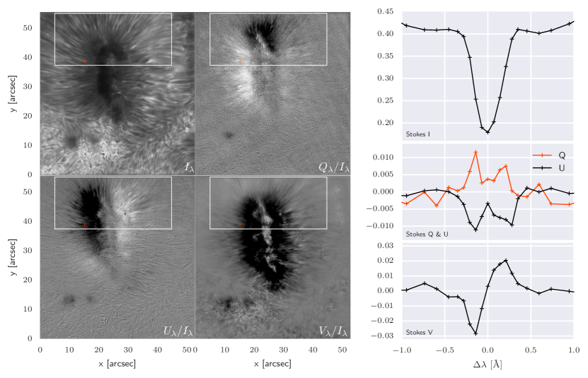
Figure 1: Left: Clockwise the panels show Stokes $I$, $Q$, $U$ and $V$ images at $\Delta\lambda=-140$ mÅ from line center in the Ca ii 8542 line for the observation of the penumbra. The analysis has been carried out in the subfield indicated with a white rectangle. Right: Full-Stokes spectra corresponding to the pixel indicated with a red marker in the FOV.

From an observational point of view, this work improves over that of de la Cruz Rodríguez & Socas-Navarro (2011) by utilizing more advanced techniques and better observations that allow us to analyze all relevant pixels in the image, increasing the statistics to several tens of thousands pixels, thus avoiding any averaging. The first improvement is the application of the rolling Hough transform (Clark et al. 2014) to estimate the direction of the fibrils in all the pixels. The second improvement is the application of a fully Bayesian hierarchical model (Gelman & Hill 2007) for the estimation of the statistical properties of the misalignment distribution.

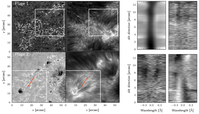
Figure 2: Plage observations, marking the analyzed region with a rectangle. The left panel shows the images in the continuum (left column) and in the core of the Ca ii 8582 Å line. The right panel displays an artificial slit along the orange line for Plage 2.

2 Polarimetric data

We consider spectropolarimetric observations of a penumbra and two plages around AR11793 recorded on July 19 and 22, 2013. The observations on July 19 started at 8:15 UT (plage) and 13:33 UT (penumbrae) at heliocentric distance $\mu=0.91$, while the observation at July 22 (plage 2) started at 08:33 UT at heliocentric distance $\mu=0.90$. Both datasets were obtained with the CRisp Imaging Spectro-Polarimeter (CRISP, Scharmer et al. 2008), a dual Fabry-Perot interferometer mounted in telecentric configuration at the Swedish 1-m Solar Telescope (SST, Scharmer et al. 2003). The spatial sampling is 0.059 arcsec/pixel. The data were processed using the CRISPRED package (de la Cruz Rodríguez et al. 2015). The seeing on July 19 was very good and no extra compensation for the atmospheric aberrations is applied. On the contrary, the Multi-Object, Multi-Frame Blind-Deconvolution technique (MOMFBD; Löfdahl & Scharmer 1994; van Noort et al. 2005) is applied to the data of July 22. The MOMFBD technique can enhance the noise even though a spatial filtering is applied to reduce this effect. For this reason, we consider that it is advisable to use non-corrected data for a quantitative analysis of the Stokes profiles if they are expected to be very close or even below the noise level. The polarimetric calibration was performed independently for each pixel of the field of view (FOV) as proposed by van Noort & Rouppe van der Voort (2008). Finally, we selected observations very close to disk center for an easier identification of linear polarization signals with the real azimuth of the magnetic field (thus avoiding line-of-sight effects).

The Ca ii $\lambda 8542$ Å was sampled in the range $\pm 1.75$ Å from the core of the line in 21 steps of different size: 70 mÅ close to the Doppler core of the line, 100 mÅ in the wings close to the core of the line, and 140 mÅ in the far wings. The sampling is thus almost a factor 2.3 better than that of the CRISP dataset used by de la Cruz Rodríguez & Socas-Navarro (2011) and the exposure time is also twice as long (400 ms total integration time taking into account the 4 modulation states). The resulting noise level is in the range $4-6\times 10^{-3}$ in units of the continuum intensity for Stokes $Q$, $U$ and $V$. The upper left panel of Fig. 1 shows an example of the monochromatic image in the core of the line for the penumbra observation, where we clearly distinguish the fibrils that are assumed to be associated with magnetic field lines. In this study we have selected the limb-side of the sunspot (indicated with a rectangle) because the Stokes $Q$ and $U$ signals are stronger there than in any other part of the FOV. The plage observations are summarized in Fig. 2. Because the signals are lower, in this case we show an artificial slit along the orange line to help the reader distinguish the presence of polarimetric signals. One can easily see Stokes $V$ signals close to the footpoints, and linear polarization in between, something that is to be expected. This figure also shows that above the bright points the Stokes $V$ signal appears in the photospheric wings (position 3” along the slit), but in general the polarization signals appear close to the chromospheric core of the line.

To interpret the polarimetric signals, we consider that the magnetic field strength is sufficiently weak that the Stokes parameters are formed in the so-called weak-field regime (Landi Degl’Innocenti & Landi Degl’Innocenti 1973). In this regime, the Zeeman splitting, $\Delta\lambda_{B}$, is much smaller than the Doppler broadening, $\Delta\lambda_{D}$ (e.g., Landi Degl’Innocenti & Landolfi 2004). For a very broad line such as the infrared Ca ii 8542 Å line, this assumption is usually appropriate (de la Cruz Rodríguez et al. 2013), especially given that we are sensing the magnetic field in the chromosphere, which is expected to be weaker than in the photosphere. In this case, the weak-field approximation allows one to compute the magnetic field vector much faster than with a depth-stratified non-LTE inversion where even the isotopic splitting of the Ca ii $8542$ line must be taken into account (Socas-Navarro et al. 2000; Leenaarts et al. 2014). Although based on quite strong simplifying assumptions (Landi Degl’Innocenti & Landolfi 2004) a reasonably accurate magnetic field azimuth is still obtained. Under this approximation, the linear polarization profiles $Q$ and $U$ are given by the following expressions (where all the quantities are constant along the line of sight):

$$Q_{w}(\lambda) =\beta_{w}B_{\perp}^{2}\left[\frac{\partial I(\lambda)}{\partial\lambda}\frac{1}{\lambda-\lambda_{0}}\right]_{w}\cos 2\phi,$$

$$U_{w}(\lambda) =\beta_{w}B_{\perp}^{2}\left[\frac{\partial I(\lambda)}{\partial\lambda}\frac{1}{\lambda-\lambda_{0}}\right]_{w}\sin 2\phi,$$ (1)

which are only valid on the wings of the line, as indicated with the subindex $w$. We choose the ranges $[-350,-140]$ mÅ and $[140,350]$ mÅ to compute these quantities, which are sufficiently far away from the line core but some Stokes $Q$ and $U$ signal is still measurable. Additionally, and according to Quintero Noda et al. (2016), these wing signals do still have a strong chromospheric contribution, with the response functions peaking very high in the atmosphere.

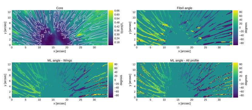
Figure 3: Upper left panel: image at the core of the Ca ii line in units of the average continuum intensity in the quietest region of the map. Upper right panel: estimated fibril angle using the RHT in the considered pixels. Lower panels: maximum-likelihood estimation of the azimuth angle obtained from the Stokes $Q$ and Stokes $U$ signal using only wavelengths on the wings (left panel) or the full line profile (right panel).

In the previous equations, $\beta_{w}=1.63\times 10^{-25}\bar{G}\lambda_{0}^{4}$ is a constant that depends on the specific spectral line of interest, with $\bar{G}$ the second order effective Landé factor for linear polarization (cf. Landi Degl’Innocenti & Landolfi 2004) and $\lambda_{0}$ the central wavelength of the line. Additionally, $B_{\perp}$ is the component of the magnetic field transverse to the line-of-sight (LOS), $\phi$ is the azimuth of the field in the plane perpendicular to the LOS, $\lambda$ is the wavelength and $I(\lambda)$ is the Stokes $I$ profile of the spectral line. Note that the numerical factor is valid if the field is measured in G and the wavelength in Å. The observed Stokes $Q$ and $U$ have been conveniently rotated so that the axis for which Stokes $Q>0$ (defined by the projection of the axis of the polarimetric analyzer on the plane-of-the-sky) lies along the vertical direction in the maps of Fig. 3.

One might also work with similar expressions that are valid on the entire line profile under more restrictive assumptions (see p. 407 of Landi Degl’Innocenti & Landolfi 2004). Such expressions are proportional to the second derivative of the intensity profile with respect to wavelength:

$$Q(\lambda) =-\beta B_{\perp}^{2}\left[\frac{\partial^{2}I(\lambda)}{\partial\lambda^{2}}\right]\cos 2\phi,$$

$$U(\lambda) =-\beta B_{\perp}^{2}\left[\frac{\partial^{2}I(\lambda)}{\partial\lambda^{2}}\right]\sin 2\phi,$$ (2)

where now $\beta=5.45\times 10^{-26}\bar{G}\lambda_{0}^{4}$. All the subsequent calculations have been obtained using Eqs. (1), which gives less noisy results, as demonstrated in Fig. 3.

Using the formulation worked out by Martínez González et al. (2012), we estimated the maximum-likelihood value of the azimuth at each considered pixel. The results are displayed in the lower panels of Fig. 3. These results suggest an overall good alignment between azimuth angle and fibril direction but no information on the observational uncertainties has been considered in the analysis.

3 Detection of fibrils

To compare the field orientation inferred from the polarimetry to that from the fibrils, we need to have a reliable estimate of the fibril direction in all relevant pixels. To this end, we make use of the recently presented rolling Hough transform (RHT, Clark et al. 2014), developed for detecting fibrils and estimating their direction in images of the interstellar medium. The RHT is a generalization of the standard Hough transform and is obtained after the following steps:

• A smoother version of the image is computed and then substracted from the original image. The smoothing is obtained using a top-hat kernel of a certain width $D_{K}$, which acts as a high-pass filter to suppress large scales.

• The resulting image is then thresholded and binarized to create a bitmask.

• A disk of a certain diameter $D_{W}$ is extracted at every point in the image and the standard Hough transform is computed in each disk.

• Finally, the Hough transform for each disk is thresholded at a certain level $Z$ to make sure that only obvious fibrils are detected as such.

As a consequence of its definition, the RHT is specially indicated to detect structures whose length is equal or longer than $D_{W}$ and with a brightness contrast larger than the threshold $Z$. This is specially suitable for the relatively diffuse images of the core of the Ca ii line (see Clark et al. 2014 for more details).

The output of the rolling Hough transform is the discretized function $R(\theta,x,y)$, which is defined at each pixel position $(x,y)$ and angle $\theta$. This function describes, for each disk of diameter $D_{W}$ centered at position $(x,y)$, the angles of the dominant linear structures. A visualization of the linear structures can be obtained by computing the backprojection $R(x,y)$, defined as:

$$R(x,y)=\int R(\theta,x,y)\,\mathrm{d}\theta.$$ (3)

Assuming that there is a preferential linear structure, the dominant azimuth at each pixel position is obtained by computing the circular statistics average at each pixel:

$$\phi_{\mathrm{RHT}}=\frac{1}{2}\arctan\frac{\int R(\theta,x,y)\sin(2\theta)\mathrm{d}\theta}{\int R(\theta,x,y)\cos(2\theta)\mathrm{d}\theta}.$$ (4)

The upper right panel of Fig. 3 displays the angle of each linear structure in the penumbra as obtained applying the RHT to the image on the upper left panel of the same figure. We found that using $D_{K}=10$, $D_{W}=55$ and $Z=0.7$ gives very good results but the results are not strongly dependent on small variations around these values. The reference angle is along the vertical direction. The umbra is removed from the azimuth map using a mask. In summary: we select dark structures in the map of the core brightness, we avoid the darkest regions in the continuum image to remove the umbra and we only choose points with a backprojection larger than 20% of the maximum (so that we only choose structures with a well-defined linear appearance). Once the dark filamentary structures are selected, the bright features are also trivially obtained as just the negative of the chosen mask (always discarding the umbra). We considered both the bright and dark structures in our analysis.

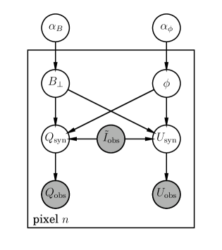
Figure 4: Graphical model representing the conditional dependences among the variables of the statistical model.

4 Inference of magnetic field azimuth

4.1 Bayesian hierarchical model

Under the presence of uncorrelated Gaussian noise, it is straightforward to write down the generative model used for explaining the linear polarization in the wings of the Ca ii line at the $j=1,\ldots,N_{\lambda}$ sampled wavelengths and for a given pixel $i=1,\ldots,N_{\mathrm{pix}}$. We modify Eqs. (1) to include the fibril angle estimated with the RHT and rechristen the azimuth to represent the misalignment between the magnetic field azimuth and the fibril direction:

$$Q_{ij} =\beta_{w}{B_{\perp}}_{i}^{2}\tilde{I}_{ij}\cos\left[2(\phi_{i}+\phi_{\mathrm{RHT},i})\right]+\epsilon_{Q,ij},$$

$$U_{ij} =\beta_{w}{B_{\perp}}_{i}^{2}\tilde{I}_{ij}\sin\left[2(\phi_{i}+\phi_{\mathrm{RHT},i})\right]+\epsilon_{U,ij},$$ (5)

where, for the sake of a simpler notation, we use $\tilde{I}(\lambda)=(\partial I/\partial\lambda)/(\lambda-\lambda_{0})$, with the numerical derivatives being calculated using a quadratic Lagrangian interpolation. Note that, when $\phi_{i}=0$, one can safely state that the magnetic field is along the fibril direction.

We acknowledge that our treatment of noise is somehow simplified. We assume that the noise contributions, $\epsilon_{Q,ij}$ and $\epsilon_{U,ij}$, are Gaussian-distributed random variables with zero mean and standard deviation $\sigma_{n}$. The standard deviation is estimated from the continuum wavelengths on the observations, where the linear polarization signal is expected to be zero. We find $\sigma_{n}\sim 5-7\times 10^{-3}I_{c}$, where $I_{c}$ is the continuum intensity. Under this framework, we are assuming that all sources of error (photon noise, uncertainty in the estimation of the fibril angle, fringes and any other systematic effect) are absorbed in these zero mean errors with variances empirically obtained from the data. Another particularity of our generative model is that it depends on an observed (and, consequently, noisy) quantity, $\tilde{I}(\lambda)$. According to Asensio Ramos & Manso Sainz (2011), in such a case the noise variance should take this into account. For the moment, we neglect this second order effect in this work and we defer a more elaborate Bayesian treatment of all systematic and random uncertainties for a future publication.

If we analyze a single pixel $i$, the information about ${B_{\perp}}_{i}$ and $\phi_{i}$ that can be extracted from the observations is summarized in the posterior distribution:

$$p(\phi_{i},{B_{\perp}}_{i}|\tilde{\mathbf{I}}_{i},\mathbf{Q}_{i},\mathbf{U}_{i})=p(\tilde{\mathbf{I}}_{i},\mathbf{Q}_{i},\mathbf{U}_{i}|\phi_{i},{B_{\perp}}_{i})p({B_{\perp}}_{i})p(\phi_{i}),$$ (6)

where $p(\tilde{\mathbf{I}}_{i},\mathbf{Q}_{i},\mathbf{U}_{i}|\phi_{i},{B_{\perp}}_{i})$ is the likelihood associated to pixel $i$ (with $\tilde{\mathbf{I}}_{i}$, $\mathbf{Q}_{i}$ and $\mathbf{U}_{i}$ vectors containing all the observed wavelengths for the pixel). Likewise, $p({B_{\perp}}_{i})$ and $p(\phi_{i})$ are priors that are assumed to be independent for all pixels. Applying this scheme to all pixels in the FOV, one may estimate the diversity in the misalignments by comparing their posteriors.

However, it is useful to make the assumption that all pixel share a common prior and use a hierarchical model to put together all the partial and uncertain information from each pixel to constrain this prior (e.g., Brewer & Elliott 2014). In other words, even though each pixel is characterized by ${B_{\perp}}_{i}$ and $\phi_{i}$, we put a common parametric prior that depends on the set of hyperparameters $\alpha_{\phi}$ and $\alpha_{B}$. These priors are shared by all pixels in the field-of-view (FOV). Using simple rules of probability calculus, it is easy to write the posterior distribution for all pixels simultaneously:

$$p(\mbox{\boldmath$\phi$},\mathbf{B}_{\perp},\alpha_{\phi},\alpha_{B}|\tilde{\mathbf{I}},\mathbf{Q},\mathbf{U}) =p(\tilde{\mathbf{I}},\mathbf{Q},\mathbf{U}|\mbox{\boldmath$\phi$},\mathbf{B}_{\perp})$$

$$p(\mathbf{B}_{\perp}|\alpha_{B})p(\alpha_{B})p(\mbox{\boldmath$\phi$}|\alpha_{\phi})p(\alpha_{\phi}),$$ (7)

which is trivially inferred from the graphical model displayed in Fig. 4. In the previous equation, $\tilde{\mathbf{I}}$, $\mathbf{Q}$ and $\mathbf{U}$ contain all the observations for all pixels. As seen from the previous expression, the model includes a hierarchical prior for $\phi$, which is made dependent on the set of hyperparameters $\alpha_{\phi}$ (over which we set another prior to be consistent with the Bayesian framework). Given the assumption of uncorrelated noise in all pixels, the likelihood can be written as (see Appendix A):

$$p(\tilde{\mathbf{I}},\mathbf{Q},\mathbf{U}|\mbox{\boldmath$\phi$},\mathbf{B}_{\perp})=\prod_{i=1}^{N_{\mathrm{pix}}}\mathcal{L}_{Q,i}(\phi_{i},{B_{\perp}}_{i})\,\mathcal{L}_{U,i}(\phi_{i},{B_{\perp}}_{i}),$$ (8)

with

$$\mathcal{L}_{Q,i}(\phi_{i},{B_{\perp}}_{i}) =\prod_{j=1}^{N_{\lambda}}p(\tilde{I}_{ij},Q_{ij}|\phi_{i},{B_{\perp}}_{i})$$

$$\mathcal{L}_{U,i}(\phi_{i},{B_{\perp}}_{i}) =\prod_{j=1}^{N_{\lambda}}p(\tilde{I}_{ij},U_{ij}|\phi_{i},{B_{\perp}}_{i}).$$

Given that our interest is to obtain statistical information about the azimuth in the whole FOV and we are not really interested in their specific values for individual pixels, we marginalize $\phi$ and $\mathbf{B}_{\perp}$ from the posterior distribution of Eq. (7):

$$p(\alpha_{\phi},\alpha_{B}|\tilde{\mathbf{I}},\mathbf{Q},\mathbf{U})=\int\mathrm{d}\mbox{\boldmath$\phi$}\mathrm{d}\mathbf{B}_{\perp}p(\mbox{\boldmath$\phi$},\mathbf{B}_{\perp},\alpha_{\phi},\alpha_{B}|\tilde{\mathbf{I}},\mathbf{Q},\mathbf{U}).$$ (9)

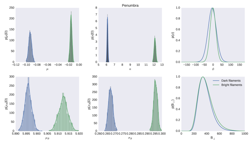
Figure 5: The first and second columns show the marginal posterior for the hyperparameters of the von-Mises prior for the misalignment (upper panels) and the log-normal prior for the perpendicular component of the magnetic field (lower panels) for the case of the penumbra. The plots show a histogram and a kernel density estimation using the samples. The rightmost column shows the Montecarlo estimate of the prior distribution for all considered pixels for both parameters.

4.2 Priors and hyperpriors

The problem is fully defined once we set the parametric priors $p(\phi_{i}|\alpha_{\phi})$ and $p(B_{\perp}|\alpha_{B})$, and the hyperpriors $p(\alpha_{\phi})$ and $p(\alpha_{B})$. Concerning the prior for the misalignment, we choose a von-Mises distribution, which is naturally defined on the interval $[-\pi,\pi]$ and is also naturally periodic. The von-Mises distribution is one of the most used generalizations of the normal distribution for circular statistics and is quite flexible. Its functional form is:

$$p_{\mathrm{VM}}(\phi_{i}|\mu,\kappa)=\frac{1}{2\pi I_{0}(\kappa)}\exp\left[\kappa\cos\left(\phi_{i}-\mu\right)\right],$$ (10)

which depends on the set of hyperparameters $\alpha_{\phi}=(\mu,\kappa)$. In the previous expression, $I_{i}(\kappa)$ is the modified Bessel function of the first kind (Abramowitz & Stegun 1972). As $\kappa$ increases, the von-Mises distribution approaches a normal distribution with the same mean and standard deviation $\sigma=\sqrt{2}/\kappa$. To finalize, a suitable Jeffreys’-type hyperprior $p(\mu,\kappa)$ is given by (Dowe et al. 1996):

$$p(\mu,\kappa)\propto\left[\kappa A(\kappa)\frac{\mathrm{d}A(k)}{\mathrm{d}k}\right]^{1/2},$$ (11)

with $A(\kappa)=I_{1}(\kappa)/I_{0}(\kappa)$. However, we have checked that the more standard Jeffreys’ prior $p(\mu,\kappa)\propto\sigma^{-1}$ also works equivalently in our case (e.g., Gregory 2005). For computational reasons, we have used the almost equivalent inverse Gamma prior

$$\mathrm{IG}(\sigma;\alpha,\beta)=\frac{\beta^{\alpha}}{\Gamma(\alpha)}\sigma^{-\alpha-1}\exp\left(\frac{-\beta}{\sigma}\right)$$ (12)

which converges to the Jeffreys’ prior when $\alpha\ll 1$ and $\beta\ll 1$.

To complete the problem, we choose a log-normal distribution for $B_{\perp,i}$:

$$p_{\mathrm{LN}}(B_{\perp,i}|\mu,\kappa)=\frac{1}{B_{\perp,i}\sqrt{2\pi}\sigma_{B}}\exp\left[-\frac{\left(\log B_{\perp,i}-\mu_{B}\right)^{2}}{2\sigma_{B}^{2}}\right],$$ (13)

which is parameterized by the location $\mu_{B}$ and scale $\sigma_{B}$ parameters, $\alpha_{B}=(\mu_{B},\sigma_{B})$. Additionally, we set a standard Jeffreys’ prior $p(\mu,\kappa)\propto\sigma_{B}^{-1}$ through an inverse Gamma prior. The log-normal distribution naturally puts zero probability to $B_{\perp,i}=0$, which arises naturally from a non-pathological vector field in three dimensions.

4.3 Variational method

The computation of the marginalization integral can be potentially carried out using Markov Chain Monte Carlo techniques. However, given the large number of pixels we want to analyze, the integration becomes very time consuming. For this reason, we use an automatic variational approximation, as included in the Stan software (Kucukelbir et al. 2015). Variational inference relies on using a simpler parametric distribution to approximate the posterior distribution. In short, assume that our aim is to approximate the posterior distribution $p(\mbox{\boldmath$\theta$}|\mathbf{X})$, where $\theta$ is the vector of parameters and $\mathbf{X}$ are the observations. If one considers the family $q(\mbox{\boldmath$\theta$}|\mbox{\boldmath$\phi$})$ of probability densities parameterized by the vector $\phi$, it is possible to obtain an approximation to the posterior by computing the value of the parameters that give a smaller value of the Kullback-Leibler divergence, $D_{\mathrm{KL}}$, between the two distributions (e.g., Bishop 2006):

$$\operatorname*{arg\,min}_{\mbox{\boldmath$\phi$}}D_{\mathrm{KL}}[q(\mbox{\boldmath$\theta$}|\mbox{\boldmath$\phi$})\parallel p(\mbox{\boldmath$\theta$}|\mathbf{X})].$$ (14)

Since the Kullback-Leibler divergence usually lacks a closed form, it is customary to maximize a slightly different problem, in which the evidence lower bound ($L$) appears:

$$\operatorname*{arg\,max}_{\mbox{\boldmath$\phi$}}L(\mbox{\boldmath$\phi$})=\mathbb{E}_{q(\mbox{{\boldmath$\theta$}})}\left[\log p(\mbox{\boldmath$\theta$},\mathbf{X})\right]-\mathbb{E}_{q(\mbox{{\boldmath$\theta$}})}\left[\log q(\mbox{\boldmath$\theta$}|\mbox{\boldmath$\phi$})\right],$$ (15)

where $\mathbb{E}_{q(\theta)}[x]$ is the expectation value of $x$ over the distribution $q(\theta)$. The variational approximation greatly simplifies the problem and allows it to scale very well when the number of observations and/or variables increases. We use the implementation of the variational approximation included in the Stan package (Carpenter et al. 2016) .

5 Results

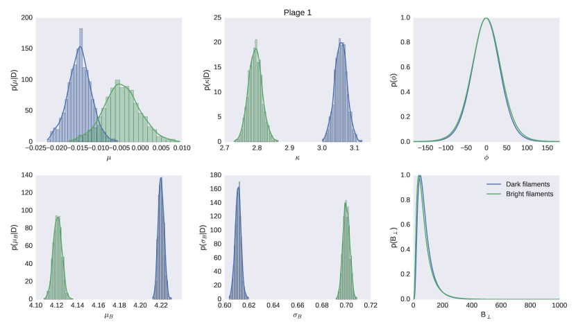
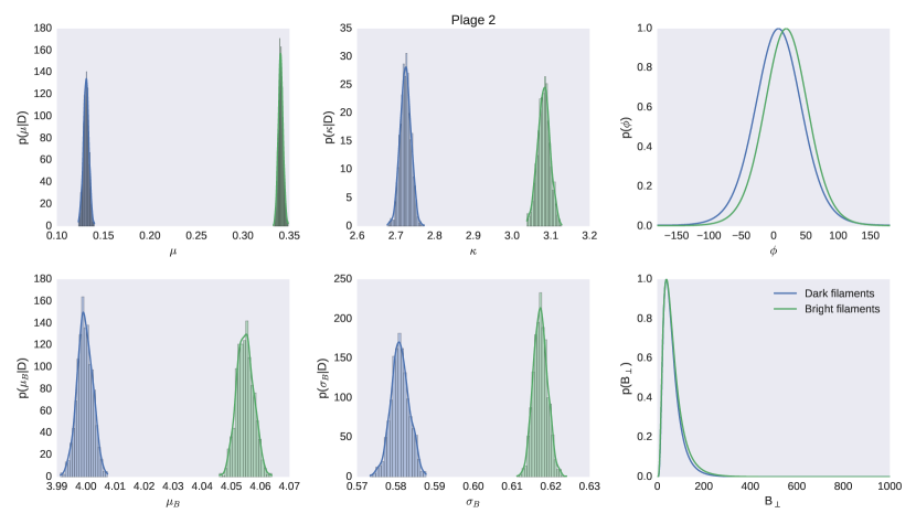
Figure 6: Same as Fig. 5 but for the two plages cases considered.

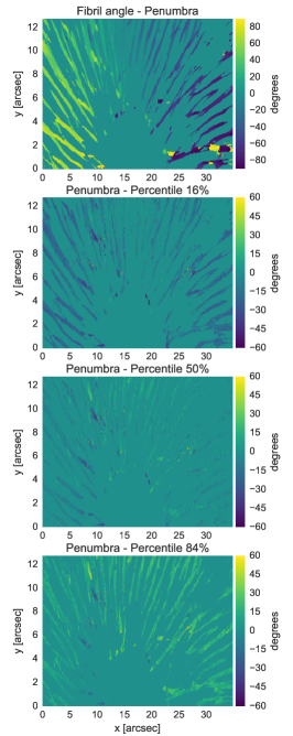
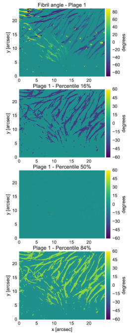
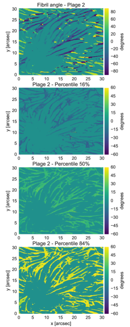
Figure 7: The upper row display the fibril angle inferred from the bright structures in the images at the core of the line. The second, third and last rows display the 16, 50 and 84 percentiles of the distribution of inferred misalignments for each pixel.

5.1 Penumbra

Our inference for the penumbra is based on a total of $\sim 3\times 10^{4}$ pixels of the map, both for the bright and dark structures. The marginal distributions for the hyperparameters of the von-Mises and log-normal distributions are displayed in the first and second columns of Fig. 5. Note that the marginal posteriors for the hyperparameters are very well defined for both the misalignment and the perpendicular component of the magnetic field. The distributions point to a slight statistical misalignment overall between the azimuth of the field and the fibril direction of less than $\sim 1^{\circ}$ for the bright structures, and less than $\sim 6^{\circ}$ for the dark ones. Although statistically relevant, it seems rather unimportant given that it is probably within the uncertainty in the determination of the fibril direction. Concerning the field, it points towards a median value for the perpendicular field of $e^{\mu_{B}}\sim 370$ G, compatible in both cases. This suggests that bright and dark structures are located in regions of relatively smooth magnetic field.

Motivated by the well-constrained values of the hyperparameters, it is advisable to use these samples to produce a Montecarlo estimate of the prior distribution over the whole field of view that we used. To this end, we compute the averaged distribution for the misalignment and field using:

$$\langle p(\phi)\rangle =\frac{1}{N}\sum_{i=1}^{N}p(\phi|\alpha_{\phi,i})\,,$$

$$\langle p(B_{\perp})\rangle =\frac{1}{N}\sum_{i=1}^{N}p(B_{\perp}|\alpha_{B_{\perp},i})\,,$$ (16)

where $N$ is the number of samples obtained from the variational approximation. The results are shown in the rightmost column of Fig. 5. Given that the values of $\kappa$ are large, the results are almost Gaussian. The dark structures show a mean of $\sim-6^{\circ}$ and a standard deviation of $\sim 23^{\circ}$, while the bright structures display a mean of $\sim-1^{\circ}$ and a standard deviation of $\sim 16^{\circ}$. In other words, we find that the probability of having a misalignment larger than 16^∘ in the bright filaments is only 32%. Additionally, the probability of finding a misalignment larger than 32^∘ goes down to 5%. A similar reasoning is applied to the dark structures. It is important to note, however, that these probabilities are all referred to the penumbra region observed here.

It is true that the results displayed in Fig. 5 depend on the number of pixel considered, with the distribution of hyperparameters slowly converging to a certain value when $N_{\mathrm{pix}}$ increases. The convergence of the means, $\mu$ and $\mu_{B}$, go roughly as $N_{\mathrm{pix}}^{1/2}$. This is the well-known behavior of the convergence of the mean when adding many samples. However, the convergence of the hyperparameters related with the dispersion is much slower. The reason is that these are already second-order statistics, and their uncertainty decreases as $N_{\mathrm{pix}}^{1/4}$. As a consequence, combining 3$\times$10⁴ pixels reduces the uncertainty in the mean by a factor $\sim 170$ with respect to the single-pixel case. Meanwhile, the uncertainty in the width of the distribution decreases only by a factor $\sim 13$. In other words, we can safely state that the mean value of the misalignment is close to zero, but our certainty in the dispersion is smaller. We have checked this experimentally by doing the analysis with several number of pixels from 1 to 3$\times$10⁴ and verifying that the value of $\mu$ rapidly converges toward 0, while the value of $\kappa$ is probably representative but not yet fully converged.

Using a common prior for all pixels introduces a shrinkage effect that pushes all inferred misalignments to share a common prior. This effect is seen in the leftmost column of Fig. 7, where we show the percentiles 16, 50 and 84 for the misalignment for all considered pixels, together with the map of fibril angles inferred with the RHT. The median value of the misaligmnent for all pixels is around zero for almost all fibrils, except in some specific locations. Additionally, the percentile 16 shows negative values almost all over the field of view, while the percentile 84 displays positive values. Of interest are the regions at (10$"$,9$"$), (7$"$,6$"$) and (8$"$,1$"$), that display a negative misalignment in all percentiles. The misalignments can be real or they can be produced by an incorrect estimation of the geometrical alignment of the fibril. We note that all these cases are fibrils that are not strictly along the remaining penumbra filaments, but are linking two parallel fibrils. Finally, the smooth appearance of the maps of Fig. 7 suggest that the dispersion found in the distributions of misalignments of Fig. 5 is intrinsic, and not produced by non-converged results for $\kappa$.

In other words, it is sure that the average misalignment is compatible with zero, but it is still unclear whether the dispersion found is produced by noise or it is real.

5.2 Plage

Although checking for the alignment of chromospheric fibrils and magnetic fields in penumbrae is interesting, it turns out to be even more important to check for this alignment in less magnetized regions. According to the recent simulations of Martínez-Sykora et al. (2016), ambipolar diffusion can often produce misalignments between the high-density weakly ionized fibrils and the magnetic field. For this reason, we also analyze regions above plages, whose results are displayed in Fig. 6 for the two cases considered in this work. The first plage contains $\sim$3$\times$10⁴ pixels for the bright filaments, and $\sim$5$\times$10⁴ pixels for the dark ones, while in the second one we increased the number of points to $\sim$6$\times$10⁴ for the bright structures and $\sim$5$\times$10⁴ for the dark ones. The inferred hyperparameters indicate that the field is almost aligned with the bright and dark structures in the first case. On the contrary, it turns out to be slightly misaligned ($\sim 19.5^{\circ}$ for bright structures and $\sim 7.5^{\circ}$ for dark ones) in the second case. Both share roughly the same uncertainty in the misalignment of $\sim 34^{\circ}$. Given that the Stokes $Q$ and $U$ signals in these regions have lower amplitudes than in the penumbra, we cannot discard that the estimated uncertainty in the misalignment can be reduced by adding many more pixels because it is still dominated by the presence of noise. Concerning the magnetic field perpendicular to the line-of-sight, the results consistently indicate that they are much smaller than in the penumbra, with median values equal to $e^{\mu_{B}}\sim 60$ G.

The shrinkage effect of the hierarchical model is demonstrated for the plage case in the middle and right columns of Fig. 7. We find no relevant regions in the maps with a strong misalignment.

6 Discussion and conclusion

To put these results in the context of previous work, let us recall that de la Cruz Rodríguez & Socas-Navarro (2011) obtained azimuths of the field (averaged along each fibril) that were, on average, well aligned with the direction of the fibrils. However, they also found a non-negligible fraction of the tens of cases analyzed where strong misalignments were observed, in some cases close to 90^∘. Our results do not indicate the presence of such strong differences, at least statistically. The discrepancy might be due to the presence of noise (de la Cruz Rodríguez et al. 2012), which affects the maximum likelihood estimation of the azimuth used by de la Cruz Rodríguez & Socas-Navarro (2011), or to the fact that the regions are different. Although less likely (but possible), the findings of Leenaarts et al. (2015) using 3D simulations seem to indicate that fibrils in H$\alpha$ do not necessarily trace the vertical component of the magnetic field, at least not where $\tau_{\mathrm{\lambda_{0}}}=1$. Therefore misalignments may occur in observations close to the limb, where Stokes $Q$ & $U$ signals would originate from the vertical component of the field due to projection effects. One of the datasets used by de la Cruz Rodríguez & Socas-Navarro (2011) is at heliocentric distance $\mu=0.41$. In the present work, the penumbra median misalignments could also produced by elevation effects along the fibrils. The potential misalignments that we find in this work (although the median value is very close to zero) might be compatible with the simulations of Martínez-Sykora et al. (2016). Therefore, observations with better signal-to-noise ratio are needed to observationally quantitatively pin down the importance of ambipolar diffusion producing strong misalignments between fibrils and the magnetic field.

Our results are also in good agreement with the findings of Schad et al. (2013) who used the He i $\lambda 10830$ line to measure the alignment of fibrils in the surrounding of a sunspot. Given that polarization in the Ca ii $\lambda 8542$ line can be modeled in active regions using (only) the Zeeman effect (Manso Sainz & Trujillo Bueno 2010) and it does not suffer from extra ambiguities in the azimuth derived from the Hanle effect and scattering polarization, our results also reinforce the findings of Schad et al. (2013) but (in our case) using a diagnostic from a completely different formation mechanism both for the line (different atom, optically thick) and for the polarization (Zeeman induced).

Appendix A Likelihood

Because all observed pixels and wavelengths are assumed to be uncorrelated, we can factorize the likelihood as follows:

$$p(\tilde{\mathbf{I}},\mathbf{Q},\mathbf{U}|\mbox{\boldmath$\phi$},\mathbf{B}_{\perp})=\prod_{i=1}^{N_{\mathrm{pix}}}\prod_{j=1}^{N_{\lambda}}p(\tilde{I}_{ij},Q_{ij}|\phi_{i},{B_{\perp}}_{i})p(\tilde{I}_{ij},U_{ij}|\phi_{i},{B_{\perp}}_{i}),$$ (17)

where the terms in the likelihood are given by the following normal distributions:

$$p(\tilde{I}_{ij},Q_{ij} |\phi_{i},{B_{\perp}}_{i})=$$

$$\frac{1}{\sqrt{2\pi}\sigma_{n}}\exp\left[-\frac{\left(Q_{ij}-\beta_{w}{B_{\perp}}_{i}^{2}\tilde{I}_{ij}\cos\left[2(\phi_{i}+\phi_{\mathrm{RHT},i})\right]\right)^{2}}{2\sigma_{n}^{2}}\right],$$ (18)

$$p(\tilde{I}_{ij},U_{ij} |\phi_{i},{B_{\perp}}_{i})=$$

$$\frac{1}{\sqrt{2\pi}\sigma_{n}}\exp\left[-\frac{\left(U_{ij}-\beta_{w}{B_{\perp}}_{i}^{2}\tilde{I}_{ij}\sin\left[2(\phi_{i}+\phi_{\mathrm{RHT},i})\right]\right)^{2}}{2\sigma_{n}^{2}}\right].$$ (19)

We note that the product over wavelengths can be computed analytically, and the resulting likelihoods are still normal:

$$\mathcal{L}_{Q,i} =\prod_{j=1}^{N_{\lambda}}p(\tilde{I}_{ij},Q_{ij}|\phi_{i},{B_{\perp}}_{i})\propto$$

$$\exp\left[-\frac{1}{2\sigma_{i}^{2}}\left(\frac{S_{QI,i}}{S_{I,i}}-\beta_{w}{B_{\perp}}_{i}^{2}\cos\left[2(\phi_{i}+\phi_{\mathrm{RHT},i})\right]\right)^{2}\right]$$ (20)

$$\mathcal{L}_{U,i} =\prod_{j=1}^{N_{\lambda}}p(\tilde{I}_{ij},U_{ij}|\phi_{i},{B_{\perp}}_{i})\propto$$

$$\exp\left[-\frac{1}{2\sigma_{i}^{2}}\left(\frac{S_{UI,i}}{S_{I,i}}-\beta_{w}{B_{\perp}}_{i}^{2}\sin\left[2(\phi_{i}+\phi_{\mathrm{RHT},i})\right]\right)^{2}\right],$$ (21)

where

$$S_{I,i}=\sum_{j=1}^{N_{\lambda}}\tilde{I}_{ij}^{2},\,\,S_{QI,i}=\sum_{j=1}^{N_{\lambda}}Q_{ij}\tilde{I}_{ij},\,\,S_{UI,i}=\sum_{j=1}^{N_{\lambda}}U_{ij}\tilde{I}_{ij},\,\,\sigma_{i}=\frac{\sigma_{n}}{\sqrt{S_{I,i}}}$$ (22)