The linear optical response of the quantum vacuum

Abstract

We show that the interpretation of $\mathbf{D}=\varepsilon_{0}\mathbf{E}$ as vacuum polarization is consistent with quantum electrodynamics. A free electromagnetic field polarizes the vacuum but the magnetization and polarization currents cancel giving zero source current. The speed of light is a universal constant while the fine structure constant that couples the EM field to matter runs. In that sense, the quantum vacuum can be understood as a modern Lorentz invariant ether.

1 Introduction

Quantum electrodynamics (QED) is the most successful theory in human history, but it is normally relegated to short range or high energy phenomena such as the Lamb shift, collisions of high energy particle beams and ultra-intense laser fields. Except for photon emission and absorption and the Casimir effect, its relevance to low-energy laboratory physics and every day life is unclear Milonni ; Boi .

Recently it has been proposed that $\mathbf{D=}\varepsilon_{0}\mathbf{E}$ is the vacuum polarization due to virtual pairs of all types of charged elementary particle in Nature LeuchsSS10 ; LeuchsSS13 ; Urban11 . This is a paradigm shift in our physical picture of the vacuum, but we will show here that this interpretation of $\varepsilon_{0}$ is consistent with QED.

In a dielectric material the electric displacement is $\mathbf{D}=\varepsilon_{0}\mathbf{E}+\mathbf{P}$, where $\mathbf{P}=\varepsilon_{0}\chi_{e}\mathbf{E}$ is the polarization due to the electric field $\mathbf{E}$ and $\chi_{e}$ is the electric susceptibility. If the material is magnetic the field strength is $\mathbf{H}=\mathbf{B}/\mu_{0}-\mathbf{M}$, where $\mathbf{B}$ is the magnetic flux density and $\mathbf{M}$ is the magnetization. A field independent dielectric permittivity $\varepsilon$ and magnetic permeability $\mu$ describe its linear response. The dependence of $\varepsilon$ and $\mu$ on the frequency plays a central role in applications and in some situations their dependence on wave vector can be significant Horsley . The relationship between $\mathbf{D}$ and $\mathbf{E}$ and between $\mathbf{H}$ and $\mathbf{B}$ is nonlocal in space and time, but local in reciprocal spacetime, where a dielectric permittivity $\varepsilon(\omega,\mathbf{k})$ and magnetic permeability $\mu(\omega,\mathbf{k})$ can be defined such that $\mathbf{D}(\omega,\mathbf{k})=\varepsilon(\omega,\mathbf{k})\mathbf{E}(\omega,\mathbf{k})$ and $\mathbf{H}(\omega,\mathbf{k})=\mathbf{B}(\omega,\mathbf{k})/\mu(\omega,\mathbf{k})$.

Consistency with the quantitative predictions of QED will be maintained here, but $\varepsilon_{0}$ and $\mu_{0}$ will be interpreted as the dielectric permittivity and magnetic permeability of vacuum. Vacuum has a crucial property that is does not share with dielectric and magnetic materials; it is Lorentz invariant. Due to this property Michaelson and Morley failed to detect the motion of the earth through the “ether”, which in the present context is the quantum vacuum. Empty spacetime is homogeneous so variations of $\varepsilon_{0}$ and $\mu_{0}$ can occur only in the presence of charged matter. The linear response of vacuum must be Lorentz invariant, so in reciprocal space the susceptibility of vacuum must be a function of $k^{2}=\omega^{2}/c^{2}-\mathbf{k}^{2}$.

The condition $k^{2}=0$ describing a freely propagating photon is referred to as on-shellness in QED. In relativity a particle with mass $m$ satisfying the dispersion relation $\omega^{2}=\mathbf{k}^{2}c^{2}+m^{2}c^{4}/\hbar^{2}$ is referred to as on-mass-shell or just on-shell. A real photon has zero mass, so for an on-shell photon $\omega^{2}=\mathbf{k}^{2}c^{2}.$

It is conventional in QED to use natural units with $\varepsilon_{0}$ set equal to $1$ for all values of $k^{2}$. In the dielectric model of vacuum presented here $\varepsilon_{0}$ and $\mu_{0}$ are functions of the off-shellness of the photon, $k^{2}$.

This paper is organized as follows: Section 2 describes vacuum polarization due to creation of virtual particle-antiparticle pairs. The dielectric model of the quantum vacuum is presented in Section 3. The interpretation of $\mathbf{D}$ as vacuum polarization is discussed in Section 4. Finally, our conclusions are summarized in Section 5.

2 Vacuum polarization

The Feynman diagrams in Fig. 1 are a pictorial representation of vacuum polarization in QED in the one-loop approximation. The wavy lines represent an electromagnetic (EM) field and a dot is a vertex where this EM field interacts with the fermions. The loop labelled $1$ represents a virtual electron-positron pair created at space-time point $x_{1}=(ct_{1},\mathbf{x}_{1})$ and annihilated at $x_{2}$. The loop labelled $2$ represents creation of, say, a muon-antimuon pair and so on. All types of virtual pairs of charged elementary particles in all their varieties LeuchsSS10 ; LeuchsSS13 are included.

The time for which a pair can exist and the distance a particle or antiparticle can travel is limited by the uncertainty principle. When a virtual pair is created by a photon with frequency $\omega$ its excess energy is $\Delta E\geq 2mc^{2}-\hbar\omega$ so it can exist only for a time $t_{2}-t_{1}\leq\hbar/\Delta E$.  Similar restrictions apply to the distance that the virtual particles can travel.

A loop in Fig. 1 is analogous to an atom in a polarizable dielectric, with Drude oscillator frequency $2mc^{2}/\hbar$. If its dipole moment is $d$ and the volume of an atom is $V$, its polarization is $d/V$. These polarizable virtual atoms fill space-time. Based on the uncertainty principle and this oscillator model it was found in Ref. LeuchsSS10 that the dielectric constant of vacuum can be expressed as

$$\varepsilon_{0}=f\frac{1}{\hbar c}\sum_{j}^{\mathrm{e.\,p.}}q_{j}^{2}$$ (1)

where $f$ is a geometrical factor of order unity, $q_{j}$ is charge and the sum is over all elementary particle types with electric charge, that is the fermions, the $W$ bosons and whatever surprise Nature has not yet revealed to us.

Figure 1: Vacuum polarization in the one-loop approximation. All types of virtual pairs in Nature (electron, muon, tau, quarks, etc.) polarize the vacuum. This polarization is maximal for a free EM field for which $\omega=|\mathbf{k}|c$.

In QED the vacuum polarizability is calculated in a standard way in momentum space as a sum over fermion momenta $p$. The increase in density of states with $p$ leads to a geometrical factor $f$ that we will show is weakly mass dependent. With this modification, Ref. LeuchsSS10 describes a physical model of the QED process. Vacuum is a polarizable medium very like a material dielectric but there are some surprises. To maintain Lorentz invariance $\mathbf{D}$ and $\mathbf{H}$ should form a tensor proportional to the EM field tensor so $\mathbf{D}=\varepsilon_{0}\mathbf{E}$ and $\mathbf{H}=\varepsilon_{0}c^{2}\mathbf{B}$ implies that the vacuum must also be magnetizable with $\mu_{0}(k^{2})\varepsilon_{0}(k^{2})=1/c^{2}$. As a consequence the speed of light is a universal constant and uniform motion of an observer does not change the constitutive relations or ME. For on-shell photons the dielectric permittivity $\varepsilon_{0}(0)$ does not fall-off with frequency as it does in a material dielectric. This is a consequence the equivalence of all inertial observers.

The effective fine structure constant that determines the strength of the photon-matter interaction is

$$\alpha_{\mathrm{eff}}(k^{2})=\frac{e^{2}}{4\pi\varepsilon_{0}(k^{2})\hbar c}\,.$$ (2)

This $k^{2}$-dependence of the coupling is called running.

3 The dielectric model of the vacuum

Motivated by the dielectric model of a material, running vacuum polarization effects will be incorporated into an effective Lagrangian as in Ref. KennedyLynn . Renormalization and the calculation of vacuum polarization in QED can be found in every textbook and is briefly summarized in Appendix 1. The polarization is a divergent sum over fermion momenta, so a cut-off $\Lambda$ is required. Modes beyond this cut-off are incorporated into what is called the bare vacuum. To facilitate comparison with QED the dielectric permittivity of bare vacuum is called $\varepsilon_{0}Z_{3}$ and the susceptibility of vacuum is $\Pi(k^{2})$, where $\Pi(k^{2})$ is the second-order vacuum polarizability. Here and throughout $\varepsilon_{0}\equiv\varepsilon_{0}(0)$ and $\mu_{0}\equiv\mu_{0}(0)$.

It is proved in Appendix 2 that the fermion-field interaction term can be written as $\mu_{0}j^{\mu}A_{\mu}=\Pi_{2}(k^{2})(\varepsilon_{0}\mathbf{E}^{2}-\mathbf{B}^{2}/\mu_{0})$, with $A^{\mu}=(\phi/c,\mathbf{A})$. Thus, the bare vacuum and polarization can be combined to give

$$\frac{1}{2}[Z_{3}+\Pi(k^{2})](\varepsilon_{0}\mathbf{E}^{2}-\mathbf{B}^{2}/\mu_{0})=\frac{1}{2}[\varepsilon_{0}(k^{2})\mathbf{E}^{2}-\mu_{0}^{-1}(k^{2})\mathbf{B}^{2}]\,,$$ (3)

where $\mu_{0}^{-1}(k^{2})/c^{2}=\varepsilon_{0}(k^{2})$ on the right-hand side of (3) and $c$ is a universal constant as will be verified at the end of this section. It is then natural to define the coefficient of $(\varepsilon_{0}\mathbf{E}^{2}-\mathbf{B}^{2}/\mu_{0})/\varepsilon_{0}$ as the dielectric permittivity of vacuum, $\varepsilon_{0}(k^{2})$. The physics of vacuum polarization due to all of the fermions in Nature is in this function, which for $k^{2}=0$ is just the well known $\varepsilon_{0}$ of classical electromagnetism.

The separation of $\varepsilon_{0}(k^{2})$ into bare vacuum and polarization parts is not observable, so it will be rewritten as the difference between $\varepsilon_{0}(0)$ and the reduction in vacuum susceptibility due to off-shellness, $\Delta\Pi(k^{2})$; that is,

$$\varepsilon_{0}(k^{2})\equiv\varepsilon_{0}[Z_{3}+\Pi(k^{2})]=\varepsilon_{0}[1-\Delta\Pi(k^{2})].$$ (4)

With this substitution the effective Lagrangian becomes

$$\mathcal{L}_{\mathrm{eff}}=\frac{1}{2}[\varepsilon_{0}(k^{2})\mathbf{E}^{2}-\mu_{0}^{-1}(k^{2})\mathbf{B}^{2}]-j^{\mu}A_{\mu}+\mathcal{L}_{\text{{fer}}}$$ (5)

where $j^{\mu}$ is the electric current external to the vacuum and $\mathcal{L}_{\text{{fer}}}$ stands for the fermionic part. The form of (5) makes it clear that $\varepsilon_{0}(k^{2})$ should be interpreted as the dielectric permittivity of vacuum.

The dielectric permittivity (4) and the effective Lagrangian (5) are the basis for our dielectric model. The Lagrange equations derived from $\mathcal{L}_{\mathrm{eff}}$ are the Dirac equation and, in the Lorenz gauge, the ME $k^{2}g^{\mu\nu}A_{\nu}=-\mu_{0}(k^{2})j^{\mu}$. The latter equation gives the Green function

$$iD_{F}^{\mu\nu}(k)=-\frac{g^{\mu\nu}}{\varepsilon_{0}(k^{2})(k^{2}+i\eta)}\,,$$ (6)

where $i\eta$ enforces time ordering by choosing the positive sign for $\eta$ in the contour integral over $\omega$. This is equivalent to (20) of Appendix 1, but without the need for summation.

The solution of the Dirac equation in the presence of the four-potential $A^{\mu}$ gives the fermion current density

$$j_{\mathrm{fer}}^{\mu}(k)=-\mu_{0}\Pi(k^{2})(k^{2}g^{\mu\nu}-k^{\mu}k^{\nu})A_{\nu}(k)$$ (7)

due to the Ward identity, which ensures $j_{\mathrm{fer}}^{\mu}$ is a conserved current. If the calculation is not Lorentz invariant an on-shell photon is found to have nonzero mass Itz ; PS and this is clearly wrong: Lorentz invariance must be maintained.

To second order in perturbation theory the reduction in vacuum dielectric permittivity relative to its maximum value at $k^{2}=0$ is found to be

$$\varepsilon_{0}\Delta\Pi(k^{2}) = \frac{6}{12\pi^{2}\hbar c}\sum_{j}q_{j}^{2}\int_{0}^{1}dxx(1-x)\ln\left[1-\frac{\hbar^{2}k^{2}}{m_{j}^{2}c^{2}}x(1-x)\right]$$ (8)

$$\simeq \frac{1}{12\pi^{2}\hbar c}\sum_{j}q_{j}^{2}\ln\left(\frac{\hbar^{2}k^{2}}{Am_{j}^{2}c^{2}}\right)\,,$$

where the second line is valid when $\hbar^{2}\left|k^{2}\right|\gg m_{j}^{2}c^{2}$ and $A=\exp(5/3)$. The standard relationship $\mathbf{D}=\varepsilon_{0}\mathbf{E}$ of classical electromagnetism is maintained here except that with running $\varepsilon_{0}(k^{2})\leq\varepsilon_{0}$. Since the vacuum is Lorentz invariant, the linear response of vacuum is described by

$$\mathbf{D}(k)=\varepsilon_{0}(k^{2})\mathbf{E}(k)\,,\qquad\mathbf{H}(k)=c^{2}\varepsilon_{0}(k^{2})\mathbf{B}(k)\,.$$ (9)

Using (9), Eq. (7) give the ME

$$i\mathbf{k\cdot D}=\rho\,,\qquad i\mathbf{k}\times\mathbf{H}+i\frac{\omega}{c}\mathbf{D}=\mathbf{j}.$$ (10)

The dielectric properties of vacuum differ from those of a material medium in two important ways: $\ln k^{2}$ dependence replaces the usual $\omega$ dependence and Lorentz invariance requires that $\varepsilon_{0}(k^{2})\mu_{0}(k^{2})=1/c^{2}$. The speed $c$ is a universal constant while the impedance $1/[c\varepsilon_{0}(k^{2})]$ that couples the field to matter runs. On the photon mass shell $k^{2}=\omega^{2}/c^{2}-\mathbf{k}^{2}=0$ so a free photon always sees $\varepsilon_{0}$ and there is no running. Since $\mathbf{D}=\varepsilon_{0}\mathbf{E}$ and $\mathbf{H}=\mathbf{B}/\mu_{0}$ both the polarization $\mathbf{D}$ and the magnetization $\mathbf{H}$ are nonzero. However $\mathbf{\nabla\times H-\partial D}/\partial t=\mu_{0}\mathbf{j}=0$ as it must for propagation in free space. A free EM wave polarizes and magnetizes the vacuum but the polarization current exactly cancels the magnetization current. For the static Coulomb interaction $k^{2}=-\mathbf{k}^{2}$ and the interaction strength runs, as discussed in Appendix 3.

4 D is vacuum polarization

A model is described completely by its Lagrangian. In the Lagrangian (5) the dielectric constant of the bare vacuum is $\varepsilon_{0}Z_{3}=\varepsilon_{0}\left[1-\Pi_{2}(0)\right].$ This is a purely theoretical construct, since its consequences cannot be observed. The effective Lagrangian (5) describes the physical vacuum with dielectric constant $\varepsilon_{0}(k^{2})$ that is accessible to experiment. With polarization included, the electric displacement is partitioned into its bare EM part and its vacuum polarization part as

$$\mathbf{D}(k)=\varepsilon_{0}Z_{3}\mathbf{E}(k)+\varepsilon_{0}\Pi(k^{2})\mathbf{E}(k).$$ (11)

The parameter $Z_{3}$ depends on the fermion momentum cut-off used to calculate $\Pi(k^{2})$ but $\mathbf{D}(k)$ is independent of this cut-off.

If the fermion momentum cut-off is the Landau pole Landau ; Weinberg ; that is, if $\Lambda=\Lambda_{L}$, $Z_{3}=0$ and the dielectric model has some remarkable properties: the bare vacuum contains no zero-point EM field and so is truly empty. The electric displacement $\mathbf{D}=\varepsilon_{0}c\Pi_{2}(k^{2})\mathbf{E}$ must of course be exactly the vacuum polarization. The classical ME in a medium with charge and current sources are

$$\nabla\cdot\mathbf{B}=0,\qquad\nabla\times\mathbf{E}+\partial\mathbf{B}/\partial t=0,$$ (12)

$$\nabla\cdot\mathbf{D}=\rho,\qquad\nabla\times\mathbf{H}-\partial\mathbf{D}/\partial t=\mathbf{j.}$$ (13)

Equations (12) allow us to define the four-vector potential that drives the creation of the fermion pairs. If $\Pi=1$, Eq. (13) simply says that charge density is the divergence of polarization and the fermion current is the sum of its polarization and magnetization parts. In the dielectric model (13) are a consequence of the Dirac equation. Without vacuum polarization and magnetization there would be no propagating EM waves.

For a cut-off at the Landau pole all of $\mathbf{D}$ is vacuum polarization due to all the elementary fermions in Nature. Agreement with the classical ME requires $\varepsilon_{0}(0)=\varepsilon_{0}\Pi(0)$, so the on-shell vacuum susceptibility is $\Pi(0)=1.$ According to (2) and (4), at the Landau pole $\Delta\Pi(\Lambda_{L}^{2})=1,$ $\varepsilon_{0}(\Lambda_{L}^{2})=\varepsilon_{0}\Pi(\Lambda_{L}^{2})=0$ and $\mathbf{E}=\mathbf{D}/\varepsilon_{0}(k^{2})$ diverges. To second order in perturbation theory $\Pi(0)=\Pi_{2}(0)$ is given by (18) in Appendix 1. The sum over masses can be evaluated, but for clarity the average of the logarithms of the fermion rest energies in the Standard Model $mc^{2}\simeq 0.25$ GeV will be used. Setting $\Lambda=\Lambda_{L}$, Eq. (18) can be approximated as

$$\varepsilon_{0}\Pi_{2}(0)=\frac{e^{2}}{12\pi^{2}\hbar c}\ln\left(\frac{\hbar^{2}\Lambda_{L}^{2}}{\bar{m}^{2}c^{2}}\right)\sum_{j}^{\mathrm{e.\,p.}}\frac{q_{j}^{2}}{e^{2}}.$$ (14)

In the QED-based dielectric model, $\Pi_{2}(0)$ evaluated using a cut-off at the Landau pole is exactly $1$, because this is where the singularity occurs. For the Standard model $\sum_{j}q_{j}^{2}=9e^{2}$ so $\Pi_{2}(0)=1$ requires $\hbar c\Lambda_{L}\simeq 10^{30}$ GeV, which on a log scale is close to $\hbar c\Lambda_{L}\simeq 10^{34}$ GeV calculated for the Standard Model using QED Stuben . With supersymmetry, $\hbar c\Lambda_{L}\simeq 10^{20}$ to $10^{17}$ GeV, so the Landau pole provides a natural cut-off on the Planck scale, where gravity becomes important. In this case the number of particles is doubled and the $\ln$ factor is roughly halved. For comparison with the semiclassical model LeuchsSS10 ; LeuchsSS13 , Eq. (1) can be written as $f4\pi\alpha\sum q_{j}^{2}/e^{2}=1.$ The QED based calculation gives

$$f=\frac{1}{12\pi^{2}}\ln\left(\frac{\hbar^{2}\Lambda_{L}^{2}}{\bar{m}^{2}c^{2}}\right)\,.$$ (15)

Zeldovich considered a Lagrangian in which the no electromagnetic term comes from the interaction of the particle with the field and came to the same conclusions Zeldovich : in the absence of vacuum polarization electric and magnetic fields act on Dirac fermions but there is no field energy and no electromagnetic wave propagation. In an absolute void it makes no sense to talk about ME or light propagation. Only after vacuum polarization is introduced does the effective Lagrangian give the ME, EM waves travelling at the speed of light and photons. This theory does not call for the quantum propagator.

5 Conclusion

According to the dielectric model derived here the vacuum is a polarizable medium with dielectric constant $\varepsilon_{0}(k^{2})=\varepsilon_{0}[1-\Delta\Pi(k^{2})]\leq\varepsilon_{0}$ where $\Delta\Pi$ is the QED reduction in vacuum polarizability relative to the on-shell condition $k^{2}=0.$ Since Lorentz invariance requires $\mu_{0}(k^{2})\varepsilon_{0}(k^{2})=1/c^{2}$ the speed of light is a universal constant. For a free photon $k^{2}=0$, so there is no change in $\varepsilon_{0}(k^{2})$ with photon energy; it does not run. Since $E=cB\neq 0$, for any free EM wave it will polarize and magnetize the vacuum, but their contributions to the electric four-current cancel giving $j^{\mu}=0$.

For a fermion momentum cut-off at the Landau pole $\Lambda_{L}$ the dielectric model has some remarkable properties. In the absence of vacuum polarization there is no EM field term, no field energy, no EM wave propagation, and the electric displacement $\mathbf{D}$ is exactly the vacuum polarization. The QED model is clearly an oversimplification but the standard model and SUSY have analogous Landau poles Stuben .

The dielectric model predicts no new observable results but it suggest a paradigm shift in our physical picture of the vacuum. Any EM field creates virtual pairs of all charged elementary particles types in Nature. At the scale of classical EM and quantum optics $\varepsilon_{0}=\varepsilon_{0}(0)$ and the vacuum is maximally polarized.

Appendix 1. Renormalization in QED

In QED one starts with an invariant Lagrangian density from which the conjugate momenta, Hamiltonian and equations of motion can be derived. The parameters in the bare Lagrangian are not observable so it is renormalized by rescaling the charges, masses and field strengths to measurable values.

The EM term is $\frac{1}{2}(\varepsilon_{0}\mathbf{E}_{0}^{2}-\mathbf{B}_{0}^{2}/\mu_{0})$. Rescaling of the four-potential according to $A_{0}^{\mu}=\sqrt{Z_{3}}A^{\mu}$ gives $\frac{1}{2}Z_{3}(\varepsilon_{0}\mathbf{E}^{2}-\mathbf{B}^{2}/\mu_{0})$. The relationship between the bare charge $e_{0}$ and the physical charge $e$ is also rescaled so that $e_{0}=e/\sqrt{Z_{3}}.$ The Lagrangian is then split into observable parts and divergent parts called counterterms. The QED vacuum polarizability to second order of perturbation theory in $e$ is called $\Pi_{2}(k^{2})$. For photons with $m=0$, the on-shell condition is $\omega^{2}=\mathbf{k}^{2}c^{2}$ or $k^{2}=0.$ On-shell renormalization at $k^{2}=0$ gives $Z_{3}=1-\Pi_{2}(0)$. The renormalized EM Lagrangian becomes $\frac{1}{2}(\varepsilon_{0}\mathbf{E}^{2}-\mathbf{B}^{2}/\mu_{0})$ and the polarizability is redefined to incorporate the counterterm. With

$$\Delta\Pi(k^{2})\equiv\Pi_{2}(0)-\Pi_{2}(k^{2})$$ (16)

this redefined polarizability is positive and equal to zero at the scale of the classical ME and quantum optics. It is called $\Delta\Pi$ here to emphasize that it is the reduction in polarizability relative to its value at $k^{2}=0$.

For concreteness the equations used here will be taken from Peskin and Schroeder PS . The rescaled Lagrangian density can be written as

$$\mathcal{L}=\frac{1}{2}Z_{3}(\varepsilon_{0}\mathbf{E}^{2}-\mathbf{B}^{2}/\mu_{0})-j^{\mu}A_{\mu}+\mathcal{L}_{\text{{fer}}}.$$ (17)

It is conventional in QED to omit $e$ in the definition of $j^{\mu}$ but it is included here so that $j^{\mu}$ is the electric four-current. Details of $\mathcal{L}_{\text{{fer}}}$ are omitted, because renormalization of the fermion masses will not be discussed here. The $k$-space current density due to the four-potential $A^{\nu}=(\Phi/c,\mathbf{A})$ is of the form (7).

The Dirac equation that can be derived from the renormalized Lagrangian (5) is the basis for the calculation of $\Pi_{2}(k^{2})$. Relative to its maximum value at $k^{2}=0$ the vacuum dielectric permittivity is given by (8) with

$$\varepsilon_{0}\Pi_{2}(0)=\frac{1}{12\pi^{2}\hbar c}\sum_{j}q_{j}^{2}\ln\left(\frac{\hbar^{2}\Lambda^{2}}{Am_{j}^{2}c^{2}}\right)\,$$ (18)

where $A=\exp(5/3)$. Equation (8) is a generalization of (7.91) in PS summed to include all fermion types. This sum is used to provide a simple model but it is recognized that a proper QED-based calculation should be performed. Vacuum polarizability $\widehat{\Pi}_{2}(k^{2})$ in their (7.91) is called $-\Delta\Pi(k^{2})$ here. In our notation $\Pi_{2}(0)>0$ so that $Z_{3}-1=-\Pi_{2}(0)$ which is the opposite sign convention to (10.44) in PS . Equation (8) and (18) are evaluated to second order in $e$ (the one-loop approximation), but the exact vacuum polarizability is the sum over all one-particle irreducible (1PI) Feynman diagrams. (A 1PI diagram is any diagram that cannot be split in two by removing a single line.)

Equation (8) is independent of the Lorentz and gauge independent regularization technique used to integrate over fermion momenta. Equation (18) is included to show the relationship of $\Pi_{2}$ to a cut-off that may be physically significant. In the Wilson condensed matter analogy Wilson , the atomic scale provides a natural cutoff. In QED there may also be a cut-off, possibly due to gravity. The vacuum polarizability $\Pi_{2}$ can be evaluated in a Lorentz and gauge invariant way using dimensional regularization in $4-\eta$ dimensions. As in PS (12.34), we can define $\ln(\Lambda^{2}/\mu^{2})=2/\eta$ where $\mu$ is the renormalization scale. In the limit $\mu\rightarrow 0$ so that $\eta\rightarrow 0$ and the integral is four-dimensional even for finite $\Lambda$.

In Fig. 1 a wavy line represents propagation of a bare photon between points in space-time and the complete diagram describes the physical photon propagator that takes into account vacuum polarization. The relativistic propagator is defined as the vacuum expectation value of field operators at $x_{1}$ and $x_{2}.$ Since the vacuum is homogeneous it depends only on $x=x_{2}-x_{1}$. The time ordered Feynman photon propagator is $D_{F}^{\mu\nu}(x,0)\equiv\left\langle 0\left|\mathcal{T}A^{\mu}(x)A^{\nu}(0)\right|0\right\rangle.$ Due to its $A^{\mu}(x)$ dependence it satisfies the homogeneous Maxwell wave equation except at the time ordering discontinuity where there is a $\delta^{4}(x)$ source term. Since $D_{F}^{\mu\nu}(x,0)$ is the response to a $\delta$-function source it is the Green function for ME. In $k$-space in the Lorenz gauge, the Maxwell wave equation $k^{2}A^{\mu}=-\mu_{0}j^{\mu}$ can be written as $k^{2}g^{\mu\nu}A_{\nu}=-\mu_{0}j^{\mu}.$ Since $\int d^{4}x\delta^{4}(x)\exp(ikx)=1$ a source that is localized in space-time is uniform in $k$-space so the Maxwell Green function can be written as

$$iD_{F}^{0\mu\nu}(k)=-\frac{g^{\mu\nu}}{k^{2}+i\eta}.$$ (19)

When gauge invariance is taken into account the mathematical details are considerably more complicated and will not be discussed here.

Evaluation of the physical photon propagator according to Fig. 1 requires summation over all numbers and types of virtual pairs that is

$$D_{F}^{\mu\nu}(k)=-i\frac{g^{\mu\nu}}{k^{2}}(1+\Delta\Pi+\Delta\Pi^{2}+..)=\frac{-ig^{\mu\nu}}{k^{2}\left[1-\Delta\Pi(k^{2})\right]}.$$ (20)

The full effect of using this physical photon propagator is to replace the fine structure constant with (7.77) of PS ,

$$\alpha_{\mathrm{eff}}(k^{2})=\frac{\alpha}{1-\Delta\Pi(k^{2})}$$

which is equivalent to (2). This $k^{2}$-dependence of the coupling is called running. The effective fine structure constant $\alpha_{\mathrm{eff}}(k^{2})$ diverges at the Landau pole $\Lambda_{L}$, where $\Delta\Pi(k^{2})=1$.

Kennedy and Lynn KennedyLynn describe running coupling by adding the one-loop interaction energies to the bare Lagrangian to give the effective Lagrangian

$$\mathcal{L}_{\mathrm{eff}}\simeq\mathcal{L}+\mathcal{L}_{\text{{one-loop}}}\,.$$ (21)

The correct diagrammatic expansion of $\mathcal{L}_{\mathrm{eff}}$ is through 1PI diagrams. $\mathcal{L}_{\mathrm{eff}}$ is written in terms of the bare charge and field but substitution of $A_{0}^{\mu}=\sqrt{Z_{3}}A^{\mu}$ and $e_{0}=e/\sqrt{Z_{3}}$ is a simple rescaling that does not change the EM energy density or the charged particle interaction energy. KL define the square of the effective charge $e_{\ast}^{2}(k^{2})$ for Coulomb interactions and replace $e_{0}^{2}$ with $e_{\ast}^{2}$ at an experimental point. Binger and Brodsky show that the effective charge formalism eliminates inconsistencies due to step functions in calculations of the grand unification scale Binger . The Lagrangian introduced here is essentially a rescaled Lagrangian in which $\varepsilon_{0}(k^{2})$ runs but $e$ is fixed.

6 Appendix 2. Linear response to the EM force tensor

This Appendix includes (1) the interpretation of $j_{\text{{fer}}}$ as the linear response to the EM field tensor, (2) the transformation from $4$-vector to the $3$-vector ME, and (3) the equivalence of the form of the EM and interaction terms.

(1) The fermion current can be written as the response to the EM field tensor as follows: If $A^{\mu}(x)=A_{0}^{\mu}e^{-ik_{\nu}x^{\nu}}$, the EM force tensor is $F^{\nu\mu}=-ik^{\nu}A^{\mu}+ik^{\mu}A^{\nu}$ and

$$\mu_{0}j_{\text{{fer}}}^{\mu}(k)=i^{2}\Pi(k^{2})(k_{\alpha}k^{\alpha}g^{\mu\nu}A_{\nu}-k^{\mu}k^{\nu}A_{\nu})=ik_{\nu}\Pi(k^{2})(ik^{\nu}A^{\mu}-ik^{\mu}A^{\nu})=-ik_{\nu}\Pi(k^{2})F^{\nu\mu}.$$ (22)

In this form gauge invariance is obvious but note that both terms were required to give this result Plimak .

(2) The factor $-ik^{\nu}F_{\nu\mu}$ can be written as

$$-i\left(\begin{array}[]{cccc}0&E_{x}/c&E_{y}/c&E_{z}/c\\ -E_{x}/c&0&-B_{z}&B_{y}\\ -E_{y}/c&B_{z}&0&-B_{x}\\ -E_{z}/c&-B_{y}&B_{x}&0\end{array}\right)\left(\begin{array}[]{c}\omega/c\\ k_{x}\\ k_{y}\\ k_{z}\end{array}\right)=\left(\begin{array}[]{c}-i\mathbf{k\cdot E}/c\\ i\omega E_{x}/c^{2}+i(\mathbf{k\times B})_{x}\\ i\omega E_{y}/c^{2}+i(\mathbf{k\times B})_{y}\\ i\omega E_{z}/c^{2}+i(\mathbf{k\times B})_{z}\end{array}\right),$$ (23)

or

$$-i\mathbf{k\cdot E}=\rho,\ i\omega\mathbf{E}-i\mathbf{k}\times\mathbf{B}=-\mu_{0}\mathbf{j}.$$ (24)

(3) The vacuum polarization contribution to the interaction term $j^{\mu}A_{\mu}$ and the EM term $-\frac{1}{2\mu_{0}}F_{\nu\mu}F^{\nu\mu}$ are of the same form since

$$-\frac{1}{2\mu_{0}}F_{\nu\mu}F^{\nu\mu} = \varepsilon_{0}\mathbf{E}^{2}-\mathbf{B}^{2}/\mu_{0}$$

$$\mu_{0}j_{\text{{fer}}}^{\mu} = ik_{\nu}\Pi(k^{2})F^{\nu\mu}$$

$$\mu_{0}j_{\text{{fer}}}^{\mu}A_{\mu}+\mu_{0}j_{\text{{fer}}}^{\nu}A_{\nu} = (ik_{\nu}A_{\mu}-ik_{\mu}A_{\nu})\Pi(k^{2})F^{\nu\mu}$$

$$\mu_{0}j_{\text{{fer}}}^{\mu}A_{\mu} = -\frac{1}{2}\Pi(k^{2})F_{\nu\mu}F^{\nu\mu}=\Pi(k^{2})(\varepsilon_{0}\mathbf{E}^{2}-\mathbf{B}^{2}/\mu_{0}).$$ (25)

Thus the interaction term and the EM term in the Lagrangian can be combined to give (3). A factor $\frac{1}{2}$ arises because $j^{\mu}$ is the four-current induced by the field $A_{\mu}$.

7 Appendix 3: The Gottfried-Weisskopf dielectric model

To the best of our knowledge a dielectric model for the vacuum has not been developed quantitatively in the literature. Gottfried and Weisskopf GW consider a dielectric model but they define $\varepsilon_{0}(a)=\varepsilon_{0}$ for some small charge separation $a\ll\hbar/(m_{e}c).$ Then $\varepsilon_{0}$ is large for $r\gg\hbar/(m_{e}c)$ and can diverge so they do not pursue this. It in the spirit of renormalization in QED to instead define the relationship between $\mathbf{D}$ and $\mathbf{E}$ at charge separations $r\gg\hbar/(m_{e}c)$ where the coupling strength can be measured. Then $\varepsilon_{0}(r\gg\hbar/(m_{e}c))\equiv\varepsilon_{0}$ at large distances or, equivalently, small momenta, where the vacuum is maximally polarized.

This is effectively what is done in conventional QED since $\frac{1}{2}\varepsilon_{0}\mathbf{E}_{0}^{2}$ is written as $\frac{1}{2}Z_{3}\varepsilon_{0}\mathbf{E}^{2}$so that $\varepsilon_{0}$ is replaced with $Z_{3}\varepsilon_{0}$ at the bare scale. The field is rescaled but the energy density is not changed by this rescaling. Since $\alpha=e_{0}^{2}/(4\pi\varepsilon_{0}\hbar c)=e^{2}/(4\pi Z_{3}\varepsilon_{0}\hbar c)\$ this rescaling implies $e^{2}=e_{0}^{2}Z_{3}.$ With polarization included the dielectric permittivity is $\varepsilon_{0}$ at the physical scale. The dielectric model is consistent with, but does not require, propagators.

OKThe vacuum behaves like a material dielectric except that $\varepsilon_{0}(k^{2})=\varepsilon_{0}$, where the vacuum is maximally polarized so that $\Delta\Pi$ is the reduction in polarizability, as sketched in Fig. 2. The green area represents a dielectric spherical shell such that the charge inside a sphere of radius $r$ is $q_{\mathrm{in}}=e/\varepsilon_{0}$ due to the negative surface charge on the inner surface of the green shell. The expanded region is $r<\hbar/m_{e}c$. By Gauss’s theorem $\Phi=q_{\mathrm{in}}/4\pi\varepsilon_{0}(r)r$ where $q_{in}$ is the charge inside a sphere of radius $r$. Because $q_{\mathrm{in}}$ is $r$-dependent there is a net charge inside a spherical shell of thickness $dr$ equal to $q_{in}(r+dr)-q_{in}(r)$, so the charge density is nonzero for $r<m_{e}^{-1}.$ Since $\varepsilon_{0}^{-1}(k^{2})$ is not a constant, in $r$-space $\varepsilon_{0}^{-1}$ is nonlocal. It is not, strictly speaking, correct to write the potential as $\Phi=e/4\pi\varepsilon_{0}(r)r$ as in Ref. GW . Quantitative calculations are more easily performed in $k$-space.

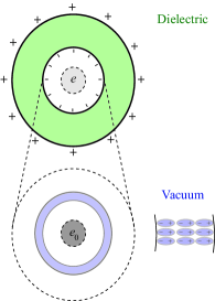
Figure 2: Screening in vacuum due to virtual particle-antiparticle pairs.

Running of $e^{2}/\varepsilon_{0}(k^{2})$ is in most ways equivalent to running of the square of effective charge in conventional QED,z but the physical interpretation is different. In a dielectric it is possible to have $\varepsilon_{0}<0,$ but $e_{\mathrm{eff}}^{2}<0$ makes no physical sense.

The simplest example of running coupling is a static charge, say $+e.$ In the Coulomb gauge $\mathbf{E}=-\nabla\Phi$ and $\omega=0$. Equation (10) with $k^{2}=-\mathbf{k}^{2}$ then gives

$$\Phi(\mathbf{k}^{2})=\frac{e}{\mathbf{k}^{2}\varepsilon_{0}(\mathbf{k}^{2})}\,.$$ (26)

In $\mathbf{r}$-space

$$\Phi(r)=\int\frac{d^{3}\mathbf{k}}{(2\pi)^{3}}\frac{e}{\mathbf{k}^{2}\varepsilon_{0}(\mathbf{k}^{2})}\exp(i\mathbf{k}\cdot\mathbf{r})\,.$$ (27)

This is equivalent to (7.93) in PS that is based on (2).

For electron-positron pairs alone $\Delta\Pi\ll 1$ so that $\varepsilon_{0}^{-1}\simeq(1+\Delta\Pi)/\varepsilon_{0}$ and LifshitzPitaevskii

$$\Phi(r)\simeq\frac{e}{4\pi\varepsilon_{0}r}\times\left\{\begin{array}[]{ll}1+\frac{2\alpha}{3\pi}\ln\left(\frac{\hbar}{m_{e}cr}\right)-\gamma-\frac{5}{6}&\qquad r\ll\hbar/m_{e}c,\\ &\\ 1+\frac{\alpha}{4\sqrt{\pi}}\frac{e^{-2m_{e}cr}/\hbar}{\left(m_{e}cr/\hbar\right)^{3/2}}&\qquad r\gg\hbar/m_{e}c,\end{array}\right.$$ (28)

where $m_{e}$ is the mass of the electron, $r$ is the distance from the fixed charge and $\gamma=0.577$ is Euler’s constant. The dielectric constant $\varepsilon_{0}$ decreases with increasing $\mathbf{k}^{2}$ or decreasing $r.$ For $r<\hbar/m_{e}c$ the Coulomb interaction becomes stronger as the charges approach each other.

References

- (1) P. W. Milonni, The Quantum Vacuum: An Introduction to Quantum Electrodynamics (Academic Press, New York, 1994)
- (2) L. Boi,The Quantum Vacuum: A Scientific and Philosophical Concept, from Electrodynamics to String Theory and the Geometry of the Microscopic World (John Hopkins University Press, Baltimore, 2011)
- (3) G. Leuchs, A. S. Villar and L. L. Sánchez-Soto, Appl. Phys. B 100, 9 (2010)
- (4) G. Leuchs and L. L. Sanchez-Soto, Eur. Phys. J. D 67, 57 (2013)
- (5) M. Urban, F. Couchot and X. Sarazin, Eur. Phys. J. D 67, 58 (2013)
- (6) S. A. R. Horsley and T. G. Philbin, New J. Phys. 16, 013030 (2014)
- (7) D. C. Kennedy and B. W. Lynn, Nucl. Phys. B 322, 1 (1989).
- (8) C. Itzykson and J. B. Zuber, Quantum Field Theory (Dover, New York, 1980)
- (9) M. E. Peskin and D. V. Schroeder, An Introduction to Quantum Field Theory (Addison-Wesley, Redwood City, CA, 1995)
- (10) L. D. Landau, in Niels Bohr and the Development of Physics, Edited by W. Pauli (Pergamon Press, London, 1955).
- (11) S. Weinberg, in Portrait of Gunnar Källén, Edited by C. Jarlskog (Springer, Berlin, 2013)
- (12) M. Göckeler, R. Horsley, V. Linke, P. Rakow, G. Schierholz and H. Stüben, Phys. Rev. Lett. 80, 4119 (1998)
- (13) Ya. B. Zel’dovich, ZhETF Pis’ma 6, 922 (1967)
- (14) K. G. Wilson Phys. Rev. B 4, 3174 (1971)
- (15) M. Binger and S. J. Brodsky, Phys. Rev. D 69, 095007 (2004)
- (16) L. I. Plimak and S. Stenholm, Ann. Phys. 327, 2691 (2012)
- (17) K. Gottfried and V. F. Weisskopf, Concepts of Particle Physics, Vol. II (Oxford University Press, 1986)
- (18) E. M. Lifshitz and L. P. Pitaevskii, Relativistic Quantum Theory, Part 2, Section 111 (Pergamon Press, NewYork, 1971)