Dimer geometry, amoebae and a vortex dimer model

Abstract

We present a geometrical approach and introduce a connection for dimer problems on bipartite and non-bipartite graphs. In the bipartite case the connection is flat but has non-trivial ${\bf Z}_{2}$ holonomy round certain curves. This holonomy has the universality property that it does not change as the number of vertices in the fundamental domain of the graph is increased. It is argued that the K-theory of the torus, with or without punctures, is the appropriate underlying invariant. In the non-bipartite case the connection has non-zero curvature as well as non-zero Chern number. The curvature does not require the introduction of a magnetic field. The phase diagram of these models is captured by what is known as an amoeba. We introduce a dimer model with negative edge weights which correspond to vortices. The amoebae for various models are studied with particular emphasis on the case of negative edge weights. Vortices give rise to new kinds of amoebae with certain singular structures which we investigate. On the amoeba of the vortex full hexagonal lattice we find the partition function corresponds to that of a massless Dirac doublet.

I Introduction

The subject of dimers has a large literature and has attracted the interest of both mathematicians and physicists. A few useful mathematical and physical sources are OkounkovKenyonSheffield ; OkounkovKenyon2006 ; CimasoniReshetikhin_I ; CimasoniReshetikhin_II ; Broomhead:2012 and Kasteleyn:1963 ; Fisher:1966 ; Nagle1989 ; Hanany-Kennaway:2005 ; Franco-et-al:2006 ; Hanany-Kennaway:2005 ; Feng-et-al:2008 ; OkounkovReshetikhinVafa:2006 ; Dijgraaf:2009 respectively, as well as references therein.

Dimer partition functions can be expressed as a sum of Pfaffians of a Kasteleyn matrix, $K$, which is a signed weighted adjacency matrix. The dimer partition function, with uniform weights, counts the number of perfect matchings of a graph. The model is naturally considered with positive weights and can have a non-trivial phase diagram as the weights are altered. In particular, it has a gapless phase which is described by the amoeba of a certain curve known as the spectral curve OkounkovKenyonSheffield ; OkounkovKenyon2006 (see section III). The Kasteleyn matrix can be thought of as a discrete lattice Dirac operator CimasoniReshetikhin_I ; CimasoniReshetikhin_II ; Nash_OConnor_jphysa:2009 and the finite size corrections to the partition function in the scaling limit coincide with that of a continuum Dirac–Fermion on a torus Nash_OConnor_jphysa:2009 . If one further adds signs to the weights the model describes a lattice Dirac operator in a fixed ${\bf Z}_{2}$ gauge field background. The presence of additional signs we refer to as the presence of vortices in the dimer system.

We review the basic construction of dimer models and give a detailed construction of the connection on the determinant line bundle over the positive frequency eigenvector space of the Kasteleyn matrix. We find that

• In the bipartite case the determinant line bundle has a flat connection.

• The flat connection has non-trivial ${\bf Z_{2}}$ holonomy in accordance with the $\widetilde{K}O$-theory of the torus.

• When vortices are included the system can describe additional massless Fermions and we present an example where the partition function, in the vortex full case of a hexagonal lattice, corresponds to a massless Dirac Fermion doublet.

• For certain vortex configurations, the domain where the system describes a massless Dirac operator, the amoeba can develop a pinch.

• The presence of vortices alters the thermodynamic phases, we exhibit a case where the gapped phase—an island, or compact oval in the amoeba corresponding to a massive Dirac phase—can, on introduction of vortices, shrink and even disappear.

The paper is organised as follows: section II describes basic results on dimers and dimer partition functions, focusing on bipartite dimer models. Sections III and IV describe a mathematical object known as an amoebae which describes the gapless parameter domain of the Kasteleyn matrix $K$. In section V we construct the vector bundle of positive eigenvalues of $iK$, and show that its determinant line bundle has a flat connection and in section VI we show that this connection has non-trivial ${\bf Z_{2}}$-holonomy in accordance with the $\widetilde{K}O$-theory of the punctured torus. Section VII treats dimers on non-bipartite graphs. Section VIII is devoted to dimer models in to the presence of vortices. In section IX we present our conclusions; this is followed by an appendix on some of the relevant K-theory.

II Dimers

Dimer models are concerned with the set of vertex matchings of a graph, or lattice, $\Gamma$. We shall consider $\Gamma$ to be a bipartite or non-bipartite lattice with $2n$ sites, or vertices, on the two torus $T^{2}$. A perfect matching, $m$, on $\Gamma$ is a disjoint collection of edges that contains all the vertices: for $m$ to exist $\Gamma$ must have an even number of vertices. An edge belonging to a matching is called a dimer and perfect matchings are the same thing as dimer configurations.

We denote the set of dimer configurations on $\Gamma$ by ${\cal M}(\Gamma)$. Then to each matching, $m\in{\cal M}(\Gamma)$, we assign a weight ${\rm e}^{-{\cal E}(m)}$; ${\cal E}(m)$ is normally required to be real in which case all weights are positive. We will find it useful to go beyond this restriction in the latter part of this paper and consider signed weights, but for the moment we take all weights to be positive.

Given this data the dimer partition function $Z(\Gamma)$ is given by:

$$Z(\Gamma)=\sum_{m\in{\cal M}(\Gamma)}{\rm e}^{-{\cal E}(m)}\,.$$ (1)

Each matching, $m$, consists of $n$ dimers with positive edge weights, $a_{e_{1}},\ldots,a_{e_{n}}$ whose relation to ${\cal E}(m)$ is that where $e_{i}$ are the edges of the matching $m$, and $a_{e_{i}}$ is the weight associated with the edge $e_{i}$, then

$${\rm e}^{-{\cal E}(m)}=\prod_{e_{i}\in m}a_{e_{i}}$$ (2)

yielding

$$Z(\Gamma)=\sum_{m\in{\cal M}(\Gamma)}\prod_{e_{i}\in m}a_{e_{i}}\,.$$ (3)

More generally one can consider $p$ dimers: i.e. $p$ matched edges where $p$ is less than or equal to the total number of edges; when $p=n$ one has a dimer model, otherwise one has a monomer-dimer system. Monomer-dimer systems have not yet yielded to exact solution methods.

An alternative generalisation is to consider some of the weights being negative, we will refer to such a system as containing vortices. It is relatively straightforward to solve for the partition function of such systems and as we shall see they have a rich physics. We shall only concern ourselves with dimer models, and dimer models with vortices, in this paper.

One can also investigate the probability of one, two, or more dimers (or edges), belonging to a matching $m$: to do this one uses, the characteristic function $\sigma_{e_{i}}$ of an edge $e_{i}$, and the dimer-dimer correlation functions $\left<\sigma_{e_{1}}\cdots\sigma_{e_{k}}\right>$: their joint definitions are that

$$\sigma_{e_{i}}(m) =\begin{cases}1&\text{if }e_{i}\in m\\ 0&\text{otherwise}\\ \end{cases}$$ (4)

$$\left<\sigma_{e_{1}}\cdots\sigma_{e_{k}}\right> =\frac{Z(e_{1},\ldots,e_{k};\Gamma)}{Z(\Gamma)}$$

$$\hbox{ with }\quad Z(e_{1},\ldots,e_{k};\Gamma) =\sum_{\left\{m\mid e_{1},\ldots e_{k}\in m\right\}}{\rm e}^{-{\cal E}(m)}\,.$$

For a planar region in ${\bf R}^{2}$, and a graph $\Gamma$ with $2n$ vertices, Kasteleyn Kasteleyn:1963 showed that

$$Z(\Gamma)=|\mbox{Pfaff}\,(K)|$$ (5)

where $\mbox{Pfaff}\,(K)$ is the Pfaffian of the Kasteleyn matrix $K$ which is a $2n\times 2n$ signed, antisymmetric, weighted adjacency matrix for $\Gamma$: Kasteleyn’s sign assignments in $K$ are precisely what is needed to convert $\mbox{Pfaff}\,(K)$ into the sum of positive terms that constitute the partition function $Z(\Gamma)$.

We specialise, for the moment, to the case where $\Gamma$ is bipartite, so that we can colour $n$ vertices black and the other $n$ white. This allows us to write $K$ in the form

$$K=\left(\begin{matrix}0&\hat{A}\\ -\hat{A}^{T}&0\\ \end{matrix}\right)$$ (6)

with $\hat{A}$ an $n\times n$ real matrix (we write $\hat{A}$ rather than $A$ since, later on, we want to use $A$ to denote a connection) and $T$ denotes transpose; note, too, that $\mbox{Pfaff}\,K=(-1)^{n(n-1)/2}\det\hat{A}$.

Let $V^{B}={\bf C}^{n}$ and $V^{W}={\bf C}^{n}$ be vector spaces generated by the sets of black and white vertices respectively, then $\hat{A}$ is the linear map

$$\hat{A}:V^{B}\longrightarrow V^{W}$$ (7)

defined by

$$\hat{A}_{ij}=\begin{cases}\epsilon_{ij}a_{ij}&\text{if $i$ is connected to $j$ by an edge with weight $a_{ij}$}\\ 0&\text{otherwise}\\ \end{cases}$$ (8)

where $\epsilon_{ij}=\pm 1$ is the sign associated to the edge whose weight is $a_{ij}$.

The signs $\epsilon_{ij}$ are computed by the clockwise odd rule Fisher:1966 : arrows are placed on the edges and $\epsilon_{ij}=+1$ when following an arrow and $-1$ when opposing one, and the product of the signs associated with any fundamental plaquette is $-1$ when the plaquette is circulated in an anticlockwise direction; such an assignment of signs is called a Kasteleyn orientation.

Note that all closed paths on bipartite graphs have an even number of edges: thus clockwise odd is also anticlockwise odd. This is false for non-bipartite graphs which, when Kasteleyn oriented, possess an orientation which can be detected—cf. below where we discuss Chern numbers.

The general result CimasoniReshetikhin_I ; CimasoniReshetikhin_II for a graph $\Gamma$ embedded in a closed oriented surface $\Sigma$ of genus $g$, is that the partition function of the dimer model on $\Gamma$ is given by

$$Z(\Gamma)=\frac{1}{2^{g}}\sum_{\vec{u}\in{\cal S}(\Sigma)}{\rm Arf}(\vec{u})\mbox{Pfaff}\,(K_{\vec{u}}(\Gamma))$$

where ${\cal S}(\Sigma)$ denotes the set of equivalence classes of the $2^{2g}$ spin structures on $\Sigma$, ${\rm Arf}(\vec{u})=\pm 1$ is the Arf-invariant of the spin structure labeled by $\vec{u}$, and $K_{\vec{u}}(\Gamma)$ is the Kasteleyn matrix with these boundary conditions.

When the graph $\Gamma$ is on a torus $T^{2}$, the weighted sum is over the four different Kasteleyn matrices $K_{u,v}$ corresponding to the four choices of periodic and anti-periodic boundary conditions around the cycles of the torus and

$$K_{u,v}=\left(\begin{matrix}0&\hat{A}_{u,v}\\ -\hat{A}^{T}_{u,v}&0\\ \end{matrix}\right)\,.$$ (9)

Each term in the sum corresponds to one of the $4$ discrete spin structures of $\Gamma$ on $T^{2}$ and, writing $Z({\rm e}^{2\pi iu},\rm{e}^{2\pi iv})=\det\hat{A}_{u,v}$, one has

$$Z(\Gamma)=\frac{1}{2}\left\{Z(1,-1)+Z(-1,1)+Z(-1,-1)-Z(1,1)\right\}\,.$$ (10)

Note that since $\Gamma$ is on a torus it is doubly periodic and can be realised as a quotient: one has

$$\Gamma=\frac{\widetilde{\Gamma}}{{\bf Z}^{2}}$$ (11)

where $\widetilde{\Gamma}$ is the graph in the plane consisting of all possible translations by elements of ${\bf Z}^{2}$ of an appropriate fundamental domain contained in $\Gamma$. However, $\Gamma$ itself may be multiple copies of this fundamental domain where the weights are repeated as translates. Then, by Fourier transforming $K_{u,v}$ we obtain a matrix $K_{u,v}(z,w)$ with off-diagonal block $\hat{A}_{u,v}(z,w)$.

On the torus corresponding to the $N\times M$ translates of a fundamental tile, the spin structure decomposition for the partition function is given by

$$Z= {(-1)}^{NM(NM-1)/2}\frac{1}{2}\sum_{u,v=0}^{1/2}{\rm e}^{2\pi i(\frac{1}{2}+u+v+2uv)}\mbox{Pfaff}\,K_{u,v}$$ (12)

$$=\frac{1}{2}\sum_{u,v=0}^{1/2}{\rm e}^{2\pi i(\frac{1}{2}+u+v+2uv)}\det\hat{A}_{u,v}$$

The determinant of $\hat{A}_{u,v}$ results in a polynomial $\hat{P}(z,w)$ with

$$\det\hat{A}_{u,v} =\prod_{n=0}^{N-1}\prod_{m=0}^{M-1}\hat{P}({\rm e}^{-\frac{2\pi i(n+u)}{N}},{\rm e}^{\frac{2\pi i(m+v)}{M}})$$

$$\ .$$ (13)

A key property of the polynomial $\hat{P}$ is that it has a pair of zeros $(z_{0},w_{0})$, $(\bar{z}_{0},\bar{w}_{0})$ related by complex conjugation.

We now describe the construction of $\hat{P}(z,w)$. Let us label an arbitrary translated copy of the fundamental domain from which $\Gamma$ is built by $\Gamma^{I,J}$ with $I,J\in{\bf Z}$. Here $I>0$ denotes the number of horizontal translations to the right, and $I<0$ the number of translations to the left, the integer $J$ labels vertical translations in a similar way; the fundamental domain is $\Gamma^{0,0}$.

Thus one has

$$\Gamma=\bigcup_{I=0}^{N-1}\bigcup_{J=0}^{M-1}\Gamma^{I,J}\quad\hbox{while}\quad\widetilde{\Gamma}=\bigcup_{I,J\in{\bf Z}}\Gamma^{I,J}\,.$$ (14)

Now to each $\Gamma^{I,J}$ we associate the matrix $\hat{A}^{I,J}(z,w)$; so that, if $\epsilon_{ij}a_{ij}$ denotes the signed weight of an edge joining vertex $i$ to $j$, then we define

$$\hat{A}^{I,J}_{ij}(z,w)=\begin{cases}z^{I}w^{J}\sum_{edges}\epsilon_{ij}a_{ij}\quad+&z^{L}w^{M}\sum_{edges}\epsilon_{ij}a_{ij}\\ \text{(if edge lies in $\Gamma^{I,J}$) }&\text{(if edge crosses into an {\it adjacent} domain $\Gamma^{L,M}$)}\\ 0&\text{otherwise.}\\ \end{cases}$$ (15)

With this data the fundamental domain containing the basic graph is $\Gamma^{0,0}$ and we define $\hat{A}(z,w)$ by writing

$$\hat{A}(z,w)=\hat{A}^{0,0}(z,w)$$ (16)

so that $\hat{P}(z,w)=\det\hat{A}^{0,0}(z,w)$ then $\hat{P}(z,w)$ is a Laurent polynomial in $z$ and $w$ with real coefficients.

Note that if we defined $\hat{A}(z,w)$ using a domain other than the fundamental domain, e.g. if we wrote $\hat{A}(z,w)=\hat{A}^{I,J}(z,w)$ then $\hat{P}(z,w)$ would just be multiplied by a monomial in $z$ and $w$ and the formula for the partition function would still hold true.

Now both the infinite graph $\widetilde{\Gamma}$, and its bipartite black-white assignment, are translation invariant, and the decomposition

$$\widetilde{\Gamma}=\bigcup_{I,J\in{\bf Z}}\Gamma^{I,J}$$ (17)

can be viewed as an indexing of $\widetilde{\Gamma}$ by the characters $z^{I}w^{J}$ of the translation group ${\bf Z}^{2}$; in other words $K^{I,J}(z,w)$ is simply the Fourier transform of the Kasteleyn matrix $\widetilde{K}$ of $\widetilde{\Gamma}$.

A pair of examples illustrating the above process can be quite simply given: consider $\Gamma$ to be the graphs tiled by the fundamental domains of figure 1.

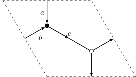
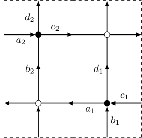
Figure 1: A hexagonal and a rectangular example

Then, for the hexagonal graph, we readily calculate that

$$K(z,w) =\left(\begin{matrix}0&c-b/z-aw\\ -(c-bz-a/w)&0\\ \end{matrix}\right)$$ (18)

$$\Rightarrow\hat{P}(z,w) =c-\frac{b}{z}-a\,w$$

while for the rectangular one we have

$$K(z,w) =\left(\begin{matrix}0&\hat{A}(z,w)\\ -\hat{A}^{T}(\bar{z},\bar{w})&0\\ \end{matrix}\right),\qquad\hat{A}(z,w)=\left(\begin{matrix}a_{1}-c_{1}z&d_{1}-b_{1}/w\\ -b_{2}+d_{2}w&c_{2}-a_{2}/z\\ \end{matrix}\right)$$ (19)

$$\Rightarrow\hat{P}(z,w) =a_{1}c_{2}+a_{2}c_{1}+b_{1}d_{2}+b_{2}d_{1}-\frac{a_{1}a_{2}}{z}-c_{1}c_{2}\,z-d_{1}d_{2}\,w-\frac{b_{1}b_{2}}{w}\,.$$

Observe that varying the dimer weights $a$ and $b$ in (18) is equivalent to moving $z$ and $w$ off the unit torus. In general, for any polynomial arising from a bipartite dimer construction, one can always absorb combinations of dimer weights into $z$ and $w$ to move them off the unit torus.

III Amoebae

Let $F(z,w)=\sum_{i,j}c_{ij}z^{i}w^{j}$ with $c_{ij},z,w\in{\bf C}$ be a polynomial, then its zero locus

$$F(z,w) =0$$ (20)

$$(z,w) \in({\bf C^{*}})^{2}$$

is a curve ${\cal C}$ in ${\bf C}^{2}$. The image of ${\cal C}$ in ${\bf R}^{2}$ under the logarithmic map ${\rm Ln}$ defined by

$${\rm Ln}:{\cal C}\longrightarrow{\bf R}^{2}$$ (21)

$$\qquad(z,w)\longmapsto(\ln|z|,\ln|w|)$$

is known as the amoeba ${\cal A(C)}$ of ${\cal C}$ so that ${\cal A(C)}={\rm Ln}({\cal C})$.

The polynomial $\hat{P}(z,w)$ above is a special case of such an $F(z,w)$ having real coefficients $c_{ij}$ and $\hat{P}(z,w)$ is central to much of what follows; its zero locus ${\cal C}$ is known as the spectral curve of the graph $\Gamma$.

The amoebae for the two graphs of figure 1 are displayed in figure 2; the closed curve in figure 2 (b) is called a compact oval—we have moved off the unit torus and used weights $a=|w|$, $b=1/|z|$, $c=1.2$ for figure 2 (a); and for example $a_{1}={\rm e}^{t}$, $a_{2}^{-1}=|z|{\rm e}^{t}$, $d_{1}=1/b_{2}=|w|$ with $\cosh(t)=2$ and all remaining weights unity for figure 2 (b).

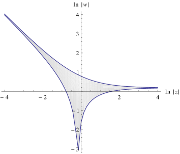
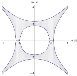
Figure 2: (a) Amoeba for $\hat{P}(z,w)=1.2-z^{-1}-w$ (b) Amoeba for $\hat{P}(z,w)=2+2\cosh(t)-z-z^{-1}-w-w^{-1}$,  $\cosh(t)=2$

Although an amoeba ${\cal A(C)}$ is unbounded in ${\bf R}^{2}$ it has finite area; in fact its area is bounded above by an irrational multiple of the area of the Newton polygon of $F(z,w)$—the Newton polygon $\Delta$ being the convex hull of the (integer) points $(i,j)\in{\bf R^{2}}$ for which $c_{ij}\not=0$. More precisely one has

$${\rm Area\,}({\cal A(C)})\leq\pi^{2}{\rm Area\,}(\Delta)\,.$$ (22)

After multiplication of $\hat{P}(z,w)$ by a suitable monomial to eliminate its negative powers, one obtains a polynomial $\widetilde{P}(z,w)$ of degree $d$, say. Since $\widetilde{P}(z,w)$ has real coefficients, it determines the real homogeneous polynomial $t^{d}\widetilde{P}(z/t,w/t)$ in $(z,w,t)$—where now $(z,w,t)\in{\bf R}^{3}$—and thus a real algebraic curve in ${\bf RP^{2}}$, this being natural geometrical data possessed by the spectral curve ${\cal C}$. We denote this real algebraic curve by $R{\cal C}$. When plotting the amoeba ${\cal A(C)}$ the signs of $z$ and $w$ play an essential role in determining all its components which, in turn, constitute the amoeba boundary.

For dimer models on bipartite graphs $R{\cal C}$ is a Harnack curve. Harnack curves are very special curves possessing the maximal number of components: i.e. $(d-1)(d-2)/2+1$. The integer $(d-1)(d-2)/2$ is the genus $g$ of the curve and is equal to the number of compact ovals of the amoeba.

It will be convenient for us to abuse terminology slightly and often refer to a curve ${\cal C}$ (rather than $R{\cal C}$) as being Harnack, the context should prevent any confusion.

A fundamental result of Kenyon, Okounkov, and Sheffield OkounkovKenyonSheffield and Kenyon and Okounkov OkounkovKenyon2006 is that every Harnack curve arises in this way so that the correspondence between the spectral curves of periodic hexagonal dimer models and Harnack curves is a bijection. Also all bipartite planar graphs can be realised inside a large enough hexagonal lattice by a combination of setting some dimer edge weights to zero and bond contraction Fisher:1966 ; OkounkovKenyon2006 ; thus no bipartite graph is excluded. In addition, the most general $d\times d$ hexagonal dimer model yields a generic Harnack curve of genus $(d-1)(d-2)/2$.

Positive rescaling of $z$ and $w$ gives a free action of ${\bf R^{+}}\times{\bf R^{+}}$ on the set ${\cal H}$ of Harnack curves; if one quotients ${\cal H}$ by this action one obtains what is called in OkounkovKenyon2006 the moduli space of Harnack curves. Amoebae provide natural coordinates for this moduli space: these coordinates being the areas of the holes and the distances between the tentacles OkounkovKenyon2006 .

When a curve ${\cal C}$ is Harnack the area of its amoeba is maximal and saturates the area inequality above—i.e.

$${\rm Area\,}({\cal A(C)})=\pi^{2}{\rm Area\,}(\Delta)$$ (23)

for ${\cal C}$ Harnack.

The converse of this equality also holds in the sense that ${\rm Area\,}({\cal A(C)})=\pi^{2}{\rm Area\,}(\Delta)$ implies that the curve ${\cal C}$ of $F(z,w)$ (after possible rescaling of $z$, $w$ and $F$ by complex constants) is invariant under complex conjugation and possesses a real part which determines a Harnack curve $R{\cal C}$ in ${\bf RP^{2}}$—cf. Mikhalkin_Rullgard2001 for more details.

Since the polynomial $\hat{P}(z,w)$ has real coefficients, the map ${\rm Ln}:{\cal C}\longrightarrow{\bf R}^{2}$ is generically, at least $2$ to $1$; however when ${\cal C}$ is Harnack ${\rm Ln}$ is $2$ to $1$ everywhere, except at real nodes which occur on the boundary of ${\cal A(C)}$, cf. OkounkovKenyon2006 ,Mikhalkin_Rullgard2001 . In addition $\hat{P}(z,w)$ has exactly two zeroes, $p=(z_{0},w_{0})$ and $\bar{p}=(\bar{z}_{0},\bar{w}_{0})$, on the unit torus $T^{2}$.

IV Phases and amoebae

The amoeba can be viewed as the massless or gapless phase with its bounding curves as the phase boundaries in a dimer model phase diagram OkounkovKenyonSheffield : the complement of the amoeba consists of both compact and non-compact regions. In the terminology of dimer models, as models of melting crystals, the non-compact regions exterior to the bounding ovals constitute the frozen regions. The amoeba itself is referred to as the liquid phase, and the interior of the compact ovals as the gaseous phase. There are also useful applications of these ideas to the Kitaev model Nash:2009prl and topological phase transitions Nash_OConnor_jphysa:2009 .

These different phases arise naturally when one calculates the correlation functions between the edges of $\Gamma$. The correlation functions possess three types of decay OkounkovKenyonSheffield —where a decay is measured by the fall off of $<\sigma_{e_{1}}\sigma_{e_{2}}>-<\sigma_{e_{1}}><\sigma_{e_{2}}>$ with distance between $e_{1}$ and $e_{2}$—these types being exponential, polynomial, or no decay, and they correspond to the gaseous, liquid and frozen phases respectively. In the context of Kasteleyn matrices as Dirac operators, the amoeba is the massless phase while the interiors of the compact ovals correspond to massive Dirac operators Nash_OConnor_jphysa:2009 .

V Dimer connections and curvatures

Now let $(z,w)=({\rm e}^{i\theta},{\rm e}^{i\phi})$ once again denote coordinates on $T^{2}$, rather than on ${\bf C^{2}}$, and let $\Gamma$ be a bipartite graph on $T^{2}$ whose Kasteleyn matrix $K$, when Fourier transformed, gives $K(z,w)$ where

$$K(z,w)=\left(\begin{matrix}0&\hat{A}(z,w)\\ -\hat{A}^{T}(\bar{z},\bar{w})&0\\ \end{matrix}\right)_{2n\times 2n}\,.$$ (24)

With these conventions the matrix $iK(z,w)$ is Hermitian. Here we use $2n$ for the number of vertices in the fundamental tile, in contrast to the usage in the introduction where $2n$ referred to the total number of vertices in the graph $\Gamma$.

If $\Gamma$ is non-bipartite its Kasteleyn matrix $K$ also has a Fourier transformed $(0,0)$ component $K(z,w)$ of the form

$$K(z,w)=\left(\begin{matrix}D_{1}(z,w)&\hat{A}(z,w)\\ -\hat{A}^{T}(\bar{z},\bar{w})&D_{2}(z,w)\\ \end{matrix}\right)_{2n\times 2n}$$ (25)

with at least one of the diagonal blocks $D_{1}(z,w)$ and $D_{2}(z,w)$ being non-zero and such that $iK(z,w)$ is still Hermitian.

We now describe how to use this data to construct a certain connection on $T^{2}$. The $n$-dimensional space of eigenvectors of $iK(z,w)$ with positive eigenvalues form a rank $n$ bundle over $T^{2}$ which we denote by $E^{+}$.

Let $x\in T^{2}$, then the fibre $E^{+}_{x}$, at $x$, has a basis consisting of the corresponding $n$ positive eigenvectors which we denote by

$$v_{1}(x),v_{2}(x),\ldots v_{n}(x)\,.$$ (26)

With respect to the standard complex inner product, fixed as $x$ varies, let each eigenvector $v_{i}(x)$ have unit norm and, in an orthonormal basis, have components $v_{ji},j=1,\ldots N$. When taken together the $v_{i}(x)$ form the non-square matrix $v(x)$ where

$$v(x)=\left(\begin{matrix}v_{11}(x)&\cdots&v_{1n}(x)\\ \vdots&\cdots&\vdots\\ v_{N1}(x)&\cdots&v_{Nn}(x)\\ \end{matrix}\right)_{N\times n}\qquad(N=2n)$$ (27)

giving one a map

$$v(x):{\bf C}^{n}\longrightarrow{\bf C}^{N}\,.$$ (28)

As $x$ varies the map $v(x)$ embeds the fibres $E^{+}_{x}$ of $E^{+}$—and thus the whole bundle—in the trivial bundle $T^{2}\times{\bf C}^{N}$; conversely, if $v^{*}(x)$ is the adjoint of $v(x)$, the map $P=v(x)v^{*}(x)$ is an orthogonal projection from ${\bf C}^{N}$ to ${\bf C}^{N}$ on which rests the non-triviality of $E^{+}$.

Summarising, and abbreviating $v(x)$ and $v^{*}(x)$ by $v$ and $v^{*}$ respectively, yields

$$\begin{aligned} v&=\left(\begin{matrix}v_{11}(x)&\cdots&v_{1n}(x)\\ \vdots&\cdots&\vdots\\ v_{N1}(x)&\cdots&v_{Nn}(x)\\ \end{matrix}\right)_{N\times n}\\ &\\ P&=vv^{*}\\ \end{aligned}\quad\begin{aligned} v^{*}&=\left(\begin{matrix}\bar{v}_{11}(x)&\cdots&\bar{v}_{1N}(x)\\ \vdots&\cdots&\vdots\\ \bar{v}_{n1}(x)&\cdots&\bar{v}_{nN}\\ \end{matrix}\right)_{n\times N}\\ &\\ v^{*}v&=I_{n\times n}\\ \end{aligned}\qquad(N=2n)$$ (29)

where $I_{n\times n}$ denotes the identity matrix on ${\bf C}^{n}$ and $P^{2}=P$; $v$ is called a partial isometry—it is not a real isometry since $v$ is not a square matrix.

A section $s$ of $E^{+}$ is then a map taking values in ${\bf C}^{N}$—i.e. one has

$$s:T^{2}\longrightarrow E^{+}_{x}\subset{\bf C}^{N}\,.$$ (30)

However, as usual, derivatives of $s$ such as $\partial_{\mu}s$ may not, as $x$ varies, still be $E^{+}_{x}$-valued, but we can project them back onto $E^{+}$ to take care of this problem thereby creating a covariant derivative on $E^{+}$. Thus the covariant derivative of $s$ is $\nabla_{\mu}s$ where

$$\nabla_{\mu}s=P\,\partial_{\mu}s\,.$$ (31)

Our choice of inner product above means that $\nabla_{\mu}$ is the covariant derivative corresponding to a $U(n)$ connection $A=A_{\mu}dx^{\mu}$, say, which we can identify by direct calculation as follows: if $f$ is a map

$$f:T^{2}\longrightarrow{\bf C}^{n}$$ (32)

then the product $vf$ gives us the section

$$T^{2}\xrightarrow{\;f\;}{\bf C}^{n}\xrightarrow{\;v\;}{\bf C}^{N}$$ (33)

and the covariant derivative formula gives

$$\nabla(vf) =Pd(vf)$$ (34)

$$=vv^{*}d(vf)$$

$$=vv^{*}\left\{dvf+vdf\right\}$$

$$=vdf+vv^{*}dvf$$

$$=v\left(df+Af\right),\quad\hbox{where }\quad A=v^{*}dv$$

$$=\nabla(vf),\qquad\quad\;\;\hbox{with }\quad\;\;\nabla=v(d+A)v^{*}$$

Hence the connection is the $U(n)$ matrix $A$ where

$$A=v^{*}dv$$ (35)

and its curvature is

$$dA+A\wedge A=dv^{*}\wedge dv+v^{*}dv\wedge v^{*}dv$$ (36)

So the covariant derivative and curvature on $E^{+}$ are $\nabla$ and $F$ respectively, with $F=\nabla^{2}=v(dA+A\wedge A)v^{*}$. A routine calculation shows that

$$F=P\,dP\wedge dPP$$ (37)

We shall examine the connection and its curvature in the subsequent sections but note that its introduction has not required the presence of a magnetic field.

VI Holonomy and Flat connections

We will be interested in the $U(1)$ connection associated with $tr(F)$ as it is this that gives the first Chern class of the connection. It turns out that for bipartite graphs the curvature $tr(F)$ is zero so that the associated $U(1)$ connection is flat: nevertheless this connection is non-trivial as it has non-trivial holonomy as we shall now show.

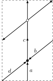
Figure 3: A bipartite graph with $\hat{P}(z,w)=c-b\,z-\frac{a}{w}-\frac{d}{wz}$

It is instructive to first study a case where $n=1$ and we do this for the graph $\Gamma$ shown in figure 3. For the bipartite case, when $D_{1}=D_{2}=0$, one punctures the torus $T^{2}$ at the points $p$ and $\bar{p}$ since $\hat{P}(z,w)$ vanishes there, we denote the punctured torus by $T^{2}_{p,\bar{p}}$. One finds that the connection $A$ and its curvature $F$ are given by

$$A =\frac{1}{2}f^{-1}df,\quad\text{ with }\quad f=\sqrt{\frac{\hat{P}(z,w)}{\overline{\hat{P}(z,w)}}}$$ (38)

$$F =0$$

so that we have a flat connection; however the connection $A$ is not trivial as it has non-trivial holonomy $\exp\left[\int_{C}A\right]$ for some curves $C$ on $T^{2}_{p,\bar{p}}$. In other words for such curves

$$\exp\left[\int_{C}A\right] \not=1$$ (39)

$$\text{i.e.}\qquad\int_{C}\frac{A}{2\pi i} \not\in{\bf Z}$$

As an example, for figure 3 choose $a=b=c=d=1$ so that

$$\hat{P}(z,w)=1-\frac{1}{w}-z-\frac{1}{wz}$$ (40)

and thus $\hat{P}(z,w)=0$ at the points

$$p=({\rm e}^{i\pi/2},1),\qquad\bar{p}=({\rm e}^{-i\pi/2},1)$$ (41)

One then immediately discovers by direct calculation that if $C$ is a small circle

$$\int_{C}\,\frac{A}{2\pi i}=\begin{cases}\;\;\;\frac{1}{2}&\text{if $C$ encircles $p$ but not $\bar{p}$}\\ -\frac{1}{2}&\text{if $C$ encircles $\bar{p}$ but not $p$}\\ \end{cases}$$ (42)

Hence we obtain non-trivial holonomy and it is easy to choose a different $C$ and obtain other results: indeed if $C$ does not contain $p$ or $\bar{p}$, but is non-contractible because it is a non-trivial homology cycle, then $\exp\left[\int_{C}A\right]$ can also have non-trivial holonomy.

For example if $C$ is the curve $\theta=\theta_{0}$, $\theta_{0}$ constant, then

$$\int_{C}\frac{A}{2\pi i}=\left\{\begin{matrix}-\frac{1}{2}&\text{if $\theta_{0}\in\left(-\frac{\pi}{2},\frac{\pi}{2}\right)$}\\ &\\ \quad 0&\text{otherwise}\\ \end{matrix}\right.$$ (43)

Non-trivial flat connections require $T^{2}_{p,\bar{p}}$ to have a non vanishing fundamental group but one knows that $T^{2}_{p,\bar{p}}$ is homotopic to a bouquet of three circles (meaning three circles sharing one common point) and therefore

$$\pi_{1}(T^{2}_{p,\bar{p}})={\bf Z}*{\bf Z}*{\bf Z}\quad\left(\text{the free group on three generators}\right)$$ (44)

so all is satisfactory.

These properties of flatness and non-trivial holonomy persist—for the appropriate curvature and connection—when the bipartite graph is enlarged as we now demonstrate.

First let $F$ be the curvature coming from the Kasteleyn matrix $K(z,w)$ for a general bipartite graph. One has

$$K(z,w)=\left(\begin{matrix}0&\hat{A}(z,w)\\ -\hat{A}(\bar{z},\bar{w})&0\\ \end{matrix}\right)_{2n\times 2n}$$ (45)

with curvature $F=PdP\wedge dPP$ then it is easy to see that

$$\;\mbox{tr}\;(F)=0\,.$$ (46)

For, abbreviating $\hat{A}(\bar{z},\bar{w})$ to $\hat{A}^{*}$, and setting $Q=(\hat{A}\hat{A}^{*})^{-1/2}\hat{A}$, $P$ can be written as

$$P=\frac{1}{2}\left(\begin{matrix}I&iQ\\ -iQ^{*}&I\\ \end{matrix}\right)_{2n\times 2n}$$ (47)

with $I$ the $n\times n$ identity matrix. Hence

$$dP =\frac{1}{2}\left(\begin{matrix}0&idQ\\ -idQ^{*}&0\\ \end{matrix}\right)$$ (48)

$$\Rightarrow dP\wedge dP =\frac{1}{2^{2}}\left(\begin{matrix}dQ\wedge dQ^{*}&0\\ 0&dQ^{*}\wedge dQ\\ \end{matrix}\right)$$

and so we have,

$$\;\mbox{tr}\;(F) =\;\mbox{tr}\;(PdP\wedge dPP)=\;\mbox{tr}\;(PdP\wedge dP)$$ (49)

$$=\frac{1}{2^{3}}\;\mbox{tr}\;\left\{\left(\begin{matrix}I&iQ\\ -iQ^{*}&I\\ \end{matrix}\right)\left(\begin{matrix}dQ\wedge dQ^{*}&0\\ 0&dQ^{*}\wedge dQ\\ \end{matrix}\right)\right\}$$

$$=\frac{1}{2^{3}}\;\mbox{tr}\;\left(\begin{matrix}dQ\wedge dQ^{*}&-iQdQ^{*}\wedge dQ\\ iQ^{*}dQ\wedge dQ^{*}&dQ^{*}\wedge dQ\\ \end{matrix}\right)$$

$$=\frac{1}{2^{3}}\left\{\;\mbox{tr}\;\left(dQ\wedge dQ^{*}\right)+\;\mbox{tr}\;\left(dQ^{*}\wedge dQ\right)\right\}$$

$$=0$$

as claimed.

Now, just as when $n=1$, there is non-trivial holonomy when $n>1$: we shall also find the interesting result that the holonomy obtained is universal and is independent of $n$.

However first we must identify an appropriate line bundle $L\subset E^{+}$ with connection and to this end we shall use the following notation: we denote the connection and curvature on any bundle $E$ by $F^{E}$ and $A^{E}$ respectively.

So taking our bundle $E^{+}$—whose connection and curvature were formerly denoted by $A$ and $F$ above—we now denote these quantities by

$$A^{E^{+}}$$ (50)

and $F^{E^{+}}$ respectively. As we will see below, the line bundle $L$ that we seek is simply the determinant line bundle of $E^{+}$, that is

$$L=\det(E^{+})$$ (51)

Let $v_{+}^{1},v_{+}^{2}\cdots v^{n}_{+}$ denote the $n$ unit normalised positive eigenvectors of $iK(z,w)$, then this bundle has projection $P_{\det(E^{+})}$ where

$$P_{\det(E^{+})} =V_{\det(E^{+})}V^{*}_{\det(E^{+})}$$ (52)

$$\text{ with}\qquad V_{\det(E^{+})} =v^{1}_{+}\wedge v^{2}_{+}\wedge\cdots\wedge v^{n}_{+}$$

and the associated connection is therefore $A^{\det(E^{+})}$ where

$$A^{\det(E^{+})} =V_{\det(E^{+})}^{*}dV_{\det(E^{+})}$$ (53)

$$=\left<v^{1}_{+}\wedge v^{2}_{+}\wedge\cdots\wedge v^{n}_{+},d(v^{1}_{+}\wedge v^{2}_{+}\wedge\cdots\wedge v^{n}_{+})\right>$$

Here it may be useful to recall that, if $W$ is a vector space, the inner product on $\Lambda^{n}W$, which for orthonormal ${\bf e_{i}}\in W$ renders the vectors ${\bf e_{i_{1}}}\wedge{\bf e_{i_{2}}}\wedge\cdots\wedge{\bf e_{i_{n}}}$ orthonormal, is given by

$$<a_{1}\wedge a_{2}\cdots\wedge a_{n},b_{1}\wedge b_{2}\cdots\wedge b_{n}>=\det(M(a,b))$$ (54)

$$M(a,b)=\left(\begin{matrix}<a_{1},b_{1}>&\cdots&<a_{1},b_{n}>\\ <a_{2},b_{1}>&\cdots&<a_{2},b_{n}>\\ \vdots&\ddots&\vdots\\ <a_{n},b_{1}>&\cdots&<a_{n},b_{n}>\\ \end{matrix}\right)$$

In fact,

$$A^{\det(E^{+})}=\;\mbox{tr}\;(A^{E^{+}})$$ (55)

To see this note first that

$$A^{\det(E^{+})} =<v_{+}^{1},dv_{+}^{1}>+\cdots+<v_{+}^{n},dv_{+}^{n}>$$ (56)

$$=(v_{+}^{1})^{*}dv_{+}^{1}+\cdots+(v_{+}^{n})^{*}dv_{+}^{n}$$

and for $E^{+}$ we observe that $v_{+}^{i}$ is a $2n\times 1$ column vector and $(v_{+}^{i})^{*}$ is a $1\times 2n$ row vector with

$$V_{E^{+}} =\left(\begin{matrix}v_{+}^{1}&v_{+}^{2}&\cdots&v_{+}^{n}\\ \end{matrix}\right)_{2n\times n}$$ (57)

$$V^{*}_{E^{+}} =\left(\begin{matrix}(v_{+}^{1})^{*}\\ (v_{+}^{2})^{*}\\ \vdots\\ (v_{+}^{n})^{*}\\ \end{matrix}\right)_{n\times 2n}$$

where $V^{*}_{E^{+}}V_{E^{+}}=I_{n\times n}$ and the projection $P_{E^{+}}$ is given by $P_{E^{+}}=V_{E^{+}}V^{*}_{E^{+}}$. Hence

$$A^{E^{+}}=V^{*}_{E^{+}}dV_{E^{+}}=\left(\begin{matrix}(v_{+}^{1})^{*}dv_{+}^{1}&\cdots&(v_{+}^{1})^{*}dv_{+}^{n}\\ \vdots&\cdots&\vdots\\ (v_{+}^{n})^{*}dv_{+}^{1}&\cdots&(v_{+}^{n})^{*}dv_{+}^{n}\\ \end{matrix}\right)$$ (58)

yielding

$$\;\mbox{tr}\;(A^{E^{+}})=(v_{+}^{1})^{*}dv_{+}^{1}+(v_{+}^{2})^{*}dv_{+}^{2}+\cdots+(v_{+}^{n})^{*}dv_{+}^{n}$$ (59)

as claimed.

One can check that $A^{\det(E^{+})}=\;\mbox{tr}\;(A^{E^{+}})$ is indeed a $U(1)$ connection; it is also flat since its curvature $F^{\det(E^{+})}$ satisfies

$$F^{\det(E^{+})} =d\;\mbox{tr}\;(A^{E^{+}})$$ (60)

$$=\;\mbox{tr}\;(d_{A}A^{E^{+}})=\;\mbox{tr}\;(F^{E^{+}})$$

$$=0$$

Now we are ready to calculate the holonomy of $A^{\det(E^{+})}$ round some curve $C$: let

$$K=\left(\begin{matrix}0&\hat{A}\\ -\hat{A}^{*}&0\\ \end{matrix}\right)$$ (61)

and $u_{+}$ satisfy

$$\hat{A}^{*}\hat{A}u_{+}=\lambda_{+}u_{+},\qquad\left\langle u_{+},u_{+}\right\rangle=1$$ (62)

then $v_{+}$ is a unit norm eigenvector of $iK$ with eigenvalue $\sqrt{\lambda_{+}}$ where

$$v_{+}=\frac{1}{\sqrt{2}}\left(\begin{matrix}\textstyle w_{+}\\ {\textstyle-iu_{+}}\\ \end{matrix}\right),\qquad w_{+}=\frac{\hat{A}u_{+}}{\sqrt{\lambda^{i}_{+}}}$$ (63)

Using this orthogonal decomposition for each $v_{+}^{i}$ we calculate that

$$\left<v^{1}_{+}\wedge v^{2}_{+}\wedge\cdots\wedge v^{n}_{+},d(v^{1}_{+}\wedge v^{2}_{+}\wedge\cdots\wedge v^{n}_{+})\right> =\frac{1}{2}\left\{(u_{+}^{1})^{*}du_{+}^{1}+\cdots+(u_{+}^{n})^{*}du_{+}^{n}\right.$$ (64)

$$\left.\quad+(w_{+}^{1})^{*}dw_{+}^{1}+\cdots+(w_{+}^{n})^{*}dw_{+}^{n}\right\}$$

$$= \frac{1}{2}\left\{\left<w^{1}_{+}\wedge w^{2}_{+}\wedge\cdots\wedge w^{n}_{+},d(w^{1}_{+}\wedge w^{2}_{+}\wedge\cdots\wedge w^{n}_{+})\right>\right.$$

$$\;\;+\left.\left<u^{1}_{+}\wedge u^{2}_{+}\wedge\cdots\wedge u^{n}_{+},d(u^{1}_{+}\wedge u^{2}_{+}\wedge\cdots\wedge u^{n}_{+})\right>\right\}$$

But now take note that

$$w^{1}_{+}\wedge w^{2}_{+}\wedge\cdots\wedge w^{n}_{+} =\frac{\det(\hat{A})}{\sqrt{\lambda_{+}^{1}\lambda_{+}^{2}\cdots\lambda_{+}^{n}}}u^{1}_{+}\wedge u^{2}_{+}\wedge\cdots\wedge u^{n}_{+}$$ (65)

$$=f(z,w)\,u^{1}_{+}\wedge u^{2}_{+}\wedge\cdots\wedge u^{n}_{+},\quad\hbox{ where }f(z,w)=\sqrt{\frac{\hat{P}(z,w)}{\overline{\hat{P}(z,w)}}}$$

and hence we obtain

$$A^{\det(E^{+})}=\frac{1}{2}f^{-1}df+(u_{+}^{1})^{*}du_{+}^{1}+\cdots+(u_{+}^{n})^{*}du_{+}^{n}$$ (66)

Thus our formula for the holonomy of $A^{\det(E^{+})}$ round a curve $C$ on the torus $(z,w)=({\rm e}^{i\theta},{\rm e}^{i\phi})$ is

$$\int_{C}A^{\det(E^{+})}=\frac{1}{2}\int_{C}f^{-1}df+\int_{C}(u_{+}^{1})^{*}du_{+}^{1}+\cdots+\int_{C}(u_{+}^{n})^{*}du_{+}^{n}$$ (67)

Now let us take a basis for the $n$ dimensional space on which $\hat{A}^{*}\hat{A}$ acts in which $u_{+}^{i}$ takes the form

$$u_{+}^{i}=\left(\begin{matrix}0\\ \vdots\\ {\rm e}^{i\psi_{i}}\\ \vdots\\ 0\\ \end{matrix}\right)_{n\times 1}\qquad\begin{matrix}\psi_{i}\equiv\psi_{i}(\theta,\phi)\hfill\\ \psi_{i}(\theta,\phi)\hbox{ periodic in $\theta$ and $\phi$}\\ \end{matrix}$$ (68)

where the only non-zero entry in the representation of $u_{+}^{i}$ above is $\psi_{i}$ which occupies the $i^{th}$ position. This means that

$$\frac{1}{2\pi i}\int_{C}(u_{+}^{i})^{*}du_{+}^{i}\in{\bf Z}$$ (69)

for each $i$. One can now easily check that

$$\frac{1}{2\pi i}\int_{C}A^{\det(E^{+})}=\frac{1}{2}+k,\,k\in{\bf Z}\text{$\quad$ if $C$ contains one of the zeroes of $\hat{P}(z,w)$ }$$ (70)

The holonomies for other choices of $C$ can also be readily verified.

Thus the only non-trivial contribution to the holonomy group element comes from the term ${1/2}\int_{C}f^{-1}df$ which is precisely the term obtained in the two site case: we have therefore deduced that

$$\exp\left[\int_{C}A^{\det(E^{+})}\right]=\exp\left[\frac{1}{2}\int_{C}f^{-1}df\right]$$ (71)

Hence, as claimed above, we have shown that, when we have $2n$ sites, the holonomy of the connection $A^{\det(E^{+})}$ is a universal invariant independent of $n$. Notice that if the $\frac{1}{2}$ in (71) is replaced by $1$ the holonomy becomes trivial. This is precisely what occurs if we consider the matrix direct sum of $K$ with itself, $K\oplus K$, whose bundle of positive eigenvectors is $E^{+}\oplus E^{+}$ where, following (66), we find that

$$\exp\left[\int_{C}A^{\det(E^{+}\oplus E^{+})}\right]=\exp\left[\int_{C}f^{-1}df\right]=1$$ (72)

and the holonomy is trivial. This latter ${\bf Z_{2}}$ observation is a $\widetilde{K}O$-theory one, see the appendix.

Passing to the underlying real bundles, the real K-theory of $T^{2}_{p,\bar{p}}$—cf. the appendix—is given by

$$\widetilde{K}O(T^{2}_{p,\bar{p}})={\bf Z_{2}}\oplus{\bf Z_{2}}\oplus{\bf Z_{2}}$$ (73)

and this captures the ${\bf Z_{2}}$-Fermionic nature of the holonomy for bundles of any rank. We further note that were we to perform the same computation as above for the continuum massless Dirac operator on the plane we would also find that the associated connection had ${\bf Z_{2}}$ holonomy. The relation with $\widetilde{K}O$ theory can be understood in a similar manner, since, topologically, the punctured plane is $S^{2}_{p,q}$, the twice punctured sphere, and from the appendix we can deduce that $\widetilde{K}O(S^{2}_{p,q})={\bf Z_{2}}$. One can conclude that it is the Fermionic nature of the dimer system that is responsible for this topological observation.

VII Non-bipartite graphs and Chern numbers

Now we come to cases where the curvature is non-zero: this happens for non-bipartite graphs. Such a case occurs when, for example, two non-bipartite edges are added to the graph of figure 3. We display the resulting graph $\Gamma$ in figure 4.

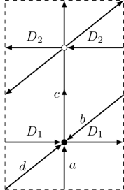
Figure 4: A non-bipartite graph whose associated curvature is non-zero.

The Kasteleyn matrix $K(z,w)$ of this $\Gamma$ is given by

$$K(z,w) =\left(\begin{matrix}D_{1}(z-\bar{z})&\hat{P}(z,w)\\ -\hat{P}(\bar{z},\bar{w})&-D_{2}(z-\bar{z})\\ \end{matrix}\right)$$ (74)

$$\text{with }\qquad\qquad\quad\hat{P}(z,w) =c-b\,z-\frac{a}{w}-\frac{d}{wz},\;D_{1},D_{2}\text{ constants}$$

We decompose $K(z,w)$ using the three Pauli matrices $\sigma_{1},\sigma_{2},\sigma_{3}$ and the identity, $I$, which, for convenience, we denote by $\sigma_{0}$. This yields

$$iK(z,w) =m_{0}\,\sigma_{0}+m_{1}\,\sigma_{1}+m_{2}\,\sigma_{2}+m_{3}\,\sigma_{3}$$ (75)

$$=\left(\begin{matrix}m_{0}+m_{3}&m_{1}-im_{2}\\ m_{1}+im_{2}&m_{0}-m_{3}\\ \end{matrix}\right),\quad(m_{\mu}=\frac{i}{2}\;\mbox{tr}\;(K(z,w)\,\sigma_{\mu}),\;\mu=0,\ldots,3)$$

and, for the two eigenvectors $v_{\pm}$, with eigenvalue $\lambda_{\pm}$, we have

$$v_{\pm}=\frac{\textstyle 1}{\textstyle\sqrt{2m(m\mp m_{3})}}\left(\begin{matrix}m_{1}-im_{2}\\ \pm m-m_{3}\\ \end{matrix}\right),\quad\lambda_{\pm}=m_{0}\pm m,\quad m=\sqrt{m_{1}^{2}+m_{2}^{2}+m_{3}^{2}}\,.$$ (76)

The curvatures $F$ of $v_{+}$ is given by

$$F=\frac{i}{4}\epsilon_{ijk}\frac{m_{i}dm_{j}dm_{k}}{m^{3}}$$ (77)

which we note vanishes for the bipartite case where $m_{3}=0$.

Note that in this non-bipartite case where $m_{3}\not=0$, the points $p,\bar{p}\in T_{2}$ are now no longer excluded since $\lambda_{+}$ is positive there; thus the bundle $E^{+}$ now extends over all of $T_{2}$. Let $c_{1}(E^{+})$ denote the value of the first Chern class on $E^{+}$ so that (some authors define $c_{1}(E^{+})$ with the opposite sign to ours)

$$c_{1}(E^{+})=\int_{T^{2}}\frac{iF}{2\pi}$$ (78)

In order to conveniently display the values of the edge weights we shall denote $c_{1}(E^{+})$ by $c_{1}(a,b,c,d,D_{1},D_{2})$, in an obvious notation. Some selected results for $c_{1}(a,b,c,d,D_{1},D_{2})$ are that

$$\ c_{1}(1,1,1,1,1,1)=-1$$ (79)

$$c_{1}(1.1,1.2,1.3,1,1,1)=-1$$    (topological invariance)

other non-zero values are easily calculated. The value of $c_{1}(a,b,c,d,D_{1},D_{2})$ is stable under small changes in the edge weights; and when $c_{1}(E^{+})\not=0$ it provides a certain topological stability to the dimer configuration.

Note that changing the Kasteleyn orientation reverses the sign of the diagonal terms in $K(z,w)$ and changes the sign of $c_{1}(a,b,c,d,D_{1},D_{2})$. A non-zero Chern number therefore distinguishes between clockwise odd and anti-clockwise odd Kasteleyn orientation.

We already know that when the graph is bipartite e.g., when $D_{1}=D_{2}=0$ the curvature $F$ and, hence the Chern number, both vanish. However the Chern number can also vanish in the non-bipartite case when the edge weights are such that $m_{1}-im_{2}\neq 0$ for any point on the unit torus $T^{2}$, i.e. the edge weights specify a point off the associated bipartite amoebae.

For suppose that

$$c>a+b+d$$ (80)

so that one is off the amoeba of $\hat{P}(z,w)$, then even when $D_{1},D_{2}\not=0$, one has $c_{1}(a,b,c,d,D_{1},D_{2})=0$. For example, setting $c=3.2$ and all other weights to unity yields

$$c_{1}(3.2,1,1,1,1,1)=0$$ (81)

In fact this is a natural result as the line bundle $E^{+}$ has a global non vanishing section $s$ given by

$$s =\left<v,v\right>,\quad v=\left(\begin{matrix}m_{1}-im_{2}\\ m-m_{3}\\ \end{matrix}\right)$$ (82)

$$=2m(m-m_{3})$$

so that $s$ cannot vanish, since

$$s=0\Rightarrow\begin{cases}m=m_{3}&\text{i.e. $\hat{P}(z,w)=0$ , impossible off the amoeba}\\ m=0&\text{i.e. $m_{3}=\hat{P}(z,w)=0$, also impossible}\\ \end{cases}$$ (83)

In general the curvature $F$ will be non-zero for non-bipartite graphs that have a subgraph on the bipartite amoeba. However, remember from (77) that

$$m_{3}=0\Rightarrow F=0$$ (84)

but

$$m_{3}=i(D_{1}+D_{2})(z-\bar{z})$$ (85)

so that $F=0$ when $D_{1}=-D_{2}$; the connection $A=v^{*}_{+}dv_{+}$ is then flat. This connection has non-trivial holonomy and so is not trivial: indeed if we choose the curve $C$ we had above, defined by $\theta=\theta_{0}$, $\theta_{0}$ constant, then with $c=a=b=d=1$

$$\exp\left[\int_{C}A\right]=\left\{\begin{matrix}-\frac{1}{2}&\text{if $\theta_{0}\in\left(-\frac{\pi}{2},\frac{\pi}{2}\right)$}\\ &\\ \quad 0&\text{otherwise}\\ \end{matrix}\right.$$ (86)

and so one has non-trivial holonomy as well as flatness.

Reversing the sign of one of $D_{1}$ and $D_{2}$ in (LABEL:nonbipartitetwosite) introduces vortices and makes the curvature $F$ of (77) zero.

However, reversing both $D_{1}$ and $D_{2}$ changes the sign of $F$. It reverses the Kasteleyn orientation of the graph but the partition function on the torus is unaffected. Hence the curvature, and Chern numbers are sensitive to the Kasteleyn orientation, though the partition function is not.

These results are naturally interpreted via the real and complex K-theory of $T^{2}$—cf. the appendix for more details. The K-theory statements for $T^{2}$ say that

$$\widetilde{K}(T^{2}) ={\bf Z}$$ (87)

$$\widetilde{K}O(T^{2}) ={\bf Z_{2}}\oplus{\bf Z_{2}}\oplus{\bf Z_{2}}$$

and this allows for both integer and ${\bf Z_{2}}$ invariants which is as one wants. Hence flat connections with non-trivial holonomy are not restricted to bipartite graphs; note that this example requires that one of the edge weights is negative so that, as discussed in the next section, a vortex is present.

VIII Non Harnack amoebae: singularities and area shrinking

Let us assume, for the moment, that our graphs $\Gamma$ are bipartite. If a plaquette of $\Gamma$ contains one or more negative edge weights, this can be compensated for by changing an arrow direction, then the clockwise odd rule will be violated for the plaquettes on either side of this link: this can be interpreted as the presence of vortices on these plaquettes. The negative weight assignment means that the curve ${\cal C}$ is non-Harnack.

This can be detected in two equivalent ways:

1. The amoeba map

   $$Ln:{\cal C}\longrightarrow{\bf R}^{2},\quad\text{(complex double fold or pinch)}$$ (88)

   fails to be $2$ to $1$ for all points on the amoeba.

2. The amoeba satisfies

   $${\rm Area\,}({\cal A(C)})<\pi^{2}{\rm Area\,}(\Delta)\quad\text{(Area shrinking)}$$ (89)

   where $\Delta$ is the Newton polygon of ${\cal C}$.

We shall now give some concrete examples of these phenomena.

Example A complex double fold

For our first example we take the graph shown in figure 5 below. Now, moving $z$ and $w$ off the unit torus and setting all edge weights to unity, except for $J_{1z}$, which is set equal to $J$; the resulting $K(z,w)$ is given by

Figure 5: A hexagonal chain of length $n$

$$K(z,w)=\left(\begin{matrix}0&\hat{A}(z,w)\\ -\hat{A}^{T}(\bar{z},\bar{w})&0\\ \end{matrix}\right)_{2n\times 2n}$$ (90)

and

$$\hat{A}(z,w)=\left(\begin{matrix}1-Jw&0&\cdots&0&-\frac{1}{z}\\ -1&1-w&0&\cdots&0\\ 0&-1&1-w&\cdots&0\\ \vdots&\vdots&\vdots&\ddots&\vdots\\ 0&\cdots&0&-1&1-w\\ \end{matrix}\right)_{n\times n}$$ (91)

which yields

$$\hat{P}(z,w)=(1-Jw)(1-w)^{n-1}-\frac{1}{z},\;n=2,\ldots\quad.$$ (92)

We are interested in what happens when the edge weight $J<0$. We do not consider the case $n=1$ as this gives the hexagonal graph of figure 1 and does not yield a vortex when $J<0$: changing the sign of $J$ in this case gives an alternative Kasteleyn orientation of the graph; the orientation is still clockwise odd and ${\cal C}$ is still Harnack.

However when $n\geq 2$ and $J<0$ we get two adjacent vertical columns of vortex filled plaquettes followed by $n-2$ non-vortex columns in a periodic structure and we shall find that the $2$ to $1$ property of the map ${\rm Ln}:{\cal C}\longrightarrow{\bf R}^{2}$ fails.

Now we set $J=-1$ and turn first to the case $n=2$, in which case all plaquettes on the lattice contain a vortex. We have

$$\hat{P}(z,w)=1-w^{2}-\frac{1}{z}$$ (93)

and it is easy to check directly—or by comparison with the amoeba of $\hat{P}(z,w)=1-w-1/z$—that ${\rm Ln}$ is now $4$ to $1$ everywhere and $2$ to $1$ nowhere. One can also easily check that the area of the amoeba for $J=1$ is $\pi^{2}$, as required by the Harnack condition, while for $J=-1$ it is $\pi^{2}/2$.

We show the amoeba—together with that of $\hat{P}(z,w)=1-w-1/z$—in figure 6; the dark shading denotes the $4$ to $1$ region for ${\rm Ln}$.

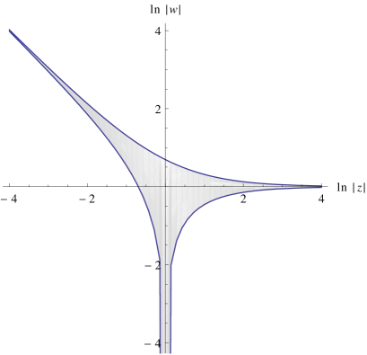
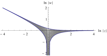
Figure 6: The amoebae for $\hat{P}(z,w)=1-w-1/z$ and $\hat{P}(z,w)=1-w^{2}-1/z$. In the first figure ${\rm Ln}$ is $2$ to $1$ everywhere while in the second figure it is $4$ to $1$ everywhere.

For the remaining values, $n\geq 3$, the amoeba ${\cal A(C)}$ has both a $2$ to $1$ region and a $4$ to $1$ region; the two regions being separated by a complex double folding (Mikhalkin Mikhalkinsingularities ). We proceed to find the singularity of ${\rm Ln}$.

Quite generally a singularity occurs when the Jacobian ${\rm J(Ln})$ fails to have maximal rank everywhere on ${\cal A(C)}$. For the amoeba we have

$$\begin{aligned} &{\rm Ln}:{\cal C}\longrightarrow{\bf R}^{2}\\ &\left(f(w),w\right)\longmapsto\left(\ln\left|f(w)\right|,\ln|w|\right)\\ \end{aligned}\quad\hbox{ where }\quad f(w)=\frac{1}{(1-Jw)(1-w)^{n-1}}$$ (94)

and our singularity condition is therefore

$$\det({\rm J(Ln)})=0$$ (95)

where, if $w=\rho{\rm e}^{i\phi}$, one has

$${\rm J(Ln)}=\left(\begin{matrix}\partial_{\rho}\ln|f|&\partial_{\rho}\ln|w|\\ \partial_{\phi}\ln|f|&\partial_{\phi}\ln|w|\\ \end{matrix}\right)\,.$$ (96)

We see then that the amoeba is singular where

$$\partial_{\phi}\ln|f|=0\,.$$ (97)

Writing $\rho={\rm e}^{y}$ we obtain

$$\frac{{\rm e}^{y}\sin(\phi)(J+J{\rm e}^{2y}+n-1-2J{\rm e}^{y}\cos(\phi)n+J^{2}{\rm e}^{2y}n-J^{2}{\rm e}^{2y})}{(-1+2{\rm e}^{y}\cos(\phi)(J+1)-{\rm e}^{2y}(J^{2}+1+4J\cos^{2}(\phi))+2{\rm e}^{3y}\cos(\phi)(J^{2}+J)-{\rm e}^{4y}J^{2})}=0$$ (98)

and on setting $J=-1$ the solutions are

$$\sin(\phi) =0$$ (99)

$$\cos(\phi) =\frac{(2-n)\cosh(y)}{n}$$

meaning that ${\rm Ln}$ is singular when

$$\phi =0,\pi$$ (100)

$$\phi =\phi_{*}(y)\quad\text{where }\phi_{*}(y)=\arccos\left(\frac{(2-n)\cosh(y)}{n}\right)$$

We exhibit an example of the resulting amoeba in figure 7: in the dark region ${\rm Ln}$ is $4$ to $1$ and in the light region ${\rm Ln}$ is $2$ to $1$.

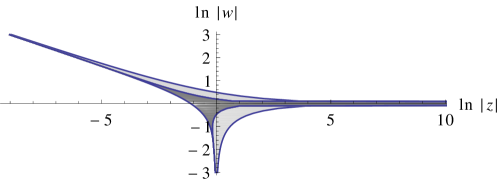
Figure 7: A vortex amoeba with $\hat{P}(z,w)=(1-Jw)(1-w)^{n-1}-1/z$, ($J=-1,\,n=3$). The light and dark regions are the areas where ${\rm Ln}$ is $2$ to $1$ and $4$ to $1$ respectively. The rightmost curve corresponds to $(z,w)=({\rm e}^{x},{\rm e}^{y})$, while the interior curve is $(z,w)=({\rm e}^{x},{\rm e}^{y+i\pi})$ and this latter curve intersects the leftmost curve $(z,w)=({\rm e}^{x},{\rm e}^{y+\phi_{*}(y)})$ at finite values of $x$ and $y$, so that the lower boundary of the amoeba is composed of the finite segment of $\phi=\phi_{*}(y)$ and the unbounded segments of $\phi=\pi$.

The $4$ to $1$ region contains the amoeba origin $(0,0)$ and consequently intersects with the unit torus $T^{2}$. This means that $\hat{P}(z,w)$ vanishes at the $4$ points constituting ${\rm Ln}^{-1}(0,0)$: these form $2$ complex conjugate pairs which we denote by $p,\bar{p}$ and $q,\bar{q}$. The connection $A$ on $\det E^{+}$ is now defined over the $4$-punctured torus $T^{2}_{p,\bar{p},q,\bar{q}}$ and $A$ has the non-trivial holonomy

$$\exp\left[\int_{C}A\right]$$ (101)

e.g., when $C$ encircles one of these $4$ points. The K-theory statement has now enlarged: one has

$$\widetilde{K}O(T^{2}_{p,\bar{p},q,\bar{q}})={\bf Z_{2}}\oplus{\bf Z_{2}}\oplus{\bf Z_{2}}\oplus{\bf Z_{2}}\oplus{\bf Z_{2}}$$ (102)

reflecting the two extra zeroes.

It is interesting, from a physical point of view to analyse this example in more detail. If we consider the vortex full lattice corresponding to the hexagonal tiling of figure 1: i.e. figure 5 with $n=2$, weights from figure 1 but $J_{2z}=-a$. We then obtain the polynomial

$$\hat{P}(z,w)=c^{2}-a^{2}w^{2}-b^{2}/z\,,$$ (103)

where $z$ and $w$ are on the unit torus. The partition function in this case can be analysed in detail using the techniques of Nash_OConnor_jphysa:2009 ; Nash:1995ba ; Nash:1996kn .

For completeness let us continue to use the same weights, and summarise the result in the vortex free case corresponding to $n=2$ in figure 5. For $\hat{P}(z,w)$ we have $\hat{P}=(c-aw)^{2}-b^{2}/z$; which has zeros at $(z,w)=({\rm e}^{i\Theta/2},{\rm e}^{i\Phi})$ and $(\bar{z},\bar{w})$. There are $2NM$ dimers and, in the thermodynamic limit, the logarithm of the bulk partition function per dimer, $W=\frac{\ln Z}{2NM}$, is given by

$$W(a,b,c)=\ln c+\frac{\Theta}{\pi}\ln(b/c)+\frac{1}{2\pi i}({\it li}_{2}(\frac{a}{c}{\rm e}^{i\Theta})-{\it li}_{2}(\frac{a}{c}{\rm e}^{-i\Theta}))$$ (104)

with

$$\sin(\Theta)=\frac{b}{2r}\ ,\quad\sin(\Phi)=\frac{a}{2r}\quad{\rm and}$$ (105)

$$\kern-24.0ptr=\frac{abc}{\sqrt{(a+b+c)(-c+a+b)(c-a+b)(c+a-b)\,}}\,.$$ (106)

One finds

$$\lim_{N,M\rightarrow\infty}\frac{Z(N,M)}{{\rm e}^{2NMW_{Vortex}(a,b,c)}}=Z_{Dirac}(\tau,\theta,\phi)=\frac{1}{2}\sum_{u,v=0}^{1/2}\left|\frac{\theta[{}^{\theta+u}_{\phi+v}](0|\tau)}{\eta(\tau)}\right|\,,$$ (107)

with

$$\tau=\frac{2Nb}{Ma}{\rm e}^{i(\Theta+\Phi)}\,.$$ (108)

and $\theta[{}^{\theta+u}_{\phi+v}](0|\tau_{v})$ and ${\eta(\tau_{v})}$ are the Jacobi $\theta$-function and Dedekind $\eta$-function respectively. This is the partition function for a Dirac Fermion propagating on the continuum torus with modular parameter $\tau$ and a flat connection, but with holonomies ${\rm e}^{2\pi i\theta}$ and ${\rm e}^{2\pi i\phi}$ round the cycles of the torus.

The result for the vortex case can be obtained rather simply from those of the one tile example of Nash_OConnor_jphysa:2009 with polynomial $\hat{P}=c-aw-b/z$. The bulk free energy is given by

$$W_{vortex}(a,b,c)=\frac{1}{2}W(a^{2},b^{2},c^{2})\,.$$ (109)

There are now four zeros which come in complex conjugate pairs. These occur at $(z,w)=({\rm e}^{i\Theta_{v}},{\rm e}^{i\Phi_{v}})$ and $(z,w)=({\rm e}^{i(\Theta_{v})},{\rm e}^{i(\Phi_{v}+\pi)})$, together with their complex conjugates, where $\Theta_{v}$ and $\Phi_{v}$ are obtained from $\Theta$ and $\Phi$ by sending $a$,$b$ and $c$ to $a^{2}$, $b^{2}$ and $c^{2}$ respectively.

Expanding around the zeros of the polynomial one can easily establish that for large $M$ and $N$ we have

$$\lim_{N,M\rightarrow\infty}\frac{Z_{Vortex}(N,M)}{{\rm e}^{2NMW_{Vortex}(a,b,c)}}=\frac{1}{2}\sum_{u,v=0}^{1/2}\left|\frac{\theta[{}^{\theta+u}_{\phi+v}](0|\tau_{v})}{\eta(\tau_{v})}\right|^{2}\,.$$ (110)

where

$$\tau_{v}=\frac{Nb^{2}}{Ma^{2}}{\rm e}^{i(\Theta_{v}+\Phi_{v})}\ .$$ (111)

In general the holonomies $\theta$ and $\phi$ depend on the details of how the system is scaled to the continuum limit. For $a=b=c=1$ in Nash_OConnor_jphysa:2009 we found that these holonomies depend on the conjugacy class of $L$ and $M$ ${\rm mod}$ $6$ with $(\theta,\phi)=(\frac{1}{2}-\frac{q}{6},\frac{1}{2}+\frac{p}{6})$ for $(L,M)=(q\;{\rm mod}\;6,p\;{\rm mod}\;6)$. When $(\theta,\phi)=(0,0)$ then the term $u=v=0$ in (110) is zero, the expression is modular invariant and the system has central charge $c=2$; as can be read off from the decrease of the finite size effects in the cylinder limit.

In summary: The leading finite size correction to the vortex free partition function is given by the continuum limit of a free Dirac Fermion. In contrast for the vortex full configuration described above, the finite size corrections corresponds to two Dirac Fermions; however, the partition function is not a free sum over spin structures, rather the spin structures are constrained to be equal, so these form a rather natural Fermion doublet.

Example A pinch

Consider the graph of figure 3 with

$$\hat{P}(z,w)=c-b\,z-\frac{a}{w}-\frac{d}{wz}$$ (112)

This gives a Harnack curve ${\cal C}$ and ${\rm Ln}:{\cal C}\longrightarrow{\bf R}^{2}$ is $2$ to $1$ everywhere. However, if some edge weights are negative then the amoeba ${\cal A}({\cal C})={\rm Ln}({\cal C})$ can develop a pinch singularity at some point $p\in{\cal A}$: at this point ${\rm Ln}^{-1}(p)$ is no longer even discrete, but continuous, as we shall now discover.

Representing the curve ${\cal D}$ by solving $\hat{P}(z,w)$ in (112) for $w(z)$ the Jacobian condition

$$\det({\rm J(Ln)})=0\,,$$ (113)

with $z={\rm e}^{x+i\theta}$, $w={\rm e}^{y+i\phi}$ can be reduced to

$$u(-\theta)\partial_{\theta}u(\theta)+u(\theta)\partial_{\theta}u(-\theta)=0,\qquad u(\theta)=\frac{a+d\,{\rm e}^{-x-i\theta}}{c-b\,{\rm e}^{x+i\theta}}$$ (114)

This has the solutions $\theta=0,\pi$ which are the boundary of the amoeba; but it also has the solution $x_{p}$ where

$$x_{p}=-\frac{1}{2}\ln\left(-\frac{ab}{cd}\right)\quad\hbox{ with }\quad y_{p}=\frac{1}{2}\ln(\frac{a^{2}}{c^{2}})\,.$$ (115)

This gives the pinch point $p$ which we write as $p=(x_{p},y_{p})$ and ${\rm Ln}^{-1}(p)$ is a circle. If all edge weights are unity except $a$ then we find that

$$p=\left(-\frac{1}{2}\ln(-a),\ln(-a)\right)$$ (116)

and we note the necessity for negative $a$. We show a plot with the pinch in figure 8.

One can easily check that negative $a$ corresponds to a vortex full configuration on the lattice tiled with the fundamental tile of figure 3.

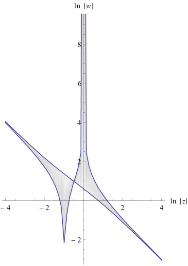
Figure 8: A non-Harnack amoeba with a pinch for $\hat{P}(z,w)=1-z-\frac{\textstyle a}{\textstyle w}-\frac{\textstyle 1}{\textstyle wz}$ and $a=-\sqrt{7}$

Example A shrunken area

Next we come to an example where it is simple to demonstrate the area shrinking imposed on a non-Harnack curve. We take the second graph on figure 1 for which

$$\hat{P}(z,w)=a_{1}c_{2}+a_{2}c_{1}+b_{1}d_{2}+b_{2}d_{1}-\frac{a_{1}a_{2}}{z}-c_{1}c_{2}\,z-d_{1}d_{2}\,w-\frac{b_{1}b_{2}}{w}\,.$$ (117)

We have already considered this polynomial before and its amoeba is displayed in figure 2 for the case where

$$\hat{P}(z,w)=2D-z-\frac{1}{z}-w-\frac{1}{w},\quad D=2+2\cosh(t)$$ (118)

This is a standard amoeba with ${\rm Area\,}({\cal A(C)})=\pi^{2}{\rm Area\,}(\Delta)\,$.

It turns out that the curve ${\cal C}$ is non-Harnack if $D<2$—an impossibility in the present equation for $\hat{P}(z,w)$. However, if $a_{1}=a_{2}^{-1}=-{\rm e}^{t_{1}}$, $b_{1}=b_{2}^{-1}={\rm e}^{t_{2}}$ and all other weights are set to unity—so that we have a vortex full lattice—then

$$\hat{P}(z,w)=2D-z-\frac{1}{z}-w-\frac{1}{w},\quad D=\cosh(t_{2})-\cosh(t_{1})$$ (119)

and $D<2$ becomes accessible.

This means that ${\rm Ln}$ becomes singular but it also means that the second amoeba shrinks: denoting the two amoeba by ${\cal A(C}_{1})$ and ${\cal A(C}_{2})$ respectively, one must have

$${\rm Area\,}({\cal A(C}_{2}))<{\rm Area\,}({\cal A(C}_{1}))=2\pi^{2}\,.$$ (120)

In figure 9 we show the ${\cal A(C)}$ for $D>2$ and $D<2$ and the shrink is clearly manifest. Note that for $D\geq 2$ the curve always has a compact oval and ${\cal A(C)}=2\pi^{2}$ while for $0<D<2$, we have ${\cal A(C)}<2\pi^{2}$. The case $D=0$ is rather special in that the amoeba consists of the two lines $y=\pm x$ and ${\cal A(C)}=0$.

We see that the topological type of ${\cal C}$ has degenerated when $D<2$: it has lost a compact oval. For $D=2$ the curve ${\cal C}$ is still Harnack though there is a real node at the origin $p=(0,0)$ of ${\cal A(C)}$; but for $D<2$ there is a more serious singularity and ${\rm Ln}^{-1}(p)$ is no longer discrete.

If we focus on the physical weights we see that introducing vortices, as above, changes $D=\cosh(t_{1})+\cosh(t_{2})$ to $D=\cosh(t_{1})-\cosh(t_{2})$ so that for $t_{2}=0$, with $\cosh(t_{1})<3$, we are in the non-Harnack case. Further—even in the presence of vortices—if $\cosh(t_{2})=3$ we have $D=2$: the degenerate Harnack case with no compact oval; but, as $t_{2}$ is increased still further, the curve is Harnack with a compact oval.

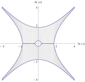
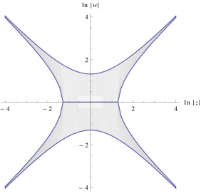
Figure 9: The shrinking phenomenon displayed: both amoeba have $\hat{P}(z,w)=2D-z-z^{-1}-w-w^{-1}$ but the larger one has $D>2$ ($D=2.05$) and is Harnack, while the smaller one has $D<2$ ($D=1$) and is non-Harnack.

We shall now investigate the singularity at the origin: choosing $z={\rm e}^{x+i\theta},\;w={\rm e}^{y+i\phi}$ we obtain

$$\hat{P}(z,w)=2D-2\cosh(x+i\theta)-2\cosh(y+i\phi)$$ (121)

so that ${\cal C}$ is given by the equation

$$D-\cosh(x+i\theta)-\cosh(y+i\phi) =0$$ (122)

$$\Rightarrow y+i\phi =\mathop{\rm arccosh}\nolimits(D-\cosh(x+i\theta))$$

Thus $Ln$ is given by

$${\rm Ln}:{\cal C}\longrightarrow{\bf R}^{2}$$ (123)

$$\qquad(z,w)\longmapsto(x,\Re(\mathop{\rm arccosh}\nolimits(D-\cosh(x+i\theta)))$$

and for the Jacobian we have

$$J({\rm Ln})=\left(\begin{matrix}1&0\\ \partial_{x}\Re(\mathop{\rm arccosh}\nolimits(D-\cosh(x+i\theta)))&\partial_{\theta}\Re(\mathop{\rm arccosh}\nolimits(D-\cosh(x+i\theta)))\\ \end{matrix}\right)$$ (124)

so singularities occur when

$$\partial_{\theta}\Re(\mathop{\rm arccosh}\nolimits(D-\cosh(x+i\theta))) =0$$ (125)

$$\Rightarrow\Re\left\{\frac{-i\sinh(x+i\theta)}{\sqrt{(D-\cosh(x+i\theta))^{2}-1}}\right\} =0$$

Now suppose $x=0$, then we have the condition

$$\Re\left\{\frac{\sin(\theta)}{\sqrt{(D-\cos(\theta))^{2}-1}}\right\}=0$$ (126)

and we see the usual real node solutions for $\theta=0,\pi$ but, also solutions for those $\theta$ which satisfy

$$D-\cos(\theta)-1<0$$ (127)

which requires $D<2$.

Now note that a point on the amoeba with $x=0$ has coordinates

$$(0,\Re(\mathop{\rm arccosh}\nolimits(D-\cos(\theta))))=(0,0),\quad\text{when }D-\cos(\theta)<1$$ (128)

since $\mathop{\rm arccosh}\nolimits(z)$ is pure imaginary when $z<1$. Hence ${\rm Ln}$ maps all these singular points to the amoeba origin $p$ and ${\rm Ln}^{-1}(p)$ is no longer discrete when $D<2$ but consists of the interval $[-\cos^{-1}(D-1),\cos^{-1}(D-1)]$.

IX Conclusions

We have found that the geometrical constructs of connection and curvature can be very effective tools to analyse the structure of dimer models, particularly on the torus with and without punctures. One is led naturally to topological invariants including holonomy, Chern classes as well as K-theory. Another effective tool, to which we have frequent recourse, is the spectral curve ${\cal C}$: an object which has dual life as a Harnack curve and the characteristic polynomial of a bipartite dimer model. The amoeba ${\cal A(C)}$ of ${\cal C}$ also plays a central role: for example it determines the phase diagram of the model and in the presence of vortices it can even have singularities and facilitate the uncovering of the rich Fermionic structure underlying dimer models.

Before finishing we wish to make an observation about Pfaffians and holonomy: in this work the Kasteleyn matrix, $K$, is a model for a discrete Dirac operator and $\mbox{Pfaff}\,(K)$ is of central importance. Further when the vector bundle of positive eigenvalues of $iK$ has $\;\mbox{tr}\;(F)=0$ the quantity $\;\mbox{tr}\;(A)$—or just $A$ in the $U(1)$ case—is the simplest example of a Chern-Simons form and its exponentiated integral over $C$ is the holonomy invariant

$$\exp\left[\int_{C}A\right]$$ (129)

This expression is naturally a geometric invariant with values in ${\bf R/Z}$ just as in the higher dimensional Chern-Simons cases.

The same two quantities turn up in studies of global anomalies in the path integral for type II superstring theories with D-branes FreedWitten . There the world sheet measure contains the crucial product

$$\mbox{Pfaff}\,(D)\exp\left[\int_{\partial\Sigma}A\right]$$ (130)

with $\mbox{Pfaff}\,(D)$ the Pfaffian of the world sheet Dirac operator and $\partial\Sigma$ the boundary of the world sheet $\Sigma$. There are also some intricate discussions of holonomy and Pfaffians in Wittencondensedmatter . This parallel may repay further study.

We have only just begun the study of dimer models with vortices. As is evident from our study there is a rich structure to be studied further here.

One could extend the study to models where lattice weights are elements of a finite Abelian group, instead of just being real, or complex, numbers. Furthermore when dimer model partition functions are realised as the Pfaffian of a Dirac operator one could further add a gauge field in the form of holonomy elements linking the different lattice sites. This latter step would take us into the realm of lattice gauge theory proper.

In summary, our current study has revealed that the presence of vortices can alter the phase diagram of a dimer model, and change the finite size corrections from a system with central charge, $c=1$ to one with central charge $c=2$, corresponding to a Dirac doublet rather than the standard vortex free case of a Dirac singlet.

Further properties and physical consequences of the presence of vortices are discussed separately in inprep .

Appendix A K-theory

We present here some brief selected facts on K-theory that are more in place in this appendix than in the main body of the paper.

K-theory is a generalised cohomology theory of real, complex or quaternionic vector bundles over a base space $M$. We shall not consider quaternionic vector bundles. K-theory places to the fore simplifications that occur when the rank of the bundle is large enough compared to $\dim M$: the dimension of $M$.

K-theory defines two rings $K(M)$ and $\widetilde{K}(M)$ arising from $\hbox{\it Vect}\,(M)$ the set of all (isomorphism classes) of vector bundles over $M$ and these are related by

$$K(M)=\widetilde{K}(M)\oplus{\bf Z}$$ (131)

We shall be concerned with $\widetilde{K}(M)$ which is called the reduced K-theory of $M$. The elements of $\widetilde{K}(M)$ are equivalence classes of vector bundles where, denoting an equivalence class for a bundle $E$ by $[E]$, two bundles $E$ and $F$ are equivalent (also called stably equivalent) if the addition of a trivial bundle to each of them renders them isomorphic: i.e.

$$E\oplus I^{j}\simeq F\oplus I^{k}$$ (132)

we can then record this by writing $[E]\mathop{\sim}\limits^{s}[F]$.

In K-theory the ring operations of sum and product are induced by direct sum and tensor product of bundles respectively—as required, multiplication is also distributive over addition.

So far our bundles can be real or complex but now we shall distinguish between these two types. We deal with the complex case first. Let $\hbox{\it Vect}_{k}(M,{\bf C})$ be the set of rank $k$ complex vector bundles over $M$ and let $n=\dim M$ denote the real dimension of $M$. Then a key result is: if $E_{k}\in\hbox{\it Vect}_{k}(M,{\bf C})$ and $p=[n/2]$—the smallest integer not greater than $n/2$—then

$$E_{k}\simeq F_{p}\oplus I^{k-p}$$ (133)

for some rank $p$ bundle $F_{p}$. One can check that this means that

$$\hbox{\it Vect}_{k}(M,{\bf C})\simeq\widetilde{K}(M),\quad\hbox{ for }k>n/2$$ (134)

So that making the rank $k$ of a bundle $E$ larger than $n/2$ does not change the K-theory element $[E]\in\widetilde{K}(M)$; a bundle with $k>n/2$ is said to be in the stable range.

Now we turn to real vector bundles—i.e. the set $\hbox{\it Vect}_{k}(M,{\bf R})$. Here the key result is similar in character but the stable range is different. One also needs some notation to distinguish K-theory for real vector bundles from that for complex vector bundles; we do this by writing mod $\widetilde{K}O(M)$ for the real case and $\widetilde{K}(M)$ for the complex case. Now the key result is: if $E_{k}\in\hbox{\it Vect}_{k}(M,{\bf R})$—then

$$E_{k}\simeq F_{n}\oplus I^{k-n},\quad\hbox{ when }k>n$$ (135)

for some rank $n$ bundle $F_{n}$. This in turn yields the result that

$$\hbox{\it Vect}_{k}(M,{\bf R})\simeq\widetilde{K}O(M),\quad\hbox{ for }k>n$$ (136)

and the stable range for real vector bundles is therefore $k>n$.

Characteristic classes play an important role in K-theory and, for complex vector bundles, a prominent role is played by the Chern character: if, for simplicity, we specialise to the case the bundle $E$ has a connection $A$ with curvature $F_{A}$, then the Chern character $ch\,(E)$ is defined by

$$ch\,(E)=\;\mbox{tr}\;\exp\left[\frac{iF_{A}}{2\pi}\right]$$ (137)

and it satisfies

$$ch\,(E\oplus F) =ch\,(E)+ch\,(F)$$ (138)

$$ch\,(E\otimes F) =ch\,(E)\,ch\,(F)$$

This in turn means that the map

$$ch: \widetilde{K}(M)\longrightarrow\bigoplus_{i>0}H^{2i}(M;{\bf Q})$$ (139)

$$[E]-[F]\longmapsto ch\,(E)-ch\,(F)$$

is a ring homomorphism; while, for real vector bundles there is the ring homomorphism

$$ch: \widetilde{K}O(M)\longrightarrow\bigoplus_{i>0}H^{4i}(M;{\bf Q})$$ (140)

$$[E]-[F]\longmapsto ch\,(E)-ch\,(F)$$

However none of these maps detects torsion in the K-theory. Note that a complex vector bundle of rank $k$ has an underlying real vector bundle $E_{R}$ of real rank $2k$.

For the spheres $S^{n}$ one has the Bott periodicity results

K~(Sn)Z0K~​O​(Sn+8)=K~​O​(Sn) K~O(Sn)Z𝐙2𝐙20Z000missing-subexpression~𝐾superscript𝑆𝑛2~𝐾superscript𝑆𝑛missing-subexpressionfragments fragments~𝐾(S𝑛)Z0missing-subexpression~𝐾𝑂superscript𝑆𝑛8~𝐾𝑂superscript𝑆𝑛missing-subexpressionfragments fragments~𝐾O(S𝑛)ZfragmentsZ2fragmentsZ20Z000\begin{aligned} &\widetilde{K}(S^{n+2})=\widetilde{K}(S^{n})\\ &\begin{tabular}[]{|*{3}{c|}}\hline\cr$n{\rm\,mod\,}2$&0&1\\ \hline\cr\vrule height=12.0pt,width=0.0pt$\widetilde{K}(S^{n})$&{\bf Z}&0\\ \hline\cr\end{tabular}\\ \end{aligned}\qquad\begin{aligned} &\widetilde{K}O(S^{n+8})=\widetilde{K}O(S^{n})\\ &\begin{tabular}[]{|*{9}{c|}}\hline\cr$n{\rm\,mod\,}8$&0&1&2&3&4&5&6&7\\ \hline\cr\vrule height=12.0pt,width=0.0pt$\widetilde{K}O(S^{n})$&{\bf Z}&${\bf Z}_{2}$&${\bf Z}_{2}$&0&{\bf Z}&0&0&0\\ \hline\cr\end{tabular}\\ \end{aligned}

nmod 201nmod 801234567nmod 201nmod 801234567 (141)

and we notice $\widetilde{K}O(S^{n})$ contains torsion even though $H^{*}(S^{n};{\bf Z})$ is torsion free.

While, for general $M$, if $S\wedge M$, or $SM$ for short, denotes the reduced suspension of $M$ (which has the property that $SS^{n}\simeq S^{n+1}$); and one defines $\widetilde{K}^{-1}(M)$ by $\widetilde{K}^{-1}(M)=\widetilde{K}(SM)$ (and similarly for $\widetilde{K}O(M)$), then one has $\widetilde{K}^{n+2}(M)=\widetilde{K}^{n}(M)$ and $\widetilde{K}O^{n+8}(M)=\widetilde{K}O^{n}(M)$.

When two spaces $X$ and $Y$ are joined at a point they are denoted by $X\vee Y$ and one has $\widetilde{K}O(X\vee Y)=\widetilde{K}O(X)\oplus\widetilde{K}O(Y)$ and similarly for $\widetilde{K}(X\vee Y)$. Thus for a bouquet of circles one needs only $\widetilde{K}O(S^{1})$ or $\widetilde{K}(S^{1})$ as the case may be.

For Cartesian products $X\times Y$ one takes the space $X\wedge Y$—defined by $X\wedge Y=(X\wedge Y/X\vee Y)$—and uses the fact that

$$\widetilde{K}^{-n}(X\times Y)=\widetilde{K}^{-n}(X\wedge Y)\oplus\widetilde{K}^{-n}(X\vee Y)$$ (142)

and similarly for $\widetilde{K}O$. It is now straightforward to calculate the various K-theory rings that we require and, to this end, we would like to compare the real and complex K-theories of $S^{2}$ and $T^{2}$ for which we find that

$$\widetilde{K}(S^{2}) ={\bf Z}\qquad\widetilde{K}O(S^{2})={\bf Z_{2}}$$ (143)

$$\widetilde{K}((T^{2}) ={\bf Z}\qquad\widetilde{K}O(T^{2})={\bf Z_{2}}\oplus{\bf Z_{2}}\oplus{\bf Z_{2}}$$

and we see that the complex K-theories of $S^{2}$ and $T^{2}$ coincide but that the real K-theories differ considerably.

For $S^{2}$ one also knows the appropriate generators: if $H$ is isomorphic to the Hopf, or monopole line bundle, over $S^{2}$ which has $c_{1}(H)=1$ then $\widetilde{K}(S^{2})$ has generator $[H]-[I]$, whereas, if $H_{R}$ is the underlying real vector bundle of rank $2$ to $H$ then $\widetilde{K}O(S^{2})$ has generator $[H_{R}]-[I^{2}]$. One can check explicitly that $H_{R}\oplus H_{R}\simeq I^{4}$ so that $[H_{R}]-[I^{2}]$ is of order $2$.

For $T^{2}$, if $f:T^{2}\longrightarrow S^{2}$ is a map of degree $1$, then $f^{*}H$ is a line bundle over $T^{2}$ with $c_{1}(f^{*}H)=1$ and $[f^{*}H)]-[I]$ generates $\widetilde{K}(T^{2})$; also the underlying real bundle $f^{*}H_{R}$ will provide one of the generators of $\widetilde{K}O(T^{2})$.

We have torsion in our holonomy calculations so we make recourse to $\widetilde{K}O$ and observe that, for the punctured tori, which are bouquets of circles, the above implies that

$$\widetilde{K}(T^{2}_{p,\bar{p}})=0$$ (144)

$$\widetilde{K}(T^{2}_{p,\bar{p},q,\bar{q}})=0$$

while for $\widetilde{K}O$ one has

$$\widetilde{K}O(T^{2}_{p,\bar{p}}) ={\bf Z_{2}}\oplus{\bf Z_{2}}\oplus{\bf Z_{2}}$$ (145)

$$\widetilde{K}O(T^{2}_{p,\bar{p},q,\bar{q}}) ={\bf Z_{2}}\oplus{\bf Z_{2}}\oplus{\bf Z_{2}}\oplus{\bf Z_{2}}\oplus{\bf Z_{2}}\,.$$

The bundle $E^{+}_{R}$ has an Euler class $e(E^{+}_{R})$, and Stieflel-Whitney classes $w_{1}(E^{+}_{R})$ and $w_{2}(E^{+}_{R})$: these classes possess the properties $e(E^{+}_{R})=c_{1}(E^{+})$, $w_{2}(E^{+}_{R})=c_{1}(E^{+}){\rm\,mod\,}2$ and $w_{1}(E^{+}_{R})=0$ since $E^{+}_{R}$ is oriented.

In the case of non-bipartite graphs—cf. figure 4 above—we found that the complex line bundle $E^{+}$ over $T^{2}$ had $c_{1}(E^{+})=-1$, which is fine for $\widetilde{K}(T^{2})$. Thus $e(E^{+}_{R})=1$, $w_{2}(E^{+}_{R})=1$ and $w_{1}(E_{R}^{+})=0$. However to detect the ${\bf Z_{2}}$ holonomy around the two homology cycles, which turns up when the curvature vanishes, we should pass from $E^{+}$ to $E^{+}_{R}$ and use $\widetilde{K}O(T^{2})$.

For bipartite graphs $E^{+}$ one has $c_{1}(E^{+})=0$, while $e(E^{+}_{R})=0$ and $w_{2}(E^{+}_{R})=w_{1}(E^{+}_{R})=0$.

References

- (1) Kenyon R., Okounkov A. and Sheffield S., “Dimers and Amoebae”, Ann. Math 163, 1019–1056, 2006, [arXiv:math-ph/0311005].
- (2) Kenyon R. and Okounkov A., “Planar dimers and Harnack curves”, Duke Math. J., 131, 499–524, 2006. [arXiv:math/0311062].
- (3) Cimasoni D. and Reshetikhin N., “Dimers on surface graphs and spin structures. I” Comm. Math. Phys., 275, 187–208, 2007. [ arXiv:math-ph/0608070]
- (4) Cimasoni D.and Reshetikhin N., “Dimers on surface graphs and spin structures. II” Comm. Math. Phys., 281, 445–468, 2008. [arXiv:math-ph/0704.0273]
- (5) Broomhead N., “Dimer models and Calabi-Yau algebras”, Memoirs of the Amer. Math. Soc, 215, 2012, DOI: http://dx.doi.org/10.1090/S0065-9266-2011-00617-9, [arXiv:math.AG/0901.4662]
- (6) Kasteleyn P. W., “Dimer statistics and phase transitions”, J. Math. Phys., 4, 287–298, 1963.
- (7) Fisher M. E., “On the dimer solution of planar Ising models”, J. Math. Phys., 4, 1776–1781, 1966.
- (8) Nagle J. F., Yokoi C. S. O. and Bhattacharjee S. M., “Dimer models on anisotropic lattices”, Phase transitions and critical phenomena vol. 13, edited by: Domb C. and Lebowitz J. L., Academic Press, (1989).
- (9) Hanany A. and Kennaway K. D., “Dimer models and toric diagrams”, [arXiv:hep-th/0503149]
- (10) Okounkov A., Reshetikhin N. and Vafa C., “Quantum Calabi-Yau and classical crystals”, Progress in Mathematics 244, The Unity of Mathematics (In Honor of the Ninetieth Birthday of I. M. Gelfand) edited by: Etingof P., Retakh V., Singer I. M., Birkhaüser, (2006). [arXiv:hep-th/0309208]
- (11) Franco S., Hanany A., Kennaway K. D., Vegh D. and Wecht B., “Brane Dimers and Quiver Gauge Theories”, J. High Energy Phys., 0601:096, 2006. [arXiv:hep-th/050411]
- (12) Feng B., He Y., Kennaway K. D. and Vafa C., “Dimer Models from Mirror Symmetry and Quivering Amoebae”, Adv. in Theor. and Math. Phys., 12, 489–545, 2008. [arXiv:hep-th/0511287]
- (13) Dijkgraaf R, Orlando D. and Reffert S. “Dimer Models, Free Fermions and Super Quantum Mechanics”, Adv. in Theor. and Math. Phys., 13, 1255–1315, 2009. [arXiv:hep-th/0705.1645v2]
- (14) Nash C., and O’Connor D., “Topological Phase Transitions and Holonomies in the Dimer Model”, J. Phys. A, 42 (2009) 012002, [arXiv:hep-th/0809.2960].
- (15) Mikhalkin G. and Rullgård H., “Amoebas of Maximal area”, Internat. Math. Res. Notices, 9 441–451, 2001. [arXiv:math/0010087].
- (16) Nash C. and O’Connor D., “The Zero Temperature Phase Diagram of the Kitaev Model”, Phys. Rev. Lett., 102 (2009), 147203; [arXiv:hep-th/0812.0099[cond-mat].
- (17) Mikhalkin G., “Amoebas of algebraic varieties and tropical geometry”, Different faces of geometry, edited by: Donaldson S., Kluwer, (2004). [arXiv:math/0403015]
- (18) Nash C. and O’Connor D. “Modular invariance of finite size corrections and a vortex critical phase,” Phys. Rev. Lett., 76 (1996), 1196 doi:10.1103/PhysRevLett.76.1196 [arXiv:hep-th/9506062].
- (19) Nash C. and O’Connor D., “Modular invariance, lattice field theories and finite size corrections,” Annals Phys., 273 (1999) 72 doi:10.1006/aphy.1998.5868 [arXiv:hep-th/9606137].
- (20) Freed D. and Witten E., “Anomalies in String Theory with D-Branes”, Asian J. Math., 3:819, (1999) [arXiv:hep-th/9907189]
- (21) Witten E., “Fermion Path Integrals And Topological Phases”, Rev. Mod. Phys. 88, (2016), 035001, [arXiv:hep-th/1508.04715]
- (22) Nash C., and O’Connor D., in preparation.