Abstract: In this study, we investigate a new type of a surface curve called a new $D$-type special curve. Also, we show that this special curve is more generally than a geodesic curve or an asymptotic curve. Then, we give the necessary and sufficient conditions for a curve to be the new $D$-type special curve using Frenet frame in Galilean space. We investigate some corollaries by taking account of a new $D$-type special curve as a helix, a salkowski and an anti-salkowski. After all, for the sake of visualizing of this study, we plot some examples for this surface pencil (i.e. surface family).

Key words: New $D$-type special curve, Geodesic curve, Isoparametric curve Parametric surface, Galilean space.

1 Introduction

One of the important problems arising when studying geometry is to determine its properties by using physical,computational and experimental methods. For this aim, many researchers have been focused on the curve and surface theory because of having many applications to that of various branch of science and engineering. As far as we know, the Frenet-Frame based system is commonly used in physics as well confined particle motion around the design orbit. The coordinate system around the design orbit is called  the Serret-Frenet frame and this  frame can be achieved using some special functions related to Hamiltonian, [8, 10].

On the other hand Galilean geometry is one of the real Cayley-Klein  Geometries to that of motions are the Galilean transformations of classical kinematics, [17]. The decades have witnessed a rapid increase in study of Galilean and Pseudo-Galilean space in [3, 4, 12, 9].

Besides all studies mentioned above parametric of a surface pencil with a common spatial geodesic, asymptotic and geometric applications for computer science is have a great importance for those who study multidisciplinary science and searching relations between theoretical and applied methodology, in [5, 2, 11, 16].

Roughly speaking, this work serves the purpose of defining a new type surface curve which called a new D-type curve using Frenet-frame in Galilean space. Furthermore, a $D-$type curve  firstly defined as $\left\langle\eta_{1},E_{0}\right\rangle=\lambda=const.$ in [7], then we introduce a new D-type curve given by $\left\langle\eta_{1},E_{0}\mathbf{\wedge}t\right\rangle=\lambda=const.$ based on the first definition. We show that this new $D-$type curve is more general than a geodesic or asymptotic curve.

This study is organized as follows: In preliminary part, we give Galilean space $G_{3}$ and give some basic definitions and concepts of it. Then, we define a new $D$-type special curve of this space. Following section is devoted to surfaces with a common new type special curve in $G_{3}$ . We give some characterizations for this new type curve. Notice that new $D$-type special curves are also satisfies being helix,salkowski and anti-salkowski curves. At the end of the study, we give some examples for this surface pencil.

2 Preliminaries

The Galilean space $\mathbf{G}_{3}$ is a one of the real Cayley-Klein space, which has the projective metric of signature $(0,0,+,+)$.The absolute figure of the Galilean space consists of an ordered triple$\{\omega,f,I\}$ in which $\omega$ is the ideal (absolute) plane, $\ f$  is the line (absolute line) in $\omega$ and $I$ is the fixed elliptic involution of points of $f$. For more properties of Galilean space can be found in [1, 14].

A plane is said to be Euclidean if it contains $f$, otherwise it is said to be isotropic. In the given affine coordinates, isotropic vectors are of the form $(0,x_{2},x_{3})$, whereas Euclidean planes are of the form $x=const.$ The induced geometry of a Euclidean plane is Euclidean and of an isotropic plane isotropic (i.e. 2-dimensional Galilean or flag-geometry).

Definition 2.1

Let $a$$=$ $\left(a_{1},a_{2},a_{3}\right)$ and $b$$=$ $\left(b_{1},b_{2},b_{3}\right)$ be vectors in $\mathbf{G}_{3}.$ A vector $a$ is said to be isotropic if $a_{1}=0$, otherwise it is said to be non-isotropic. Then the Galilean scalar product of these vectors is given by

$$\left\langle a,b\right\rangle=\left\{\begin{array}[]{cc}a_{1}b_{1},&\text{if }a_{1}\neq 0\text{ or }b_{1}\neq 0\\ a_{2}b_{2}+a_{3}b_{3},&\text{if \ }a_{1}=0\text{ and }b_{1}=0\end{array}\right.,$$

[15] .

Definition 2.2

Let $a$$=$ $\left(a_{1},a_{2},a_{3}\right)$ and $b$$=$ $\left(b_{1},b_{2},b_{3}\right)$ be vectors in $\mathbf{G}_{3},$ the cross product of the vectors $a$ and $b$ is defined by

$$\ a\wedge b=\left|\begin{array}[]{ccc}0&e_{2}&e_{3}\\ a_{1}&a_{2}&a_{3}\\ b_{1}&b_{2}&b_{3}\end{array}\right|=(0,a_{3}b_{1}-a_{1}b_{3},a_{1}b_{2}-a_{2}b_{1}),$$

[15].

Definition 2.3

If an admissible curve $r$ of the class $\mathbf{C}^{r}$ $(r>3)$ in $\mathbf{G}_{3},$ and parametrized by the invariant parameter $s$ , is given by

$$r\left(s\right)=\left(s,f\left(s\right),g\left(s\right)\right).$$

then $s$ is a Galilean invariant of the arc length on $r$.

The moving trihedron is written by

$$t\left(s\right) = r^{\prime}\left(s\right)=\left(1,f^{\prime}\left(s\right),g^{\prime}\left(s\right)\right),$$

$$n\left(s\right) = \frac{r^{\prime\prime}\left(s\right)}{\kappa\left(s\right)}=\frac{1}{\kappa\left(s\right)}\left(0,f^{\prime\prime}\left(s\right),g^{\prime\prime}\left(s\right)\right),$$

$$b\left(s\right) = \frac{1}{\kappa\left(s\right)}\left(0,-g^{\prime\prime}\left(s\right),f^{\prime\prime}\left(s\right)\right),$$

where $t,n$ and $b$ are called the vectors of the tangent, principal normal and binormal of $r\left(s\right),$ respectively, and the curvature $\kappa\left(s\right)$ and the torsion $\tau\left(s\right)$ of the curve $r$ can be given by, respectively,

$$\kappa\left(s\right) = \sqrt{f^{\prime\prime}\left(s\right)^{2}+g^{\prime\prime}\left(s\right)^{2}},$$

$$\tau\left(s\right) = \frac{\det\left(r^{\prime}\left(s\right),r^{\prime\prime}\left(s\right),r^{\prime\prime\prime}\left(s\right)\right)}{\kappa^{2}\left(s\right)}.$$

Frenet formulas can be given as

$$t^{\prime} = \kappa n,$$ (1)

$$n^{\prime} = \tau b,$$

$$b^{\prime} = -\tau n,$$

[13].

Definition 2.4

Let $\left\{t,n,b\right\}$ be the Frenet frame of the differentiable curve in $\mathbf{G}_{3}$. The equations (1) form a rotation motion with Darboux vector $w=\tau t+\kappa b.$ Also momentum rotation vector holds the following conditions

$$t^{\prime}=w\mathbf{\wedge}t\mathbf{,}\text{ }n^{\prime}=w\mathbf{\wedge}n\mathbf{,}\text{ }b^{\prime}=w\mathbf{\wedge}b\mathbf{,}$$

[14]

Besides, the unit vector $E_{0}$ from Darboux vector is obtained by

$$E_{0}=\frac{\tau t+\kappa b}{\left|\tau\right|},$$ (2)

[6].

In the rest of paper, we shall suppose $\kappa\neq{0}$ and $\tau\neq{0}$ at everywhere.

Definition 2.5

Let $\varphi$ is a surface in $\mathbf{G}_{3},$ the equation of a surface in $\mathbf{G}_{3}$ can be expressed as the parametrization

$$\varphi\left(s,\upsilon\right)=\left(\varphi_{1}\left(s,\upsilon\right),\varphi_{2}\left(s,\upsilon\right),\varphi_{3}\left(s,\upsilon\right)\right),\text{ }s,\upsilon\in R,$$

where $\varphi_{1}\left(s,\upsilon\right),\varphi_{2}\left(s,\upsilon\right)$ and $\varphi_{3}\left(s,\upsilon\right)\in\mathbf{C}^{3},$ in [14].

Also, the isotropic normal vector is defined by

$$\eta\left(s,v\right)=\varphi_{s}\mathbf{\wedge}\varphi_{v},$$

where $\varphi_{s}=\frac{\partial\varphi\left(s,v\right)}{\partial s}$ and $\varphi_{v}=\frac{\partial\varphi\left(s,v\right)}{\partial v}$.

Definition 2.6

Let $\varphi$ be a regular surface in $\mathbf{G}_{3}$ with the isotropic surface normal $\eta\left(s,v\right)$ and $r(s)$ be an arc-length parametrized curve on ’$\varphi.$ If the following condition

$$\left\langle\eta_{1},E_{0}\mathbf{\wedge}t\right\rangle=\lambda=const.,$$

is satisfied, then the curve $r(s)$ is said to be a new $D$-type special curve on $\varphi,$ where $E_{0},$ $t$ and $\eta_{1}$ is the unit darboux vector, tangent vector and unit surface normal along the curve $r$, respectively.

Considering Definition 2.6, if $\lambda=0$, then the surface normal $\eta_{1}$ is orthogonal to the principal normal $n,$ i.e, the curve $r(s)$ is an asymptotic curve on $\varphi.$ Similarly, if $\lambda=1$ then the surface normal $\eta_{1}$ and the principal normal $\eta_{1}$ are linearly dependent, it means that the curve $r(s)$ is a geodesic curve on $\varphi.$ Our studies show that the new $D$-type special curves contain both geodesic and asymptotic curves, that is, the new $D$-type special curves are more general then both curves.

3 Surfaces with Common New Type Special Curve in Galilean Space $G_{3}$

Let $\varphi=\varphi\left(s,v\right)$ be a parametric surface on the arc-length parametrized curve $r(s)$ in $\mathbf{G}_{3}.$ The surface is defined by

$$\varphi\left(s,v\right) = r(s)+[\alpha\left(s,v\right)t\left(s\right)+\beta\left(s,v\right)n\left(s\right)$$

$$+\gamma\left(s,v\right)b\left(s\right)],$$

$$L_{1} \leq s\leq L_{2}\text{ and }T_{1}\leq v\leq T_{2},$$

where $\alpha\left(s,v\right),\beta\left(s,v\right)$ and $\gamma\left(s,v\right)$ are smooth functions. $\alpha\left(s,v\right),\beta\left(s,v\right)$ and $\gamma\left(s,v\right)$ are smooth functions and their values indicate, respectively, the extension-like, flexion-like, and retortion-like effects, by the point unit through the time $v$, starting from $r(s),$ (see [9]).

Our starting point is to provide the necessary and sufficient conditions for the given curve $r(s)$ to be a new $D-$type special curve on the surface $\varphi=\varphi\left(s,v\right).$

The unit surface normal $\eta_{1}$ can be given

$$\eta_{1}=\cos\theta n+\sin\theta b,$$

where $n$ and $b$ are the principal normal and binormal of $r\left(s\right),$ respectively. Now we give the necessary and sufficient conditions for an isoparametric curve $r(s)$ to be a common special new $D-$type curve on $\varphi\left(s,v\right).$

The isotropic normal $\eta\left(s,v\right)$ of the surface is given by

$$\eta\left(s,v\right)=\varphi_{s}\mathbf{\wedge}\varphi_{v},$$ (4)

from (3)

$$\varphi_{s} = \left(1+\alpha_{s}\right)t+\left(k\alpha+\beta_{s}-\tau\gamma\right)n+\left(\tau\beta+\gamma_{s}\right)b,$$

$$\varphi_{v} = \alpha_{v}t+\beta_{v}n+\gamma_{v}b.$$

Taking account (4), $\eta\left(s,v\right)$ can be given as

$$\eta\left(s,v\right) = \left[-\left(1+\alpha_{s}\right)\gamma_{v}+\left(\tau\beta+\gamma_{s}\right)\alpha_{v}\right]n$$

$$+\left[\left(1+\alpha_{s}\right)\beta_{v}-\left(k\alpha+\beta_{s}-\tau\gamma\right)\alpha_{v}\right]b.$$

.

Let $r(s)$ be a curve on a surface $\varphi\left(s,v\right)$ in $\mathbf{G}_{3}.$ If $r(s)$ is isoparametric curve on this surface, then there exists a parameter $v=v_{0}$ such that $r(s)=\varphi\left(s,v_{0}\right),$ that is

$$\alpha\left(s,v_{0}\right)=\beta\left(s,v_{0}\right)=\gamma\left(s,v_{0}\right)=0.$$ (5)

From (5), we get

$$\eta\left(s,v_{0}\right) = \left[-\left(1+\alpha_{s}\right)\gamma_{v}+\gamma_{s}\alpha_{v}\right]n$$

$$+\left[\left(1+\alpha_{s}\right)\beta_{v}-\beta_{s}\alpha_{v}\right]b.$$

From (3), we can write

$$\varphi_{1}\left(s,v_{0}\right) = 0,$$

$$\varphi_{2}\left(s,v_{0}\right) = \left[-\left(1+\alpha_{s}\right)\gamma_{v}+\left(\tau\beta+\gamma_{s}\right)\alpha_{v}\right],$$

$$\varphi_{3}\left(s,v_{0}\right) = \left[\left(1+\alpha_{s}\right)\beta_{v}-\left(k\alpha+\beta_{s}-\tau\gamma\right)\alpha_{v}\right].$$

Since $\eta_{1}$ is parallel to $\eta\left(s,v_{0}\right),$ then there exists a function $\sigma(s)$ such that

$$\varphi_{1}=0,\varphi_{2}=\sigma(s)\cos\theta,\text{ }\varphi_{3}=\sigma(s)\sin\theta.$$ (7)

Hence, the necessary and sufficient conditions for the surface $\varphi$ to have the curve $r(s)$ as the new $D-$type special curves can be given with the following theorem.

Theorem 3.1

Let $\varphi\left(s,v\right)$ be a surface having a curve $r(s)$ in $\mathbf{G}_{3}$ (3). The curve $r(s)$ is a new $D$-type special curve on a surface $\phi$ if and only if

$$\alpha\left(s,v_{0}\right)=\beta\left(s,v_{0}\right)=\gamma\left(s,v_{0}\right)=0,$$

$$\varphi_{1} = 0,\text{ }\varphi_{2}=\lambda\frac{\left|\tau\right|}{\kappa},$$ (8)

$$\varphi_{3} = \pm\sigma\sqrt{1-\left(\frac{\lambda}{\sigma}\frac{\tau}{\kappa}\right)^{2}},$$

satisfy, where $0\leq s\leq L$ and $0\leq v_{0}\leq T,\sigma(s)\neq 0,$ $\lambda$ is a real constant $\kappa$, $\tau$ are the curvature and the torsion function of  $r(s),$ respectively.

Proof. Let $r(s)$ be a special $D-$type curve on surface pencil $\varphi\left(s,v\right).$ From Definition 2.6, we have

$$\left\langle\eta_{1},E_{0}\mathbf{\wedge}t\right\rangle=\lambda,$$ (9)

where $\lambda$ is a real constant. From (9), we get

$$\left\langle\eta_{1},n\right\rangle=\lambda\frac{\left|\tau\right|}{\kappa}.$$

By the taking account of $\eta_{\text{ }}$and $\eta_{1}$ are parallel to each other, we can give

$$\left\langle\varphi_{2}\left(s,v_{0}\right)n(s)+\varphi_{3}\left(s,v_{0}\right)b(s),n(s)\right\rangle=\lambda\frac{\left|\tau\right|}{\kappa},$$

then, we obtain

$$\varphi_{2}\left(s,v_{0}\right)=\sigma(s)\cos\theta=\lambda\frac{\left|\tau\right|}{\kappa},$$

Using (7), we get

$$\varphi_{3}\left(s,v_{0}\right)=\pm\sigma\sqrt{1-\left(\frac{\lambda}{\sigma}\frac{\tau}{\kappa}\right)^{2}}.$$

From (3), we have $\alpha\left(s,v_{0}\right)=\beta\left(s,v_{0}\right)=\gamma\left(s,v_{0}\right)=0.$

Conversely, suppose that

$$\alpha\left(s,v_{0}\right)=\beta\left(s,v_{0}\right)=\gamma\left(s,v_{0}\right)=0,$$

$$\varphi_{1} = 0,\text{ }\varphi_{2}=\lambda\frac{\left|\tau\right|}{\kappa},$$

$$\varphi_{3} = \pm\sigma\sqrt{1-\left(\frac{\lambda}{\sigma}\frac{\tau}{\kappa}\right)^{2}},$$

satisfy. Then (3) holds and for the surface normal along curve, we have

$$\eta\left(s,v_{0}\right)=\lambda\frac{\left|\tau\right|}{\kappa}n+\pm\sigma\sqrt{1-\left(\frac{\lambda}{\sigma}\frac{\tau}{\kappa}\right)^{2}}b$$

and we get the following equations

$$\left\langle\eta\left(s,v_{0}\right),E_{0}\mathbf{\wedge}t\right\rangle=\lambda=const.$$

Because the vectors $\eta_{1}(s)$ and $\eta\left(s,v_{0}\right)$ are parallel, we obtain

$$\left\langle\eta_{1},E_{0}\mathbf{\wedge}t\right\rangle=const.$$

Hence the curve $r(s)$ is the new $D$-type special curve on surface pencil $\varphi\left(s,v\right).$

From the above theorem, we have the following corollaries:

Corollary 3.2

Let the curve $r(s)$ be a new $D$-type special curve on the surface $\varphi\left(s,v\right).$ Then $r(s)$ is an isogeodesic curve on $\varphi\left(s,v\right)$ iff the following conditions are satisfied:

$$\alpha\left(s,v_{0}\right)=\beta\left(s,v_{0}\right)=\gamma\left(s,v_{0}\right)=0,$$

$$\varphi_{1} = 0,\text{ }\varphi_{2}=\frac{\left|\tau\right|}{\kappa},$$ (10)

$$\varphi_{3} = \pm\sigma\sqrt{1-\left(\frac{\tau}{\sigma\kappa}\right)^{2}},$$

where $0\leq s\leq L$ and $0\leq v_{0}\leq T,\sigma(s)\neq 0.$

Corollary 3.3

Let the curve $r(s)$ be a new $D$-type special curve on the surface $\varphi\left(s,v\right).$ Then $r(s)$ is an isoasymptotic curve on $\varphi\left(s,v\right)$ iff the following conditions are satisfied:

$$\alpha\left(s,v_{0}\right)=\beta\left(s,v_{0}\right)=\gamma\left(s,v_{0}\right)=0,$$

$$\varphi_{1} = 0,\text{ }\varphi_{2}=0,$$ (11)

$$\varphi_{3} = \pm\sigma,$$

where $0\leq s\leq L$ and $0\leq v_{0}\leq T,\sigma(s)\neq 0.$

Corollary 3.4

Let the curve $r(s)$ be a new $D$-type special curve on $\varphi\left(s,v\right).$ Then $r(s)$ is a general helix on $\varphi\left(s,v\right)$ iff the following conditions are satisfied:

$$\alpha\left(s,v_{0}\right)=\beta\left(s,v_{0}\right)=\gamma\left(s,v_{0}\right)=0,$$

$$\varphi_{1} = 0,\text{ }\varphi_{2}=\lambda\mu,$$ (12)

$$\varphi_{3} = \pm\sigma\sqrt{1-\left(\frac{\lambda}{\sigma}\mu\right)^{2}},$$

where $0\leq s\leq L$ and $0\leq v_{0}\leq T,\sigma(s)\neq 0,$ $\lambda$ and $\frac{\left|\tau\right|}{\kappa}=\mu$ are real constants.

Corollary 3.5

Let the curve $r(s)$ be a new $D$-type special curve on the surface $\varphi\left(s,v\right).$ Then $r(s)$ is a Salkowski curve (or a slant helices) on $\varphi\left(s,v\right)$ iff the following conditions are satisfied:

$$\alpha\left(s,v_{0}\right)=\beta\left(s,v_{0}\right)=\gamma\left(s,v_{0}\right)=0,$$

$$\varphi_{1} = 0,\text{ }\varphi_{2}=\lambda\frac{\left|\tau\right|}{\nu},$$ (13)

$$\varphi_{3} = \pm\sigma\sqrt{1-\left(\frac{\lambda}{\sigma}\frac{\tau}{\nu}\right)^{2}},$$

where $0\leq s\leq L$ and $0\leq v_{0}\leq T,\sigma(s)\neq 0,$ $\lambda$ and $\kappa=\nu$ are real constants and $\tau$ is non-constant.

Corollary 3.6

Let the curve $r(s)$ be a new $D$-type special curve on the surface $\varphi\left(s,v\right).$ Then $r(s)$ is an anti-Salkowski curve (or a slant helices) on $\varphi\left(s,v\right)$ iff the following conditions are satisfied:

$$\alpha\left(s,v_{0}\right)=\beta\left(s,v_{0}\right)=\gamma\left(s,v_{0}\right)=0,$$

$$\varphi_{1} = 0,\text{ }\varphi_{2}=\lambda\frac{\left|\xi\right|}{\kappa},$$ (14)

$$\varphi_{3} = \pm\sigma\sqrt{1-\left(\frac{\lambda}{\sigma}\frac{\xi}{\kappa}\right)^{2}},$$

where $0\leq s\leq L$ and $0\leq v_{0}\leq T,\sigma(s)\neq 0,$ $\lambda$ and $\tau=\xi$ are real constants and $\kappa$ is non-constant .

Now, we can express the marching-scale functions $\alpha\left(s,v\right),\beta\left(s,v\right)$ and $\gamma\left(s,v\right)$ as the product of two valued $C^{1}$ functions. Then we can give

$$\alpha\left(s,v\right) = l\left(s\right)X\left(v\right),$$

$$\beta\left(s,v\right) = m\left(s\right)Y\left(v\right),$$ (15)

$$\gamma\left(s,v\right) = n\left(s\right)Z\left(v\right),$$

where $l$ $\left(s\right),m\left(s\right),n\left(s\right)$, $X\left(v\right),Y\left(v\right),Z\left(v\right)$ are $C^{1}$ functions and $l\left(s\right),m\left(s\right)$ and $n\left(s\right)$ are not identically zero.

Therefore, we can express the following corollary:

Corollary 3.7

The curve $r(s)$ is a new $D$-type special curve on the surface pencil $\varphi\left(s,v\right)$ iff the following conditions are satisfied:

$$X\left(v_{0}\right) = Y\left(v_{0}\right)=Z\left(v_{0}\right)=0,$$

$$m\left(s\right)\beta^{\prime}\left(v_{0}\right) = \pm\sigma\sqrt{1-\left(\frac{\lambda}{\sigma}\frac{\tau}{\kappa}\right)^{2}},$$ (16)

$$-n\left(s\right)\gamma^{\prime}\left(v_{0}\right) = \lambda\frac{\left|\tau\right|}{\kappa},$$

where $0\leq s\leq L$ and $0\leq v_{0}\leq T,\sigma(s)\neq 0,$ $\lambda$ is real constant and $\kappa$ and $\tau$ are the curvature and the torsion functions of the curve $r(s)$ , respectively.

Example 3.8Let $r(s)$ be a general helix given by parametrization in $\mathbf{G}_{3}$

$$r\left(s\right)=\left(s,8\sqrt{\pi}FresnelS(\frac{1}{\sqrt{2\pi}}s),-8\sqrt{\pi}FresnelC(\frac{1}{\sqrt{2\pi}}s)\right),$$

where $FresnelS(\gamma)=\int\sin(\frac{\pi\gamma^{2}}{2})d\gamma$ and $FresnelC(\gamma)=\int\cos(\frac{\pi\gamma^{2}}{2})d\gamma$, [1]. The plot of the curve is given by Fig 1a. It is easy to calculate that $\kappa=s$ and $\tau=\frac{1}{4}\kappa$,

$$t = \left(1,4\sin\frac{s^{2}}{8},-4\cos\frac{s^{2}}{8}\right),$$

$$n = \left(0,\cos\frac{s^{2}}{8},\sin\frac{s^{2}}{8}\right),$$

$$b = \left(0,-\sin\frac{s^{2}}{8},\cos\frac{s^{2}}{8}\right).$$

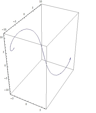
(a) The curve $r\left(s\right)$

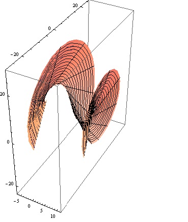
(b) A member of the family of surfaces having for $a=1,b=1$ and $c=1$ $\sigma(u)=1.$

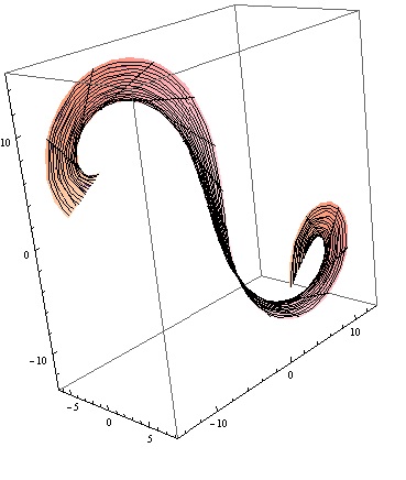
(c) A member of the family of surfaces for $a=\frac{1}{3},b=\frac{1}{5}andc=1$ $\sigma(s)=1.$

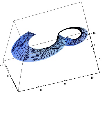
(d) A member of the family of surfaces for $a=\frac{1}{3},b=\frac{1}{5}$ and $c=1$ $\sigma(s)=u$.

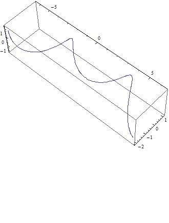
(e) The curve $r\left(s\right)$

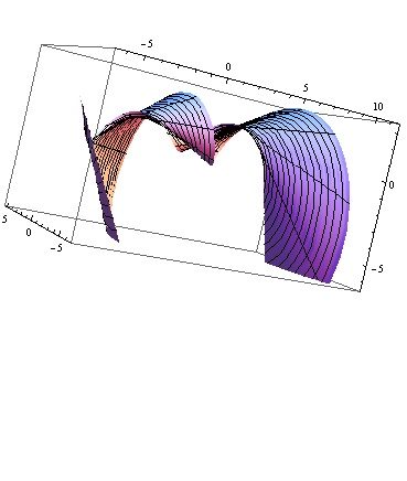
(f) A member of the family of surfaces for $a=1,b=1,c=1$ .

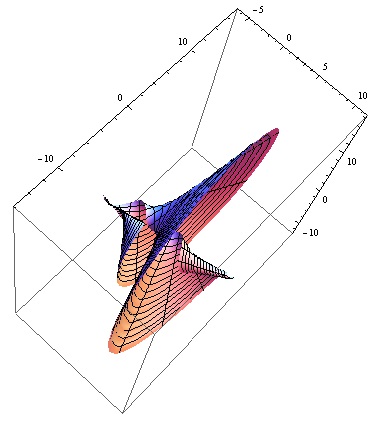
(g) A member of the family of surfaces for$a=1,b=3,c=5$.

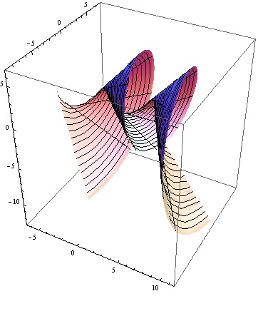
(h) A member of the family of surfaces for $a=1,b=\frac{1}{5},c=\frac{1}{10}$ .

Figure 1:

Then, we obtain the surface pencil.

If we take $l\left(s\right)=m\left(s\right)=\sigma(s)=1,n\left(s\right)=-1$ and $\lambda(s)=\frac{1}{2}$

$$X\left(v\right)=v\text{ },Y\left(v\right)=\frac{3\sqrt{7}}{8}v\text{ and }Z\left(v\right)=\frac{1}{8}v.$$

Thus, a member of this family is obtained by

$$\varphi\left(s,v\right)=r(s)+[\alpha\left(s,v\right)t\left(s\right)+\beta\left(s,v\right)n\left(s\right)+\gamma\left(s,v\right)b\left(s\right)],-2\pi\leq s\leq 2\pi,\text{ }0\leq v\leq 5.$$ (17)

Then, we plot the surface (17) in Fig 1b.

On the other hand, some control coefficients can be added to the function  $X\left(v\right),Y\left(v\right)$ and $Z\left(v\right)$ such as

$$X\left(v\right)=av\text{ },Y\left(v\right)=b\frac{3\sqrt{7}}{8}v\text{ and }Z\left(v\right)=c\frac{1}{8}v,$$

where $a,b$ and $c$ are real constants.

Considering $a=\frac{1}{3},b=\frac{1}{5}$ and $c=1,$ the plot of surface pencil between the same intervals is given by Fig.1c. We obtain the shape for taking same values of $a,b$ and $c$ and $\sigma(s)=s$ such as

$$X\left(v\right)=\frac{1}{3}v\text{ },Y\left(v\right)=\frac{1}{5}\sqrt{s^{2}-\frac{1}{64}}v\text{ and }Z\left(v\right)=\frac{1}{8}v,$$

given by Fig. 1d.

Example 3.9 Let $r(s)$ be an anti-Salkowski curve given by parametrization

$$r\left(s\right)=\left(s,\frac{16}{289}[8\sin s\sinh\frac{s}{4}-15\cos s\cosh\frac{s}{4}],-\frac{16}{289}[8\cos s\sinh\frac{s}{4}+15\sin s\cosh\frac{s}{4}]\right),$$

[1] . The shape of the curve is plotted by Fig 1e. It is easy to calculate that $\kappa=\cosh\frac{s}{4}$ and $\tau=1,$

$$t = \left(s,\frac{16}{289}[17\sin s\cosh\frac{s}{4}+\frac{17}{4}\cos s\sinh\frac{s}{4}],-\frac{16}{289}[17\cos s\cosh\frac{s}{4}-\frac{17}{4}\sin s\sinh\frac{s}{4}]\right),$$

$$n = \left(0,\cos s,\sin s\right),$$

$$b = \left(0,-\sin s,\cos s\right).$$

Then, the shape of the surface pencil is given by

$$\varphi\left(s,v\right)=r(s)+[\alpha\left(s,v\right)t\left(s\right)+\beta\left(s,v\right)n\left(s\right)+\gamma\left(s,v\right)b\left(s\right)],-2\pi\leq s\leq 2\pi,\text{ }0\leq v\leq 5.$$ (18)

If we take $\sigma(s)=\frac{1}{\left\|r^{\prime\prime}(s)\right\|}=\frac{1}{\cosh\frac{s}{4}}$ and $l\left(s\right)=m\left(s\right),n\left(s\right)=-1$, and $\lambda(s)=\frac{\sqrt{3}}{2}.$

$$X\left(v\right)=v,Y\left(v\right)=\sqrt{\frac{1}{\cosh\frac{s}{4}}-\frac{3}{4\left(\cosh\frac{s}{4}\right)^{2}}}v\text{ and }Z\left(v\right)=\frac{\sqrt{3}}{2}\cosh\frac{s}{4}v.$$

Then, we plot the surface (18) in Fig 1f. Considering the control coefficients $a=1,b=3$ and $c=5$, the shape of the surface pencil between the same intervals is plotted by Figure 1g. By taking the $a=1,b=\frac{1}{5}$ and $c=\frac{1}{10},$ the plot of surface pencil is given by Fig.1h.

References

[1] A. T. Ali, Position vectors of curves in the Galilean space
G3, Math. Bech., 64 (2012), 200-210.
[2] E. Bayram, F. Guler and E. Kasap, Parametric representation
of a surface pencil with a common asymptotic curve, Comput. Aided
Des., 44 (2012), 637-643.
[3] M. Dede, Tubular surfaces in Galilean space, Math.
Commun.,18 (2013), 209–217 .
[4] M. Dede, C. Ekici and A. C. Çöken, On the parallel
surfaces in Galilean space, Hacet. J. Math. Stat.42
(2013), 605–615 .
[5] E. Kasap and F.T. Akyildiz, Surfaces with a Common Geodesic
in Minkowski 3-space. App. Math. and Comp., 177 (2006),
260-270.
[6] M. K. Karacan,Y. Tunçer and M. Doruk, Darboux rotation
axis of the curve in Galilean and Pseudo-Galilean spaces, Journ. of
Vec. Rel.,6 (2011), 107-116.
[7] O. Kaya and M. Önder, Construction of a surface pencil
with a common special surface curve, arXiv preprint arXiv.1603.00735,
(2016).
[8] H. Kilean, On intrinsic nonlinear particle motion in compact
synchrotrons. Diss. faculty of the University Graduate School in partial
fulfillment of the requirement for the degree Doctor of Philosophy in the
Department of Physics, Indiana University, 2016.
[9] Z. Küçükarslan Yüzbaşı, On a family of
surfaces with common asymptotic curve in the Galilean Space J. Nonlinear Sci. Appl, 9 (2016), 518–523 .
[10] S. Y. Lee, Accelerator physics. World scientific,
2004.
[11] C. Y. Li, R. H. Wang and C. G. Zhu, Parametric representation
of a surface pencil with a common line of curvature. Comput. Aid.
Design. 43 (2011), 1110–1117.
[12] A. Ögrenmiş, M. Ergüt and M., Bektaş, On the
helices in the Galilean space G3. Iran. J. Sci. Tech., 31
(2007), 177–181.
[13] B. J. Pavkovic and I. Kamenarovic, The equiform differential
geometry of curves in the Galilean space G3. Glas. Mat. 22
(1907), 449-“457.
[14] O. Roschel, Die geometrie des Galileischen raumes, Forsch.
Graz, Mathematisch-Statistische Sektion, (Graz, 1985.)
[15] Z. M. Sipus, Ruled Weingarten surfaces in the Galilean
space. Period. Math. Hung. 56, (2008), 213–225.
[16] G. J. Wang, K. Tang and C.L. Tai, Parametric representation
of a surface pencil with a common spatial geodesic. Comput. Aid.
Des.,36 (2004), 447-459.
[17] I. M. Yaglom, A simple non-Euclidean geometry and its
physical basis.,Springer-Verlag, New York, 1979.