Determination of Cosmological Parameters from Gamma Ray Burst Characteristics and Afterglow Correlations

Abstract

We use the correlation relation between the energy emitted by the GRBs in their prompt phases and the X-ray afterglow fluxes, in an effort to constrain cosmological parameters and aiming to construct a Hubble diagram at high redshifts, i.e. beyond those found with Type Ia supernovae.

We use a sample of 126 Swift GRBs, that we have selected among more than 800 long bursts observed until April 2015. The selection is based on a few observational constraints: GRB flux higher than 0.4 $photons/cm^{2}/s$ in the band 15-150 keV; spectrum fitted with simple power law; redshift accurately known and given; and X-ray afterglow observed and flux measured.

The statistical method of maximum likelihood is then used to determine the best cosmological parameters ($\Omega_{M}$, $\Omega_{\Lambda}$) that give the best correlation for two relations: a) the Amati relation (between intrinsic spectral peak energy $E_{p,i}$ and the equivalent isotropic energy); b) the Dainotti relation, namely between the X-ray afterglow luminosity $L_{X}$ and the break time $T_{a}$, which is observed in the X-ray flux FX.

Although the number of GRBs with high redshifts is rather small, and despite the notable dispersion found in the data, the results we have obtained are quite encouraging and promising. The results obtained using the Amati relation are close to those obtained using the Type Ia supernovae, and they appear to indicate a universe dominated by dark energy. However, those obtained with the correlation between the break time and the X-ray afterglow luminosity is consistent with the findings of the WMAP study of the cosmic microwave background radiation, and they seem to indicate a de Sitter-Einstein universe dominated by matter.

Keywords gamma-rays: bursts, theory, observations - Methods: data analysis, statistical, chi-square, maximum likelihood

1 Introduction

Gamma-ray bursts (GRBs) are the most powerful explosions in the universe, and they occur in galaxies that can be at the farthest reaches of the (observable) universe. They have so far been observed with redshifts up to z = 9.4, with hopes of reaching z = 20 with future satellite detectors, qualifying them as potential cosmological probes. Although GRBs are not standard candles, the discovery of several luminosity and energy correlations opened a new window of investigation in which GRBs could be used to probe cosmological models and cosmological issues, like the star formation rate.

Two GRB luminosity correlations were discovered in 2000. The first is a correlation between a burst’s luminosity and the time lag between the arrival of hard and soft photons in the burst (Norris et al., 2000). The second is a correlation between a burst’s luminosity and its “spikiness” or variability (Fenimore and Ramirez-Ruiz, 2000). These two correlations were then used to create a GRB Hubble diagram (Schaefer, 2003). Other luminosity and energy correlations were soon discovered, such as: the Amati relation (Amati et al., 2002; Amati, 2006; Amati et al., 2008, 2009) which relates the intrinsic spectral peak energy, $E_{p,i}$, to the equivalent isotropic energy, $E_{iso}$; the Yonetoku relation (Yonetoku et al., 2004) which is a correlation between $E_{p,i}$ and the isotropic peak luminosity, $L_{iso}$; the Ghirlanda relation (Ghirlanda et al., 2004, 2006, 2010) which is a correlation between $E_{p,i}$ and the collimation corrected energy $E_{\gamma}$ ; and the Liang-Zhang relation (Liang and Zhang, 2005) which relates $E_{iso}$ to both $E_{p,i}$ and the break time of the optical afterglow light curves, $T_{a}$.

Early attempts to use GRB correlations to constrain cosmological parameters, such as the matter density parameter $\Omega_{M}$, faced several problems (Dai et al., 2004; Azzam and Alothman, 2006a, b). The first problem was the scatter in the correlations, which made it difficult to pin down the cosmological parameters. The second was the circularity problem, which refers to the fact that in order to calibrate the luminosity and energy correlations, one must assume a cosmological model in the first place. The third problem was the paucity of data points with the required input parameters, like the redshift and the spectral peak energy. For a detailed discussion of these issues, the reader is referred to the recent review by Amati and Della Valle (2013) and the detailed study by Dainotti et al. (2013b) who clearly demonstrate the importance of taking proper account of the circularity problem, which could, otherwise, affect the evaluation of the cosmological parameters by 10 to 13%.

In recent years, a revived interest in GRB cosmology has taken place, perhaps due to the new abundance of high quality data. For instance, Petrosian et al. (2015) investigated the cosmological evolution of a sample of 200 Swift bursts and utilized the results they obtained to put constraints on the star formation rate. Another recent study (Wang et al., 2015, 2016) provides a thorough investigation of how GRBs can be employed to constrain cosmological parameters, dark energy, the star formation rate, the pre-galactic metal enrichment, and the first stars (Totani, 1997; Wijers et al., 1998; Mao and Mo, 1998; Mao, 2010; Porciani and Madau, 2001; Natarajan et al., 2005; Hopkins and Beacom, 2006; Jakobsson et al., 2006; Dermer, 2007; Daigne and Mochkovitch, 2007; Coward, 2007; Yüksel and Kistler, 2007; Kistler et al., 2008; Dainotti et al., 2015b).

In this paper, we use a sample of 126 Swift GRBs to investigate the correlation between the energy emitted by GRBs in their prompt phase and their X-ray afterglow fluxes. GRB luminosity correlations necessarily include cosmological parameters through the dependence of the luminosity on the burst’s distance. The goal is to utilize the correlation between burst parameters to infer the best distance function, thus constraining the cosmological parameters and creating a Hubble diagram at redshifts that go beyond those found in Type Ia supernovae.

2 Data Preparation

The data for the prompt gamma portion was collected fromthe two official NASA/Swift websites, . For the X-ray part of each burst, we used the data published by the Swift public website (Evans et al., 2009).

Until 25.04.2015, Swift/BAT had observed 304 GRBs with determined redshift. These bursts include 184 ones with an X-ray counterpart observed by Swift/XRT. We eliminated two GRBs, GRB060708 ($z<2.3$) and GRB090814 ($0.696\leq z\leq 2.2$) because their redshifts are given very approximately. For consistency in our calculations, we only keep bursts that have a spectrum expressed by a single power law (PL) (Dainotti et al., 2016) and whose spectral index is given by the Swift public website. According to (Sakamoto et al., 2011) the rule of $\delta_{\chi^{2}}=\chi^{2}_{PL}-\chi^{2}_{CPL}<6$ means that the CPL does not improve significantly the fit, thus the PL can be chosen as an equally good fit.

With this constraint we are left with 152 GRBs. We then add two constraints: a duration longer than two seconds, to keep only long bursts, and fluxes greater than $0.4\leavevmode\nobreak\ \mathrm{ph.cm^{-2}.s^{-1}}$ (Ghirlanda et al., 2015). Two other GRBs were eliminated due to lack of data on their X-ray fluxes, GRB120714B, GRB080330, and a third a third one, GRB131103A, because of the presence of a very intense flare at about 1000 s. In the end, we are left with a first sample of 139 GRBs.

3 Statistical correlation methods

We use the maximum likelihood method as described in (D’Agostini, 2005; Amati et al., 2008; Dainotti et al., 2013a, 2016) to determine correlation relations. The objective is to determine the parameters $m$ and $q$ when interpolating a set of $N$ data points $(x_{i},y_{i})$ by a straight line $y=m\leavevmode\nobreak\ x\leavevmode\nobreak\ +q$ with standard deviations $\sigma_{x}$ and $\sigma_{y}$. Hence, in order to determine the parameters $(m,q,\sigma_{int})$, we follow the Bayesian approach of D’Agostini (2005) by maximizing the likelihood function $\mathcal{L}(m,q,\sigma)=exp[-L(m,q,\sigma_{int})]$, such that

$$L(m,q,\sigma)=$$

$$\frac{1}{2}\sum_{i=1}^{N}\bigg{[}\leavevmode\nobreak\ ln{({\sigma_{y}^{2}+m^{2}\sigma_{x}^{2}+\sigma_{y,i}^{2}+m^{2}\sigma_{x,i}^{2}})}$$

$$+\frac{(y_{i}-mx_{i}-q)^{2}}{\sigma_{y}^{2}+m^{2}\sigma_{x}^{2}+\sigma_{y,i}^{2}+m^{2}\sigma_{x,i}^{2}}\bigg{]},$$ (1)

where $\sigma=\sqrt{\sigma_{y}^{2}+m^{2}\sigma_{x}^{2}+\sigma_{y,i}^{2}+m^{2}\sigma_{x,i}^{2}}$. $\sigma_{x}$, $\sigma_{y}$, $\sigma_{y,i}$, and $\sigma_{x,i}$ represent the standard deviations corresponding respectively to x, y, $x_{i}$ and $y_{i}$. Because the errors on x and y were unknown, D’Agostini (2005) choose $\sigma_{x}=0$ and set $\sigma_{y}=\sigma_{v}$. This choice is justified by the fact that y depends on several hidden parameters, while x does not depend on any factor. This has recently been used by Wang et al. (2016) to justify the choice of $x=E_{p}$ and $y=E_{iso}$ instead of the reverse, because $E_{iso}$ depends on the cosmological parameters.

In this work, since we know neither $\sigma_{x}$ nor $\sigma_{y}$ we replace $m^{2}\sigma_{x}^{2}+\sigma_{y}^{2}$ by $\sigma_{int}$, noting that the latter is called extrinsic scatter by (Amati et al., 2008; Wang et al., 2016) and “intrinsic scatter” by (Dainotti et al., 2013a, 2016). It replaces the sum of all Gaussian errors that may affect ($x,y$) and which might come from other non-observed variabilities.

From the expression of $\sigma_{int}$, it is clear that the latter depends on the slope m times $\sigma_{int}$. but practically speaking, in the minimization procedure for the function $-\ln{\mathcal{L}}$ with respect to m and $\sigma_{int}$, the corresponding best value of $\sigma_{int}$ must be of the same order as $\sqrt{\sigma_{y,i}^{2}+m^{2}\sigma_{x,i}^{2}}$. Hence, it depends on m as long as $\sigma_{y,i}$ is not dominant. In this regard, and in the aim of minimization its value, we choose the dependent variable $y=f(x)$, which gives a slope m such that $|m|<1$.

We may refer to the work of Dainotti et al. (2015b) in order to compare the values of $\sigma_{int}$ obtained for different values of m and given in the two tables. In our work and our sample, with $y=L_{X}$ and $X=T_{a}$, we obtain $m=-1.4$ and $\sigma_{int}=0.6$. However, if we take $y=T_{a}$ and $x=L_{X}$, we get $m=-0.46$ and $\sigma_{int}=0.29$. Since smaller values of $m$ result in smaller values of $\sigma_{int}$, we choose $L_{X}$ as the $x$ variable and $T_{a}$ as the $y$ variable. This may be one of the reasons for the choices made by Amati (2003) and Ghirlanda et al. (2004) in their correlations.

We note that the maximization of likelihood function is performed on the two parameters $(m,\sigma_{int})$, because the parameter $q$, called “intercept” is obtained analytically from:

$$q = \bigg{[}\sum\frac{y_{i}-m\leavevmode\nobreak\ x_{i}}{\sigma_{int}^{2}+\sigma_{y,i}^{2}+m^{2}\sigma_{x,i}^{2}}\bigg{]}$$ (2)

$$\times \bigg{[}\sum\frac{1}{\sigma_{int}^{2}+\sigma_{y,i}^{2}+m^{2}\sigma_{x,i}^{2}}\bigg{]}^{-1},$$

for each pair $(m,\sigma_{int})$.

For comparison, and in simple cases, we shall use the $\chi^{2}$ statistical method, which is defined as follows:

$$\chi^{2}=\sum_{i=1}^{N}\frac{(y_{i}-m\leavevmode\nobreak\ x_{i}-q)^{2}}{\sigma^{2}},$$ (3)

where $\sigma=\sqrt{\sigma_{int}^{2}+\sigma_{y,i}^{2}+m\sigma_{x,i}^{2}}$.

This method has also been used by Amati and Della Valle (2013) to constrain the cosmological parameters. It gives the same results as the maximum likelihood method when the number of data points is large. Statistically, the maximum likelihood method is more reliable when the data set is small (Saporta, 2011; Martin, 2012).

4 Calculation of the energy $E_{iso,\gamma}$ of the prompt gamma emission

We calculate the total isotropic energy $E_{iso,\gamma}$ emitted by the burst during the prompt phase using the following expression (Cardone et al., 2011)

$$E_{iso,\gamma}=4\leavevmode\nobreak\ \pi D_{L}^{2}(z)\leavevmode\nobreak\ S_{b}\leavevmode\nobreak\ (1+z)^{-1},$$ (4)

where $S_{b}$ is the bolometric fluence. This quantity is related to the observed one by (Schaefer, 2007):

$$S_{b}=S\leavevmode\nobreak\ \frac{\int^{10^{4}/(1+z)}_{1/(1+z)}E\leavevmode\nobreak\ \Phi_{S}(E)dE}{\int^{E_{max}}_{E_{min}}E\leavevmode\nobreak\ \Phi_{S}(E)dE},$$ (5)

where S$(erg.cm^{-2})$ is the observed quantity corresponding to the fluence. The integral represents a correction term (Zitouni et al., 2014). $\Phi_{S}(E)$ is the mean spectral energy. $(E_{min},E_{max})$ is the energy range corresponding to the observing instrument. The energy range of Swift/BAT is (15 keV, 150 keV). $D_{L}$ is the GRB luminosity distance computed in terms of the redshift z,

$$D_{L}(z) = \frac{(1+z)c}{H_{0}\sqrt{|\Omega_{k}|}}sinn\{\sqrt{|\Omega_{k}|}F(z)\},$$ (6)

$$F(z) = \int^{z}_{0}\frac{dz^{\prime}}{\sqrt{(1+z^{\prime})^{2}(1+\Omega_{M}z^{\prime})-z^{\prime}(2+z^{\prime})\Omega_{\Lambda}}},$$

assuming a standard cosmological $\wedge CDM$ model with $\Omega_{k}=\Omega_{m}+\Omega_{\Lambda}-1$ , neglecting the radiation density given by the parameter $\Omega_{r}$. $c$ is the speed of light, $H_{0}$ is the Hubble constant at the present time. The $sinn$ function is the sin function if $\Omega_{k}>0$, corresponding to a “closed universe”, and the sinh function if $\Omega_{k}<0$, corresponding to an “open universe”. For a flat space, $\Omega_{k}=0$, thus $D_{L}$ simplifies to:

$$D_{L}(z)=\frac{(1+z)c}{H_{0}}\leavevmode\nobreak\ \int_{0}^{z}\frac{dz^{\prime}}{\sqrt{\Omega_{M}(1+z^{\prime})^{3}+\Omega_{L}}}.$$ (7)

5 Calculation of the luminosity $L_{X}(t)$ and the energy $E_{iso,XA}$ of the X-ray afterglow

The luminosity of the afterglow in the X-ray band, $L_{X}(t)$, corresponding to a time $t$ measured from the detection of the prompt emission, is given by the following expression (Sultana et al., 2012):

$$L_{X}(t)=4\leavevmode\nobreak\ \pi\leavevmode\nobreak\ D_{L}^{2}\leavevmode\nobreak\ F_{X}(0.3-10\leavevmode\nobreak\ keV,t)\times K_{c},$$ (8)

where $F_{X}(0.3-10\leavevmode\nobreak\ keV,t)$ is the flux observed at the time $t$ in the X-ray band. $K_{c}$ is the K-correction for the spectral power law obtained for each afterglow (Evans et al., 2009; Dainotti et al., 2010; D’Avanzo et al., 2012; Dainotti et al., 2016):

$$K_{c}=\frac{(\frac{10}{1+z})^{2-\Gamma}-(\frac{2}{1+z})^{2-\Gamma}}{10^{2-\Gamma}-0.3^{2-\Gamma}},$$ (9)

where $\Gamma$ is the measured spectral index. The X-ray afterglow energy is calculated by integrating over time from its first detection to its end.

$$E_{iso,XA}=\frac{4\pi D_{L}^{2}(z)}{1+z}\times K_{c}\int_{t_{1}}^{t_{2}}F_{X}(t)\leavevmode\nobreak\ dt,$$ (10)

where $t_{1}$ and $t_{2}$ are the start and end times of the X-ray afterglow.

The X-ray afterglow luminosity corresponding to a time $t$ is calculated from the observed flux at that time. In the Swift/XRT data, we find the X-ray afterglows observed at the start denoted by $F_{X,early}\leavevmode\nobreak\ \leavevmode\nobreak\ (erg/cm^{2}/s)$, those observed eleven hours later denoted by $F_{X,11}$, and those observed after 24 hours denoted by $F_{X,24}$.

6 Study of the different correlation relations

In Figure (1) we have plotted the energy $E_{iso,X}$ emitted by the X-ray afterglow against the luminosity $L_{X,early}$. $E_{iso,X}$ was calculated for a flat universe ($\Omega_{k}=0$, $\Omega_{\Lambda=0.7}$, $\Omega_{M}=0.3$, $H_{0}=70\leavevmode\nobreak\ km/s/Mpc$). Using the $\chi^{2}$ statistical method, we note that there is a good correlation between the two quantities, except for 13 bursts falling outside of the group: GRB060926, GRB060904B, GRB061110B, GRB070411, GRB070611, GRB070506, GRB080411, GRB090529, GRB090726, GRB091024, GRB100902A, GRB120909A, GRB140114A. This group is characterized by X-ray afterglow fluxes that either do not have breaks in their temporal profiles or have a hint of a break in a highly slanted plateau.

In the rest of our study, we thus limit our sample to 126 GRBs (the previous 139 minus these 13), as there is a good chance of finding a strong correlation for them.

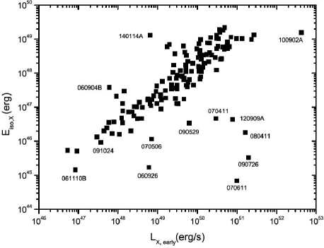
Fig. 1 : Total isotropic X-ray afterglow energy $E_{iso,X}$ against the X-ray afterglow luminosity measured very early, denoted as $L_{X,early}$. ($\Omega_{k}=0$, $\Omega_{\Lambda}=0.7$, $\Omega_{M}=0.3$, $H_{0}=70\leavevmode\nobreak\ km/s/Mpc$)

With this sample of 126 GRBs, we study the correlation between the prompt gamma emission and the X-ray afterglow. In Figure(2), we plot the isotropic X-ray afterglow energy, denoted by $E_{iso,XA}$ against the gamma isotropic emission, denoted by $E_{iso,\gamma}$. We confirm a correlation between these quantities, which are obtained using the expressions (4) and (10). The first correlation relation is expressed analytically by the equation (11). We note that we find exactly the same slope as was found by (Margutti et al., 2013). In a recent work, Zaninoni et al. (2016) find the following for long bursts: $m=0.68\pm 0.06$ and $y_{0}=16\pm 2$, corresponding to $q=-0.64\pm 0.08$. In our work, we obtain the following expression:

$$\log{(\frac{E_{iso,XA}}{erg})} = (0.74\pm 0.05)\leavevmode\nobreak\ \log{(\frac{E_{iso,\gamma}}{\leavevmode\nobreak\ erg})}$$ (11)

$$+ (12.3\pm 2.6).$$

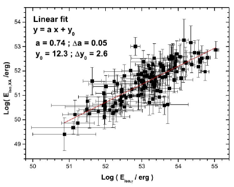
Fig. 2 : Total X-ray afterglow isotropic energy, $E_{iso,XA}$, against the prompt emission isotropic energy, $E_{iso,\gamma}$, for our 126 GRBs.

In Figure 3 we present a histogram of our 126 GRBs as a function of $\log{(E_{iso,XA}/E_{iso,\gamma})}$. We note that 67 GRBs (53 % of the sample) have a ratio $r=(E_{iso,XA}/E_{iso,\gamma})<3\%$, and 124 of them (98.4 % of the sample) have $r<30\%$. On average, we find $r=0.03^{+0.07}_{-0.02}$. Considering the error box, this result is in agreement with the ratio of $10\%$ obtained by Willingale et al. (2007) and confirmed by Dainotti et al. (2015b).

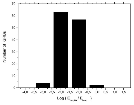
Fig. 3 : Histogram of our 126 GRBs as a function of $\log{(E_{iso,XA}/E_{iso,\Gamma})}$ with a logarithmic step equal to 1.

Aiming to confirm a correlation relation between an observed quantity and an intrinsic source quantity, we have studied the correlation relations between $L_{X}(T_{a})$, the X-ray afterglow luminosity determined at the time of the break $T_{a}$ in the temporal profile of the X-ray flux after the plateau, and the break time $T_{a}$ itself. We thus needed to determine those breaks in the X-ray flux time profiles, the latter being obtained from the Swift database Swift/XRT(Evans et al., 2009).

We should note that a correlation between $T_{a}$ and $L_{X}(T_{a})$ was found by Dainotti et al. (2008) based on a sample of 32 GRBs detected by Swift. The discovery of this relation has been the object of several updates based on newer sets of data (Dainotti et al., 2010, 2011, 2013a, 2013b, 2015a). These authors expressed $L_{X}$ as function of the break time $T_{a}/(1+z)$ in the source frame (the logarithmic variable $\log{(T_{a}/(1+z))}$. Using the maximum likelihood estimator, Dainotti et al. (2015b) get $m=-0.90^{+0.19}_{-0.17}$ and $q=51.14\pm 0.58$ on a sample of 123 GRBs. In a recent work, Dainotti et al. (2016) add a third parameter, $L_{peak}$, and infer a new correlation plane from a total sample of 176 Swift GRBs. In our work, we have preferred to keep $L_{X}$ as the independent variable and study a correlation with $T_{a}$.

Following that, we study the different possible correlations between the various intrinsic physical quantities obtained in the source’s reference frame ($L_{X}(T_{a})$, $E_{iso,XA}$, $E_{iso,\gamma}$) and the quantities observed by Swift/XRT, i.e. the break time $T_{a}$ and the X-ray flux $FX(T_{a})$. We also search for a correlation between observed flux $FX(T_{a})$ and intrinsic break time $T_{a}/(1+z)$.

This study is performed on a sample of 73 GRBs, after having kept only those bursts with an X-ray flux that has a plateau followed by a break and which can be fitted by the phenomenological model given by (Willingale et al., 2007).

In Table LABEL:tabzh1zga we list the 73 GRBs with their redshifts and their characteristic quantities which we have calculated. The temporal profiles of these bursts more or less resemble those shown in Figure 4, which presents the profile of the most recent GRB in our sample, i.e. GRB150323A.

To find the break time $T_{a}$ and its uncertainty, we use the data given in the official Swift/XRT website, which automatically treats the raw data; it classifies bursts into 5 types: (a) canonical; (b) one break, step first; (c) one break, shallow first; (d) no breaks; (o) oddball. Out of the 126 GRBs, we find 65 of type (a), 16 of type (b), 6 of type (c), 6 of type (d), and 31 of type (o). We use only the “canonical” ones (type a) and those that have a break after the X-ray flux plateau. We also add two bursts of type O, GRB100413A and GRB120729A, as their profiles are very similar to the (a) type. We thus end up with a sample of 73 bursts, given in a Table 2.

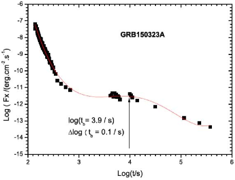
Fig. 4 : Time profile of the X-ray afterglow flux of GRB150323A.

In Figure (5) we present the relation between the X-ray flux and the break time $T_{a}$ for our sample of 73 GRBs. We confirm a correlation between the two quantities, and we express that with Equation (12). This formula does not allow us to constrain the cosmological parameters, because both quantities are observed and independent of these parameters, but it does encourage us to try to confirm a correlation between $T_{a}$ and the luminosity $L_{X}$ at $T_{a}$.

We have thus sought such a correlation in a flat universe ($\Omega_{k}=0$, $\Omega_{\Lambda}=0.7$, $\Omega_{M}=0.3$, $H_{0}=70\leavevmode\nobreak\ km/s/Mpc$). The correlation is shown graphically in Figure 6 and analytically by Equation (13). We note that these relations have rather good precisions, judging by the values of their slopes and intercepts (see the uncertainties on the power indices in Equations (12) and (13)).

$$F_{X}(T_{a}) = 10^{-7.02\pm 0.35}\leavevmode\nobreak\ T_{a}^{-1.01\pm 0.08},$$ (12)

$$\frac{T_{a}}{1+z} = 10^{25.2\pm 1.8}\leavevmode\nobreak\ \leavevmode\nobreak\ L_{X}(T_{a})^{-0.46\pm 0.04},$$ (13)

with $F_{X}$ in $(erg/cm^{2}/s)$, $T_{a}$ in seconds, and $L_{X}$ in $erg/s$. z is the redshift and $T_{a}/(1+z)$ is the break time measured in the source’s rest frame.

We may compare with the recent work of van Eerten (2014), who finds a slope of $-1.07^{+0.20}_{-0.09}$ for $F_{X}$ as a function of $T_{a}$, which is quite close to our own result.

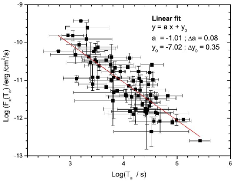
Fig. 5 : X-ray flux calculated at the break time as a function of the break time $T_{a}$ for 73 GRBs. ($\Omega_{k}=0$, $\Omega_{\Lambda}=0.7$, $\Omega_{M}=0.3$, $H_{0}=70\leavevmode\nobreak\ km/s/Mpc$)

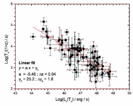
Fig. 6 : Luminosity versus break time for 73 GRBs. ($\Omega_{k}=0$, $\Omega_{\Lambda}=0.7$, $\Omega_{M}=0.3$, $H_{0}=70\leavevmode\nobreak\ km/s/Mpc$)

For that same sample of 73 GRBs we have studied the correlation between $L_{X}(T_{a})$ and the isotropic energy of the prompt gamma emission, $E_{iso,\gamma}$. We present this relation graphically in Figure(7) and analytically by Equation (14). This relation has an uncertainty of $16\%$ on the slope and about $100\%$ on the value of the intercept.

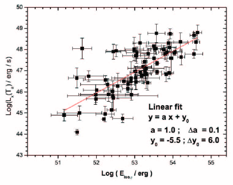
Fig. 7 : X-ray afterglow luminosity, $L_{X}$, calculated at the break time as a function of $E_{iso,\gamma}$ for our sample of 70 GRBs. ($\Omega_{k}=0$, $\Omega_{\Lambda}=0.7$, $\Omega_{M}=0.3$, $H_{0}=70\leavevmode\nobreak\ km/s/Mpc$)

$$L_{X}(T_{a})=10^{-5.5\pm 6.0}\leavevmode\nobreak\ E_{iso,\gamma}^{1.0^{\pm}0.1}.\\$$ (14)

We note that this correlation relation suffers from a very large uncertainty on the value of the intercept, therefore it cannot be used to make any convincing inferences. By contrast, despite substantial scatter, the $L_{X}-T_{a}$ plot gives an intercept with only   10 % uncertainty. From the correlations that we have sought, we thus only retain the one between the break time $T_{a}$ and the luminosity $L_{X}$ at that time, with the goal of constraining cosmological parameters.

7 Cosmological parameters derived from correlation relations

We use the maximum likelihood method as described in (D’Agostini, 2005; Amati et al., 2008; Dainotti et al., 2013a, 2016) to constrain the cosmological parameters within the standard $\Lambda CDM$ model. We should note that in this work we try to constrain the cosmological constants $\Omega_{\Lambda}$ and $\Omega_{M}$ while taking a value $H_{0}=70\leavevmode\nobreak\ km/s/Mpc$ for the Hubble constant.

7.1 Usage of the Amati Relation

We start by using the Amati relation, as presented in our previous work (Zitouni et al., 2014), in an effort to constrain the cosmological constant $\Omega_{M}$. The Amati relation is given by the following equation:

$$\frac{E_{p,i}}{keV}=K\times(\frac{E_{iso}}{10^{52}erg})^{m},$$ (15)

where $E_{p,i}$ is the energy of the burst corresponding to the peak of the flux and measured in the source’s frame, and $E_{iso}$ is the total energy emitted by the source in all space. In this work, we use data for 27 bursts to infer the constants $K$ and $m$ (Zitouni et al., 2014), and we assume a flat universe, such that $\Omega_{M}+\Omega_{\Lambda}=1$. It thus suffices to constrain one parameter to obtain the other.

Originally, the Amati relation was discovered for a flat universe, characterized by $\Omega_{k}=0$, $\Omega_{\Lambda}=0.7$, $\Omega_{M}=0.3$, $H_{0}=70\leavevmode\nobreak\ km/s/Mpc$. These values were chosen based on the results obtained from SNe Ia data. In Table 1, we present the values of the $m$ and $q$ fitting parameters found in the framework of this model.

Table 1 : Values of the slope m and intercept q. To compare with the original Amati relation, one must take $q=\log{K}-52\leavevmode\nobreak\ m$. Ref(1): Present work, Ref(2):Amati (2003), Ref(3): Ghirlanda et al. (2004). ($\Omega_{k}=0$, $\Omega_{\Lambda}=0.7$, $\Omega_{M}=0.3$, $H_{0}=70\leavevmode\nobreak\ km/s/Mpc$)

$m$	$q$	$\sigma_{int}$	Ref.
$0.37\pm 0.07$	$-15\pm 3$	$0.20\pm 0.01$	(1)
$0.35\pm 0.06$	$-16\pm 3$		(2)
$0.40\pm 0.05$	$-18.8\pm 2.7$		(3)

We stress that our novel approach consists in performing a “reverse job”, namely to search for the cosmological parameters that give the best fit, which is when the likelihood function $-\ln{\mathcal{L}}$ is minimized. The fit is not given by specific values but rather by surfaces or contours corresponding to the same values of $-\ln{\mathcal{L}}$. We vary the cosmological constant $\Omega_{M}$ numerically between 0 and 1, and determine the values presented in Table 2 for the Amati correlation relation.

Table 2 : Best values obtained for the parameters of the Amati relation using the likelihood method. Data used here consist of 27 GRBs, taken from our previous work, (Zitouni et al., 2014). Values are obtained assuming a flat universe ($\Omega_{k}=0$), with $\Omega_{M}$ varying between $0$ and $1$ and $\Omega_{\Lambda}=1-\Omega_{M}$.

parameters	$min$	$max$
m	0.32	0.37
q	-17	-15
$\sigma_{int}$	0.19	0.21
-$\ln{\mathcal{L}}$	-25	-23.5

In Figure 8, we plot the values of the function $-ln{\mathcal{L}}$ in the ($m,\Omega_{M}$) plane for a constant value of $\sigma_{int}=0.2$. Each contour is characterized by one value of $-ln{\mathcal{L}}$. We note that the best value for $-ln{\mathcal{L}}$ corresponds to low values of $\Omega_{M}\leq$.

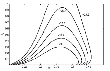
Fig. 8 : The function $-\ln{\mathcal{L}}$ in the plane ($m$ , $\Omega_{M}$), with $\sigma_{int}=0.20$ for the Amati relation obtained from the data for 27 GRBs of Swift/BAT (Zitouni et al., 2014). A contour represents the same value of $-\ln{\mathcal{L}}$ for different pairs of ($m,\Omega_{M}$). We assume a flat universe, i.e. $\Omega_{k}=0.$

In Figure 9, we plot the values of the function $-ln{\mathcal{L}}$ in the ($\sigma_{int},\Omega_{M}$) plane for a slope value of $m=0.37$. Each contour is characterized by one value of $-ln{\mathcal{L}}$. We note that the best value for $-ln{\mathcal{L}}$ corresponds to low values of $\Omega_{M}\leq 0.3$.

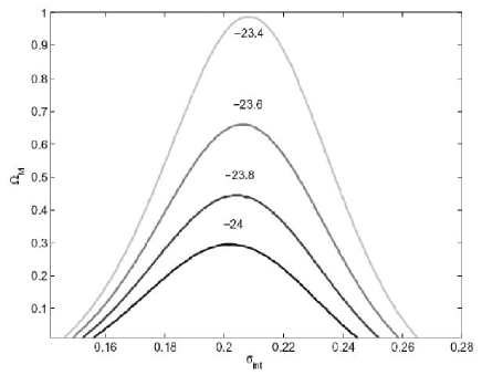
Fig. 9 : The function $-\ln{\mathcal{L}}$ in the ($\sigma_{int}$, $\Omega_{M}$) plane, with a slope $m=0.37$, for the Amati relation obtained from the data for 27 GRBs in Swift/BAT (Zitouni et al., 2014). A contour represents the same value of $-\ln{\mathcal{L}}$ for different pairs of ($\sigma_{int}$, $\Omega_{M}$). We assume a flat universe, i.e. $\Omega_{k}=0.$

In Figure 10, we plot values of the function $-ln{\mathcal{L}}$ in the plane ($m,\sigma_{int}$), assuming a constant value of $\Omega_{M}=0.3$. Each contour represents one value of $-ln{\mathcal{L}}$. We note that the best fit is for $-ln{\mathcal{L}}=-24$, which corresponds to a slope $m=0.360\pm 0.005$ and $\sigma_{int}=0.202\pm 0.004$. The intercept of the best fit is $-17\pm 1$.

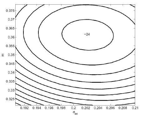
Fig. 10 : The likelihood function in the ($m,\sigma_{int}$) plane for $\Omega_{M}=0.2975$, $\Omega_{\Lambda}=0.70$ and $\Omega_{k}=0$ for the Amati relation obtained from the Swift/BAT data. The contours represent the same value of the function $-\ln{\mathcal{L}}$ obtained for different pairs ($m$ ,$\sigma_{int}$). For the innermost contour, $-\ln{\mathcal{L}}=-24$, and for each next one, 0.02 is added.

Next, we attempt to constrain the cosmological parameters $\Omega_{\Lambda}$ and $\Omega_{M}$, using the Amati relation as studied in our previous work (Zitouni et al., 2014), but in any universe (cosmological topology), that is assuming a curvature constant $\Omega_{k}=1-\Omega_{M}-\Omega_{\Lambda}$. We first determine the best values of $L=-\ln{\mathcal{L}}$, which correspond to the parameters $(m,q)$ of a straight line. In this case we vary $\Omega_{M}$ between 0 and 1.2 and $\Omega_{\Lambda}$ between 0 and 1, independently. Our results are shown graphically in Figure 11 and (with more detail) in tabular form in Table 3. The best values of the function $-\ln{\mathcal{L}}$ correspond to small values of $\Omega_{M}$ and large values of $\Omega_{\Lambda}$. In other words, the statistical method that is used tends to favor a universe dominated by dark energy if the Amati relation is correct, and not simply due to a selection effect (Nakar and Piran, 2005). For example, for $\Omega_{M}=0.0175;\Omega_{\Lambda}=0.975$ we get $m=0.3275\pm 0.0025$ and $\sigma_{int}=0.193\pm 0.0015$ with rather high precision.

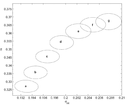
Fig. 11 : The likelihood fonction in the ($m,\sigma_{int}$) plane for different values of $\Omega_{M}$ and $\Omega_{\Lambda}$ using the Amati relation with Swift/BAT data for 27 GRBs Zitouni et al. (2014). The contours represent the values of the $-\ln{\mathcal{L}}$ function. For more information, please refer to Table (3).

Table 3 : Values of the slope $m$ and $\sigma_{int}$ for various values of $\Omega_{M}$ and $\Omega_{\Lambda}$. a, b and f represent the contours of Figure (11)

	$\Omega_{M}$	$\Omega_{\Lambda}$	$-\ln{\mathcal{L}}$
a	0.0175	0.975	-25.03
b	0.0525	0.975	-24.83
c	0.0875	0.925	-24.58
d	0.1575	0.80	-24.32
e	0.2975	0.70	-24.00
f	0.50	0.50	-23.74
g	0.10	0.997	-23.47

In Figure 12 we show the best values of the function $-\ln{\mathcal{L}}$ plotted in an $\Omega_{M}$, $\Omega_{\Lambda}$ plane diagram. On the same figure we present the contours of the values obtained by our methods for determining the cosmological parameters using the SNe Ia data. We note that it is difficult to constrain the cosmological constants using GRB correlation relations without making use of supernovae data. (Riess et al., 2004; Xu et al., 2005). The methods agree for values centered around $\Omega_{M}=0.3$ and $\Omega_{\Lambda}=0.7$. We wish to stress the fact that we did not use the Amati relation as found for the specific values of $\Omega_{M}=0.3$ and $\Omega_{\Lambda}=0.7$ in order to constrain these same parameters; that would be falling into the circularity trap(Ghirlanda et al., 2004; Dai et al., 2004).

By inverting the Amati relation and taking $E_{p,i}$ as an independent variable and $E_{iso}$ as a variable which depends on the cosmological parameters, we obtain the results shown in Figure 13. This second Amati relation is expressed by $\log{E_{iso}}=m\leavevmode\nobreak\ \log{E_{p,i}}+q$. In this case, the corresponding values of $m$, $q$, $\sigma_{int}$, and $-ln{\mathcal{L}}$ are given in Table 4. We note that the values of $\sigma_{int}$ and $-\ln{\mathcal{L}}$ are larger than those obtained with the first Amati relation. On the other hand, we note that with the inverse Amati relation, the likelihood methods tends to prefer cosmological parameters that converge toward $\Omega_{M}=0.28$ et $\Omega_{\Lambda}=0.725$.

Table 4 : Best values obtained for the parameters of the second Amati relation using the likelihood method for various values of $\Omega_{M}$ and $\Omega_{\Lambda}$. Data used here consist of 27 GRBs, taken from our previous work, (Zitouni et al., 2014).

$m$	$q$	$\sigma_{int}$	$-ln{\mathcal{L}}$
1.15	49.72	0.4216	-3.79
1.20	49.71	0.4240	-3.90
1.25	49.65	0.4264	-3.94
1.30	49.75	0.4328	-3.87
1.45	49.56	0.4512	-3.30

Our approach was rather to find the best values of the cosmological parameters that correspond to the minimum value(s) of ($-\ln{\mathcal{L}}$) and to then infer the correlation constants $m$ and $q$. This method, however, is very sensitive to the dispersion of the data. It allows one to converge on rather precise values if the data have been obtained with high precision. This procedure also allows one to verify a correlation relation by comparing with the results obtained through other methods and data (WMAP: the Wilkinson Microwave Anisotropy Probe, SN Ia).

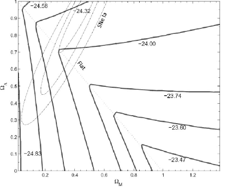
Fig. 12 : The contours of the function $-ln(\mathcal{L})$ in the $\Omega_{M},\Omega_{\Lambda}$ plane, using the Amati relation obtained from the Swift/BAT data. The contours represent the same values of the function $-\ln{\mathcal{L}}$ corresponding to $m$ and $\sigma_{int}$ given in Table 5. The dotted-line contours are the results obtained using the methods based on SNe Ia.

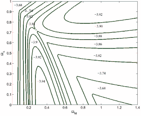
Fig. 13 : The contours of the function $-ln(\mathcal{L})$ in the $\Omega_{M},\Omega_{\Lambda}$ plane, using the inverted Amati relation obtained from the Swift/BAT data. The contours represent the same values of the function $-\ln{\mathcal{L}}$ corresponding to $m$ and $\sigma_{int}$ given in Table 4. The meeting point of the contours correspond $\Omega_{M}$= 0.28 and $\Omega_{\Lambda}$ = 0.725

7.2 Usage of the Dainotti relation

We have also attempted to use the correlation that was obtained above between the break time $T_{a}$ seen in the X-ray afterglow’s time evolution and the luminosity $L_{X}$ at that instant. For that we used the 73 bursts that we had selected. We chose this correlation because it relates an observed quantity to one which is calculated in terms of the cosmological parameters. That relation is expressed by Equation (13) and applies to a flat universe with ($\Omega_{k}=0$, $\Omega_{\Lambda}=0.7$, $\Omega_{M}=0.3$, $H_{0}=70\leavevmode\nobreak\ km/s/Mpc$). In what follows we study that relation for a more general case.

Before applying our method, let us explain what we would like to accomplish, assuming the ideal case in which our data do not suffer from any dispersion. In Figure 14, we present the case where $\Omega_{M}=0.3$. We note that our method does converge toward ($\Omega_{M}=0.3$, $\Omega_{\Lambda}=0.7)$. This is a way to check the validity of our method and the impact of the dispersion of data on our results.

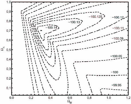
Fig. 14 : The function $-\ln{\mathcal{L}}$ in the ($\Omega_{M},\Omega_{\Lambda}$) plane for Dainotti correlation relation between the X-ray luminosity X at $T_{a}$ as a function of the break time after the temporal plateau. In the ideal case, we have used a straight line ($\log{\frac{T_{a}}{1+z}}=-0.46\log{F_{x}(T_{a})}+25.2$).

In Figure 15 we use the Dainotti correlation relation $L_{X}(T_{a})-T_{a}$ to constrain $(\Omega_{M},\Omega_{\Lambda})$ in any type of universe. We present the results as contours of specific values of $-\ln{\mathcal{L}}$. We note that the best values of this function, that is the minima of the function, are obtained for $\Omega_{\Lambda}\rightarrow 0$ and $\Omega_{M}\rightarrow 1$. In other words, Dainotti correlation relation works best in a universe dominated by matter. This result is opposite to what was obtained with the Amati relation. On the other hand, if we include the results obtained using supernovae, we obtain the same earlier results, namely values closer to $(\Omega_{M}=0.3,\Omega_{\Lambda}=0.7)$ for a flat universe.

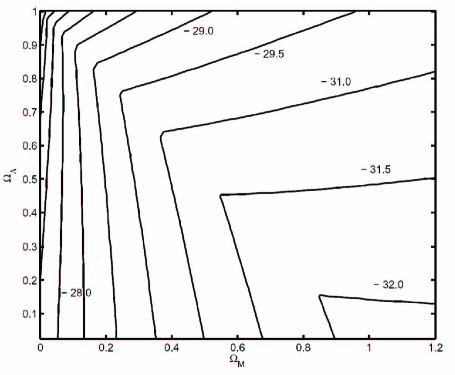
Fig. 15 : The function $-\ln{\mathcal{L}}$ in the ($\Omega_{M},\Omega_{\Lambda}$) plane using the Dainotti correlation relation between $L_{X}(T_{a})$ and $T_{a}$

In Figure 16 we show the contours for the best values of the function $-\ln{\mathcal{L}}$ in the $(m,\sigma_{int})$ plane for different values of the pair $(\Omega_{M},\Omega_{\Lambda})$. Information for each contour is given in Table 5. For example, for contour B, corresponding to $(\Omega_{M}=0.3,\Omega_{\Lambda}=0.7)$, we get $m=-0.462\pm 0.014$ and $\sigma_{int}=0.288\pm 0.012$.

Table 5 : Values for the slope $m$ and $\sigma_{int}$ for different values of $\Omega_{M}$ and $\Omega_{\Lambda}$. A and E represent the contours in Figure 16.

	$\Omega_{M}$	$\Omega_{\Lambda}$	$-\ln{\mathcal{L}}$
A	0.90	0.01	-32.02
B	0.50	0.50	-31.34
C	0.30	0.70	-30.72
D	0.10	0.90	-29.40
E	0.00	0.025	-28.55

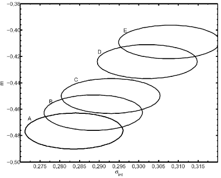
Fig. 16 : The likelihood function in the ($m$ , $\sigma_{int}$) plane for different values of $\Omega_{M}$ and $\Omega_{\Lambda}$ using the Dainotti correlation between $L_{X}(T_{a})$ and $T_{a}$ we obtained from the Swift/BAT data for 70 GRBs. The contours represent the values of the function $-\ln{\mathcal{L}}$. Further information on A and E, please refer to Table 5.

In Figure 17 we show the obtained values of $(m,\sigma_{int})$ starting from a flat space characterized by $\Omega_{M}=0.3$. We here note the ability of the likelihood method to converge to the best values of $m$ and $\sigma_{int}$.

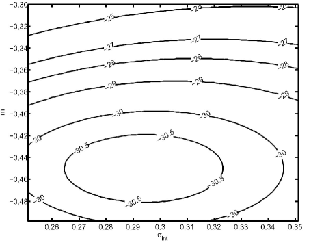
Fig. 17 : The function $-\ln{\mathcal{L}}$ in the ($\sigma_{int},m$) plane for Dainotti correlation between the X-ray luminosity and $T_{a}$ as a function of the break time after the temporal plateau. $\Omega_{M}=0.3$.

When we express the Dainotti relation by taking $Ta/(1+z)$ as an independent variable and $L_{X}$ as a variable that depends on cosmological parameters, we obtain the results shown in Figure 18. The relation that is represented there is $\log{L_{X}}=m\leavevmode\nobreak\ \log{(T_{a}/(1+z))}+q$, and we refer to it as the ‘second Dainotti relation’ to distinguish it from the first one referred to earlier. In this case, the corresponding values of $m$, $q$, $\sigma_{int}$, and $-ln{\mathcal{L}}$ are given in Table 6. We note that the values of $\sigma_{int}$ and $-ln{\mathcal{L}}$ are larger than those obtained with the first Dainotti relation while showing the same general trend.

Table 6 : Best values obtained for the parameters of the second Dainotti relation using the likelihood method for various values of $\Omega_{M}$ and $\Omega_{\Lambda}$.

$m$	$q$	$\sigma_{int}$	$-ln{\mathcal{L}}$
-1.29	51.38	0.505	5.43
-1.30	51.45	0.510	6.05
-1.31	51.53	0.520	7.07
-1.33	51.71	0.535	9.05
-1.35	51.89	0.555	11.05
-1.38	52.14	0.590	14.09
-1.41	52.37	0.615	17.21

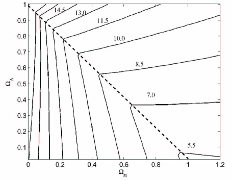
Fig. 18 : The contours of the function $-ln(\mathcal{L})$ in the $\Omega_{M},\Omega_{\Lambda}$ plane, using the second Dainotti relation obtained from the Swift/BAT data. The contours represent the same values of the function $-\ln{\mathcal{L}}$ corresponding to $m$ and $\sigma_{int}$ given in Table 6.

8 Discussion

This study was conducted to try to determine the cosmological parameters $\Omega_{\Lambda}$ and $\Omega_{M}$ by using two correlation relations: the Amati relation between $E_{p}$ and $E_{iso}$ and a Dainotti relation between $T_{a}$ and $L_{X}(T_{a})$, which we presented in the previous sections. The Amati relation has been widely used to this aim (Dai et al., 2004; Amati et al., 2008; Kodama et al., 2008; Wei et al., 2013; Wang et al., 2016). However, this relation was inferred by assuming a flat universe with $\Omega_{M}=0.3$, while some of the above-mentioned works use it as is and at the same time try to determine the cosmological parameters, which raises the issue of the circularity problem. Other works use a calibration based on the results from SN Ia for redshifts $z<1.414$ (Wang et al., 2015, 2016) , which we view as a good approach (associating the results from SNe Ia with data from GRBs).

In the present work, we have tried to constrain the cosmological parameters using the two Amati relations relation but without setting a priori values of the slope and intercept parameters m and q. The best values are those that minimize the function $L=-\ln{\mathcal{L}}$. This requirement leads to a set of values for $\Omega_{M}$ et $\Omega_{\Lambda}$ that produce contours in the plane of those cosmological variables/parameters. We find that the first Amati relation tends to favor values of $\Omega_{M}\rightarrow 0$ and $\Omega_{\Lambda}\rightarrow 1$. To relate our result with that obtained from SNe Ia, we have graphically superposed the two. On the other hand, the second Amati relation favors values of the cosmological parameters that tend to converge toward $\Omega_{M}=0.28$ and $\Omega_{\Lambda}=0.725$ in the best cases.

The second relation, Dainotti relation, which we confirmed from Swift/XRT data is between the breaking time $T_{a}$ in the time profile of the X-ray flux and the luminosity $L_{X}(T_{a})$. However, it is characterized by large dispersions of the data points around the interpolation (straight) line. For the two versions of the Dainotti relation, our statistical analysis tends to favor values of $\Omega_{M}\rightarrow 1$ and $\Omega_{\Lambda}\rightarrow 0$. By numerically reducing the dispersion of the data, the results are greatly improved and converge to a set of values of the cosmological parameters close to what is obtained by other methods

By numerically reducing the dispersion of the data, the results are greatly improved and converge to a set of values of the cosmological parameters close to what is obtained by other methods; the results are also close to those presented in Figure 14, which seems to confirm the need for “clean” data with minimal data dispersion around the straight line. We note that the Dainotti correlation has been used by several authors in an effort to constrain the cosmological parameters (Cardone et al., 2009, 2010; Dainotti et al., 2013b; Petrosian et al., 2015).

9 Conclusion

Gamma-ray bursts hold great potential as cosmological probes. This fact, however, has not yet been fully utilized, mainly because GRBs are not standard candles and partly because it has been difficult to construct plots between GRB characteristics that do not show too much scatter. The discovery and calibration of several luminosity and energy correlations has ushered in a new period of investigation in which GRBs are finally beginning to prove their worth as cosmological probes. In this paper, we tried to put limits on the values of $q$ and $m$ by utilizing the well-known Amati relation and one that was obtained by Dainotti et al. (2008) from GRB data, namely a correlation between the X-ray burst luminosity $L_{X}$ and the break time $T_{a}$ in the X-ray flux’s time profile, a correlation that we confirmed with our sample. The latter relation suffers from wide scatter, but we were able to narrow this scatter using numerical techniques. This enabled us to get reasonable values for $\Omega_{\Lambda}$ and $\Omega_{M}$ that are consistent with those obtained via other methods. A few general conclusions may be drawn from this work:

1. despite the wealth of GRB data that we now have (from Swift, Fermi, and others), the data that is plotted in the ”standard” ways (luminosity vs. time, luminosity vs energy in various bands, etc.) still shows much scatter, at least for cosmological research purposes. Either we need more data in different energy bands or we are missing some insights as to how to relate various quantities.

2. The correlation that we have confirmed(between $L_{X}$ and $T_{a}$), while far from perfect, shows that interesting perspectives can still be obtained by looking at the data from different angles.

3. Diversifying analysis approaches (maximum likelihood, chi-square minimization, iterative convergence, etc.) can yield interesting results that one may compare and contrast to reach the most robust conclusions.

4. For cosmological studies, while GRBs may certainly represent an important new angle from which to approach the determination of various parameters, combining quantities and results from different methods (SN Ia supernovae, Cosmic Microwave Background, Gamma Ray Bursts) and ensuring consistency across the board appears to be not only the best general approach but perhaps an absolutely necessary one.

In the future, we hope to pursue this new, promising avenue along the lines of the above general conclusions, in the aim of placing more stringent limits on the values of cosmological parameters, particularly by using larger data sets and GRB characteristics (energies and fluxes from various intervals and bands), which may aid in reducing the scatter in the correlation relations and thus in obtaining more precise results.

Acknowledgements

The authors gratefully acknowledge the use of the online Swift/BAT table compiled by Taka Sakamoto and Scott D. Barthelmy. We thank the referee for very useful comments, which led to significant improvements of the paper.

Table 7 : Our sample consists of 73 GRBs, of which 65 are of type (a) canonical; 6 are of type (c) one break, shallow first; 2 are of type (o): oddball. $\Gamma$ is the X-ray spectral index. The other quantities are defined in the text.

GRB	z	$\Gamma$	Log($\frac{E_{iso}}{\mathrm{erg}}$)	Log($\frac{E_{iso,XA}}{\mathrm{erg}}$)	Log($\frac{T_{a}}{\mathrm{s}})$	Log($\frac{FX(T_{a})}{\mathrm{erg/cm^{2}/s}}$)	Log($\frac{LX(T_{a})}{\mathrm{erg/s}})$
150323A a	0.593	2.06 $\pm$ 0.20	52.40 $\pm$ 0.12	50.81 $\pm$ 0.45	4.12 $\pm$ 0.35	-11.83 $\pm$ 0.19	45.15 $\pm$ 0.35
150314A c	1.758	1.85 $\pm$ 0.09	54.55 $\pm$ 0.10	52.18 $\pm$ 0.44	3.20 $\pm$ 0.14	-9.43 $\pm$ 0.02	48.69 $\pm$ 0.14
141121A a	1.470	1.93 $\pm$ 0.12	53.15 $\pm$ 0.27	51.82 $\pm$ 0.48	4.18 $\pm$ 0.06	-11.02 $\pm$ 0.12	46.92 $\pm$ 0.06
140907A a	1.210	2.01 $\pm$ 0.11	52.92 $\pm$ 0.16	51.01 $\pm$ 0.60	4.63 $\pm$ 0.25	-11.88 $\pm$ 0.02	45.86 $\pm$ 0.25
140703A a	3.140	1.83 $\pm$ 0.08	53.53 $\pm$ 0.19	52.19 $\pm$ 0.51	4.08 $\pm$ 0.14	-10.65 $\pm$ 0.05	48.03 $\pm$ 0.14
140419A a	3.956	1.87 $\pm$ 0.05	54.65 $\pm$ 0.11	52.52 $\pm$ 0.52	3.52 $\pm$ 0.36	-10.12 $\pm$ 0.14	48.81 $\pm$ 0.36
140304A a	5.283	2.02 $\pm$ 0.11	53.57 $\pm$ 0.23	52.22 $\pm$ 0.67	3.38 $\pm$ 0.44	-10.53 $\pm$ 0.53	48.77 $\pm$ 0.44
131103A a	0.599	2.19 $\pm$ 0.15	51.49 $\pm$ 0.22	50.42 $\pm$ 0.50	3.10 $\pm$ 0.47	-10.32 $\pm$ 0.24	46.65 $\pm$ 0.47
131030A a	1.293	2.10 $\pm$ 0.10	54.22 $\pm$ 0.09	52.33 $\pm$ 0.50	3.47 $\pm$ 0.38	-10.17 $\pm$ 0.15	47.65 $\pm$ 0.38
130831A a	0.479	1.79 $\pm$ 0.11	52.20 $\pm$ 0.04	50.55 $\pm$ 0.51	4.99 $\pm$ 0.07	-12.05 $\pm$ 0.14	44.72 $\pm$ 0.07
130606A a	5.913	1.87 $\pm$ 0.11	53.85 $\pm$ 0.22	52.55 $\pm$ 0.58	4.15 $\pm$ 0.43	-11.44 $\pm$ 0.28	47.88 $\pm$ 0.43
130514A a	3.600	2.06 $\pm$ 0.17	53.96 $\pm$ 0.05	52.70 $\pm$ 0.54	3.82 $\pm$ 0.76	-11.32 $\pm$ 0.69	47.60 $\pm$ 0.76
130505A a	2.270	1.92 $\pm$ 0.05	54.55 $\pm$ 0.23	52.74 $\pm$ 0.54	4.53 $\pm$ 0.21	-10.59 $\pm$ 0.05	47.80 $\pm$ 0.21
130418A c	1.218	1.69 $\pm$ 0.18	52.45 $\pm$ 0.20	51.24 $\pm$ 0.49	2.96 $\pm$ 0.35	-9.81 $\pm$ 0.24	47.90 $\pm$ 0.35
121211A a	1.023	2.07 $\pm$ 0.11	52.32 $\pm$ 0.78	51.47 $\pm$ 0.37	4.48 $\pm$ 0.33	-11.68 $\pm$ 0.17	45.88 $\pm$ 0.33
121128A a	2.200	1.98 $\pm$ 0.09	53.89 $\pm$ 0.52	51.64 $\pm$ 0.53	3.17 $\pm$ 0.14	-10.06 $\pm$ 0.09	48.32 $\pm$ 0.14
121027A a	1.773	2.37 $\pm$ 0.09	52.82 $\pm$ 0.13	53.01 $\pm$ 0.37	5.12 $\pm$ 0.12	-12.04 $\pm$ 0.04	46.16 $\pm$ 0.12
121024A a	2.298	2.01 $\pm$ 0.12	53.03 $\pm$ 0.62	51.49 $\pm$ 0.58	4.44 $\pm$ 0.56	-11.77 $\pm$ 0.40	46.66 $\pm$ 0.56
120729A o	0.800	1.88 $\pm$ 0.12	52.42 $\pm$ 0.22	50.62 $\pm$ 0.50	3.88 $\pm$ 0.12	-11.27 $\pm$ 0.02	46.03 $\pm$ 0.12
120404A a	2.876	1.90 $\pm$ 0.12	53.05 $\pm$ 0.11	51.30 $\pm$ 0.48	3.52 $\pm$ 0.37	-10.92 $\pm$ 0.32	47.71 $\pm$ 0.37
120327A a	2.810	1.76 $\pm$ 0.15	53.56 $\pm$ 0.14	51.74 $\pm$ 0.62	3.49 $\pm$ 0.27	-10.50 $\pm$ 0.04	48.05 $\pm$ 0.27
111228A a	0.716	2.04 $\pm$ 0.07	52.73 $\pm$ 0.11	51.25 $\pm$ 0.42	3.84 $\pm$ 0.13	-10.67 $\pm$ 0.17	46.50 $\pm$ 0.13
111123A a	3.152	2.56 $\pm$ 0.17	53.83 $\pm$ 0.12	52.51 $\pm$ 0.46	4.57 $\pm$ 0.35	-12.08 $\pm$ 0.08	46.84 $\pm$ 0.35
111008A a	5.000	1.94 $\pm$ 0.07	53.93 $\pm$ 0.07	52.41 $\pm$ 0.47	3.47 $\pm$ 0.24	-10.46 $\pm$ 0.10	48.75 $\pm$ 0.24
110801A a	1.858	2.05 $\pm$ 0.09	53.22 $\pm$ 0.14	52.10 $\pm$ 0.43	4.06 $\pm$ 0.39	-11.41 $\pm$ 0.18	46.80 $\pm$ 0.39
110213A a	1.460	1.96 $\pm$ 0.05	53.14 $\pm$ 0.18	51.79 $\pm$ 0.55	3.32 $\pm$ 0.41	-9.61 $\pm$ 0.02	48.32 $\pm$ 0.41
100906A a	1.727	2.03 $\pm$ 0.08	53.59 $\pm$ 0.04	52.14 $\pm$ 0.38	3.94 $\pm$ 0.10	-10.77 $\pm$ 0.17	47.36 $\pm$ 0.10
100814A a	1.440	1.89 $\pm$ 0.04	53.59 $\pm$ 0.12	52.02 $\pm$ 0.52	4.55 $\pm$ 0.11	-10.98 $\pm$ 0.20	46.93 $\pm$ 0.11
100704A a	3.600	2.12 $\pm$ 0.09	53.80 $\pm$ 0.08	52.61 $\pm$ 0.48	4.10 $\pm$ 0.28	-11.15 $\pm$ 0.24	47.79 $\pm$ 0.28
100621A a	0.542	2.30 $\pm$ 0.11	52.83 $\pm$ 0.03	51.52 $\pm$ 0.29	3.67 $\pm$ 0.41	-10.47 $\pm$ 0.26	46.38 $\pm$ 0.41
100615A a	1.398	2.38 $\pm$ 0.16	53.02 $\pm$ 0.05	51.61 $\pm$ 0.54	4.29 $\pm$ 0.18	-10.95 $\pm$ 0.09	46.97 $\pm$ 0.18
100425A a	1.755	2.17 $\pm$ 0.18	52.43 $\pm$ 1.18	50.94 $\pm$ 0.51	4.52 $\pm$ 0.70	-12.36 $\pm$ 0.39	45.81 $\pm$ 0.70
100418A a	0.624	2.27 $\pm$ 0.35	51.16 $\pm$ 0.35	50.22 $\pm$ 0.59	4.91 $\pm$ 0.28	-12.11 $\pm$ 0.06	44.90 $\pm$ 0.28
100413A o	3.900	1.96 $\pm$ 0.11	54.20 $\pm$ 0.18	52.37 $\pm$ 0.60	3.76 $\pm$ 0.42	-10.59 $\pm$ 0.27	48.37 $\pm$ 0.42
091020 a	1.710	2.09 $\pm$ 0.07	53.26 $\pm$ 0.18	51.56 $\pm$ 0.54	3.90 $\pm$ 0.20	-10.95 $\pm$ 0.00	47.18 $\pm$ 0.20
090530 a	1.266	2.04 $\pm$ 0.13	52.45 $\pm$ 0.46	50.76 $\pm$ 0.63	4.68 $\pm$ 0.58	-12.08 $\pm$ 0.32	45.71 $\pm$ 0.58
090516A a	4.109	2.09 $\pm$ 0.07	54.04 $\pm$ 0.08	52.59 $\pm$ 0.46	4.22 $\pm$ 0.10	-11.24 $\pm$ 0.14	47.83 $\pm$ 0.10
090418A a	1.608	2.03 $\pm$ 0.09	53.36 $\pm$ 0.21	51.45 $\pm$ 0.55	3.44 $\pm$ 0.21	-10.24 $\pm$ 0.02	47.81 $\pm$ 0.21
090113 c	1.749	2.25 $\pm$ 0.23	52.52 $\pm$ 0.25	50.99 $\pm$ 0.61	2.78 $\pm$ 0.28	-10.23 $\pm$ 0.02	47.94 $\pm$ 0.28
090102 c	1.547	1.77 $\pm$ 0.08	51.63 $\pm$ 0.25	51.59 $\pm$ 0.56	3.30 $\pm$ 0.49	-9.91 $\pm$ 0.44	48.06 $\pm$ 0.49
081008 a	1.968	1.98 $\pm$ 0.11	53.29 $\pm$ 0.15	51.94 $\pm$ 0.40	4.27 $\pm$ 0.24	-11.41 $\pm$ 0.03	46.85 $\pm$ 0.24
081007 a	0.529	2.10 $\pm$ 0.14	51.56 $\pm$ 0.58	50.25 $\pm$ 0.59	4.60 $\pm$ 0.33	-11.85 $\pm$ 0.10	45.00 $\pm$ 0.33
080928 a	1.692	2.14 $\pm$ 0.10	52.90 $\pm$ 0.22	51.86 $\pm$ 0.39	4.35 $\pm$ 0.15	-11.64 $\pm$ 0.05	46.48 $\pm$ 0.15
080906 a	2.000	2.00 $\pm$ 0.26	53.28 $\pm$ 0.23	51.79 $\pm$ 0.68	4.31 $\pm$ 0.48	-11.26 $\pm$ 0.28	47.02 $\pm$ 0.48
080905B a	2.374	1.86 $\pm$ 0.10	52.99 $\pm$ 0.25	51.89 $\pm$ 0.61	3.77 $\pm$ 0.56	-10.39 $\pm$ 0.34	48.03 $\pm$ 0.56
080810 a	3.350	2.12 $\pm$ 0.10	53.92 $\pm$ 0.17	52.20 $\pm$ 0.56	3.80 $\pm$ 0.21	-10.76 $\pm$ 0.01	48.10 $\pm$ 0.21
080707 a	1.230	2.07 $\pm$ 0.19	51.98 $\pm$ 0.39	50.43 $\pm$ 0.61	4.18 $\pm$ 0.47	-11.89 $\pm$ 0.17	45.88 $\pm$ 0.47
080607 a	3.036	2.03 $\pm$ 0.09	54.61 $\pm$ 0.09	52.37 $\pm$ 0.44	3.35 $\pm$ 0.37	-10.38 $\pm$ 0.16	48.35 $\pm$ 0.37
080430 a	0.767	2.04 $\pm$ 0.08	51.99 $\pm$ 0.25	50.76 $\pm$ 0.61	4.51 $\pm$ 0.17	-11.58 $\pm$ 0.11	45.67 $\pm$ 0.17
080310 a	2.427	2.09 $\pm$ 0.06	53.30 $\pm$ 0.48	52.27 $\pm$ 0.39	4.04 $\pm$ 0.11	-11.39 $\pm$ 0.15	47.12 $\pm$ 0.11
071021 a	2.452	2.13 $\pm$ 0.13	52.91 $\pm$ 0.43	51.69 $\pm$ 0.50	4.43 $\pm$ 0.78	-11.87 $\pm$ 0.96	46.65 $\pm$ 0.78
070810A c	2.170	2.17 $\pm$ 0.16	53.30 $\pm$ 0.12	50.85 $\pm$ 0.61	3.80 $\pm$ 0.71	-11.54 $\pm$ 0.66	46.86 $\pm$ 0.71
070714B a	0.920	2.07 $\pm$ 0.15	52.30 $\pm$ 0.71	50.37 $\pm$ 0.45	3.42 $\pm$ 0.27	-11.10 $\pm$ 0.09	46.35 $\pm$ 0.27
070529 a	2.500	1.98 $\pm$ 0.17	53.51 $\pm$ 0.48	51.16 $\pm$ 0.69	3.42 $\pm$ 0.54	-10.92 $\pm$ 0.35	47.59 $\pm$ 0.54
070318 a	0.836	1.97 $\pm$ 0.10	52.69 $\pm$ 0.27	50.97 $\pm$ 0.46	5.43 $\pm$ 0.19	-12.60 $\pm$ 0.03	44.75 $\pm$ 0.19
070306 a	1.497	1.94 $\pm$ 0.07	53.22 $\pm$ 0.23	51.72 $\pm$ 0.50	4.28 $\pm$ 0.16	-10.77 $\pm$ 0.14	47.19 $\pm$ 0.16
070208 c	1.165	2.20 $\pm$ 0.19	51.80 $\pm$ 0.39	50.35 $\pm$ 0.58	3.12 $\pm$ 0.25	-10.96 $\pm$ 0.09	46.75 $\pm$ 0.25
070129 a	2.338	2.28 $\pm$ 0.12	53.18 $\pm$ 0.17	52.23 $\pm$ 0.45	4.41 $\pm$ 0.22	-11.75 $\pm$ 0.22	46.76 $\pm$ 0.22
070110 a	2.352	2.09 $\pm$ 0.06	53.06 $\pm$ 0.28	51.80 $\pm$ 0.57	3.54 $\pm$ 0.27	-10.62 $\pm$ 0.12	47.85 $\pm$ 0.27
061222A a	2.088	1.93 $\pm$ 0.06	53.90 $\pm$ 0.12	52.14 $\pm$ 0.58	4.83 $\pm$ 0.27	-11.41 $\pm$ 0.13	46.90 $\pm$ 0.27
061121 a	1.314	1.90 $\pm$ 0.06	53.77 $\pm$ 0.09	52.04 $\pm$ 0.40	3.05 $\pm$ 0.20	-9.82 $\pm$ 0.14	48.00 $\pm$ 0.20
061021 a	0.346	1.99 $\pm$ 0.06	52.23 $\pm$ 0.24	50.32 $\pm$ 0.52	4.61 $\pm$ 0.37	-11.47 $\pm$ 0.15	44.95 $\pm$ 0.37
060814 a	0.840	2.12 $\pm$ 0.07	53.34 $\pm$ 0.09	51.36 $\pm$ 0.42	3.81 $\pm$ 0.36	-10.92 $\pm$ 0.05	46.43 $\pm$ 0.36
060729 a	0.540	2.02 $\pm$ 0.04	52.01 $\pm$ 0.35	51.37 $\pm$ 0.45	4.49 $\pm$ 0.06	-10.79 $\pm$ 0.20	46.09 $\pm$ 0.06
060719 a	1.532	2.57 $\pm$ 0.15	52.56 $\pm$ 0.11	50.91 $\pm$ 0.58	4.23 $\pm$ 0.61	-11.76 $\pm$ 0.41	46.27 $\pm$ 0.61
060714 a	2.710	2.04 $\pm$ 0.11	53.26 $\pm$ 0.07	51.86 $\pm$ 0.51	3.67 $\pm$ 0.35	-11.18 $\pm$ 0.05	47.44 $\pm$ 0.35
060614 a	0.130	1.90 $\pm$ 0.08	51.50 $\pm$ 0.04	50.76 $\pm$ 0.25	4.51 $\pm$ 0.14	-11.39 $\pm$ 0.12	44.09 $\pm$ 0.14
060607A a	3.082	1.61 $\pm$ 0.05	53.50 $\pm$ 0.20	52.30 $\pm$ 0.52	4.11 $\pm$ 0.05	-10.41 $\pm$ 0.13	48.17 $\pm$ 0.05
060605 a	3.800	2.02 $\pm$ 0.09	52.99 $\pm$ 0.44	51.57 $\pm$ 0.61	3.77 $\pm$ 0.32	-11.00 $\pm$ 0.06	47.96 $\pm$ 0.32
060604 a	2.136	2.17 $\pm$ 0.12	52.24 $\pm$ 0.58	51.58 $\pm$ 0.51	4.40 $\pm$ 0.20	-11.82 $\pm$ 0.11	46.57 $\pm$ 0.20
060526 a	3.210	1.91 $\pm$ 0.12	53.04 $\pm$ 0.35	52.38 $\pm$ 0.46	4.33 $\pm$ 0.26	-11.03 $\pm$ 0.17	47.71 $\pm$ 0.26
060502A a	1.510	2.03 $\pm$ 0.12	53.04 $\pm$ 0.24	51.31 $\pm$ 0.63	4.44 $\pm$ 0.36	-11.50 $\pm$ 0.06	46.48 $\pm$ 0.36
060210 a	3.910	2.08 $\pm$ 0.05	54.06 $\pm$ 0.19	52.59 $\pm$ 0.52	4.46 $\pm$ 0.17	-11.12 $\pm$ 0.07	47.90 $\pm$ 0.17

References

- Amati (2003) Amati, L.: Chinese Journal of Astronomy and Astrophysics Supplement 3, 455 (2003). astro-ph/0405318
- Amati (2006) Amati, L.: Mon. Not. R. Astron. Soc. 372, 233 (2006). doi:10.1111/j.1365-2966.2006.10840.x
- Amati and Della Valle (2013) Amati, L., Della Valle, M.: International Journal of Modern Physics D 22, 1330028 (2013). 1310.3141. doi:10.1142 /S0218271813300280
- Amati et al. (2009) Amati, L., Frontera, F., Guidorzi, C.: Astron. Astrophys. 508, 173 (2009). 0907.0384. doi:10.1051/0004-6361/200912788
- Amati et al. (2002) Amati, L., Frontera, F., Tavani, M., in’t Zand, J.J.M., Antonelli, A., Costa, E., Feroci, M., Guidorzi, C., Heise, J., Masetti, N., Montanari, E., Nicastro, L., Palazzi, E., Pian, E., Piro, L., Soffitta, P.: Astron. Astrophys. 390, 81 (2002). doi:10.1051/0004-6361:20020722
- Amati et al. (2008) Amati, L., Guidorzi, C., Frontera, F., Della Valle, M., Finelli, F., Landi, R., Montanari, E.: Mon. Not. R. Astron. Soc. 391, 577 (2008). 0805.0377. doi:10.1111/j.1365-2966.2008.13943.x
- Azzam and Alothman (2006a) Azzam, W.J., Alothman, M.J.: Advances in Space Research 38, 1303 (2006a). doi:10.1016/j.asr.2004.12.019
- Azzam and Alothman (2006b) Azzam, W.J., Alothman, M.J.: Nuovo Cimento B Serie 121, 1431 (2006b). doi:10.1393/ncb/i2007-10270-5
- Cardone et al. (2009) Cardone, V.F., Capozziello, S., Dainotti, M.G.: Mon. Not. R. Astron. Soc. 400, 775 (2009). 0901.3194
- Cardone et al. (2011) Cardone, V.F., Perillo, M., Capozziello, S.: Mon. Not. R. Astron. Soc. 417, 1672 (2011). 1105.1122
- Cardone et al. (2010) Cardone, V.F., Dainotti, M.G., Capozziello, S., Willingale, R.: Mon. Not. R. Astron. Soc. 408, 1181 (2010). 1005.0122. doi:10.1111/j.1365-2966.2010.17197.x
- Coward (2007) Coward, D.: New Astron. Rev. 51, 539 (2007). astro-ph/0702704. doi:10.1016/j.newar.2007.03.003
- D’Agostini (2005) D’Agostini, G.: ArXiv Physics e-prints (2005). physics /0511182
- Dai et al. (2004) Dai, Z.G., Liang, E.W., Xu, D.: Astrophys. J. Lett. 612, 101 (2004). astro-ph/0407497. doi:10.1086/424694
- Daigne and Mochkovitch (2007) Daigne, F., Mochkovitch, R.: Astron. Astrophys. 465, 1 (2007). 0707.0931. doi:10.1051/0004-6361:20066080
- Dainotti et al. (2008) Dainotti, M.G., Cardone, V.F., Capozziello, S.: Mon. Not. R. Astron. Soc. 391, 79 (2008). 0809.1389
- Dainotti et al. (2011) Dainotti, M.G., Ostrowski, M., Willingale, R.: Mon. Not. R. Astron. Soc. 418, 2202 (2011). 1103.1138. doi:10.1111/j.1365-2966.2011.19433.x
- Dainotti et al. (2010) Dainotti, M.G., Willingale, R., Capozziello, S., Fabrizio Cardone, V., Ostrowski, M.: Astrophys. J. Lett. 722, 215 (2010). 1009.1663. doi:10.1088/2041-8205/722/2/L215
- Dainotti et al. (2013a) Dainotti, M.G., Petrosian, V., Singal, J., Ostrowski, M.: Astrophys. J. 774, 157 (2013a). 1307.7297
- Dainotti et al. (2013b) Dainotti, M.G., Cardone, V.F., Piedipalumbo, E., Capozziello, S.: Mon. Not. R. Astron. Soc. 436, 82 (2013b). 1308.1918. doi:10.1093/mnras/stt1516
- Dainotti et al. (2015a) Dainotti, M.G., Del Vecchio, R., Shigehiro, N., Capozziello, S.: Astrophys. J. 800, 31 (2015a). 1412.3969
- Dainotti et al. (2015b) Dainotti, M., Petrosian, V., Willingale, R., O’Brien, P., Ostrowski, M., Nagataki, S.: Mon. Not. R. Astron. Soc. 451, 3898 (2015b). 1506.00702. doi:10.1093/mnras/stv1229
- Dainotti et al. (2016) Dainotti, M., Postnikov, S., Hernandez, X., Ostrowski, M.: ArXiv e-prints (2016). 1604.06840
- D’Avanzo et al. (2012) D’Avanzo, P., Salvaterra, R., Sbarufatti, B., Nava, L., Melandri, A., Bernardini, M.G., Campana, S., Covino, S., Fugazza, D., Ghirlanda, G., Ghisellini, G., Parola, V.L., Perri, M., Vergani, S.D., Tagliaferri, G.: Mon. Not. R. Astron. Soc. 425, 506 (2012). 1206.2357. doi:10.1111/j.1365-2966.2012.21489.x
- Dermer (2007) Dermer, C.D.: Astrophys. Space Sci. 309, 127 (2007). astro-ph/0610195. doi:10.1007/s10509-007-9417-8
- Evans et al. (2009) Evans, P.A., Beardmore, A.P., Page, K.L., Osborne, J.P., O’Brien, P.T., Willingale, R., Starling, R.L.C., Burrows, D.N., Godet, O., Vetere, L., Racusin, J., Goad, M.R., Wiersema, K., Angelini, L., Capalbi, M., Chincarini, G., Gehrels, N., Kennea, J.A., Margutti, R., Morris, D.C., Mountford, C.J., Pagani, C., Perri, M., Romano, P., Tanvir, N.: Mon. Not. R. Astron. Soc. 397, 1177 (2009). 0812.3662. doi:10.1111/j.1365-2966.2009.14913.x
- Fenimore and Ramirez-Ruiz (2000) Fenimore, E.E., Ramirez-Ruiz, E.: ArXiv Astrophysics e-prints (2000). astro-ph/0004176
- Ghirlanda et al. (2004) Ghirlanda, G., Ghisellini, G., Lazzati, D.: Astrophys. J. 616, 331 (2004). doi:10.1086/424913
- Ghirlanda et al. (2010) Ghirlanda, G., Nava, L., Ghisellini, G.: Astron. Astrophys. 511, 43 (2010). 0908.2807. doi:10.1051/0004-6361/200913134
- Ghirlanda et al. (2004) Ghirlanda, G., Ghisellini, G., Lazzati, D., Firmani, C.: Astrophys. J. Lett. 613, 13 (2004). astro-ph/0408350. doi:10.1086/424915
- Ghirlanda et al. (2006) Ghirlanda, G., Ghisellini, G., Firmani, C., Nava, L., Tavecchio, F., Lazzati, D.: Astron. Astrophys. 452, 839 (2006). astro-ph/0511559. doi:10.1051/0004-6361:20054544
- Ghirlanda et al. (2015) Ghirlanda, G., Salvaterra, R., Ghisellini, G., Mereghetti, S., Tagliaferri, G., Campana, S., Osborne, J.P., O’Brien, P., Tanvir, N., Willingale, D., Amati, L., Basa, S., Bernardini, M.G., Burlon, D., Covino, S., D’Avanzo, P., Frontera, F., Götz, D., Melandri, A., Nava, L., Piro, L., Vergani, S.D.: Mon. Not. R. Astron. Soc. 448, 2514 (2015). 1502.02676. doi:10.1093/mnras/stv183
- Hopkins and Beacom (2006) Hopkins, A.M., Beacom, J.F.: Astrophys. J. 651, 142 (2006). astro-ph/0601463. doi:10.1086/506610
- Jakobsson et al. (2006) Jakobsson, P., Levan, A., Fynbo, J.P.U., Priddey, R., Hjorth, J., Tanvir, N., Watson, D., Jensen, B.L., Sollerman, J., Natarajan, P., Gorosabel, J., Castro Cerón, J.M., Pedersen, K., Pursimo, T., Árnadóttir, A.S., Castro-Tirado, A.J., Davis, C.J., Deeg, H.J., Fiuza, D.A., Mikolaitis, S., Sousa, S.G.: Astron. Astrophys. 447, 897 (2006). astro-ph/0509888. doi:10.1051/0004-6361:20054287
- Kistler et al. (2008) Kistler, M.D., Yüksel, H., Beacom, J.F., Stanek, K.Z.: Astrophys. J. Lett. 673, 119 (2008). 0709.0381
- Kodama et al. (2008) Kodama, Y., Yonetoku, D., Murakami, T., Tanabe, S., Tsutsui, R., Nakamura, T.: Mon. Not. R. Astron. Soc. 391, 1 (2008). 0802.3428
- Liang and Zhang (2005) Liang, E., Zhang, B.: Astrophys. J. 633, 611 (2005). astro-ph/504404. doi:10.1086/491594
- Mao (2010) Mao, J.: Astrophys. J. 717, 140 (2010). 1005.1876
- Mao and Mo (1998) Mao, S., Mo, H.J.: Astron. Astrophys. 339, 1 (1998). astro-ph/9808342
- Margutti et al. (2013) Margutti, R., Zaninoni, E., Bernardini, M.G., Chincarini, G., Pasotti, F., Guidorzi, C., Angelini, L., Burrows, D.N., Capalbi, M., Evans, P.A., Gehrels, N., Kennea, J., Mangano, V., Moretti, A., Nousek, J., Osborne, J.P., Page, K.L., Perri, M., Racusin, J., Romano, P., Sbarufatti, B., Stafford, S., Stamatikos, M.: Mon. Not. R. Astron. Soc. 428, 729 (2013). 1203.1059. doi:10.1093/mnras/sts066
- Martin (2012) Martin, B.: Statistics for Physical Sciences: An Introduction. Academic Press, London, UK (2012)
- Nakar and Piran (2005) Nakar, E., Piran, T.: Mon. Not. R. Astron. Soc. 360, 73 (2005). astro-ph/0412232
- Natarajan et al. (2005) Natarajan, P., Albanna, B., Hjorth, J., Ramirez-Ruiz, E., Tanvir, N., Wijers, R.: Mon. Not. R. Astron. Soc. 364, 8 (2005). astro-ph/0505496. doi:10.1111/j.1745-3933.2005.00094.x
- Norris et al. (2000) Norris, J.P., Marani, G.F., Bonnell, J.T.: Astrophys. J. 534, 248 (2000). astro-ph/9903233. doi:10.1086/308725
- Petrosian et al. (2015) Petrosian, V., Kitanidis, E., Kocevski, D.: Astrophys. J. 806, 44 (2015). 1504.01414
- Porciani and Madau (2001) Porciani, C., Madau, P.: Astrophys. J. 548, 522 (2001). astro-ph/0008294. doi:10.1086/319027
- Riess et al. (2004) Riess, A.G., Strolger, L.-G., Tonry, J., Casertano, S., Ferguson, H.C., Mobasher, B., Challis, P., Filippenko, A.V., Jha, S., Li, W., Chornock, R., Kirshner, R.P., Leibundgut, B., Dickinson, M., Livio, M., Giavalisco, M., Steidel, C.C., Benítez, T., Tsvetanov, Z.: Astrophys. J. 607, 665 (2004). astro-ph/0402512. doi:10.1086/383612
- Sakamoto et al. (2011) Sakamoto, T., Barthelmy, S.D., Baumgartner, W.H., Cummings, J.R., Fenimore, E.E., Gehrels, N., Krimm, H.A., Markwardt, C.B., Palmer, D.M., Parsons, A.M., Sato, G., Stamatikos, M., Tueller, J., Ukwatta, T.N., Zhang, B.: Astrophys. J. Suppl. Ser. 195, 2 (2011). 1104.4689. doi:10.1088/0067-0049/195/1/2
- Saporta (2011) Saporta, G.: Probabilitès, Analyse des Donnèes et Statistique, 2nd edn. Editions Technip, Paris, FR (2011)
- Schaefer (2003) Schaefer, B.E.: Astrophys. J. Lett. 583, 67 (2003). astro-ph/0212445. doi:10.1086/368104
- Schaefer (2007) Schaefer, B.E.: Astrophys. J. 660, 16 (2007). astro-ph/0612285. doi:10.1086/511742
- Sultana et al. (2012) Sultana, J., Kazanas, D., Fukumura, K.: Astrophys. J. 758, 32 (2012). 1208.1680. doi:10.1088/0004-637X/758/1/32
- Totani (1997) Totani, T.: Astrophys. J. Lett. 486, 71 (1997). astro-ph/9707051. doi:10.1086/310853
- van Eerten (2014) van Eerten, H.J.: Mon. Not. R. Astron. Soc. 445, 2414 (2014). 1404.0283. doi:10.1093/mnras/stu1921
- Wang et al. (2015) Wang, F.Y., Dai, Z.G., Liang, E.W.: New Astron. Rev. 67, 1 (2015). 1504.00735. doi:10.1016/j.newar.2015.03.001
- Wang et al. (2016) Wang, J.S., Wang, F.Y., Cheng, K.S., Dai, Z.G.: Astron. Astrophys. 585, 68 (2016). 1509.08558. doi:10.1051/0004-6361/201526485
- Wei et al. (2013) Wei, J.-J., Wu, X.-F., Melia, F.: Astrophys. J. 772, 43 (2013). 1301.0894. doi:10.1088/0004-637X/772/1/43
- Wijers et al. (1998) Wijers, R.A.M.J., Bloom, J.S., Bagla, J.S., Natarajan, P.: Mon. Not. R. Astron. Soc. 294, 13 (1998). astro-ph/9708183. doi:10.1046/j.1365-8711.1998.01328.x
- Willingale et al. (2007) Willingale, R., O’Brien, P.T., Osborne, J.P., Godet, O., Page, K.L., Goad, M.R., Burrows, D.N., Zhang, B., Rol, E., Gehrels, N., Chincarini, G.: Astrophys. J. 662, 1093 (2007). astro-ph/0612031. doi:10.1086/517989
- Xu et al. (2005) Xu, D., Dai, Z.G., Liang, E.W.: Astrophys. J. 633, 603 (2005). astro-ph/0501458. doi:10.1086/466509
- Yonetoku et al. (2004) Yonetoku, D., Murakami, T., Nakamura, T., Yamazaki, R., Inoue, A.K., Ioka, K.: Astrophys. J. 609, 935 (2004). arXiv:astro-ph/0309217. doi:10.1086/421285
- Yüksel and Kistler (2007) Yüksel, H., Kistler, M.D.: Phys. Rev. D75(8) (2007). astro-ph/0610481
- Zaninoni et al. (2016) Zaninoni, E., Bernardini, M.G., Margutti, R., Amati, L.: Mon. Not. R. Astron. Soc. 455, 1375 (2016). 1510.05673
- Zitouni et al. (2014) Zitouni, H., Guessoum, N., Azzam, W.J.: Astrophys. Space Sci. 351, 267 (2014). doi:10.1007/s10509-014-1839-5