Determination of CFT central charge by the Wang-Landau algorithm

Abstract

We propose a simple method to estimate the central charge of the conformal field theory corresponding to a critical point of a two-dimensional lattice model from Monte Carlo simulations. The main idea is to use the Wang-Landau flat-histogram algorithm, which allows us to obtain the free energy of a lattice model on a torus as a function of torus radii. The central charge is calculated with a good precision from a free energy scaling at the critical point. We apply the method to the Ising, tricritical Ising (Blume-Capel), Potts and site-diluted Ising models, and also discuss estimation of conformal weights.

I Introduction

A key aspect of the modern theory of critical phenomena is the similarity hypothesis formulated a half century ago (see Kadanoff et al. (1967) for a historical review). The similarity is manifested as a ”scaling law”, determining exponents of singular behavior for some important thermodynamic quantities such as the specific heat and susceptibility. Kadanoff’s generalization of the similarity hypothesis Kadanoff (1966) inspired Wilson to apply the renormalization group approach Wilson (1971). These ideas made a breakthrough in the theory of critical phenomena Fisher (1998); Stanley (1999).

Another efficient approach is based on the conformal field theory (CFT). The scale invariance together with the homogeneity of the ground state indicates an existence of an additional symmetry at the critical point — the conformal invariance Polyakov (1970). In two dimensions, this symmetry is especially powerful since it manifests the infinite-dimensional Virasoro algebra Belavin et al. (1984a). The two-dimensional CFT provides a wealth of information about critical behavior, in particular, it makes possible to compute analytically or numerically a lot of observables such as multi-point correlation functions Di Francesco et al. (1997).

Conformal field theories are classified by the central charge $c$, that characterizes representations of the Virasoro algebra

$$\left[L_{n},L_{m}\right]=(n-m)L_{n+m}+\frac{c}{12}(n^{3}-n)\delta_{n+m,0},$$

where $L_{n,m}$ are generators of the algebra, $\delta_{n+m,0}$ is the Kronecker delta. Generally, CFT models have a small number of parameters, namely the central charge and conformal weights of the primary fields, $h_{i}$, which are the eigenvalues of the operator $L_{0}$. Conformal weights directly determine anomalous dimensions and other critical exponents, defining the universality class of the critical point.

In contrast to higher dimensions, in two dimensions critical exponents are less significant, and the central charge is the most important quantity defining the universality class. This can be seen by the example of the Ashkin-Teller model Ashkin and Teller (1943), where critical exponents depend continuously on the parameter of the model within the same symmetry class and the same value of the central charge $c=1$ Kadanoff and Brown (1979). Such a behavior is typical for models with $c\geq 1$ Zamolodchikov (1986, 1987).

Generally speaking, it is not easy to establish a correspondence between CFT with a particular value of the central charge and a symmetry class. On the one hand, internal symmetries are not fully explored even for so-called minimal models (with a finite number of Virasoro algebra modules). On the other hand, it is a priori unknown what CFT describes a critical behavior of a given lattice model, even if a symmetry class of the model is known. Such a situation is well represented, e.g., in frustrated spin systems. Critical behavior of such systems is often a subject of debate and controversy, for example, the controversy in $\mathbb{Z}_{2}\otimes SO(2)$ symmetry class discussed for three decades (see Korshunov (2006); Sorokin and Syromyatnikov (2012) for a review).

Another non-trivial example considered in this paper is the site-diluted Ising model. Using the symmetry arguments, one expects that the critical behavior is the same as in the pure Ising model with $c=1/2$. But previous investigations have given contradictory results Dotsenko and Dotsenko (1983); Shalaev (1984); Andreichenko et al. (1990); Kim and Patrascioiu (1994); Najafi (2016).

In the non-trivial cases, a determination of the central charge is a complicated and important problem. Several approaches have been proposed earlier by different authors Lauwers and Schütz (1991); Bastiaansen and Knops (1998); Feiguin et al. (2007). The first of these methods Lauwers and Schütz (1991) is based upon the deformation of the CFT minimal model by the magnetic field, so there are a lot of cases where it is not applicable. The second approach Bastiaansen and Knops (1998) requires careful simulations and precise multi-parametric numerical fitting of the conformal weights. The third method is only applicable to the one-dimensional integrable models Feiguin et al. (2007).

In this paper, we propose a more straightforward approach which does not have mentioned shortcomings. The main idea is to use the Wang-Landau flat-histogram algorithm Wang and Landau (2001), which allows to obtain the free energy of a lattice model on a torus as a function of torus radii. The central charge is calculated with a good precision from a free energy scaling at the critical point. To test our method, we apply it to several models with the well-known values of the central charge. We consider the Ising, tricritical Ising, three- and four-state Potts models. As a non-trivial case, we report our results on the site-diluted Ising model, that are presented in detail in a separate paper Belov et al. (2016).

II Theory and method

II.1 Wang-Landau algorithm

We consider lattice models formulated on regular lattices with lattice variables (usually spins) at the lattice vertices. The Wang-Landau algorithm Wang and Landau (2001); Landau and Binder (2014) simulates the energy distribution $\rho(E)=e^{g(E)}$ of the lattice model. The energy range is split in some number of intervals (which can coincide with the number of discrete energies). The algorithm starts with a random lattice configuration, an empty array of logarithms of energy densities $g(E_{1}),\dots,g(E_{n})$, an empty visitation histogram $h(E_{1}),\dots,h(E_{n})$ and some initial value (usually 1) of constant $a$. Then, one lattice site and a new value of the lattice variable at this site are chosen randomly. New state with the changed energy value is accepted with the probability $e^{g(E_{new})-g(E_{old})}$, at the same time the visitation number $h(E)$ is increased by 1 and $g(E)$ is increased by $a$. This procedure is repeated until the visitation histogram is relatively flat. Then the value of $a$ is divided by 2, the histogram is emptied and next step of the algorithm begins. Usually about 25-30 such steps are done in simulations. Having the energy distribution $\rho(E)$, the partition function is given by

$$Z=\sum_{E_{i}}\rho(E_{i})e^{-\frac{E_{i}}{T}}.$$ (1)

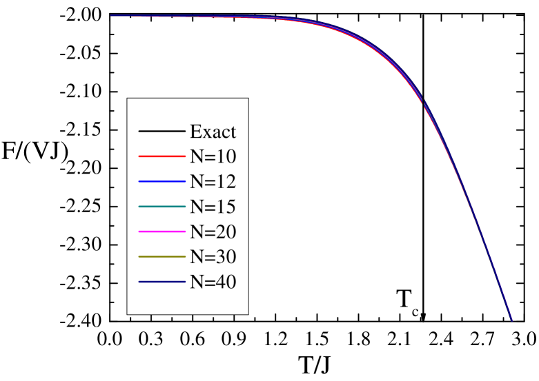
Figure 1: Free energy density in the Ising model.

Availability of the partition function in simulations is the crucial difference between the Wang-Landau and other Monte-Carlo methods, such as Metropolis Metropolis et al. (1953); Landau and Binder (2014) or Wolff algorithms Wolff (1989). Having the partition function, we can consider the free energy density

$$f(T)=-\frac{T}{V}\log Z(T),$$ (2)

where $V$ is a volume of a system. Typical thermal dependence of the free energy density is shown in Fig. 1 by the example of the Ising model on a square lattice. For comparison with the Monte Carlo results, we also show in Fig. 1 the exact result, obtained from the Onsager’s solution Onsager (1944).

II.2 Central charge

In the conformal field theory there is the well-known relation connecting the free energy $f(N)$ on an infinite cylinder of circumference $N$ with the free energy $f_{0}$ on a plane (see, for example Di Francesco et al. (1997), Chapter 5):

$$f(N)=f_{0}-\frac{\pi c}{6N^{2}}.$$ (3)

Since the central charge appears in equation (3), it can be used to extract the central charge value from the simulation data. In order to do this, we simulate a model on a torus of circumferences $N$ and $M$ to obtain the free energy density $f(N,M)$. Then we need to extrapolate the free energy value as $M\to\infty$ to calculate the free energy on a cylinder $f(N)=\lim_{M\to\infty}f(N,M)$, which is used to obtain the central charge by fitting the equation (3). To do this extrapolation, we need to know the detailed behavior of $f(N,M)$ on $M$.

Let us consider the CFT partition function on a torus of circumferences $M$ and $N$. In contrast to Bastiaansen and Knops Bastiaansen and Knops (1998) who had to study a behavior on a “skew” torus, we consider straight rectangular torus. The modular parameter of this torus is given by the ratio of two periods:

$$\tau=i\frac{M}{N}.$$ (4)

In the usual CFT quantization, one needs to choose time direction. We take it to be along the period $M$ of a torus. The Hamiltonian is the generator of time translations and is given by a sum of Virasoro generators $L_{0},\bar{L}_{0}$ Di Francesco et al. (1997):

$$H=\frac{2\pi}{N}(L_{0}+\bar{L}_{0})-\frac{\pi c}{6N},$$ (5)

the additional term with the central charge $c$ appears from the conformal mapping from a plane.

We can consider the exponent of the Hamiltonian as a row-to-row transfer matrix. Translating from row to row along the time direction $M$ times we get the partition function on the torus

$$Z=\sum_{j}\left<j\right|e^{-MH}\left|j\right>.$$ (6)

The sum here runs over states in the Hilbert space, which is in turn a direct sum of Virasoro algebra modules $V_{i}$ generated by the primary fields $\varphi_{i}$ and parametrised by the conformal weights $h_{i},\bar{h}_{i}$. A conformal field theory always contains the identity operator with the conformal weight $h_{0}=0$. The conformal weights of the other primary fields are greater then zero. We consider the minimal non-trivial conformal weight $h_{min}$ that usually lies between zero and one: $0<h_{min},\bar{h}_{\bar{m}in}<1$. We can choose the basis of Virasoro eigenstates $\left|h_{i}+m_{i},\bar{h}_{i}+\bar{m}_{i}\right>$ in the Hilbert space, where $m_{i},\bar{m}_{i}$ are positive integers:

$$\begin{array}[]{l}L_{0}\left|h_{i}+m_{i},\bar{h}_{i}+\bar{m}_{i}\right>=(h_{i}+m_{i})\left|h_{i}+m_{i},\bar{h}_{i}+\bar{m}_{i}\right>\\ \bar{L}_{0}\left|h_{i}+m_{i},\bar{h}_{i}+\bar{m}_{i}\right>=(\bar{h}_{i}+\bar{m}_{i})\left|h_{i}+m_{i},\bar{h}_{i}+\bar{m}_{i}\right>\end{array}$$ (7)

It is customary to use the parameter $q=\exp(2\pi i\tau)$. In our case of the straight rectangular torus the parameter $q$ is real, $q=\bar{q}=\exp\left(-2\pi M/N\right)$. Then for the partition function we obtain

$$\frac{Z(q)}{Z_{0}}=q^{-\frac{c}{24}}\bar{q}^{-\frac{c}{24}}\sum_{j}n_{j}q^{h_{j}+m_{j}}\bar{q}^{\bar{h}_{j}+\bar{m}_{j}}=\\ =\sum_{i,\bar{i}}{\cal M}_{i,\bar{i}}\chi_{i}(q)\bar{\chi}_{\bar{i}}(\bar{q}),$$ (8)

where $j$ runs over all states,, $n_{j}$ the multiplicity of the secondary state, $i,\bar{i}$ run over the primary states, $\chi_{i}(q)=q^{h_{i}-\frac{c}{24}}\sum_{n\geq 0}d_{i}(n)q^{n}$ is the character of the Virasoro algebra module and ${\cal M}_{i,\bar{i}}$ is the multiplicity of the representation $V_{i}\otimes\bar{V}_{\bar{i}}$. The partition function is defined up to normalization $Z_{0}$ that is interpreted as a partition function on a plane. The multiplicities $\mathcal{M}_{i,\bar{i}}$ are non-negative integers that are constrained by the modular invariance of the partition function. It is important to note that $\mathcal{M}_{0,0}=1$ since, as we have already mentioned, the CFT always contains the identity field with $h_{0}=\bar{h}_{0}=0$.

The partition function in the conformal field theory does not depend explicitly on temperature since CFT is applicable only in thermodynamic limit at critical point. Substituting equation (8) to the equation (2) at the critical point we obtain

$$f(N,M)=f_{0}-\frac{T_{c}\pi c}{6N^{2}}-\frac{T_{c}}{MN}\log\left[1+\phantom{\sum_{i\neq 0,\bar{i}\neq 0}}\right.\\ \left.\sum_{i\neq 0,\bar{i}\neq 0}\mathcal{M}_{i,\bar{i}}q^{h_{i}+\bar{h}_{\bar{i}}}\left(\sum_{n\geq 0}d_{i}(n)q^{n}\right)\left(\sum_{m\geq 0}d_{\bar{i}}(m)q^{m}\right)\right.\\ +\left.\sum_{n\geq 1}d_{0,0}(n)q^{n}\right].$$ (9)

The unit in the logarithm appears due to the identity field, and we have moved the contributions from the secondary states of the identity field $\sum_{n\geq 1}d_{0,0}(n)q^{n}$ to the right. Note that if $M\geq N$ the parameter $q=e^{-\frac{2\pi M}{N}}$ is small, so we can expand the logarithm holding only leading contributions with $q^{h_{i}}$, for $i$, such that $0<h_{i}<1$:

$$f(N,M)=f_{0}-\frac{T_{c}\pi c}{6N^{2}}-\frac{T_{c}}{MN}\left[\sum_{i\neq 0,\bar{i}\neq 0}\mathcal{M}_{i,\bar{i}}q^{h_{i}+\bar{h}_{\bar{i}}}\right].$$ (10)

This formula is the main one for our estimation of the central charge and the conformal weights.

II.3 Inaccuracies

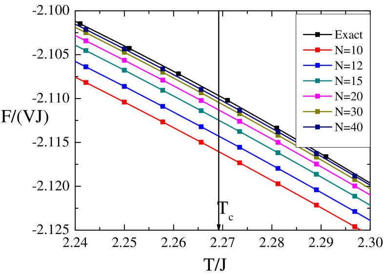
Figure 2: A thermal dependence of the free energy for different values of $N$ near the critical point.

There are several sources of inaccuracies. The first of them has the origin from the algorithm dependence on the conditions of the visitation histogram flatness and number of iterations (steps). Using 30 steps and 20% difference between a visitation number of each energy states and the average one, we estimate the free energy density with no more than $0.5\%$ inaccuracy Wang and Landau (2001); Landau and Binder (2014).

The second one follows from the estimation error of the critical temperature. But as one can see in Fig. 2, finite-size scaling corrections to the free energy depend on temperature very weakly and remain actually the same in a rather wide range of temperatures near the critical point. In practice, the critical temperature can be estimated quite precisely, so the second source of inaccuracies is insignificant compared to the rest sources.

The procedure of data fit by formula (10) may be performed in several ways depending on the accuracy of data:

1. The multiple fit procedure with the estimation of a value $f(N)$ and a few (two or more) exponents $q^{\Delta_{i,\bar{i}}}$, with $\Delta_{i,\bar{i}}=h_{i}+\bar{h}_{\bar{i}}$. Note that a multiplicity $\mathcal{M}_{i,\bar{i}}$ is small non-negative integer.

2. The multiple fit procedure with estimation of a value $f(N)$ and single exponent $q^{\Delta_{min}}$, where $\Delta_{min}$ is the minimal anomalous dimension. Such a procedure becomes correct if $M>N$ when other exponents $q^{\Delta}$ become negligible. We use this variant of the fit procedure in the current study.

3. The simple fit procedure with estimation of a value $f(N)$ using an arbitrary exponent $q^{\Delta_{r}}$, with $\Delta_{r}\in[0,1]$. Such a procedure is only accurate if $M\gg N$ (say, e.g., $M\approx 10N$), where the dependence on $\Delta_{r}$ is very weak.

4. The simplest and fastest procedure of the central charge estimation is a guess that $f(N)\approx f(N,AN)$, where $A$ is a large integer ($A\geq 10$). This procedure is valid if $M\gg N$ due to the exponential smallness of corrections.

In the table placed below, we show the estimations of the free energy value $f(N)$ with $N=10$. The exponent $\Delta$ and the central charge obtained by the last three methods for the Ising model. The uncertainty of the last decimal digit is given in brackets.

$$\begin{array}[]{c|c|c|c}\hline\cr\hline\cr&\mbox{method 2}&\mbox{method 3}&\mbox{method 4}\\ \hline\cr\Delta&0.14(3)&1&\mbox{not used}\\ f(10)&-2.1158(6)&-2.115(1)&-2.1157(6)\\ c&0.50(2)&0.46(6)&0.51(3)\\ \hline\cr\hline\cr\end{array}$$ (11)

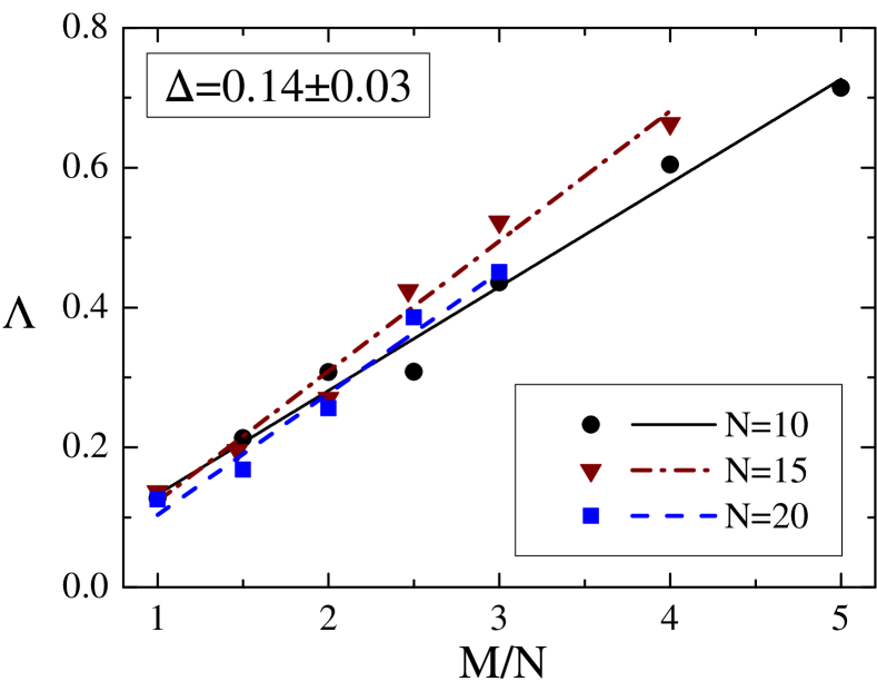
Figure 3: Estimation of the minimal conformal weight in the Ising model.

II.4 Conformal weights

The second fitting procedure described above allows us to obtain the estimation for the minimal conformal weight $h_{min}$ (or anomalous dimension $\Delta_{min}$). But it turns out that the obtained result is very sensitive to the estimated value of $f(N)$. This is especially perceptible for large torus size ratio $\frac{M}{N}\gg 1$, when the difference between $f(N)$ and $f(N,M)$ is less than the inaccuracy of the free energy value estimation. So one should exclude such lattices from a consideration. On the other hand, non-minimal exponents become perceptible for the small ratio $\frac{M}{N}\approx 1$. So we expect that a result of conformal weights estimation is far less accurate than the usual precision of a critical exponents estimation.

With our precision, we obtain an acceptable result only for the Ising model. Fig. 3 shows the results for the quantity

$$\Lambda\equiv-\frac{1}{2\pi}\ln\left(\frac{N^{2}(f(N)-f(N,M))}{T_{c}}\frac{M}{N}\right)\approx\frac{M}{N}\Delta_{min},$$ (12)

with a few values of lattice size $N$. $\Delta_{min}$ can be easily obtained by a linear fit. Then we should average over different values of $N$.

If we wanted to obtain other conformal weights we would have to do multi-parametric fit with the formula (10). However such a fit would require very precise data that could be obtained by increasing the number of algorithm iterations and enhancing the histogram flatness. This makes simulations with the Wang-Landau algorithm very time-consuming. It may be more efficient to use different approaches such as in the paper Bastiaansen and Knops (1998).

III Results

III.1 Ising model

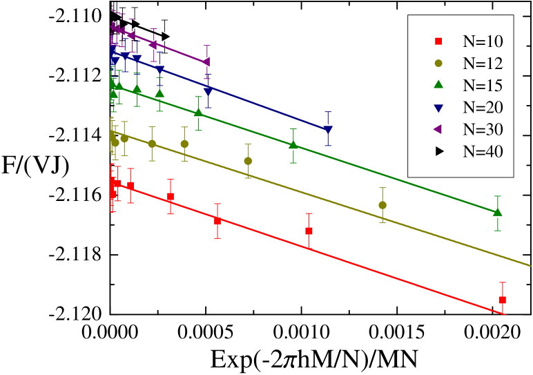
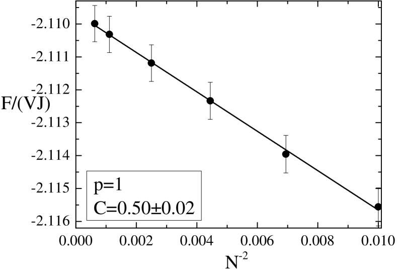
Figure 4: A finite-size scaling of the free energy $f(M,N)$ as a function of $q^{h}=e^{-2\pi hM/N}$ and $f(N)$ as a function of $N^{-2}$ in the Ising model.

The Hamiltonian of the Ising model Lenz (1920); Ising (1925) is:

$$H=-J\sum_{\left\langle i,j\right\rangle}s_{i}s_{j},\;s_{i}=\pm 1$$ (13)

where $\left\langle i,j\right\rangle$ denotes the sum over neighbouring sites of a square lattice. The quantity $J$ is the exchange energy, and we set $J=1$ to fix the energy unit.

We use two values of the critical temperature that, in fact, give the same results for the estimation of the central charge and the conformal weights. The first value is exact, obtained by Kramers-Wannier duality Kramers and Wannier (1941), whereas the second one is obtained by Monte Carlo simulation with the cluster algorithm:

$$T_{c}\mathrm{(Exact)}=\frac{2}{\ln(\sqrt{2}+1)},\quad T_{c}\mathrm{(MC)}=2.2689(3).$$ (14)

The critical point of the Ising model is described by the minimal model $\mathcal{M}(4,3)$ of the conformal field theory Belavin et al. (1984b); Di Francesco et al. (1997) with the central charge $c=\frac{1}{2}$. This model contains three primary fields with conformal dimensions $h_{r,s}$

$$h_{1,1}=0,\quad h_{2,1}=\frac{1}{16},\quad h_{1,2}=\frac{1}{2}.$$ (15)

So, the minimal non-zero dimension is $\Delta_{min}=h_{min}+\bar{h}_{min}=\frac{1}{8}$. Fitting by the method discussed we obtain the value of $\Delta_{min}=0.14\pm 0.03$ (See Fig.3), which is in agreement with CFT.

Our results on the finite-size scaling of the free energy are presented in Fig. 4. From the extrapolation of $f(N,M)$ to $M\to\infty$ we have obtained the free energy on the infinite cylinder and fitted the central charge. Our results are summarized in table 1. They are in a good agreement with the well-known values of the central charge and conformal weights obtained in CFT approach.

	Exact	This work
$c$	$\frac{1}{2}$	$0.50\pm 0.02$
$\Delta_{min}$	$\frac{1}{8}$	$0.14\pm 0.03$

Table 1: Summary of the results for the Ising model.

III.2 Site-diluted Ising model

Similar to the pure 2D Ising model, site-diluted Ising model is formulated on a lattice with magnetic sites at the lattice vertices. We performed simulations on a triangular lattice, though the critical behavior is independent of the lattice type. Each site has a spin $s=\pm 1$ or can be non-magnetic ($s=0$). Sites are magnetic with the probability $p$, so the case of $p=1$ corresponds to the Ising model. The Hamiltonian of the site-diluted model is the same as in the Ising model:

$$H=-J\sum_{\left\langle i,j\right\rangle}s_{i}s_{j},\;s_{i}=\pm 1,\mbox{or}\;0$$ (16)

where $\left\langle i,j\right\rangle$ denotes the sum over neighbouring sites of the lattice. The site-diluted Ising model has a critical point for any given value of $p$. The critical temperature changes continuously with respect to $p$.

There is a claim that the central charge should also depend on $p$ Najafi (2016). In our study we found it not to be true. Our results and discussion are presented in the separate publication Belov et al. (2016), here we present a brief summary.

We studied the model with the probabilities $p=0.8,\;0.9,\;0.95$ and performed extensive simulations.

Figure 5: Results for the central charge values in the site-diluted Ising model.

The results for the central charge are shown in Fig. 5 and in Table 2. In contrast to Ref. Najafi (2016), we see that $c$ remains close to $\frac{1}{2}$ as $p$ decreases, although the inaccuracy becomes larger.

$p$	$T_{c}$	$c$
$1$	$3.64095\ldots$	$0.50\pm 0.02$
$0.95$	$3.368\pm 0.002$	$0.47\pm 0.06$
$0.9$	$3.084\pm 0.003$	$0.48\pm 0.12$
$0.8$	$2.499\pm 0.005$	$0.54\pm 0.19$

Table 2: Summary of the results for the critical temperature and the central charge.

This result is confirmed indirectly by results of the Wolff cluster algorithm Wolff (1989); Landau and Binder (2014). The values of the critical indices for the site-diluted Ising model agree with those for the pure Ising model as it is shown in Ref.Belov et al. (2016). So, one can expect that for $0.65<p<1$ the site-diluted Ising model has the Ising-like critical behavior with $c=\frac{1}{2}$.

III.3 Tricritical Ising model

The tricritical Ising model is a short name for the tricritical point of the Blume-Capel model. The Blume-Capel model was proposed to describe the behavior of Helium Blume (1966); Balbao and de Felicio (1987); Capel (1966). It has a phase diagram with the first and second order phase transition lines and the tricritical point. We study the model on the square lattice in the tricritical point only.

The Hamilton of the model is similar to the Ising model:

$$H=-J\sum_{<i,j>}s_{i}s_{j}+D\sum_{i}s_{i}^{2},$$ (17)

where $<i,j>$ indicates nearest neighbours and spin $s_{i}$ takes values $-1,\;0,\;1$. This model is different from the site-diluted Ising model. The distribution of the non-magnetic sites is not fixed but is governed by the coupling constant $D$.

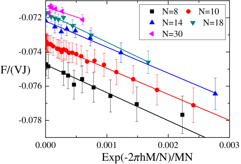
Figure 6: A finite-size scaling of the free energy $f(M,N)$ as a function of $q^{h}=e^{-2\pi hM/N}$ and $f(N)$ as a function of $N^{-2}$ in the tricritical Ising model.

The tricritical point is at da Silva et al. (2003)

$$\frac{D}{J}=1.9655,\quad T_{c}=0.610$$ (18)

It is described by the minimal model $\mathcal{M}(5,4)$ of the conformal field theory Belavin et al. (1984b); Di Francesco et al. (1997) with the central charge $c=\frac{7}{10}$.

Our results are presented in fig. 6. The estimation of the central charge by our method gives the value

$$c=0.73\pm 0.05,$$ (19)

that agrees with the exact result.

III.4 Three-state Potts model

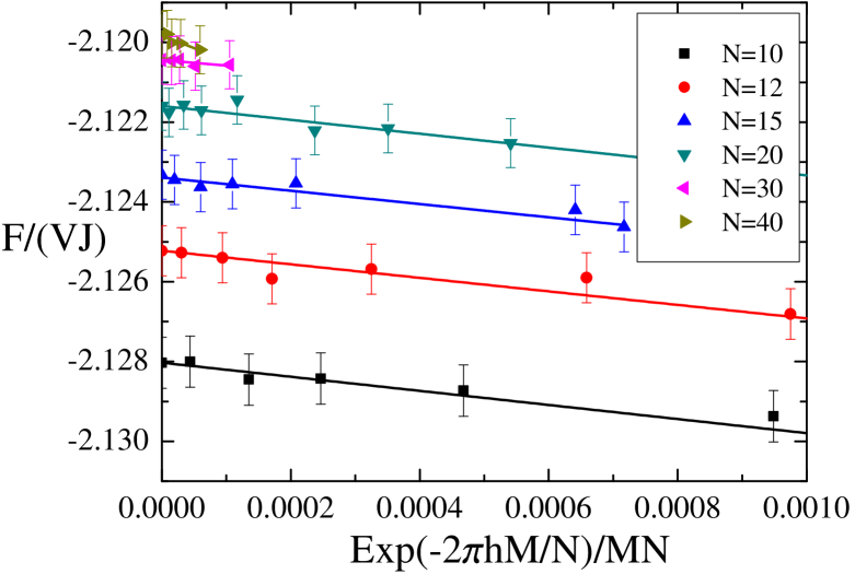
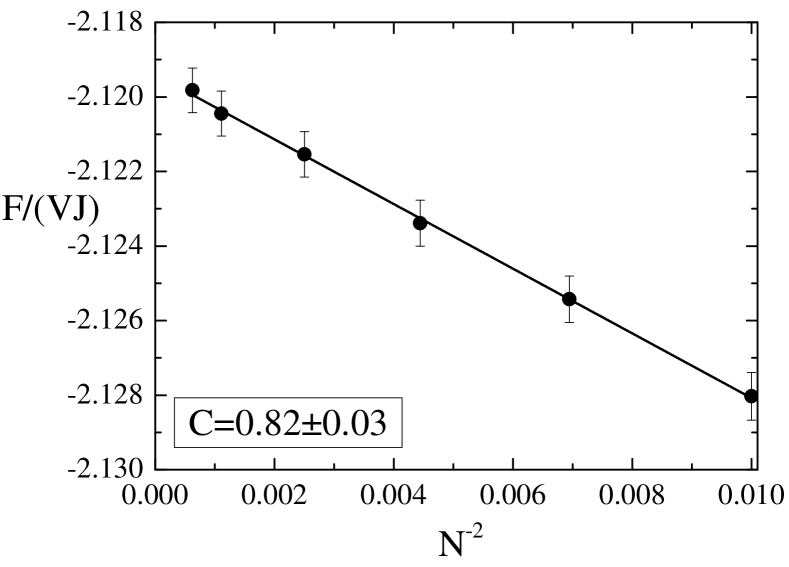
Figure 7: A finite-size scaling of the free energy $f(M,N)$ as a function of $q^{h}=e^{-2\pi hM/N}$ and $f(\infty,N)$ as a function of $N^{-2}$ in the 3-state Potts model.

The Hamilton of the (non-planar) q-state Potts model Potts (1952); Wu (1982) is

$$H=-J\sum_{<i,j>}\delta(s_{i},s_{j}),\quad s=1,\,2,\ldots,q,$$ (20)

where $\delta(s_{i},s_{j})$ is the Kronecker delta.

As in the case of the Ising model ($q=2$), we consider two values of the critical temperature: the exact Potts (1952); Wu (1982) ($q=3$) and the numerical one

$$T_{c}\mathrm{(Exact)}=\frac{2}{\ln(\sqrt{q}+1)},\quad T_{c}\mathrm{(MC)}=1.9897(3).$$ (21)

The critical point of the three-state Potts model is described by the minimal model $\mathcal{M}(6,5)$ of the CFT Dotsenko (1984); Di Francesco et al. (1997) with the central charge $c=\frac{4}{5}$. Our simulations (see fig. 7) give the value for the central charge

$$c=0.82\pm 0.03,$$ (22)

that is also in agreement with the exact value.

III.5 Four-state Potts model

Finally, we have also considered the 4-state Potts model. The critical point of it is not described by a minimal model, but this model is a particular case of the Ashkin-Teller model Ashkin and Teller (1943) with $c=1$. The Hamiltonian is given by equation (20) with $q=4$. The numerical value of the critical temperature is

$$T_{c}\mathrm{(MC)}=1.8204(3).$$ (23)

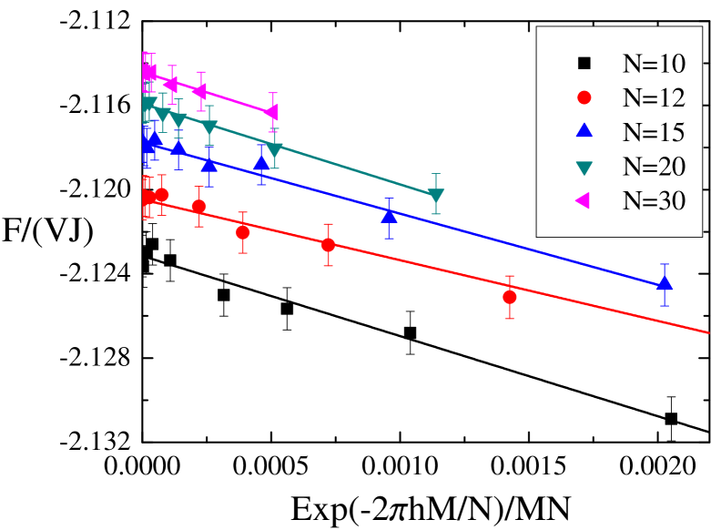
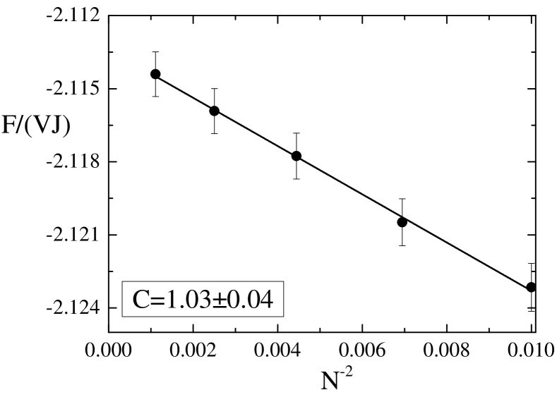
Figure 8: A finite-size scaling of the free energy $f(M,N)$ as a function of $q^{h}=e^{-2\pi hM/N}$ and $f(N)$ as a function of $N^{-2}$ in the 4-state Potts model.

Using MC simulations, we obtained the following value of the central charge

$$c=1.03\pm 0.04,$$ (24)

as it is shown in Fig. 8, that is close to 1.

Conclusion

We have presented the simple method for estimation of the central charge in the CFT corresponding to a two-dimensional lattice model at the critical point. The method is universal and can be generalized also to non-discrete spin models. We have applied the method to the Ising, site-diluted Ising, tricritical Ising, 3- and 4-state Potts models. Our numerical results on the central charge are in a perfect agreement with the analytical results for the minimal models of the CFT. We have also discussed a possibility of estimation of the conformal weights. It becomes possible if one increases the number of algorithm iterations and enhances the histogram flatness.

References

- Kadanoff et al. (1967) L. P. Kadanoff, W. Götze, D. Hamblen, R. Hecht, E. Lewis, V. V. Palciauskas, M. Rayl, J. Swift, D. Aspnes, and J. Kane, Reviews of Modern Physics 39, 395 (1967).
- Kadanoff (1966) L. Kadanoff, Physics 2, 263 (1966).
- Wilson (1971) K. G. Wilson, Physical review B 4, 3174 (1971).
- Fisher (1998) M. E. Fisher, Reviews of Modern Physics 70, 653 (1998).
- Stanley (1999) H. E. Stanley, Reviews of modern physics 71, S358 (1999).
- Polyakov (1970) A. M. Polyakov, JETP Lett. 12, 381 (1970).
- Belavin et al. (1984a) A. Belavin, A. Polyakov, and A. Zamolodchikov, Nuclear Physics 241, 333 (1984a).
- Di Francesco et al. (1997) P. Di Francesco, P. Mathieu, and D. Senechal, Conformal field theory (Springer, 1997).
- Ashkin and Teller (1943) J. Ashkin and E. Teller, Physical Review 64, 178 (1943).
- Kadanoff and Brown (1979) L. P. Kadanoff and A. C. Brown, Annals of Physics 121, 318 (1979).
- Zamolodchikov (1986) A. B. Zamolodchikov, Sov. Phys.-JETP 63, 1061 (1986).
- Zamolodchikov (1987) A. Zamolodchikov, Nuclear Physics B 285, 481 (1987).
- Korshunov (2006) S. E. Korshunov, Physics-Uspekhi 49, 225 (2006).
- Sorokin and Syromyatnikov (2012) A. Sorokin and A. Syromyatnikov, Physical Review B 85, 174404 (2012).
- Dotsenko and Dotsenko (1983) V. S. Dotsenko and V. S. Dotsenko, Advances in Physics 32, 129 (1983).
- Shalaev (1984) B. Shalaev, Fizika Tverdogo Tela 26, 3002 (1984).
- Andreichenko et al. (1990) V. Andreichenko, V. S. Dotsenko, W. Selke, and J.-S. Wang, Nuclear Physics B 344, 531 (1990).
- Kim and Patrascioiu (1994) J.-K. Kim and A. Patrascioiu, Physical review letters 72, 2785 (1994).
- Najafi (2016) M. Najafi, Physics Letters A 380, 370 (2016).
- Lauwers and Schütz (1991) P. G. Lauwers and G. Schütz, Physics Letters B 256, 491 (1991).
- Bastiaansen and Knops (1998) P. J. Bastiaansen and H. J. Knops, Physical Review E 57, 3784 (1998).
- Feiguin et al. (2007) A. Feiguin, S. Trebst, A. W. Ludwig, M. Troyer, A. Kitaev, Z. Wang, and M. H. Freedman, Physical review letters 98, 160409 (2007).
- Wang and Landau (2001) F. Wang and D. Landau, Physical review letters 86, 2050 (2001).
- Belov et al. (2016) P. A. Belov, A. A. Nazarov, and A. O. Sorokin (2016) arXiv:1611.09750 [cond-mat.stat-mech] .
- Landau and Binder (2014) D. P. Landau and K. Binder, A guide to Monte Carlo simulations in statistical physics (Cambridge university press, 2014).
- Metropolis et al. (1953) N. Metropolis, A. W. Rosenbluth, M. N. Rosenbluth, A. H. Teller, and E. Teller, The journal of chemical physics 21, 1087 (1953).
- Wolff (1989) U. Wolff, Physical Review Letters 62, 361 (1989).
- Onsager (1944) L. Onsager, Physical Review 65, 117 (1944).
- Lenz (1920) W. Lenz, Z. Phys. 21, 613 (1920).
- Ising (1925) E. Ising, Zeitschrift für Physik A Hadrons and Nuclei 31, 253 (1925).
- Kramers and Wannier (1941) H. A. Kramers and G. H. Wannier, Physical Review 60, 252 (1941).
- Belavin et al. (1984b) A. Belavin, A. Polyakov, and A. Zamolodchikov, Nuclear Physics 241, 333 (1984b).
- Blume (1966) M. Blume, Physical Review 141, 517 (1966).
- Balbao and de Felicio (1987) D. Balbao and J. D. de Felicio, Journal of Physics A: Mathematical and General 20, L207 (1987).
- Capel (1966) H. Capel, Physica 32, 966 (1966).
- da Silva et al. (2003) R. da Silva, N. A. Alves, and J. D. de Felicio, Physical Review E 67, 057102 (2003).
- Potts (1952) R. B. Potts, in Mathematical proceedings of the cambridge philosophical society, Vol. 48 (Cambridge Univ Press, 1952) pp. 106–109.
- Wu (1982) F.-Y. Wu, Reviews of modern physics 54, 235 (1982).
- Dotsenko (1984) V. S. Dotsenko, Nuclear Physics B 235, 54 (1984).