Unitary dynamics of strongly-interacting Bose gases
with time-dependent variational Monte Carlo in continuous space

Abstract

We introduce time-dependent variational Monte Carlo for continuous-space Bose gases. Our approach is based on the systematic expansion of the many-body wave-function in terms of multi-body correlations and is essentially exact up to adaptive truncation. The method is benchmarked by comparison to exact Bethe-ansatz or existing numerical results for the integrable Lieb-Liniger model. We first show that the many-body wave-function achieves high precision for ground-state properties, including energy and first-order as well as second-order correlation functions. Then, we study the out-of-equilibrium, unitary dynamics induced by a quantum quench in the interaction strength. Our time-dependent variational Monte Carlo results are benchmarked by comparison to exact Bethe ansatz results available for a small number of particles, and also compared to quench action results available for non-interacting initial states. Moreover, our approach allows us to study large particle numbers and general quench protocols, previously inaccessible beyond the mean-field level. Our results suggest that it is possible to find correlated initial states for which the long-term dynamics of local density fluctuations is close to the predictions of a simple Boltzmann ensemble.

I Introduction

The study of equilibration and thermalization properties of complex many-body systems is of fundamental interest for many areas of physics and natural sciences Nature Physics Insight on Non-equilibrium physics (2015). For systems governed by classical physics, an exact solution of Newton’s equations of motion is often numerically feasible, using for instance molecular-dynamics simulations. For quantum systems, the mathematical structure of the time-dependent Schrödinger equation is instead fundamentally more involved. Quantum Monte Carlo algorithms, the de facto tool for simulating quantum many-body systems at thermal equilibrium Ceperley (1995); Pollet (2012); Plisson et al. (2011), cannot be directly used to study time-dependent unitary dynamics. Out-of-equilibrium properties are then often treated on the basis of approximations drastically simplifying the microscopic physics. Irreversibility is either enforced with an explicit breaking of unitarity, e.g. within the quantum Boltzmann approach, or the dynamics is reduced to mean-field description using time-dependent Hartree-Fock and Gross-Pitaevskii approaches. Although these approaches may qualitatively describe thermalization Berloff and Svistunov (2002); Navon et al. (2016), their range of validity cannot be assessed because genuine quantum correlations and entanglement are ignored.

For specific systems, exact dynamical results can be derived. This is the case for integrable 1D models, for which Bethe ansatz (BA) solutions exist Gaudin (1983). However, also in this case many open questions still persist. For example, the exact evaluation of correlation functions for out-of-equilibrium dynamics is at present an unsolved problem. As a result, despite important theoretical and experimental progress Caux and Konik (2012); Caux and Essler (2013a); Collura et al. (2013); Trotzky et al. (2012); Langen et al. (2013); Greif et al. (2015); Gring et al. (2012); Cominotti et al. (2014), a complete picture of thermalization (or its absence), e.g. based on general quench protocols Calabrese and Cardy (2006), is still missing.

Numerical methods for strongly-interacting systems face important challenges as well. Numerical Renormalization Group (NRG) and Density-Matrix Renormalization Group (DMRG) approaches provide an essentially exact description of arbitrary 1D lattice systems in- and out-of-equilibrium White (1992); White and Feiguin (2004); Daley et al. (2004); Anders and Schiller (2005), but they have less predictive power when applied to continuos-space systems. On one hand, multi-scale extensions of the DMRG optimization scheme to the limit of continuous-space lattices Dolfi et al. (2012) are so-far limited to relatively small system sizes Dolfi et al. (2015). On the other hand, efficient ground-state optimization schemes for continuous quantum field matrix product states (c-MPS) Verstraete and Cirac (2010) have been introduced only very recently Ganahl et al. (2016), and applications to quantum dynamics are still to be realized. A further formidable challenge is the efficient extension of these approaches to higher dimensions, which is a fundamentally hard problem.

Another class of methods for strongly-interacting systems is based on variational Monte Carlo (VMC), combining highly-entangled variational states with robust stochastic optimization schemes Umrigar et al. (2007). Such approaches have been successfully applied to the description of continuous quantum systems, in any dimension and not only in 1D Holzmann et al. (2006); Taddei et al. (2015). More recently, out-of-equilibrium dynamics has become accessible with the extension of these methods to real-time unitary dynamics, within time-dependent variational Monte Carlo (t-VMC) Carleo et al. (2012, 2014). So far, the t-VMC approach has been developed for lattice systems with bosonic Carleo et al. (2012, 2014), spin Cevolani et al. (2015); Blaß and Rieger (2016); Carleo and Troyer (2017), and fermionic Ido et al. (2015) statistics, yielding a description of dynamical properties with an accuracy often comparable with MPS-based approaches.

In this Paper, we extend t-VMC to access dynamical properties of interacting quantum systems in continuous space. Our approach is based on a systematic expansion of the wave function in terms of few-body Jastrow correlation functions. Using the 1D Lieb-Liniger model as a test case, we first show that the inclusion of high-order correlations allows us to systematically approach the exact BA ground state energy. Our results improve by orders of magnitude on previously published VMC and c-MPS results, and are in line with latest state-of-the-art developments in the field. We further compute single-body and pair correlation functions, hardly accessible by current BA methods. We then calculate the time evolution of the contact pair correlation function following a quench in the interaction strength. For the non-interacting initial state, we benchmark our results to exact BA calculations available for a small number of bosons and further compare to the quench action approach for large systems approaching the thermodynamic limit. We finally apply our method to the study of general quenches from arbitrary initial states, for which no exact results in the thermodynamic limit are currently available.

II Method

II.1 Expansion of the Many-Body Wave-Function

Consider a non-relativistic quantum system of $N$ identical bosons in $d$ dimensions, and governed by the first-quantization Hamiltonian

$$\mathcal{H} = -\frac{1}{2}\sum_{i=1}^{N}\nabla_{i}^{2}+\sum_{i=1}^{N}v_{1}(\vec{x}_{i})+\frac{1}{2}\sum_{i\neq j}v_{2}(\vec{x}_{i},\vec{x}_{j}),$$ (1)

where $v_{1}(\vec{x})$ and $v_{2}(\vec{x},\vec{y})$ are, respectively, a one-body external potential and a pair-wise inter-particle interaction . Without loss of generality, a time-dependent $N$-body state can be written as $\Phi(\mathbf{X},t)=\exp\left[U(\mathbf{X};t)\right]$, where $\mathbf{X}=\vec{x}_{1},\vec{x}_{2}\dots\vec{x}_{N}$ is the ensemble of particle positions and $U$ is a complex-valued function of the $N$-particle coordinates, $\mathbb{R}^{N\times d}\rightarrow\mathbb{C}$. Since the Hamiltonian (1) contains only two-body interactions, it is expected that an expansion of $U$ in terms of few-body Jastrow functions containing at most $m$-body terms, rapidly converges towards the exact solution. Truncating this expansion up to a certain order $M\leq N$, leads to the Bijl-Dingle-Jastrow-Feenberg expansion Bijl (1940); Dingle (1949); Jastrow (1955); Feenberg (1969)

$$U^{(M)}(\mathbf{X};t)=\sum_{i=1}u_{1}(\vec{x}_{i};t)+\frac{1}{2!}\sum_{i\neq j}u_{2}(\vec{x}_{i},\vec{x}_{j};t)+\\ +\dots\frac{1}{M!}\sum_{i_{1}\neq i_{2}\neq\dots i_{M}}u_{M}(\vec{x}_{i_{1}},\vec{x}_{i_{2}}\dots\vec{x}_{i_{M}};t),$$ (2)

where $u_{m}(\mathbf{r};t)$ are functions of $m$ particle coordinates, $\mathbf{r}=\vec{x}_{i_{1}},\vec{x}_{i_{2}}\dots\vec{x}_{i_{m}}$, and of the time $t$. A global constraint on the function $U(\mathbf{X},t)$ is given by particle statistics. In the bosonic case, we demand that $U(\vec{x}_{1},\vec{x}_{2}\dots\vec{x}_{N})=U(\vec{x}_{\sigma(1)},\vec{x}_{\sigma(2)}\dots\vec{x}_{\sigma(N)})$, for all particle permutations $\sigma$. In general, the functions $u_{m}(\mathbf{r};t)$ can have an arbitrarily complex dependence on the $m$ particle coordinates, which can prove problematic for practical applications. Nonetheless, a simplified functional dependence can often be imposed, resulting from the two-body character of the interactions in the original Hamiltonian. For $m\geq 3$, $u_{m}(\mathbf{r};t)$ can be conveniently factorized in terms of general two-particle vector and tensor functions following Ref. Holzmann et al. (2006). Details of this approach and the present implementation are presented in Appendix A and F.

An appealing property of the many-body expansion (2) is that it is able to describe intrinsically non-local correlations in space. For instance the two-body $u_{2}(\vec{x}_{i},\vec{x}_{j};t)$, as well as any $m$-body function $u_{m}(\mathbf{r};t)$, can be long range in the particle separation $\left|\vec{x}_{i}-\vec{x}_{j}\right|$. This non-local spatial structure allows for a correct description of gapless phases, where a two-body expansion may already capture all the universal features, in the sense of the renormalization group approach Kane et al. (1991). This is in contrast with the MPS decomposition of the wave-function, which is intrinsically local in space.

II.2 Time-Dependent Variational Monte Carlo

The time evolution of the variational state (2) is entirely determined by the time-dependence of the Jastrow functions $u_{m}(\mathbf{r};t)$. In order to establish optimal equations of motion for the variational parameters, we start noticing that the functional derivative of $U(\mathbf{X};t)$ with respect to the variational, complex-valued, Jastrow functions $u_{m}(\mathbf{r};t)$,

$$\frac{\delta U(\mathbf{X};t)}{\delta u_{m}(\mathbf{r};t)} \equiv\rho_{m}(\mathbf{r}),$$ (3)

yields the $m$-body density operators

$$\rho_{m}(\mathbf{r}) =\frac{1}{m!}\sum_{i_{1}\neq i_{2}\neq\dots i_{m}}\prod_{j}\delta(x_{i_{j}}-r_{j}).$$ (4)

The expectation values of the operators $\rho_{m}$ over the state $|\Phi(t)\rangle$ give the instantaneous $m$-body correlations. For instance, $\langle\rho_{2}(r_{1},r_{2})\rangle_{t}=\sum_{i<j}\langle\delta(x_{i}-r_{1})\delta(x_{j}-r_{2})\rangle_{t}$, where $\left\langle\dots\right\rangle_{t}=\left\langle\Phi(t)\right|\dots\left|\Phi(t)\right\rangle/\left\langle\Phi(t)|\Phi(t)\right\rangle$, is proportional to the two-point density-density correlation function.

We can then express the time derivative of the truncated variational state $U^{(M)}(\mathbf{X};t)$ using the functional derivatives, Eq. (3), as a sum of the few-body density operators up to the truncation $M$, i.e.

$$\partial_{t}U^{(M)}(\mathbf{X},t) =\sum_{m=1}^{M}\int d\mathbf{r}\rho_{m}(\mathbf{r})\partial_{t}u_{m}(\mathbf{r};t).$$ (5)

The exact wave-function satisfies the Schrödinger equation $i\partial_{t}U(\mathbf{X};t)=E_{\text{loc}}(\mathbf{X},t)$, where $E_{\text{loc}}(\mathbf{X};t)=\frac{\left\langle\mathbf{X}\right|\mathcal{H}\left|\Phi(t)\right\rangle}{\left\langle\mathbf{X}\right|\left.\Phi(t)\right\rangle}$ is the so-called local energy. The optimal time evolution of the truncated Bijl-Dingle-Jastrow-Feenberg expansion (2) can be derived imposing the Dirac-Frenkel time-dependent variational principle Dirac (1930); Frenkel (1934). In geometrical terms, this amounts to minimizing the Hilbert-space norm of the residuals $R^{(M)}(\mathbf{X};t)\equiv\left\|i\partial_{t}U^{(M)}(\mathbf{X};t)-E_{\text{loc}}^{(M)}(\mathbf{X};t)\right\|$, thus yielding a variational many-body state as close as possible to the exact one . The minimization can be performed explicitly and yields a closed set of integro-differential equation for the Jastrow functions $u_{m}(\mathbf{r};t)$ :

$$\sum_{p=1}^{M}\int d\mathbf{r}^{\prime}\frac{\delta\left\langle\rho_{m}(\mathbf{r})\right\rangle_{t}}{\delta u_{p}(\mathbf{r}^{\prime};t)}\partial_{t}u_{p}(\mathbf{r}^{\prime};t) = -i\frac{\delta\left\langle\mathcal{H}\right\rangle_{t}}{\delta u_{m}(\mathbf{r};t)}.$$ (6)

In practice, these equations are numerically solved for the time derivatives $\partial_{t}u_{p}(\mathbf{r}^{\prime};t)$ at each time step $t$. The expectation values taken over the time-dependent state, $\langle\cdot\rangle_{t}$, which enter Eq. (6), are found via a stochastic sampling of the probability distribution $\Pi(\mathbf{X},t)=\left|\Phi(\mathbf{X},t)\right|^{2}$. This is efficiently achieved by means of the Metropolis-Hastings algorithm, as per conventional Monte Carlo schemes (See Appendix B for details). It then yields the full time evolution of the truncated Bijl-Dingle-Jastrow-Feenberg state (2) after time integration.

The t-VMC approach as formulated here provides, in principle, an exact description of the real-time dynamics of the $N$-body system. The essential approximation lies however in the truncation of the Bijl-Dingle-Jastrow-Feenberg expansion to the $M$ most relevant terms. In practical applications, the $M=2$ or $M=3$ truncation is often sufficient. Systematic improvement beyond $M=3$ is possible (Holzmann et al., 2006), but may require a substantial computational effort.

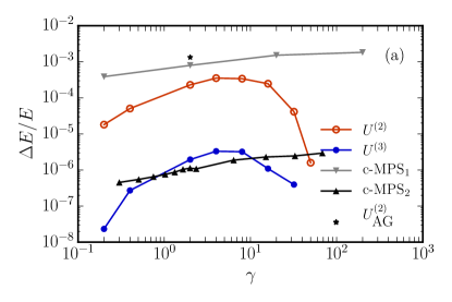
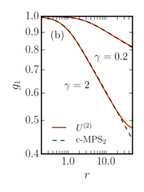
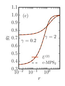
Figure 1: Ground-state properties of the Lieb-Liniger model as obtained from different variational approaches : (a) relative accuracy of the ground-state energy , (b) one-body density matrix, (c) density-density pair correlation functions. $U^{(2)}$ and $U^{(3)}$ denote results for the 2, and 3-body expansion (present work), $U_{\textrm{AG}}^{(2)}$ is the parametrized 2-body Jastrow state of Ref. Astrakharchik and Giorgini (2003), c-MPS₁ results are from Ref. Verstraete and Cirac (2010), and c-MPS₂ are those very recently reported in Ganahl et al. (2016). Distances $r$ are in units of the inverse density $1/n$. Our variational results have been obtained for $N=100$ particles. Finite-size corrections on local quantities are negligible, and very mildly affect the reported large-distances correlations. Overall statistical errors are of the order of symbol sizes, for (a), and line widths, for (b) and (c).

III Lieb-Liniger model

As a first application of the continuous-space t-VMC approach, we consider the Lieb-Liniger model E. H. Lieb and W. Liniger (1963). On one hand, some exact results and numerical data are available, allowing us to benchmark the Jastrow expansion and the t-VMC approach. On the other hand, several aspects of the out-of-equilibrium dynamics of this model are unknown, which we compute here for the first time using t-VMC.

The Lieb-Liniger model describes $N$ interacting bosons in one dimension with contact interactions. It corresponds to the Hamiltonian (1) with $v_{1}(x)=0$ and $v_{2}(x,y)=g\delta(x-y)$, where $g$ is the coupling constant. Here, we consider periodic boundary conditions over a ring of length $L$, and the particle density $n=N/L$. The density dependence is as usual expressed in terms of the dimensionless parameter $\gamma=mg/\hbar^{2}n$. The Lieb-Liniger model is the prototypal model of continuous one-dimensional strongly-correlated gas exactly solvable by Bethe ansatz E. H. Lieb and W. Liniger (1963). This model is experimentally realized in ultracold atomic gases strongly confined in one-dimensional optical traps, and several studies on out-of-equilibrium physics have been already realized Moritz et al. (2003); Kinoshita et al. (2006); Gring et al. (2012); Ronzheimer et al. (2013); Fang et al. (2014); Boéris et al. (2016).

As a result of translation invariance, we have $u_{1}(x\>;t)=\text{const}$, and the first non-trivial term in the many-body expansion (2) is the two-body, translation invariant, function $u_{2}(\left|x-y\right|;t)$. To compute the functional derivatives of the many-body wave function, we proceed with a projection of the continuous Jastrow fields $u_{m}(\mathbf{r};t)$ onto a finite basis set. Here, we have found convenient to represent both the field Hamiltonian (1) and the Jastrow functions, onto a uniform mesh of spacing $a$, leading to $n_{\text{var}}=\frac{L}{2a}$ variational parameters for the $2$-body Jastrow term. In the following our results are extrapolated to the continuous limit, corresponding to $a\rightarrow 0$. The finite-basis projection as well as the numerical time-integration of Eq. (6) are detailed in the Appendix C and benchmarked against exact diagonalization results in the three particle case in Appendix E.

III.1 Ground-state properties

To assess the quality of truncated Bijl-Dingle-Jastrow-Feenberg expansions for the Lieb-Liniger model, we start our analysis considering ground-state properties. An exact solution can be found from the Bethe ansatz (BA) and gives access to exact ground state energies and local properties E. H. Lieb and W. Liniger (1963). Other non-local properties are substantially more difficult to extract from the BA solution, and unbiased results for ground state correlation functions have not been reported so far. In order to determine the best possible variational description of the ground-state within our many-body expansion, different strategies are possible. A first possibility is to consider the imaginary-time evolution $\left|\Psi(\tau)\right\rangle=e^{-\tau\mathcal{H}}\left|\Psi_{0}\right\rangle$ which systematically converges to the exact ground-state in the limit $\tau\gg\Delta_{1}$, where $\Delta_{1}=E_{1}-E_{0}$ is the gap with the first excited state on a finite system and provided that the trial state $\Psi_{0}$ is non-orthogonal to the exact ground state. Imaginary-time evolution in the variational subspace can be implemented considering the formal substitution $t\rightarrow-i\tau$ in the t-VMC equations (6). The resulting equations are equivalent to the stochastic reconfiguration approach Sorella (2001). However, direct minimization of the variational energy can be significantly more efficient, in particular for systems becoming gapless in the thermodynamic limit, where $\Delta_{1}\sim\textrm{poly(}1/N)$. Given the gapless nature of the Lieb-Liniger model, we have found computationally more efficient to adopt a Newton method to minimize the energy variance Umrigar and Filippi (2005).

For the ground state, the many-body expansion truncated at $M=2$ is exact not only in the non-interacting limit $\gamma=0$ but also in the Tonks-Girardeau limit $\gamma\rightarrow\infty$. In this fermionized limit the wave-function can be written as the modulus of a Vandermonde determinant of plane waves, corresponding to the two-body Jastrow function $u_{2}(r)=\log\left(\sin r\pi/L\right)$ Girardeau (1960). To assess the overall quality of pair wave functions for ground state properties, we start comparing the variational ground-state energies $E$ obtained for $M=2$ with the exact BA result. In Fig. 1(a) we show the relative error $\Delta E/E$ as a function of in the interaction strength $\gamma$. We find that the relative error is lower than $10^{-4}$ for all values of $\gamma$ and the accuracy of our two-body Jastrow function is superior to previously published variational results based either on c-MPS Verstraete and Cirac (2010) or VMC Astrakharchik and Giorgini (2003) [see Fig. 1(a) for a quantitative comparison]. Notice that the improvement with respect to previous VMC results is due to the larger variational freedom of our $u_{2}(r)$ function, which is not restricted to any specific functional form as done in Ref. Astrakharchik and Giorgini (2003).

Even though the accuracy reached by the two-body Jastrow function may already be sufficient for most practical purposes for all values of $\gamma$, we have also considered higher order terms with $M=3$, shown in Fig. 2(a). The introduction of the third-order term yields a sizable improvement such that the maximum error is about three orders of magnitude smaller than original c-MPS results Verstraete and Cirac (2010), and feature a similar accuracy of recently reported c-MPS results Ganahl et al. (2016). Overall, our approach reaches a precision on a continuous-space system, which is comparable to state-of-the-art MPS/DMRG results for gapless systems on a lattice Pippan et al. (2010).

Finally, to further assess the quality of our ground state ansatz beyond the total energy, we have also studied non-local properties of the ground state wave function, which are not accessible by existing exact BA methods. In Figs. 1(b) and (c) we show, respectively, our results for the off-diagonal part of the one-body density matrix, $g_{1}(r)\propto\langle\Psi^{\dagger}(r)\Psi(0)\rangle$, and for the pair correlation function, $g_{2}(r)\propto\langle\Psi^{\dagger}(r)\Psi(r)\Psi^{\dagger}(0)\Psi(0)\rangle$, where $\Psi(r)$ is the bosonic field operator. We find an overall excellent agreement with the results that have been obtained with c-MPS in Ref. Ganahl et al. (2016), except for some small deviations at large values of $r$ which we attribute to residual finite-size-effects in our approach. We found that the addition of the 3-body terms does not change significantly correlation functions. Already at the 2-body level, the present results are statistically indistinguishable from exact results obtained using our implementation Carleo et al. (2013) of the worm algorithm Boninsegni et al. (2006) and for the same system (not shown).

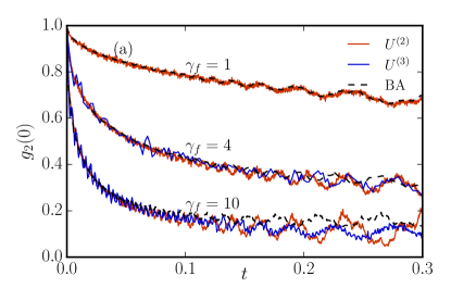
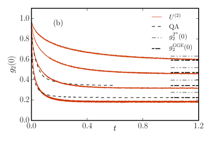
Figure 2: Time-dependent expectation value of local two-body correlations after a quantum quench from a non-interacting state, $\gamma_{i}=0$, to $\gamma_{f}$ : (a) t-VMC results are compared with BA results obtained for a small number of particles Zill et al. (2015, 2016). The correlation function is rescaled to have $g_{2}(0,0)=1$; (b) t-VMC results for $N=100$ particles and $\gamma_{f}=1,2,4,8$ (from top to bottom) compared to the quench action predictions from Ref. De Nardis et al. (2015) (dashed lines), to the Boltzmann thermal averages at the effective temperature $T^{\star}$ (dotted-dashed lines), and to the GGE thermal averages prediction (rightmost dashed lines). Statistical error bars on t-VMC data are of the order of lines width.

III.2 Quench dynamics

Having assessed the quality of the ansatz for local and non-local ground-state properties, we now turn to the study of the out-of-equilibrium properties of the Lieb-Liniger model. We focus on the description of the unitary dynamics induced by a global quantum quench of the interaction strength, from an initial value $\gamma_{i}$ to a final value $\gamma_{f}$. Exact BA results are available only in the case of a non-interacting initial state ($\gamma_{i}=0$). Even in this case, the dynamical BA equations can be exactly solved only for a modest number of particles with further truncation in the number of energy eigen-modes Zill et al. (2015); De Nardis et al. (2015), $N\lesssim 10$, since the complexity of the BA solution increases exponentially with the number of particles. Simplifications in the thermodynamic limit are exploited by the quench action Caux and Essler (2013b), and have been recently applied to quantum quenches starting from a non-interacting initial state De Nardis et al. (2015). In the following we first compare our t-VMC results to these existing results, and then present new results for quenches following a non-vanishing initial interaction strength.

To assess the quality of the time-dependent wave function we compare our results for the evolution of local density-density correlations, $g_{2}(0,t)$, with the truncated BA results obtained in Refs. Zill et al. (2015, 2016) for a small number of particles, $N\simeq 6$. Appendix E provides also further validation of our method accessing $g_{2}(r,t)$ at non-vanishing distances. The comparison shown in Fig. 2(a) shows an overall good agreement. The t-VMC and BA results are indistinguishable for weak interactions ($\gamma_{f}=1$). For larger interactions, we notice systematic but small differences between BA and t-VMC with $M=2$ or $M=3$. These differences amount to a small increase in the amplitude of the oscillations. This effect tends to increase with the interaction strength, being hardly visible for $\gamma=1$ and more pronounced for $\gamma=10$. However, these oscillations result at large times from the discrete mode structure due to the very small number of particles. They vanish in the physical thermodynamic limit. In turn, the comparison at small particle numbers indicates an accuracy better than a few percent for time-averaged quantities in the asymptotic large time limit up to $\gamma=10$, with results at $M=3$ systematically improving on the $M=2$ case. Concerning small and intermediate time scales, we do not observe systematic deviations between the t-VMC results and the BA solution. In particular, the relaxation times are remarkably well captured by the t-VMC approach. On the basis of this comparison and of the comparison for three particles with exact diagonalization results presented in Appendix E, we conclude that t-VMC allows accurate quantitative studies of both the relaxation and equilibration dynamics. This careful benchmarking now allows us to confidently apply the t-VMC approach regimes that are inaccessible to exact BA namely large but finite $N$ and long times, as well as the case of non-vanishing initial interactions.

Let us consider relaxation of density correlations for a large number of particles, close to the thermodynamic limit (here we use $N=100$). As shown in Fig. 2(b), we notice that the amplitudes of the large-time oscillations, attributed to the discrete mode spectrum, are now drastically suppressed compared to the quenches with $N=6$. After an initial relaxation phase, the quantity $g_{2}(0,t)$ approaches a stationary value. Comparing our curves with those obtained with the quench action method, we find a qualitatively good agreement, albeit a general tendency to underestimate the quench action predictions is observed.

We now turn to quenches from interacting initial states ($\gamma_{i}\neq 0$) to different interacting final states for which no results have been obtained by means of exact BA nor simplified quench action method so far. In Fig. 3 we show the asymptotic equilibrium values obtained with our t-VMC approach for quantum quenches from $\gamma_{i}=1$ (Left panel), and $\gamma_{i}=4$ (Right panel) to several values of $\gamma_{f}$. Since, by the variational theorem, the ground state of $\mathcal{H}_{i}$ gives an upper bound for the ground state energy of $\mathcal{H}_{f}$, the system is pushed into a linear combination of excited states of the final hamiltonian. For systems able to thermalize to the Boltzmann ensemble (BE), relaxation to a stationary state described by the density matrix $\rho_{T^{\star}}=e^{-\mathcal{H}_{f}/T^{\star}}$, at an effective temperature $T^{\star}$, would occur. Comparing the stationary value, $\bar{g_{2}}(0)$, of our t-VMC calculations at long times to the thermal values of the pair correlation functions, $g_{2}^{T^{\star}}(0)$, a necessary condition for simple Boltzmann thermalization is given by $\bar{g_{2}}=g_{2}^{T^{\star}}$. The effective temperature, $T^{\star}$, is determined by imposing the energy expectation value of the final Hamiltonian, $\mathcal{H}_{f}$, in the ground state, $\Phi_{0}(\gamma_{i})$ of the initial Hamiltonian, $\langle\mathcal{H}_{\textrm{f}}\rangle_{T^{\star}}=\left\langle\Phi{}_{0}(\gamma_{i})\right|\mathcal{H}_{\text{f}}\left|\Phi{}_{0}(\gamma_{i})\right\rangle$. Here, the thermal expectation value, $\langle\mathcal{H}_{\textrm{f}}\rangle_{T^{\star}}$ at the equilibrium temperature $T^{\star}$ is computed from the Yang-Yang BA equations Yang and Yang (1969). The quantity $\langle\mathcal{H}_{\textrm{f}}\rangle_{T^{\star}}$ then depends on a single parameter $T^{\star}$, that is fitted to match the value of $\left\langle\Phi{}_{0}(\gamma_{i})\right|\mathcal{H}_{\text{f}}\left|\Phi{}_{0}(\gamma_{i})\right\rangle$.

As shown in Fig.2-(b), Boltzmann thermalization certainly does not occur in the case for the Lieb-Liniger model when quenching from a non-interacting state, $\gamma_{i}=0$, where we find $\bar{g_{2}}\neq g_{2}^{T^{\star}}$. This can be understood in terms of the existence of dynamically conserved charges (beyond energy and density conservation) which can yield an equilibrium value substantially different from the BE prediction. In particular, it is widely believe that the Generalized Gibbs Ensemble (GGE) is the correct thermal distribution approached after the quench Rigol (2016); Kollar and Eckstein (2008). Several constructive approaches for the GGE have been put forward in past years Caux and Essler (2013a); Caux and Konik (2012); De Nardis et al. (2015), and the quench action predictions reported in Fig.2-(b) converge to the GGE predictions for the thermal values. In Fig.2-(b) we also show the thermal GGE values $g_{2}^{\text{GGE}}$ (rightmost dashed lines), and notice that our results are much closer to the GGE predictions than the simple BE. Deviations from the asymptotic GGE results are observed at large $\gamma_{f}$, a regime in which the accuracy of our approach is still sufficient to resolve the difference between the BE and the long-term equilibration value.

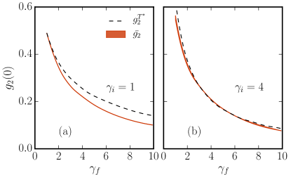
Figure 3: Time-dependent expectation value of local two-body correlations after a quantum quench from the interacting ground state at $\gamma_{i}=1$ (a), and $\gamma_{i}=4$ (b), long-term dynamical averages (red continuous lines) are compared to thermal averages at the effective temperature set by energy conservation (black dashed lines). Uncertainties on the thermal averages of the order of lines width, and are larger for small values of $\gamma_{f}$.

For correlated initial ground states, $\gamma_{i}\neq 0$, GGE predictions are fundamentally harder to obtain than for the non-interacting initial states, and the BE is the only reference thermal distribution we can compare with at this stage. From our results we observe that the difference between $\bar{g_{2}}$ and the simple BE prediction, $g_{2}^{T^{\star}}$, is quantitatively reduced, see Fig. 3. In particular, for $\gamma_{i}=4$, the stationary values $\bar{g_{2}}$ are quantitatively close to the ones predicted by the Boltzmann thermal distribution at the effective temperature $T^{\star}$. Even though this quantitative agreement is likely to be coincidental, the regimes of parameters quenches studied here provide guidance for future experimental studies. In particular, it will be of great interest to understand whether a cross-over from a strongly non-Boltzmann to a close-to-Boltzmann thermal behavior might occur as a function of the initial interaction strength also for other local observables.

IV Conclusions

In this paper we have introduced a novel approach to the dynamics of strongly-correlated quantum systems in continuous space. Our method is based on correlated many-body wave-function systematically expanded in terms of reduced $m$-body Jastrow functions. The unitary dynamics in the subspace of these correlated states was realized using time-dependent variational Monte Carlo. We have demonstrated the possibility or performing calculations up to the three-body level, $m\leq 3$, for the Lieb-Liniger model, for both static and dynamical properties. The improvement from $m=2$ to $m=3$ provides an internal criterium to judge the validity of our results whenever exact results are unavailable. Benchmarking t-VMC with exact or numerical approaches whenever available, we have found a very good agreement with existing results. For static properties, our approach is at the level of state-of-the-art MPS techniques in lattice systems and of latest c-MPS results for interacting gases. For dynamical properties, we have investigated for the first time general interaction quenches which are at the moment unaccessible to Bethe-ansatz approaches. Since the general structure of our t-VMC method does not depend on the dimensionality of the system, it can be directly applied to bosonic systems in higher dimensions with a polynomial increase in computational cost. The methods presented here therefore pave the way to accurate out-of-equilibrium dynamics of two- and three-dimensional quantum gases and fluids beyond mean field approximations.

Appendix A Functional Structure of Many-Body Terms

The local residuals $R^{(M)}(\mathbf{X};t)=i\partial_{t}U^{(M)}(\mathbf{X};t)-E_{\text{loc}}^{(M)}(\mathbf{X};t)$ are vanishing if the Schrödinger equation is exactly satisfied by the many-body wave-function truncated at some order $M$. The local energy $E_{\text{loc}}^{(M)}(\mathbf{X},t)$, however, may contain effective interaction terms involving a number of bodies larger than $M$, which leads to a systematic error in the truncation. However, the structure of these additional terms stemming from the local energy can be systematically used to deduce the functional structure of the higher order terms. For example, the one-body truncated local energy reads, for one-dimensional particles,

$$E_{\text{loc}}^{(1)}(\mathbf{X};t) = -\frac{1}{2}\sum_{i}\left\{\left[\partial_{x_{i}}u_{1}(x_{i};t)\right]^{2}+\partial_{x_{i}}^{2}u_{1}(x_{i};t)\right\}+$$ (7)

$$+\sum_{i}v_{1}(x_{i})+\frac{1}{2}\sum_{i\neq j}^{N}v_{2}(x_{i},x_{j}),$$

and contains a $2$-body term which cannot be accounted for exactly by $u_{1}$. Introduction of a symmetric two-body Jastrow factor $u_{2}(x_{i},x_{j};t)$, then leads to

$$E_{\text{loc}}^{(2)}(\mathbf{X};t) = E_{\text{loc}}^{(1)}(\mathbf{X};t)+$$ (8)

$$-\frac{1}{2}\sum_{i\neq j}\left[\partial_{x_{i}}u_{1}(x_{i};t)\partial_{x_{i}}u_{2}(x_{i},x_{j};t)\right]+$$

$$-\frac{1}{2}\sum_{i\neq j}\partial_{x_{i}}^{2}u_{2}(x_{i},x_{j};t)+$$

$$-\frac{1}{2}\sum_{i\neq j}\sum_{k\neq i}\partial_{x_{i}}u_{2}(x_{i},x_{j};t)\partial_{x_{i}}u_{2}(x_{i},x_{k};t).$$

In the latter expression, one recognizes an effective two-body term which can be accounted for by $u_{2}$ and an additional three-body term in the form of product of two-body functions. The functional form of the three-body Jastrow can be therefore deduced from this additional term and formed accordingly:

$$u_{3}(x_{i},x_{j},x_{k};t) = \bar{u}_{3}(x_{i},x_{j};t)\bar{u}_{3}(x_{j},x_{k};t),$$ (9)

with two-body functions $\bar{u}_{3}(x_{i},x_{j};t)$ containing new variational parameters to be determined. Upon pursuing this approach, the expansion can be systematically pushed to higher orders and the functional structure of the higher order functions inferred. The same constructive approach we have discussed here is also valid for the Schrödinger equation in imaginary-time $\partial_{\tau}U(\mathbf{X};\tau)=-E_{\text{loc}}(\mathbf{x};\tau)$, and has been successfully used to infer the functional structure for ground-state properties Holzmann et al. (2003).

Appendix B Monte Carlo Sampling

In order to solve the t-VMC equations of motion, Eq. (6), expectation values of some given operator $\mathcal{O}$ need to be computed over the many-body wave-function $\Phi(\mathbf{X},t)$. This is achieved by means of Monte Carlo sampling of the probability distribution $\Pi(\mathbf{X})=|\Phi(\mathbf{X})|^{2}$ (In the following we omit explicit reference to the time $t$, assuming that all expectation values are taken over the wave-function at a given fixed time). An efficient way of sampling the given probability distribution is to devise a Markov chain of configurations $\mathbf{X}(1),\mathbf{X}(2),\dots\mathbf{X}(N_{c}-1),\mathbf{X}(N_{c})$ which are distributed according to $\Pi(\mathbf{X})$. Quantum expectation values of a given operator $\mathcal{O}$ can then be obtained as statistical expectation values over the Markov chain as

$$\frac{\left\langle\Phi\right|\mathcal{O}\left|\Phi\right\rangle}{\left\langle\Phi\right|\left.\Phi\right\rangle} \simeq \frac{1}{N_{c}}\sum_{i=1}^{N_{c}}\mathcal{O}_{\text{loc}}(\mathbf{X}(i)),$$ (10)

where $\mathcal{O}_{\text{loc}}(\mathbf{X})=\frac{\left\langle\mathbf{X}\right|\mathcal{O}\left|\Phi\right\rangle}{\left\langle\mathbf{X}\right|\left.\Phi\right\rangle}$, and the equivalence is achieved in the limit $N_{c}\rightarrow\infty$.

The Markov chain is realized by the Metropolis-Hastings algorithm. Given the current state of the Markov chain, $\mathbf{X}(i)$, a configuration $\mathbf{X^{\prime}}$ is generated according to a given transition probability $T(\mathbf{X}(i)\rightarrow\mathbf{X}^{\prime})$. The proposed configuration is then accepted (i.e. $\mathbf{X}(i+1)=\mathbf{X}^{\prime}$ ) with probability

$$A(\mathbf{X}(i)\rightarrow\mathbf{X}^{\prime})=\\ =\text{min}\left[1,\frac{\Pi(\mathbf{X}^{\prime})}{\Pi(\mathbf{X}(i))}\frac{T(\mathbf{X}^{\prime}\rightarrow\mathbf{X}(i))}{T(\mathbf{X}(i)\rightarrow\mathbf{X}^{\prime})}\right],$$ (11)

otherwise it is rejected and $\mathbf{X}(i+1)=\mathbf{X}(i)$.

In the present t-VMC calculations we use simple transition probabilities in which a single particle is displaced, while leaving all the other particles positions unchanged. In particular, a particle index $p$ is chosen with uniform probability $1/N$ and the position of particle $p$ is then displaced according to $x_{p}^{\prime}=x_{p}+\eta_{\Delta}$, where $\eta_{\Delta}$ is a random number uniformly distributed in $[-\frac{\Delta}{2},\frac{\Delta}{2}]$. The amplitude $\Delta$ is an adjustable parameter and it can be typically chosen to be of the order of the average inter-particle distance. With this choice, the transition probability is simply

$$T(x_{p}\rightarrow x_{p}^{\prime}) = \frac{1}{N\Delta},$$ (12)

and the acceptance probability is therefore given by the mere ratio of the probability distributions, $\frac{\Pi(\mathbf{X}^{\prime})}{\Pi(\mathbf{X}(i))}$.

Appendix C Finite Basis Projection

The numerical solution of the equations of motion (6) requires the projection of the Jastrow fields $u_{m}(\mathbf{r};t)$ onto a finite basis. The continuous variable $\mathbf{r}$ is reduced to a finite set of $P$ values for each order $m$, $(m,\mathbf{r})\rightarrow(r_{1,m},r_{2,m}\dots r_{P,m})$. We introduced a super-index $K$ spanning all possible values of the discrete variables $r_{i,m}$. The complete set of variational parameters resulting from the projection on the finite basis can then be written as $u_{K}(t)$ and the associated functional derivatives read $\rho_{K}(t)$.

The integro-differential equations (6) are then brought to the algebraic form

$$\sum_{K^{\prime}}S_{K,K^{\prime}}\dot{u}_{K^{\prime}}(t) = -i\left\langle E_{\text{loc}}(t)\rho_{K}(t)\right\rangle,$$ (13)

where we have introduced the Hermitian correlation matrix

$$S_{K,K^{\prime}}(t) = \frac{\partial\left\langle\rho_{K}(t)\right\rangle_{t}}{\partial u_{K^{\prime}}}=$$ (14)

$$= \left\langle\rho_{K}(t)\rho_{K^{\prime}}(t)\right\rangle_{t}-\left\langle\rho_{K}(t)\right\rangle_{t}\left\langle\rho_{K^{\prime}}(t)\right\rangle_{t}.$$

At a given time, all the expectations values in Eq. (13) can be explicitly computed with the stochastic approach described in Appendix B. We are therefore left with a linear system in the $n_{\text{var}}$ unknowns $\dot{u}_{K}(t)$, which needs to be solved at each time $t$.

In the presence of a large number of variational parameters, $n_{\text{var}}$, the solution of the linear system can be achieved using iterative solvers e.g., conjugate gradient methods, which do not need to explicitly form the matrix $S$. Calling $n_{\text{iter}}$ the number of iterations needed to obtain a solution for the linear system, the computational cost to solve (13) is $\mathcal{O}(M\times n_{\text{var}}\times n_{\text{iter}})$ as opposed to the $\mathcal{O}(M\times n_{\text{var}}^{2})$ operations needed by a standard solver in which the matrix $S$ is formed explicitly. In the present work we resort to the Minimal Residual (MinRes) method, which is a variant of the Lanczos method, working in the Krylov subspace spanned by the repeated action of the matrix $S$ onto an initial vector. In typical applications we obtain that $n_{\text{iter}}\ll n_{\text{var}}$ and several thousands of variational parameters can be efficiently treated. This is of fundamental importance when the continuous (infinite-basis) limit must be taken, for which $n_{\text{var}}\rightarrow\infty$.

Once the unknowns $\dot{u}_{K}(t)$ are determined, we can solve numerically the first-order differential equations given in Eq. (6) for given initial conditions $u_{K}(0)$. In the present work we have adopted an adaptive 4th order Runge-Kutta scheme for the integration of the differential equations.

Appendix D Lattice Regularization For The Lieb-Liniger Model

We consider a general wave-function $\Psi(x_{1},x_{2}\dots x_{N})$ for $N$ one-dimensional particles, governed by the Lieb-Liniger Hamiltonian. By means of Variational Monte Carlo, we want to sample $|\Phi(\mathbf{X})|^{2}$, this is achieved via a lattice regularization, i.e.

$$\int d\mathbf{X}|\Phi(\mathbf{X})|^{2} \simeq \sum_{l_{1},l_{2}\dots l_{N}}|\Phi(l_{1},l_{2}\dots l_{N})|^{2}$$

where $l_{i}=\{0,a,\dots L-a\}$ are discrete particle positions, $a$ the lattice spacing, $L$ the box size and $N_{s}=1+L/a$ the number of lattice sites. As a discretized Hamiltonian we take

$$H_{a}\Phi(l_{1}\dots l_{N})=-\frac{\hbar^{2}}{2ma^{2}}\sum_{i}\left\{\frac{4}{3}\left[\Phi(l_{1}\dots l_{i}-a,\dots l_{N})\right.+\right.\\ \left.\Phi(l_{1}\dots l_{i}+a,\dots l_{N})\right]-\\ \frac{1}{12}\left[\Phi(l_{1}\dots l_{i}-2a,\dots l_{N})+\Phi(l_{1}\dots l_{i}+2a,\dots l_{N})\right]+\\ \left.-\frac{5}{2}\Phi(l_{1}\dots l_{i},\dots l_{N})\right\}+\Phi(l_{1}\dots l_{N})\frac{g}{a}\sum_{i<j}\delta(l_{i},l_{j})$$

The first terms constitute just the fourth-order approximation of the laplacian via central finite differences, whereas the last term corresponds the two-body delta interaction part.

With this discretization, a two-body Jastrow factor reads

$$u_{2}(x_{ij};t) = u_{2}(l_{i},l_{j};t),$$

where $u_{2}(a,b;t)$ is a time-dependent matrix of size $N_{s}\times N_{s}$ which, in 1D and in the presence of translational symmetry, depends only on $\textrm{dist}(a-b)$, i.e. it has $N_{s}/2$ variational parameters.

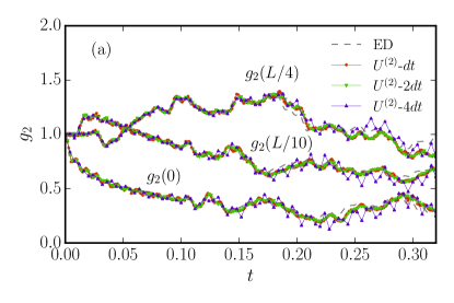
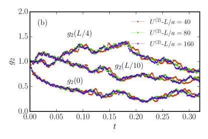
Figure 4: Time-dependent expectation value of the two-body correlations after a quantum quench from a non-interacting state, $\gamma_{i}=0$, to $\gamma_{f}=4$ at three different distance $|x_{1}-x_{2}|=0,L/10,L/4$. Here, the system is on a lattice with $L/a=40$ lattice sites, the full line is obtained by exact diagonalization of the Hamiltonian, the other curves are from tVMC truncated at the level of $U^{(2)}$. In the left figure (a), we show the convergence with different time step discretization. On the right figure (b), we show the approach to the continuum for t-VMC simulations using $U^{(2)}$ for discretizations $L/a=40$, $80$ and $160$.

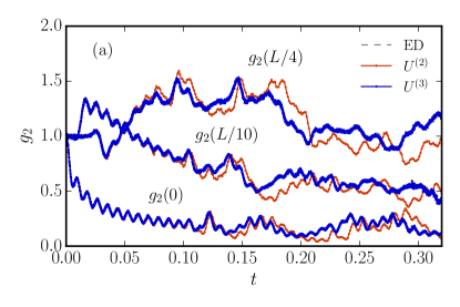
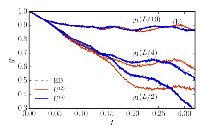
Figure 5: (a) Time-dependent expectation value of the two-body correlations, $g_{2}(r,t)$, after a quantum quench from a non-interacting state, $\gamma_{i}=0$, to $\gamma_{f}=8$ at three different distance $|x_{1}-x_{2}|=0,L/10,L/4$. Here, the system is on a lattice with $L/a=40$ lattice sites, the full line is obtained by exact diagonalization of the Hamiltonian, the other curves are from t-VMC truncated at the level of $U^{(2)}$ or $U^{(3)}$. In contrast to $\gamma_{f}=4$ shown in Fig.4, systematic differences of $U^{(2)}$ compared to the exact results are more visible here, the exact dynamics is recovered by inclusion of three-body terms, $U^{(3)}$, into the tVMC wave function. (b) shows the off-diagonal single particle density matrix, $g_{1}(r,t)$, at three different distances, $r=L/10$, $L/4$ and $L/2$.

Appendix E Benchmark Study for $N=3$ on a Lattice

Here, we use exact diagonalization of a Hamiltonian within a given finite basis for a quantitative test of our method. Exact diagonalization is limited to very small systems on a finite basis, and we haven chosen a system containing $N=3$ particles on $L/a=40$ lattice sites as a simple, but highly non-trivial reference. In contrast to our comparison with BA methods, all observables can be accessed by exact diagonalization and we have used the off-diagonal one body density matrix $g_{1}(r,t)$ and the pair correlation function $g_{2}(r,t)$ at different distances $r=|x_{1}-x_{2}|$ of two particles after time $t$ where the system is quenched from the non-interacting initial state, $\gamma_{i}=0$, to a final interaction $\gamma_{f}>0$, to provide a benchmark on a more general observable.

We first benchmark the influence of the time-step lattice size discretization $\Delta t$ error on $g_{2}$. From Fig.4(a) we see that the t-VMC dynamics is stable over a long time and the time step error can be brought to convergence. Further, we see that for final interaction $\gamma_{f}=4$ the truncation at the two-body level, $U^{(2)}$, introduces only a small systematic error, mainly a dephasing effect, which is almost negligible at the scale of the figure. Due to the stochastic noise of the Monte Carlo integration, t-VMC introduces additional high frequency oscillations which are, however, well separable from the deterministic propagation. The amplitude of these high frequency oscillations also quantifies the purely statistical error of our data.

Whereas exact diagonalization is limited to rather small basis sets, we can access much a larger basis within t-VMC. In Fig.4 (b) we show results within the $U^{(2)}$ approximation with $L/a=80$ and $L/a=160$ with time discretization $\Delta t\sim(L/a)^{2}$. We see that the basis set truncation in general introduces a dephasing at large enough time.

The systematic error of $U^{(2)}$ increases towards quenches to stronger interaction strength and becomes more visible for $\gamma_{f}=8$ shown in Fig.5(a). However, even in this case, the most important effect remains to be a simple dephasing, a small shift of averaged quantities is probable, but difficult to quantify precisely. Introducing a general three-body Jastrow fields, $U^{(3)}$, described in detail in Appendix F, the systematic error for $N=3$ can be fully eliminated.

In figure 5 (b), we also benchmark the possibility of calculating the off-diagonal one-body density matrix after a quench. Here the systematic error of $U^{(2)}$ is more pronounced at smaller $\gamma_{f}$ in the long range and time regime.

From our study of the three particle problem, we conclude that truncation of the many-body wave function at the level of $U_{2}$ may provide an excellent approximation for $g_{2}(r,t)$ for quenches involving not too strong interaction strengths, $\gamma\lesssim 5$. The systematic error due to the $U^{(2)}$ truncation is mainly a dephasing at large times involving small relative errors of time averaged quantities. Similar systematic dephasing errors will occur for too large time discretization or basis set truncation.

Since our method provides a parametrization of the full wave function for a given time, many different observables can be evaluated via usual Monte Carlo methods. However, the quality of different observables may vary and depend more sensitive on the inclusion of higher order correlations $U^{(n)}$ with $n>2$ as in the case of the single body density matrix. Although these higher order terms are computationally expensive, the scaling is not exponential, and we have explicitly shown that calculations with $n=3$ are feasible. We notice that the computational complexity may be further reduced by functional forms adapted to the problem (Holzmann et al., 2006).

Appendix F General Structure of $U^{(3)}$

For a general time dependent wave function, we have to go beyond the usual ground state structure of the three-body Jastrow given in Eq. (9). Here, we provide details of our three-body term in a general form beyond the present application in one dimension.

Introducing $M$ basis functions, $b^{a}(r)$, $a=1,\dots M$, we can introduce many-body vectors (Holzmann et al., 2006), $B_{i\alpha}^{a}=\sum_{j}{\bf r}_{ij}^{\alpha}b^{a}(r_{ij})$, where $\alpha=1,\dots D$ indicates the summation over directions and $i=1,\dots N$. The variational parameters of a general three-body structure can then be written in terms of a matrix $w_{ab}$, such that

$$\sum_{i\neq j\neq k}u_{3}({\bf r}_{1},{\bf r}_{2},{\bf r}_{3})=\sum_{ab}w_{ab}W^{ab},\quad W^{ab}=\sum_{i\alpha}B_{i\alpha}^{a}B_{i\alpha}^{b}$$ (15)

In order to reduce the variational parameters ($\sim M^{2}$), we may perform a singular value decomposition of the matrix $w_{ab}$ to reduce the effective degrees of freedom.