Numerical approximation of BSDEs using local polynomial drivers and branching processes

Abstract

We propose a new numerical scheme for Backward Stochastic Differential Equations based on branching processes. We approximate an arbitrary (Lipschitz) driver by local polynomials and then use a Picard iteration scheme. Each step of the Picard iteration can be solved by using a representation in terms of branching diffusion systems, thus avoiding the need for a fine time discretization. In contrast to the previous literature on the numerical resolution of BSDEs based on branching processes, we prove the convergence of our numerical scheme without limitation on the time horizon. Numerical simulations are provided to illustrate the performance of the algorithm.

Keywords: Bsde, Monte-Carlo methods, branching process.

MSC2010: Primary 65C05, 60J60; Secondary 60J85, 60H35.

1 Introduction

Since the seminal paper of Pardoux and Peng [22], the theory of Backward Stochastic Differential Equations (BSDEs hereafter) has been largely developed, and has lead to many applications in optimal control, finance, etc. (see e.g. El Karoui, Peng and Quenez [11]). Different approaches have been proposed during the last decade to solve them numerically, without relying on pure PDE based resolution methods. A first family of numerical schemes, based on a time discretization technique, has been introduced by Bally and Pagès [2], Bouchard and Touzi [5] and Zhang [30], and generated a large stream of the literature. The implementation of these numerical schemes requires the estimation of a sequence of conditional expectations, which can be done by using simulations combined with either non-linear regression techniques or Malliavin integration by parts based representations of conditional expectations, or by using a quantization approach, see e.g. [6, 15] for references and error analysis.

Another type of numerical algorithms is based on a pure forward simulation of branching processes, and was introduced by Henry-Labordère [17], and Henry-Labordère, Tan and Touzi [19] (see also the recent extension by Henry-Labordère et al. [18]). The main advantage of this new algorithm is that it avoids the estimation of conditional expectations. It relies on the probabilistic representation in terms of branching processes of the so-called KPP (Kolmogorov-Petrovskii-Piskunov) equation:

$$\partial_{t}u(t,x)~{}+~{}\frac{1}{2}D^{2}u(t,x)~{}+~{}\sum_{k\geq 0}p_{k}u^{k}(t,x)~{}=~{}0,~{}~{}~{}u(T,x)=g(x).$$ (1)

Here, $D^{2}$ is the Laplacian on $\mathbb{R}^{d}$, and $(p_{k})_{k\geq 0}$ is a probability mass sequence, i.e. $p_{k}\geq 0$ and $\sum_{k\geq 0}p_{k}=1$. This is a natural extension of the classical Feynmann-Kac formula, which is well known since the works of Skorokhod [24], Watanabe [29] and McKean [21], among others. The PDE (1) corresponds to a BSDE with a polynomial driver and terminal condition $g(W_{T})$:

$$Y_{\cdot}=g(W_{T})+\int_{\cdot}^{T}\sum_{k\geq 0}p_{k}(Y_{t})^{k}dt-\int_{\cdot}^{T}Z_{t}dW_{t},$$

in which $W$ is a Brownian motion. Since $Y_{\cdot}=u(\cdot,W_{\cdot})$, the $Y$-component of this BSDE can be estimated by making profit of the branching process based Feynman-Kac representation of (1) by means of a pure forward Monte-Carlo scheme, see Section 2.3 below. The idea is not new. It was already proposed in Rasulov, Raimov and Mascagni [23], although no rigorous convergence analysis was provided. Extensions to more general drivers can be found in [17, 18, 19]. Similar algorithms have been studied by Bossy et al. [4] to solve non-linear Poisson-Boltzmann equations.

It would be tempting to use this representation to solve BSDEs with Lipschitz drivers, by approximating their drivers by polynomials. This is however not feasible in general. The reason is that PDEs (or BSDEs) with polynomial drivers, of degree bigger or equal to two, typically explode in finite time. They are only well posed on a small time interval. It is worse when the degree of the polynomial increases. Hence, no convergence can be expected for the case of general drivers.

In this paper, we propose to instead use a local polynomial approximation. Then, convergence of the sequence of approximating drivers to the original one can be ensured without explosion of the corresponding BSDEs, that can be defined on a arbitrary time interval. It requires to be combined with a Picard iteration scheme, as the choice of the polynomial form will depend on the position in space of the solution $Y$ itself. However, unlike classical Picard iteration schemes for BSDEs, see e.g. Bender and Denk [3], we do not need to have a very precise estimation of the whole path of the solution at each Picard iteration. Indeed, if local polynomials are fixed on a partition $(A_{i})_{i}$ of $\mathbb{R}$, then one only needs to know in which $A_{i}$ the solution stays at certain branching times of the underlying branching process. If the $A_{i}$’s are large enough, this does not require a very good precision in the intermediate estimations. We refer to Remark 2.10 for more details.

We finally insist on the fact that our results will be presented in a Markovian context for simplification. However, all of our arguments work trivially in a non-Markovian setting too.

2 Numerical method for a class of BSDE based on branching processes

Let $T>0$, $W$ be a standard $d$-dimensional Brownian motion on a filtered probability space $(\Omega,{\cal F},\mathbb{F}=({\cal F}_{t})_{t\geq 0},\mathbb{P})$, and $X$ be the solution of the stochastic differential equation:

$${X}=X_{0}+\int_{0}^{\cdot}\mu({X}_{s})\,dt+\int_{0}^{\cdot}\sigma({X}_{s})\,dW_{s},$$ (2)

where $X_{0}$ is a constant, lying in a compact subset $\mathbf{X}$ of $\mathbb{R}^{d}$, and $(\mu,\sigma):[0,T]\times\mathbb{R}^{d}\mapsto\mathbb{R}^{d}\times\mathbb{M}^{d}$ is assumed to be Lipschitz continuous with support contained in $\mathbf{X}$. Our aim is to provide a numerical scheme for the resolution of the backward stochastic differential equation

$$Y_{\cdot}=g({X}_{T})+\int_{\cdot}^{T}f({X}_{s},Y_{s})\,ds-\int_{\cdot}^{T}Z_{s}\,dW_{s}.$$ (3)

In the above, $g:\mathbb{R}^{d}\mapsto\mathbb{R}$ is assumed to be measurable and bounded, $f\in\mathbb{R}^{d}\times\mathbb{R}\mapsto\mathbb{R}$ is measurable with linear growth and Lipschitz in its second argument, uniformly in the first one. As a consequence, there exists $M\geq 1$ such that

$$|g(X_{T})|\leq M\;\mbox{ and }|X|+|Y|\leq M\;\mbox{ on }[0,T].$$ (4)

Remark 2.1.

The above conditions are imposed to easily localize the solution $Y$ of the BSDE, which will be used in our estimates later on. One could also assume that $g$ and $f$ have polynomial growth in their first component and that $\mathbf{X}$ is not compact. After possibly truncating the coefficients and reducing their support, one would go back to our conditions. Then, standard estimates and stability results for SDEs and BSDEs could be used to estimate the additional error in a very standard way. See e.g. [11].

2.1 Local polynomial approximation of the generator

A first main ingredient of our algorithm consists in approximating the driver $f$ by a driver $f_{\ell_{\circ}}$ that has a local polynomial structure. Namely, let

$$f_{\ell_{\circ}}:(x,y,y^{\prime})\in\mathbb{R}^{d}\times\mathbb{R}\times\mathbb{R}\mapsto\sum_{j=1}^{j_{\circ}}\sum_{\ell=0}^{\ell_{\circ}}a_{j,\ell}(x)y^{\ell}\varphi_{j}(y^{\prime}),$$ (5)

in which $(a_{j,\ell},\varphi_{j})_{\ell\leq\ell_{\circ},j\leq j_{\circ}}$ is a family of continuous and bounded maps satisfying

$$|a_{j,\ell}|\leq C_{\ell_{\circ}}\;,\;|\varphi_{j}(y^{\prime}_{1})-\varphi_{j}(y^{\prime}_{2})|\leq L_{\varphi}|y^{\prime}_{1}-y^{\prime}_{2}|\mbox{ and }|\varphi_{j}|\leq 1,$$ (6)

for all $y^{\prime}_{1},y^{\prime}_{2}\in\mathbb{R}$, $j\leq j_{\circ}$ and $\ell\leq\ell_{\circ}$, for some constants $C_{\ell_{\circ}},L_{\varphi}\geq 0$. In the following, we shall assume that $\ell_{\circ}\geq 2$ (without loss of generality). One can think of the $(a_{j,\ell})_{\ell\leq\ell_{\circ}}$ as the coefficients of a polynomial approximation of $f$ on a subset $A_{j}$, the $A_{j}$’s forming a partition of $[-M,M]$. Then, the $\varphi_{j}$’s have to be considered as smoothing kernels that allow one to pass in a Lipschitz way from one part of the partition to another one. We therefore assume that

$${\#\{j\in\{1,\cdots,j_{\circ}\}:\;\varphi_{j}(y)>0\}\leq 2\;\mbox{ for all }y\in\mathbb{R},}$$ (7)

and that $y\mapsto f_{\ell_{\circ}}(x,y,y)$ is globally Lipschitz. In particular,

$$\bar{Y}_{\cdot}=g({X}_{T})+\int_{\cdot}^{T}f_{\ell_{\circ}}({X}_{s},\bar{Y}_{s},\bar{Y}_{s})\,ds-\int_{\cdot}^{T}\bar{Z}_{s}\,dW_{s},$$ (8)

has a unique solution $(\bar{Y},\bar{Z})$ such that $\mathbb{E}[\sup_{[0,T]}|\bar{Y}|^{2}]<\infty$. Moreover, by standard estimates, $(\bar{Y},\bar{Z})$ provides a good approximation of $(Y,Z)$ whenever $f_{\ell_{\circ}}$ is a good approximation of $f$:

$$\mathbb{E}\Big{[}\sup_{[0,T]}|Y-\bar{Y}|^{2}\Big{]}+\mathbb{E}\Big{[}\!\!\int_{0}^{T}\!\!\!\!|Z_{t}-\bar{Z}_{t}|^{2}dt\Big{]}\leq C\mathbb{E}\Big{[}\!\!\int_{0}^{T}\!\!\!|f-f_{\ell_{\circ}}|^{2}(X_{t},Y_{t},Y_{t})dt\Big{]},$$ (9)

for some $C>0$ that does not depend on $f_{\ell_{\circ}}$, see e.g. [11].

The choice of $f_{\ell_{\circ}}$ will obviously depend on the application at hand and does not need to be more commented. Let us just mention that our algorithm will be more efficient if the sets $\{y\in\mathbb{R}:\varphi_{j}(y)=1\}$ are large and the intersection between the supports of the $\varphi_{j}$’s are small, see Remark 2.10 below.

We also assume that

$$|\bar{Y}|\leq M.$$ (10)

Since we intend to keep $f_{\ell_{\circ}}$ with linear growth in its first component, and bounded in the two other ones, uniformly in $\ell_{\circ}$, this is without loss of generality.

2.2 Picard iteration with doubly reflected BSDEs

Our next step is to introduce a Picard iteration scheme to approximate the solution $\bar{Y}$ of (8). Note however that, although the map $y\mapsto f(x,y,y)$ is globally Lipschitz, the map $y\mapsto f(x,y,y^{\prime})$ is a polynomial, given $y^{\prime}$, and hence only locally Lipschitz in general. In order to reduce to a Lipschitz driver, we shall apply our Picard scheme to a doubly (discretely) reflected BSDE, with lower and upper barrier given by the bounds $-M$ and $M$ for $\bar{Y}$, recall (10).

Let $h_{\circ}$ be defined by (27) in the Appendix. It is a lower bound for the explosion time of the BSDE with driver $y\mapsto f(x,y,y^{\prime})$. Let us then fix $h\in(0,h_{\circ})$ such that $N_{h}:=T/h\in\mathbb{N}$, and define

$${t_{i}}=ih\;\;\;\;\;\mbox{and}\;\;\;\;\mathbb{T}:=\{{t_{i}},~{}i=0,\cdots,N_{h}\}.$$ (11)

We initialize our Picard scheme by setting

$$\bar{Y}^{0}_{t}={\rm y}(t,X_{t})\;\mbox{ for }t\in[0,T],$$ (12)

in which ${\rm y}$ is a deterministic function, bounded by $M$ and such that ${\rm y}(T,\cdot)=g$. Then, given $\bar{Y}^{m-1}$, for $m\geq 1$, we define $(\bar{Y}^{m},\bar{Z}^{m},\bar{K}^{m,+},\bar{K}^{m,-})$ as the solution on $[0,T]$ of

$$\bar{Y}^{m}_{t}=g(X_{T})+\int_{t}^{T}{f}_{\ell_{\circ}}(X_{s},\bar{Y}^{m}_{s},\bar{Y}^{m-1}_{s})\,ds-\int_{t}^{T}\bar{Z}^{m}_{s}\,dW_{s}+\int_{[t,T]\cap\mathbb{T}}\!\!\!\!\!d(\bar{K}^{m,+}-\bar{K}^{m,-})_{s},\;\;\;$$

$$-M\leq\bar{Y}^{m}_{t}\leq M,~{}~{}~{}\forall t\in\mathbb{T},~{}a.s.$$ (13)

$$\int_{\mathbb{T}}(\bar{Y}^{m}_{s}+M)d\bar{K}^{m,+}_{s}=\int_{\mathbb{T}}(\bar{Y}^{m}_{s}-M)d\bar{K}^{m,-}_{s}=0,$$

where $\bar{K}^{m,+}$ and $\bar{K}^{m,-}$ are non-decreasing processes.

Remark 2.2.

Since the solution $\bar{Y}$ of (8) is bounded by $M$, the quadruple of processes $(\bar{Y},\bar{Z},\bar{K}^{+},\bar{K}^{-})$ (with $\bar{K}^{+}\equiv\bar{K}^{-}\equiv 0$) is in fact the unique solution of the same reflected BSDE as in (13) but with $f_{\ell_{\circ}}(X,\bar{Y},\bar{Y})$ in place of ${f}_{\ell_{\circ}}(X_{s},\bar{Y}^{m},\bar{Y}^{m-1})$.

Remark 2.3.

One can equivalently define the process $\bar{Y}^{m}$ in a recursive way. Let $\bar{Y}^{m}_{T}:=g(X_{T})$ be the terminal condition, and define, on each interval $[t_{i},t_{i+1}]$, $(Y^{m}_{\cdot},Z^{m}_{\cdot})$ as the solution on $[t_{i},t_{i+1}]$ of

$$Y^{m}_{\cdot}~{}=~{}\bar{Y}^{m}_{t_{i+1}}+\int^{t_{i+1}}_{\cdot}\!\!\!\!f_{\ell_{\circ}}(X_{s},Y^{m}_{s},\bar{Y}^{m-1}_{s})ds-\int^{t_{i+1}}_{\cdot}Z^{m}_{s}dW_{s}.\;\;$$ (14)

Then, $\bar{Y}^{m}:=Y^{m}$ on $(t_{i},t_{i+1}]$, and $\bar{Y}^{m}_{t_{i}}:=(-M)\vee Y^{m}_{t_{i}}\wedge M$.

The error due to our Picard iteration scheme is handled in a standard way. It depends on the constants

$$L_{1}:=2C_{\ell_{\circ}}\sum_{\ell=1}^{\ell_{\circ}}\ell(M_{h_{\circ}})^{\ell-1},\;\;\;M_{h_{\circ}}L_{2}:=L_{\varphi}\sum_{\ell=0}^{\ell_{\circ}}2C_{\ell_{\circ}}(M_{h_{\circ}})^{\ell},$$

where $M_{h_{\circ}}$ is defined by (28).

Theorem 2.4.

The system (13) admits a unique solution $(\bar{Y}^{m},\bar{Z}^{m},\bar{K}^{m,+},\bar{K}^{m,-})_{m\geq 0}$ such that $\bar{Y}^{m}$ is uniformly bounded for each $m\geq 0$. Moreover, for all $m\geq 0$, $|\bar{Y}^{m}|$ is uniformly bounded by the constant $M_{h_{\circ}}$, and

$$|\bar{Y}^{m}_{t}-\bar{Y}_{t}|^{2}~{}\leq~{}\frac{L_{2}}{\lambda^{2}}\Big{(}\frac{L_{2}(T-t)}{\lambda^{2}}\Big{)}^{m}(2M)^{2}\frac{e^{\beta T}}{\beta},$$

for all $t\leq T$, and all constants $\lambda>0$, $\beta>2L_{1}+L_{2}\lambda^{2}$.

Proof. $\mathrm{i)}$ First, when $\bar{Y}^{m}$ is uniformly bounded, $f_{\ell_{\circ}}(X_{s},\bar{Y}^{m}_{s},\bar{Y}^{m-1}_{s})$ can be considered to be uniformly Lipschitz in $\bar{Y}^{m}$, then (13) has at most one bounded solution. Next, in view of Lemma A.1 and Remark 2.3, it is easy to see that (14) has a unique solution $Y^{m}$, bounded by $M_{h_{\circ}}$ (defined by (28)) on each interval $[t_{i},t_{i+1}]$. It follows the existence of the solution to (13). Moreover, $\bar{Y}^{m}$ is also bounded by $M_{h_{\circ}}$ on $[0,T]$, and more precisely bounded by $M$ on the discrete grid $\mathbb{T}$, by construction.

$\mathrm{ii)}$ Consequently, the generator $f_{\ell_{\circ}}(x,y,y^{\prime})$ can be considered to be uniformly Lipschitz in $y$ and $y^{\prime}$. Moreover, using (6) and (7), one can identify the corresponding Lipschitz constants as $L_{1}$ and $L_{2}$.

Let us denote $\Delta\bar{Y}^{m}:=\bar{Y}^{m}-\bar{Y}$ for all $m\geq 1$. We notice that, in Remark 2.3, the truncation operation $\bar{Y}^{m}_{t_{i}}:=(-M)\vee Y^{m}_{t_{i}}\wedge M$ can only make the value $(\Delta\bar{Y}^{m}_{{t_{i}}})^{2}$ smaller than $(Y^{m}_{t_{i}}-\bar{Y}_{t_{i}})^{2}$, since $|\bar{Y}|\leq M$. Thus we can apply Itô’s formula to $(e^{\beta t}(\Delta\bar{Y}^{m+1}_{t})^{2})_{t\geq 0}$ on each interval $[t_{i},t_{i+1}]$, and then take expectation to obtain

$$\mathbb{E}\big{[}e^{\beta t}(\Delta\bar{Y}^{m+1}_{t})^{2}\big{]}+\beta\mathbb{E}\Big{[}\int_{t}^{T}e^{\beta s}|\Delta\bar{Y}^{m+1}_{s}|^{2}ds+\int_{t}^{T}e^{\beta s}|\Delta\bar{Z}^{m+1}_{s}|^{2}ds\Big{]}$$

$$\leq 2\mathbb{E}\Big{[}\int_{t}^{T}e^{\beta s}\Delta\bar{Y}^{m+1}_{s}\big{(}f_{\ell_{\circ}}(X_{s},\bar{Y}^{m+1}_{s},\bar{Y}^{m}_{s})-f_{\ell_{\circ}}(X_{s},\bar{Y}_{s},\bar{Y}_{s})\big{)}ds\Big{]}.$$

Using the Lipschitz property of $f_{\ell_{\circ}}$ and the inequality $\lambda^{2}+\frac{1}{\lambda^{2}}\geq 2$, it follows that the r.h.s. of the above inequality is bounded by

$$(2L_{1}+L_{2}\lambda^{2})\mathbb{E}\Big{[}\int_{t}^{T}e^{\beta s}(\Delta\bar{Y}^{m+1}_{s})^{2}ds\Big{]}+\frac{L_{2}}{\lambda^{2}}\mathbb{E}\Big{[}\int_{t}^{T}e^{\beta s}(\Delta\bar{Y}^{m}_{s})^{2}ds\Big{]}.$$

Since $\beta\geq 2L_{1}+L_{2}\lambda^{2}$, the above implies

$$\mathbb{E}\Big{[}e^{\beta t}(\Delta\bar{Y}_{t}^{m+1})^{2}\Big{]}~{}\leq~{}\frac{L_{2}}{\lambda^{2}}\mathbb{E}\Big{[}\int_{t}^{T}e^{\beta s}(\Delta\bar{Y}^{m}_{s})^{2}ds\Big{]},$$ (15)

and hence

$$\mathbb{E}\Big{[}\int_{0}^{T}e^{\beta t}(\Delta\bar{Y}_{t}^{m+1})^{2}dt\Big{]} \leq \frac{L_{2}}{\lambda^{2}}T\mathbb{E}\Big{[}\int_{0}^{T}e^{\beta s}(\Delta\bar{Y}^{m}_{s})^{2}ds\Big{]}.$$

Since $|\Delta\bar{Y}^{0}|=|{\rm y}(\cdot,X)-\bar{Y}|\leq 2M$ by (10) and our assumption $|{\rm y}|\leq M$, this shows that

$$\mathbb{E}\Big{[}\int_{0}^{T}e^{\beta t}(\Delta\bar{Y}_{t}^{m})^{2}dt\Big{]} \leq \big{(}\frac{L_{2}}{\lambda^{2}}T\big{)}^{m}(2M)^{2}e^{\beta T}/\beta.$$

Plugging this in (15) leads to the required result at $t=0$. It is then clear that the above estimation does not depend on the initial condition $(0,X_{0})$, so that the same result holds true for every $t\in[0,T]$. ∎

2.3 A branching diffusion representation for $\bar{Y}^{m}$

We now explain how the solution of (14) on $[t_{i},t_{i+1})$ can be represented by means of a branching diffusion system. More precisely, let us consider an element $(p_{\ell})_{0\leq\ell\leq\ell_{\circ}}\in\mathbb{R}^{\ell_{\circ}+1}_{+}$ such that $\sum_{\ell=0}^{\ell_{\circ}}p_{\ell}=1$, set $K_{n}:=\{(1,k_{2},\ldots,k_{n}):(k_{2},\ldots,k_{n})\in\{0,\ldots,\ell_{\circ}\}^{n}\}$ for $n\geq 1$, and $K:=\cup_{n\geq 1}K_{n}$. Let $(W^{k})_{k\in K}$ be a sequence of independent $d$-dimensional Brownian motions, $(\xi_{k})_{k\in K}$ and $(\delta_{k})_{k\in K}$ be two sequences of independent random variables, such that

$$\mathbb{P}[\xi_{k}=\ell]=p_{\ell},\,\;\ell\leq\ell_{\circ},k\in K,$$

and

$$\bar{F}(t):=\mathbb{P}[\delta_{k}>t]=\int_{t}^{\infty}\rho(s)ds,\;t\geq 0,\;k\in K,$$ (16)

for some continuous strictly positive map $\rho:\mathbb{R}_{+}\to\mathbb{R}_{+}$. We assume that

$$(W^{k})_{k\in K} (\xi_{k})_{k\in K} (\delta_{k})_{k\in K} W$$, , and are independent. (17)

Given the above, we construct particles $X^{(k)}$ that have the dynamics (2) up to a killing time $T_{k}$ at which they split in $\xi_{k}$ different (conditionally) independent particles with dynamics (2) up to their own killing time. The construction is done as follows. First, we set $T_{(1)}:=\delta_{1}$, and, given $k=(1,k_{2},\ldots,k_{n})\in K_{n}$ with $n\geq 2$, we let $T_{k}:=\delta_{k}+T_{k-}$ in which $k-:=(1,k_{2},\ldots,k_{n-1})\in K_{n-1}$. By convention, $T_{(1)-}=0$. We can then define the Brownian particles $(W^{(k)})_{k\in K}$ by using the following induction. We first set

$$W^{((1))}:=W^{1}{\bf 1}_{[0,T_{(1)}]}\;,\;{\cal K}^{1}_{t}:=\{(1)\}{\bf 1}_{[0,T_{(1)})}(t)+\emptyset{\bf 1}_{[0,T_{(1)})^{c}}(t),~{}~{}\mbox{and}~{}\bar{\cal K}^{1}_{t}=\{(1)\}\;t\geq 0.$$

Then, given $n\geq 2$, we define

$$W^{(k\oplus j)}:=\left(W^{(k)}_{\cdot\wedge T_{k}}+(W^{{k\oplus j}}_{\cdot\vee T_{k}}-W^{{k\oplus j}}_{T_{k}}){\bf 1}_{j\neq 0}\right){\bf 1}_{[0,T_{k\oplus j}]},\;0\leq j\leq\xi_{k},\;k\in K_{n-1},$$

and

$$\bar{\cal K}^{n}_{t}:=\{k\oplus j:k\in\bar{\cal K}^{n-1}_{T},1\leq j\leq\xi_{k}~{}\mbox{s.t.}~{}t\geq T_{k}]\},\;\;\bar{\cal K}_{t}:=\cup_{n\geq 1}\bar{\cal K}^{n}_{t},$$

$${\cal K}^{n}_{t}:=\{k\oplus j:k\in\bar{\cal K}^{n-1}_{T},1\leq j\leq\xi_{k}~{}\mbox{s.t.}~{}t\in[T_{k},T_{k\oplus j})\},\;\;{\cal K}_{t}:=\cup_{n\geq 1}{\cal K}^{n}_{t},$$

in which we use the notation $(1,k_{1},\ldots,k_{n-1})\oplus j=(1,k_{1},\ldots,k_{n-1},j)$. In other words, $\bar{\cal K}^{n}_{t}$ is the collection of particles of the $n$-th generation that are born before time $t$ on, while ${\cal K}^{n}_{t}$ is the collection of particles in $\bar{\cal K}^{n}_{t}$ that are still alive at $t$.

Now observe that the solution $X^{x}$ of (2) on $[0,T]$ with initial condition $X^{x}_{0}=x\in\mathbb{R}^{d}$ can be identified in law on the canonical space as a process of the form $\Phi[x](\cdot,W)$ in which the deterministic map $(x,s,\omega)\mapsto\Phi[x](s,\omega)$ is ${\cal B}(\mathbb{R}^{d})\otimes{\cal P}$-measurable, where ${\cal P}$ is the predictable $\sigma$-filed on $[0,T]\times\Omega$. We then define the corresponding particles $(X^{x,(k)})_{k\in K}$ by $X^{x,(k)}:=\Phi[x](\cdot,W^{(k)})$.

Given the above construction, we can now introduce a sequence of deterministic map associated to $(\bar{Y}^{m})_{m\geq 0}$. First, we set

$$v^{0}:={\rm y}\ ,$$ (18)

recall (12). Then, given $v^{m-1}$ and $v^{m}(t_{i+1},\cdot)$, we define

$$V^{m}_{t,x} := \Big{(}\prod_{k\in{\cal K}_{{t_{i+1}}-t}}G^{m}_{t,x}(k)\Big{)}\Big{(}\prod_{k\in\bar{{\cal K}}_{{t_{i+1}}-t}\setminus{\cal K}_{{t_{i+1}}-t}}A^{m}_{t,x}(k)\Big{)},$$

$$G^{m}_{t,x}(k) := \frac{v^{m}\big{(}t_{i+1},X_{{t_{i+1}}-t}^{x,(k)}\big{)}}{\bar{F}({{t_{i+1}}-t}-T_{k-})},$$

$$A^{m}_{t,x}(k) := \frac{\sum_{j=1}^{j_{\circ}}a_{j,\xi_{k}}(X_{T_{k}}^{x,(k)})\varphi_{j}(v^{m-1}(t+T_{k},X_{T_{k}}^{x,(k)}))}{p_{\xi_{k}}\,\rho(\delta_{k})},\;\;\;$$

$\forall(t,x)\in[{t_{i}},{t_{i+1}})\times\mathbf{X}.$ We finally set, whenever $V^{m}_{t,x}$ is integrable,

$$v^{m}(t,x):=\mathbb{E}\left[V^{m}_{t,x}\right],\;\;(t,x)\in(t_{i},t_{i+1})\times\mathbf{X},~{}m\geq 1,$$

and

$$v^{m}(t_{i},x):=(-M)\vee\mathbb{E}\left[V^{m}_{t_{i},x}\right]\wedge M,\;\;x\in\mathbf{X},~{}m\geq 1.$$ (19)

Proposition 2.5.

For all $m\geq 1$ and $(t,x)\in[0,T]\times\mathbf{X}$, the random variable $V^{m}_{t,x}$ is integrable. Moreover, one has $\bar{Y}^{m}_{\cdot}=v^{m}(\cdot,X)$ on $[0,T]$.

This follows from Proposition A.2 proved in the Appendix, which is in spirit of [18]. The main use of this representation result here is that it provides a numerical scheme for the approximation of the component $\bar{Y}$ of (8), as explained in the next section.

2.4 The numerical algorithm

The representation result in Proposition 2.5 suggests to use a simple Monte-Carlo estimation of the expectation in the definition of $v^{m}$ based on the simulation of the corresponding particle system. However, it requires the knowledge of $v^{m-1}$ in the Picard scheme which is used to localize our approximating polynomials. We therefore need to approximate the corresponding (conditional) expectations at each step of the Picard iteration scheme. In practice, we shall replace the expectation operator $\mathbb{E}$ in the definition of $v^{m}$ by an operator $\hat{\mathbb{E}}$ that can be computed explicitly, see Remark 2.9 below.

In order to perform a general (abstract) analysis, let us first recall that we have defined $v^{m}(t,x)=$ $\mathbb{E}[V_{t,x}(v^{m}(t_{i+1},\cdot),v^{m-1}(\cdot)]$ for all $t\in(t_{i},t_{i+1})$ and $v^{m}(t_{i},x)=(-M)\vee\mathbb{E}[V_{t_{i},x}(v^{m}(t_{i+1},\cdot),v^{m-1}(\cdot)]\wedge M$, where, given two functions $\phi,\phi^{\prime}:(t_{i},t_{i+1}]\times\mathbb{R}^{d}\to\mathbb{R}$,

$$V_{t,x}(\phi,\phi^{\prime}) :=\Big{(}\prod_{k\in{\cal K}_{{t_{i+1}}-t}}G_{t,x}(\phi,k)\Big{)}\Big{(}\prod_{k\in\bar{{\cal K}}_{{t_{i+1}}-t}\setminus{\cal K}_{{t_{i+1}}-t}}A_{t,x}(\phi^{\prime},k)\Big{)},$$

$$G_{t,x}(\phi,k) :=\frac{\phi({t_{i+1}},X_{{t_{i+1}}-t}^{x,(k)})}{\bar{F}({{t_{i+1}}-t}-T_{k-})},$$

$$A_{t,x}(\phi^{\prime},k) :=\frac{\sum_{j=1}^{j_{\circ}}a_{j,\xi_{k}}(X_{T_{k}}^{x,(k)})\varphi_{j}(\phi^{\prime}(t+T_{k},X_{T_{k}}^{x,(k)})}{p_{\xi_{k}}\,\rho(\delta_{k})}.$$ (20)

Let us then denote by ${\mathbf{L}}^{\infty}_{M_{h_{\circ}}}$ the class of all Borel measurable functions $\phi:[0,T]\times\mathbb{R}^{d}\to\mathbb{R}$ that are bounded by $M_{h_{\circ}}$, and let ${\mathbf{L}}^{\infty}_{M_{h_{\circ}},0}\subset{\mathbf{L}}^{\infty}_{M_{h_{\circ}}}$ be a subspace, generated by a finite number of basis functions. Besides, let us consider a sequence $(U_{i})_{i\geq 1}$ of i.i.d. random variables of uniform distribution on $[0,1]$, independent of $(W^{k})_{k\in K}$, $(\xi_{k})_{k\in K}$, $(\delta_{k})_{k\in K}$ and $W$ introduced in (17). Denote $\hat{\cal F}:=\sigma(U_{i},i\geq 1)$.

From now on, we use the notations

$$\|\phi\|_{{t_{i}}}:=\sup_{(t,x)\in[{t_{i}},{t_{i+1}})\times\mathbb{R}^{d}}|\phi(t,x)|\mbox{ and }\|\phi\|_{\infty}:=\sup_{(t,x)\in[0,T]\times\mathbb{R}^{d}}|\phi(t,x)|$$

for all functions $\phi:[0,T]\times\mathbb{R}^{d}\to\mathbb{R}$.

Assumption 2.6.

There exists an operator $\hat{\mathbb{E}}[\hat{V}_{t,x}(\phi,\phi^{\prime})](\omega)$, defined for all $\phi,\phi^{\prime}\in{\mathbf{L}}^{\infty}_{M_{h_{\circ}},0}$, such that $(t,x,\omega)\mapsto\hat{\mathbb{E}}[\hat{V}_{t,x}(\phi,\phi^{\prime})](\omega)$ is ${\cal B}([0,T]\times\mathbb{R}^{d})\otimes\hat{\cal F}$-measurable, and such that the function $(t,x)\in[0,T]\times\mathbb{R}^{d}\mapsto\hat{\mathbb{E}}[\hat{V}_{t,x}(\phi,\phi^{\prime})](\omega)$ belongs to ${\mathbf{L}}^{\infty}_{M_{h_{\circ}},0}$ for every fixed $\omega\in\Omega$. Moreover, one has

$${\cal E}(\hat{\mathbb{E}}):=\|\sup_{\phi,\phi^{\prime}\in{\mathbf{L}}^{\infty}_{M_{h_{\circ}},0}}\mathbb{E}\left[|\mathbb{E}\left[V_{\cdot}(\phi,\phi^{\prime})\right]-\hat{\mathbb{E}}[{\hat{V}_{\cdot}(\phi,\phi^{\prime})}]|\right]\|_{\infty}<\infty.$$

In practice, the operator $\hat{\mathbb{E}}[\hat{V}]$ will be decomposed in two terms: $\hat{V}$ is an approximation of the operator $V$ defined with respect to a finite time grid that projects the arguments $\phi$ and $\phi^{\prime}$ on a finite functional space, while $\hat{\mathbb{E}}[\hat{V}_{\cdot}(\cdot)]$ is a Monte Carlo estimation of $\mathbb{E}[\hat{V}_{\cdot}(\cdot)]$. See Remark 2.9.

Then, one can construct a numerical algorithm by first setting $\hat{v}^{0}\equiv{\rm y}$, $\hat{v}^{m}(T,\cdot)=g$, $m\geq 1$, and then by defining by induction over $m\geq 1$

$$\hat{v}^{m}(t,x):=(-M_{h_{\circ}})\vee\hat{\mathbb{E}}\left[\hat{V}_{t,x}(\hat{v}^{m}({t_{i+1}},\cdot),\hat{v}^{m-1})\right]\wedge M_{h_{\circ}},\;t\in({t_{i}},{t_{i+1}}),$$

and

$$\hat{v}^{m}(t_{i},x):=(-M)\vee\hat{\mathbb{E}}\left[\hat{V}_{t_{i},x}(\hat{v}^{m}({t_{i+1}},\cdot),\hat{v}^{m-1})\right]\wedge M.$$ (21)

In order to analyze the error due to the approximation of the expectation error, let us set

$$\bar{q}_{t}:=\#\bar{{\cal K}}_{t}\;\;\mbox{,}\;\;q_{t}:=\#{\cal K}_{t},$$

and denote

$$V_{t}^{M}:=\Big{(}\prod_{k\in{\cal K}_{{t}}}\frac{M}{\bar{F}({t}-T_{k-})}\Big{)}\Big{(}\prod_{k\in\bar{\cal K}_{t}\setminus{\cal K}_{t}}\frac{2C_{\ell_{\circ}}}{p_{\xi_{k}}\rho(\delta_{k})}\Big{)}.$$

Recall that $h<h_{\circ}$ that is defined by (27) in the Appendix.

Lemma 2.7.

The two constants

$$M^{1}_{h}:=\sup_{0\leq t\leq h}\mathbb{E}\big{[}q_{t}V_{t}^{M}\big{]}\;\;\;\mbox{and}\;\;M^{2}_{h}:=\sup_{0\leq t\leq h}\mathbb{E}\big{[}\bar{q}_{t}V_{t}^{M}\big{]}$$

are finite.

Proof. Notice that for any constant $\varepsilon>0$, there is some constant $C_{\varepsilon}>0$ such that $n\leq C_{\varepsilon}(1+\varepsilon)^{n}$ for all $n\geq 1$. Then

$$M^{1}_{h}\leq C_{\varepsilon}\mathbb{E}\big{[}\sup_{0\leq t\leq h}(1+\varepsilon)^{q_{t}}V^{M}_{t}\big{]}\leq C_{\varepsilon}\mathbb{E}\Big{[}\prod_{k\in{\cal K}_{h}}\frac{(1+\varepsilon)M}{\bar{F}(h-T_{k-})}\prod_{k\in\bar{\cal K}_{h}\setminus{\cal K}_{h}}\frac{2(1+\varepsilon)C_{\ell_{\circ}}}{p_{\xi_{k}}\rho(\delta_{k})}\Big{]},$$

where the latter expectation is finite for $\varepsilon$ small enough. This follows from the fact that $h<h_{\circ}$ for $h_{\circ}$ defined by (27) and from the same arguments as in Lemma A.1 in the Appendix. One can similarly obtain that $M^{2}_{h}$ is also finite. ∎

Proposition 2.8.

Let Assumption 2.6 hold true. Then

$$\|\mathbb{E}\left[|v^{m}-\hat{v}^{m}|\right]\|_{\infty} \leq{\cal E}(\hat{\mathbb{E}})\big{(}1+N_{h}\big{)}\frac{(m+N_{h})^{N_{h}}}{N_{h}!}\Big{(}(2L_{\varphi}M^{2}_{h})\vee\frac{M^{1}_{h}}{M}\vee 1\Big{)}^{m+N_{h}}.$$

Before turning to the proof of the above, let us comment on the use of this numerical scheme.

Remark 2.9.

In practice, the approximation of the expectation operator can be simply constructed by using pure forward simulations of the branching process. Let us explain this first in the case $h_{\circ}=T$. Given that $\hat{v}^{m}$ has already been computed, one takes it as a given function, one draws some independent copies of the branching process (independently of $\hat{v}^{m}$) and computes $\hat{v}^{m+1}(t,x)$ as the Monte-Carlo counterpart of $\mathbb{E}[V_{t,x}(\hat{v}^{m+1}(T,\cdot),\hat{v}^{m})]$, and truncates it with the a-priori bound $M_{h_{\circ}}$ for $(\bar{Y}^{m})_{m\geq 1}$. This corresponds to the operator $\hat{\mathbb{E}}[\hat{V}_{t,x}(\hat{v}^{m+1}(T,\cdot),\hat{v}^{m})]$. If $h_{\circ}<T$, one needs to iterate backward over the periods $[t_{i},t_{i+1}]$. Obviously one cannot in practice compute the whole map $(t,x)\mapsto\hat{v}^{m+1}(t,x)$ and this requires an additional discretization on a suitable time-space grid. Then, the additional error analysis can be handled for instance by using the continuity property of $v^{m}$ in Proposition A.5 in the Appendix. This is in particular the case if one just computes $\hat{v}^{m+1}(t,x)$ by replacing ${(t,x)}$ by its projection on a discrete time-space grid.

Remark 2.10.

$\mathrm{i)}$. In the classical time discretization schemes of BSDEs, such as those in [5, 15, 30], one needs to let the time step go to $0$ to reduce the discretization error. Here, the representation formula in Proposition 2.5 has no discretization error related to the BSDE itself (assuming the solution of the previous Picard iteration is known perfectly), we only need to use a fixed discrete time grid $(t_{i})_{0\leq i\leq N_{h}}$ for $t_{i}=ih$ with $h$ small enough.

$\mathrm{ii)}$. Let $A^{\prime}_{j}:=\{y\in\mathbb{R}~{}:\varphi_{j}(y)=1\}\subset A_{j}$ for $j\leq j_{\circ}$, and assume that the $A^{\prime}_{j}$’s are disjoint. If the $A^{\prime}_{j}$ are large enough, we do not need to be very precise on $\hat{v}^{m}$ to obtain a good approximation of $\mathbb{E}[V_{t,x}(g,v^{m})]$ by $\mathbb{E}[V_{t,x}(g,\hat{v}^{m})]$ for $t\in[t_{N_{h}-1},t_{N_{h}})$. One just needs to ensure that $\hat{v}^{m}$ and $v^{m}$ belong to the same set $A^{\prime}_{j}$ at the different branching times and at the corresponding $X$-positions. We can therefore use a rather rough time-space grid on this interval (i.e. $[t_{N_{h}-1},t_{N_{h}}]$). Further, only a precise value of $\hat{v}^{m}(t_{N_{h}-1},\cdot)$ will be required for the estimation of $\hat{v}^{m+1}$ on $[t_{N_{h}-2},t_{N_{h}-1})$ and this is where a fine space grid should be used. Iterating this argument, one can use rather rough time-space grid on each $(t_{i},t_{i+1})$ and concentrate on each $t_{i}$ at which a finer space grid is required. This is the main difference with the usual backward Euler schemes of [5, 15, 30] and the forward Picard schemes of [3].

Proof of Proposition 2.8. Define

$$\tilde{v}^{m}(\cdot):=(-M_{h_{\circ}})\vee\mathbb{E}\left[V_{\cdot}(\hat{v}^{m}({t_{i+1}},\cdot),\hat{v}^{m-1})\big{|}\hat{\cal F}\right]\wedge M_{h_{\circ}}.$$

Then, Lemma A.3 below combined with the inequality $|\varphi|\leq 1$ implies that for all $(t,x)\in[t_{i},t_{i+1})\times\mathbf{X}$,

$$|\tilde{v}^{m}(t,x)-v^{m}(t,x)|$$

$$\leq\mathbb{E}\Big{[}\sum_{k\in{\cal K}_{t_{i+1}-t}}\frac{1}{M}V_{t_{i+1}-t}^{M}\big{|}\hat{v}^{m}({t_{i+1}},X^{x,(k)}_{{t_{i+1}}})-v^{m}({t_{i+1}},X^{x,(k)}_{{t_{i+1}}})\big{|}\Big{|}\hat{\cal F}\Big{]}$$

$$+\mathbb{E}\Big{[}\sum_{k\in\bar{\cal K}_{t_{i+1}-t}\setminus{\cal K}_{t_{i+1}-t}}2L_{\varphi}V_{t_{i+1}-t}^{M}\big{|}\hat{v}^{m-1}(T_{k},X^{x,(k)}_{T_{k}})-v^{m-1}(T_{k},X^{x,(k)}_{T_{k}})\big{|}\Big{|}\hat{\cal F}\Big{]}.$$

Let us compute the expectation of the first term. Denoting by $\bar{\cal F}$ the $\sigma$-field generated by the branching processes, we obtain

$$\mathbb{E}\Big{[}\sum_{k\in{\cal K}_{t_{i+1}-t}}\frac{1}{M}V_{t_{i+1}-t}^{M}\big{|}\hat{v}^{m}({t_{i+1}},X^{x,(k)}_{{t_{i+1}}})-v^{m}({t_{i+1}},X^{x,(k)}_{{t_{i+1}}})\big{|}\Big{]}$$

$$= \mathbb{E}\Big{[}\sum_{k\in{\cal K}_{t_{i+1}-t}}\frac{1}{M}V_{t_{i+1}-t}^{M}\mathbb{E}\Big{[}\big{|}\hat{v}^{m}({t_{i+1}},X^{x,(k)}_{{t_{i+1}}})-v^{m}({t_{i+1}},X^{x,(k)}_{{t_{i+1}}})\big{|}\Big{|}\bar{\cal F}\Big{]}\Big{]}$$

$$\leq \frac{1}{M}\|\mathbb{E}[|\hat{v}^{m}-v^{m}|]\|_{t_{i+1}}\mathbb{E}\Big{[}q_{t_{i+1}-t}V_{t_{i+1}-t}^{M}\Big{]}~{}\leq~{}\frac{M^{1}_{h}}{M}\|\mathbb{E}[|\hat{v}^{m}-v^{m}|]\|_{t_{i+1}}.$$

Similarly, for the second term, one has

$$\mathbb{E}\Big{[}\sum_{k\in\bar{\cal K}_{t_{i+1}-t}\setminus{\cal K}_{t_{i+1}-t}}{2}L_{\varphi}V_{t_{i+1}-t}^{M}\big{|}\hat{v}^{m-1}(T_{k},X^{x,(k)}_{T_{k}})-v^{m-1}(T_{k},X^{x,(k)}_{T_{k}})\big{|}\Big{]}$$

$$\leq {2}L_{\varphi}M^{2}_{h}\|\mathbb{E}[|\hat{v}^{m-1}-v^{m-1}|]\|_{t_{i}}.$$

Notice that $\|\mathbb{E}\left[|\tilde{v}^{m}-\hat{v}^{m}|\right]\|_{{t_{i}}}\leq{\cal E}(\hat{\mathbb{E}})$ by Assumption 2.6. Hence,

$$\|\mathbb{E}[|\hat{v}^{m}-v^{m}|]\|_{{t_{i}}} ~{}\leq~{}{\cal E}(\hat{\mathbb{E}})+{2}L_{\varphi}M^{2}_{h}\|\mathbb{E}[|\hat{v}^{m-1}-v^{m-1}|]\|_{{t_{i}}}$$

$$\;\;\;\;\;\;\;\;\;\;\;\;\;\;+\frac{M^{1}_{h}}{M}\|\mathbb{E}[|\hat{v}^{m}-v^{m}|]\|_{{t_{i+1}}}.$$

We now appeal to Proposition A.4 to obtain

$$\|\mathbb{E}[|\hat{v}^{m}-v^{m}|]\|_{{t_{i}}} \leq {\cal E}(\hat{\mathbb{E}})\left(\sum_{i=1}^{m}C^{i}+\sum_{i^{\prime}=2}^{N_{h}-i}\left(\sum_{j_{1}=1}^{m}\cdots\sum_{j_{i^{\prime}}=1}^{j_{i^{\prime}-1}}C^{m-j_{i^{\prime}}}C^{i^{\prime}-1}\right)\right)$$

$$\leq {\cal E}(\hat{\mathbb{E}})(1+N_{h})\frac{(m+N_{h})^{N_{h}}}{N_{h}!}C^{m+N_{h}},$$

with $C:=({2}L_{\varphi}M^{2}_{h})\vee\frac{M^{1}_{h}}{M}\vee 1$. $\Box$

3 Numerical experiments

This section is deditacted to some examples ranging from dimension one to five, and showing the efficiency of the methodology exposed above.

In practice, we modify the algorithm to avoid costly Picard iterations and we propose two versions that permit to get an accurate estimate in only one Picard iteration:

1. Method A: In the first method, we simply work backward and apply the localization function $\varphi_{j}$ to the estimation made on the previous time step. Namely, we replace (21) by

   $$\hat{v}(t_{i},x):=(-M)\vee\hat{\mathbb{E}}\left[\hat{V}_{t_{i},x}(\hat{v}({t_{i+1}},\cdot),\hat{v}({t_{i+1}},\cdot))\right]\wedge M.$$ (22)

   Compared to the initial Picard scheme (21), we expect to need a smaller time step to reach an equivalent variance. On the other hand, we do not do any Picard iteration. Note that for $i=N_{h}-1$, this corresponds to one Picard iteration with prior given by $g$. For $i=N_{h}-2$, we use the value at $t_{N_{h}-1}$ of the first Picard iteration for the period $[t_{N_{h}-2},t_{N_{h}-1})$ and the initial prior for the last period, etc.

   Remark 3.1.

   This could obviously be complemented by Picard iterations of the form

   $$\hat{v}^{m}(t_{i},x):=(-M)\vee\hat{\mathbb{E}}\left[\hat{V}_{t_{i},x}(\hat{v}^{m}({t_{i+1}},\cdot),{\rm Lin}[\hat{v}^{m-1}])\right]\wedge M,$$

   with

   $${\rm Lin}[\hat{v}^{m-1}](t,\cdot):=\frac{t-{t_{i}}}{{t_{i+1}}-{t_{i}}}(\hat{v}^{m-1}({t_{i+1}},\cdot)-\hat{v}^{m-1}({t_{i}},\cdot))+\hat{v}^{m-1}({t_{i}},\cdot).$$

   In this case, it is not difficult to see that $\hat{v}^{m}$ coincides with the classical Picard iteration of the previsous sections on $[T_{N_{h}-m},T_{N_{h}}]$ (up to the specific choice of a linear time interpolation). In practice, these additional Picard iterations are not needed, as we will see in the test cases below.

2. Method B: An alternative consists in introducing on each time discretization mesh $[t_{i},t_{i+1})$ a sub-grid $\hat{t}_{i,j}=t_{i}+\hat{h}j$, $j=0,\ldots,\hat{N}_{h}$, with $\hat{t}_{i,\hat{N}_{h}}=t_{i+1}$ and replace the representation (2.4) by

   $$\tilde{V}_{t,x}(\phi,\hat{\phi}) :=\Big{(}\prod_{k\in{\cal K}_{{t_{i+1}}-t}}G_{t,x}(\phi,k)\Big{)}\Big{(}\prod_{k\in\bar{{\cal K}}_{{t_{i+1}}-t}\setminus{\cal K}_{{t_{i+1}}-t}}A_{t,x}(\hat{\phi},k)\Big{)},$$

   $$G_{t,x}(\phi,k) :=\frac{\phi({t_{i+1}},X_{{t_{i+1}}-t}^{x,(k)})}{\bar{F}({{t_{i+1}}-t}-T_{k-})},$$

   $$A_{t,x}(\hat{\phi},k) :=\frac{\sum_{j=1}^{j_{\circ}}a_{j,\xi_{k}}(X_{T_{k}}^{x,(k)})\varphi_{j}(\hat{\phi}(\hat{t}_{i,\kappa(t+T_{k})},X_{T_{k}}^{x,(k)})}{p_{\xi_{k}}\,\rho(\delta_{k})}.$$

   where $\kappa(t)=\min\{j>0:\hat{t}_{i,j}\geq t\}$.
   Then, we evaluate the $v$ function on $[t_{i},t_{i+1})$ by applying the scheme recursively backward in time for $j=\hat{N}_{h}-1,..,0$:

   $$\hat{v}(\hat{t}_{i,j},x):=(-M)\vee\hat{\mathbb{E}}\left[\tilde{V}_{\hat{t}_{i,j},x}(\hat{v}({t_{i+1}},\cdot),\hat{v})\right]\wedge M,$$ (23)

   The estimation at date $\hat{t}_{i,0}=t_{i}$ is then used as the terminal function for the previous time step $[t_{i-1},t_{i})$.
   With this algorithm, we hope that we will be able to take larger time steps ${t_{i+1}}-t_{i}$ and to reduce the global computational cost of the global scheme. Notice that the gain is not obvious: at the level of the inner time steps, the precision does not need to be high as the estimate only serves at selecting the correct local polynomial, however it may be paid in terms of variance. The comment of Remark 3.1 above also applies to this method.

We first compare the methods A and B on a simple test case in dimension 1 and then move to more difficult test cases using the most efficient method, which turns out to be method A.
Many parameters affect the global convergence of the algorithm :

• The structure of the representation (5) used to approximate the driver: we use quadratic splines or cubic splines [10] to see the impact of the polynomial approximation. The splines are automatically generated.

• The number $j_{\circ}$ of functions $\varphi_{j}$ used in (5) for the spline representation.

• The number of time steps $N_{h}$ and $\hat{N}_{h}$ used in the algorithm.

• The grid and the interpolation used on $\mathbf{X}$ for all dates $t_{i}$, $i=0,\ldots,N_{h}$. All interpolations are achieved with the StOpt library [13].

• The time step for the Euler scheme used to approximate the solution $X$ of (2).

• The accuracy chosen to estimate the expectations appearing in our algorithm. We compute the empirical standard deviation $\theta$ associated to the Monte Carlo estimation of the expectation in (22) or (23). We try to fix the number $\hat{M}$ of samples such that ${\theta}/{\sqrt{\hat{M}}}$ does not exceed a certain level, fixed below, at each point of our grid.

• The random variables $(\delta_{k})_{k}$, which define the life time of each particle, is chosen to follow an exponential distribution with parameter $0.4$ for all of the studies below.

3.1 A first simple test case in dimension one

In this section, we compare the methods A and B on the following toy example. Let us set $\mathbf{X}:=[\underline{x},\bar{x}]$ with $\underline{x}=\pi/8$ and $\bar{x}=7\pi/8$, and consider the solution $X$ of (2) with

$$\mu(x)=0.1\times(\frac{\pi}{2}-x)\;\mbox{ and }\;\sigma(x):=0.2\times(\bar{x}-x)(x-\underline{x}).$$

We then consider the driver

$$f(t,x,y)= \mu(x)\hat{f}(y)+(-\alpha+\frac{1}{2}\sigma(x)^{2})y$$

where

$$\hat{f}(y)= \left(\sqrt{e^{2\alpha(T-t)}-y^{2}}{\bf 1}_{|y|\leq\bar{y}e^{\alpha(T-t)}}+\tilde{f}(y){\bf 1}_{|y|>e^{\alpha(T-t)}\bar{y}}\right)$$

$$\tilde{f}(y)= \sqrt{e^{2\alpha(T-t)}-\bar{y}^{2}e^{2\alpha(T-t)}}-\frac{\bar{y}e^{\alpha(T-t)}}{\sqrt{e^{2\alpha(T-t)}-\bar{y}^{2}e^{2\alpha(T-t)}}}(|y|-\bar{y}e^{\alpha(T-t)})$$

with $\bar{y}:=\cos(\underline{x})$. The solution is $v(t,x)=e^{-\alpha(T-t)}\cos(x)$ for $g(x)=\cos(x)$.

Notice the following points :

• this case favors the branching method because $g$ and $v$ are bounded by one, meaning that the variance due to a product of pay-off is bounded by one too.

• in fact the domain of interest is such that $|y|\leq\bar{y}e^{\alpha(T-t)}$ but we need to have a smooth approximation of the driver at all the dates on the domain $[-\bar{y},\bar{y}]$.

We take the following parameters: $T=1$, $\alpha=0.5$, the time step used for the interpolation scheme is $0.4$, and we use the modified monotonic quadratic interpolator defined in [27]. The Euler scheme’s discretization step used to simulate the Euler scheme of $X$ is equal to $0.002$, the number of simulations $\hat{M}$ used for the branching method is taken such that $\theta/\sqrt{\hat{M}}<0.002$ and limited to $10.000$ (recall that $\theta$ is the empirical standard deviation). At last the truncation parameter $M$ is set to one.

A typical path of the branching diffusion is provided in Figure 1. It starts from $x=\pi/2$ at $t=0$.

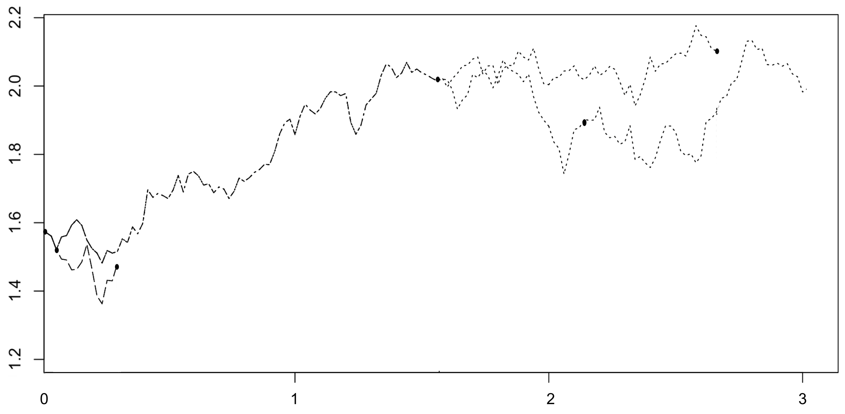
Figure 1: A typical simulated path of the branching diffusion starting from $\pi/2$ on $[0,3]$. Bullets denote branching or killing times.

To estimate the driver $\hat{f}$, we use a quadratic spline: on Figure 2 we plot $\hat{f}$ on $[0,1]\times[-\bar{y},\bar{y}]$ and the error obtained with a $20$ splines representation.

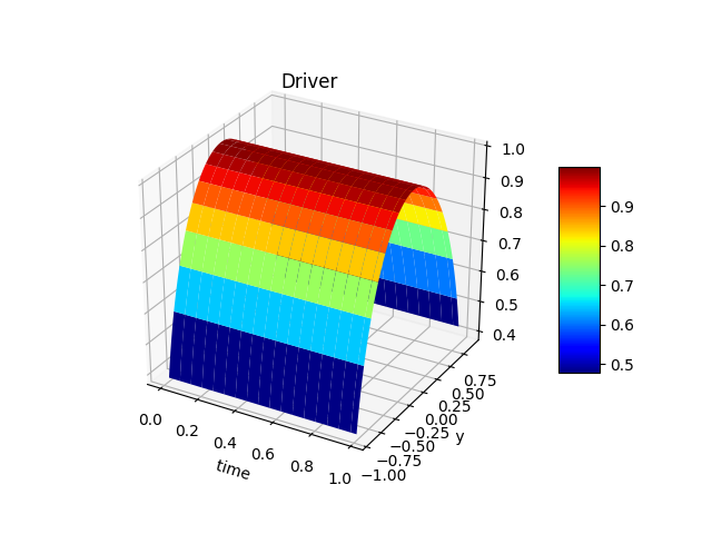
The driver

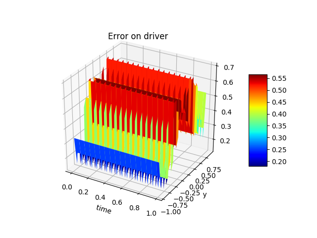
Error on the driver due to the spline representation.

Figure 2: The driver $\hat{f}$ and its quadratic spline representation error for 20 splines.

Notice that this driver has a high Lipschitz constant around $-\bar{y}$ and $\bar{y}$.

As already mentionned, we do not try to optimize the local polynomial representation, but instead generate the splines automatically. Our motivation is that the method should work in an industrial context, in which case a hand-made approximation might be complex to construct. Note however that one could indeed, in this test case, already achieve a very good precision with only three local polynomials as shown in Figure 3. Recalling Remark 2.10, this particular approximation would certainly be more efficient, in particular if the probability of reaching the boundary points, at which the precision is not fully satisfactory, is small.

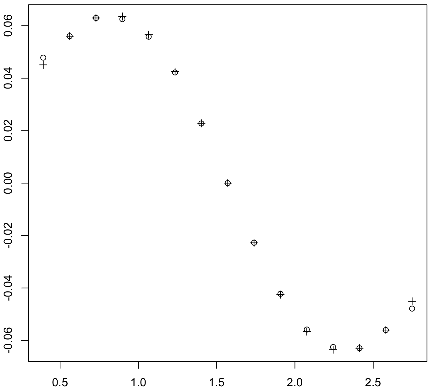
Figure 3: Approximation of the driver at $t=T$ with only three local polynomials - Crosses: $f(\cdot,\cos)$. Circles: $f_{\ell_{\circ}}(\cdot,\cos,\cos)$.

In Figure 4, we give the results obtained by method A for different values of $N_{h}$, the number of time steps, and of the number of splines used to construct $\hat{f}$. As shown on the graph, the error with $N_{h}=20$ and $20$ splines is below $0.004$, and even with $5$ time steps the results are very accurate. Besides the results obtained are very stable with the number of splines used.

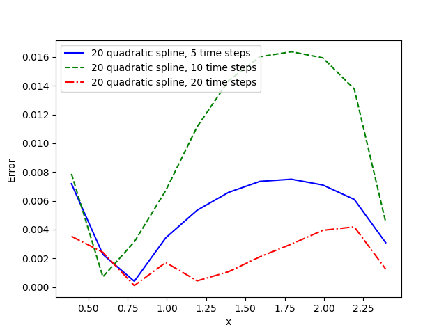
Error in absolute value for different
time discretization.

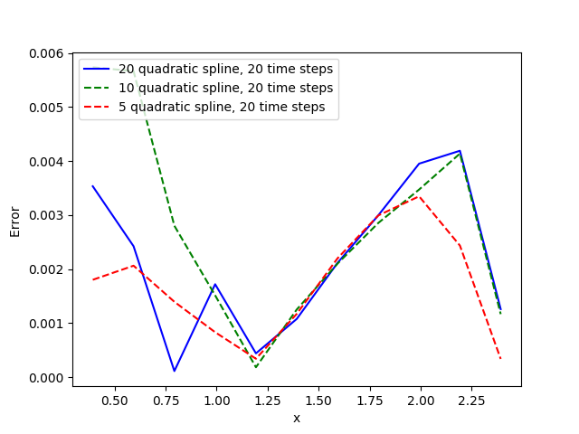
Error in absolute value for different
number of splines.

Figure 4: Results for the toy case using method A

On Figure 5, we give the results obtained with the method B for different values of $N_{h}$ and $\hat{N}_{h}$ keeping the number $N_{h}\hat{N}_{h}$ constant, equal to $20$.

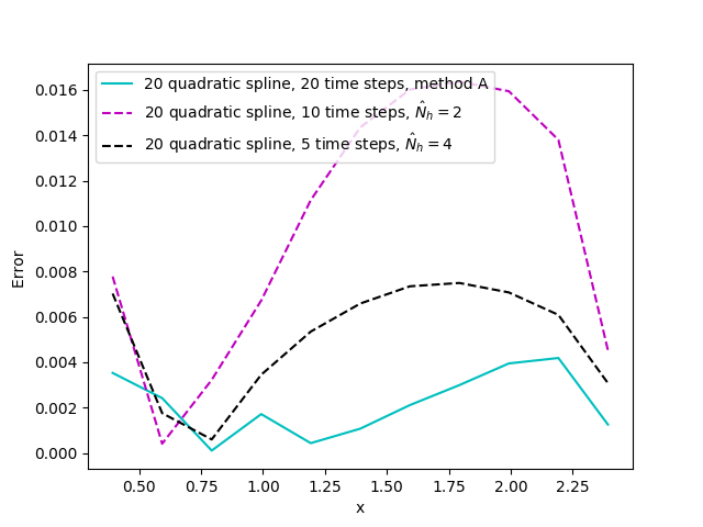
Figure 5: Error in absolute value for method B for different $N_{h}$ and $\hat{N}_{h}$, keeping $N_{h}\hat{N}_{h}=20$.

Comparing Figure 4 and Figure 5, we see that the results obtained with the two methods are similar, for a same total number of time steps. This shows that method B is less efficient, as it gives similar results but at the cost of additional computations. This is easily explained by the fact that the variance increases a lot with the size of the time step, so as to become the first source of error. In the sequel of the article, we will therefore concentrate on method A.
The time spent for the best results, obtained with method A, $20$ time steps and $20$ splines, is less than $1.05$ seconds on a regular (old indeed) laptop.

3.2 Some more difficult examples

We show in this section that the method works well even in more difficult situations, in particular when the boundary condition $g$ is not bounded by one. This will be at the price of a higher variance, that is compensated by an increase of the computational cost.
We now take $\mathbf{X}:=[0,2]^{d}$, with

$$\mu(x)=U\times({\bf 1}-x)\;\mbox{ and }\;\sigma(x):=V\prod_{i=1}^{d}(2-x_{i})x_{i}{\rm I_{d}},$$

where $V=0.2$, $U=0.1$ and ${\rm I_{d}}$ is the identity matrix.

We will describe the drivers later on. Let us just immediatly mention that we use the modified monotonic quadratic interpolator defined in [27] for tensorized interpolations in dimension $d$. When using sparse grids, we apply the quadratic interpolator of [8]. The spatial discretization used for all tests is defined with

• a step 0.2 for the full grid interpolator,

• a level 4 for the sparse grid interpolator [7].

We take a very thin time step of $0.000125$ for the Euler scheme of $X$. The number of simulations $\hat{M}$ is chosen such ${\theta}/{\sqrt{\hat{M}}}<0.00025$ and limited to $200.000$, so that the error reached can be far higher than $0.00025$ for high time steps. This is due to fact that the empirical standard deviation $\theta$ is large for some points near the boundary of $\mathbf{X}$. We finally use a truncation parameter $M=50$, it does not appear to be very relevant numerically.

3.2.1 A first one dimensional example

In this part, we use the following time dependent driver for a first one dimensional example:

$$f(t,y)= y(\frac{1}{2}-\frac{V^{2}}{2C^{2}}[\phi(t,T,y)(2C-\phi(t,T,y))]^{2}-U(C-\phi(t,T,y))),$$

with $\phi(t,T,y)=\log(y)-\frac{T-t}{2}.$
We use a time discretization of $1.000$ time steps to represent the time dependency of the driver. On Figure 6, we provide the driver and the cubic spline error associated to 10 splines.

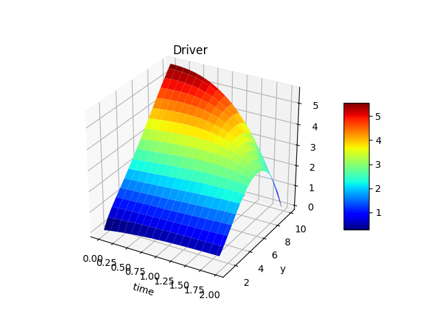
The driver

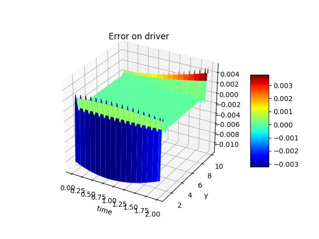
Error on the driver due to the spline representation.

Figure 6: The driver and its cubic spline representation error with 10 splines for the first difficult case.

Figure 8 corresponds to cubic splines (with an approximation on each mesh with a polynomial of degree 3), while Figure 8 corresponds to quadratic splines (with an approximation on each mesh with a polynomial of degree 2).

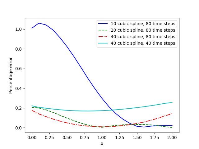
Figure 7: Cubic spline method.

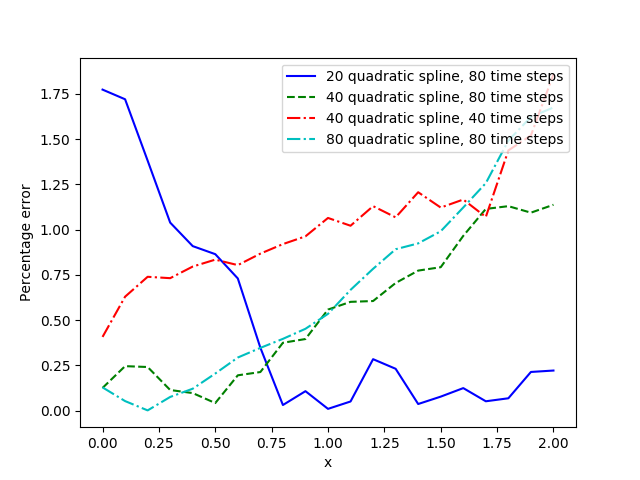
Figure 8: Quadratic spline method.

Percentage error on the approximation of the solution $v(0,.)$ for different time discretization and spline discretization.

On this example, the cubic spline approximation appears to be far more efficient than the quadratic spline. In order to get a very accurate solution when using sparse grids, with a maximum error below $0.2\%$, it is necessary to have a high number of splines (at least $20$) and a high number of time steps, meaning that the high variance of the method for the highest time step has prevented the algorithm to converge with the maximum number of samples imposed.

3.2.2 A second one dimensional example

We now consider the driver

$$f(x,y)=f_{1}(y)+f_{2}(x),$$ (24)

with

$$f_{1}(y)= \frac{2}{10}(y+\sin(\frac{\pi}{2}y)),$$ (25)

$$f_{2}(x)= \frac{1}{2}-(\frac{2}{10}+C\mu(x))-\frac{\sigma(x)^{2}c^{2}}{2}e^{Cx+\frac{T-t}{2}}-\frac{2}{10}\sin(\frac{\pi}{2}e^{cx+\frac{T-t}{2}}).$$

Figure 9 shows $f_{1}$ and the cubic spline error associated to different numbers of splines.

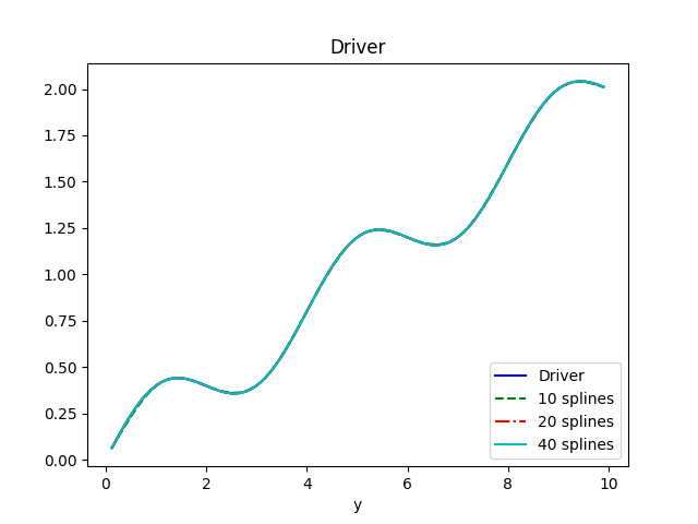
The driver

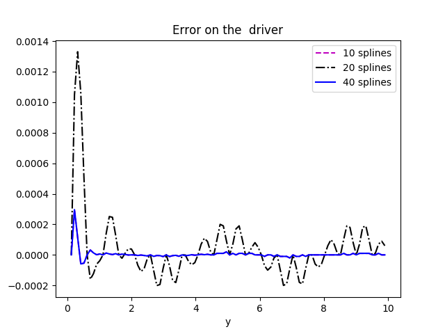
Error on the driver due to the spline representation.

Figure 9: The driver and its cubic spline representation.

On Figure 11 and 11, we give, in percentage, the error obtained when using cubic and quadratic splines for different discretizations.

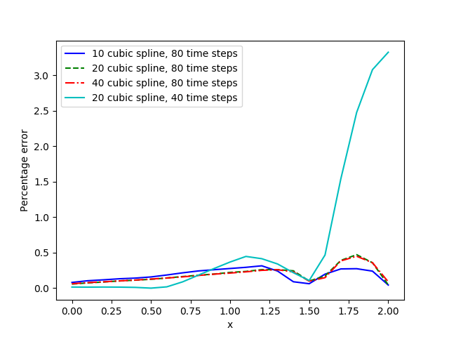
Figure 10: Cubic spline method.

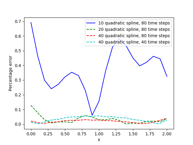
Figure 11: Quadratic spline method.

Percentage error on the aproximation of the solution $v(0,.)$ for different time discretizations and numbers of splines.

Globally, the quadratic interpolator appears to provide better results for both coarse and thin discretizations. With $40$ time steps, the cubic approximation generate errors up to $3\%$ at the boundary point $x=2$: reviewing the results at each time step, we checked that the convergence of the Monte Carlo is not achieved near the boundary $x=2$, with Monte Carlo errors up to $0.03$ at each step.

Finally, note that the convergence of the method is related to the value of the quadratic and cubic coefficients of the spline representation, that we want to be as small as possible.

3.2.3 Multidimensional results

In this section, we keep the driver in the form (24) with $f_{1}$ as in (25), but we now generalize the definition of $f_{2}$:

$$f_{2}(x)= \frac{1}{2}-(\frac{2}{10}+\frac{C}{d}\sum_{i=1}^{d}x_{i})-\frac{\sigma^{11}(x)^{2}c^{2}}{2d}e^{\frac{C}{d}\sum_{i=1}^{d}x_{i}+\frac{T-t}{2}}$$

$$-\frac{2}{10}\sin(\frac{\pi}{2}e^{\frac{C}{d}\sum_{i=1}^{d}x_{i}+\frac{T-t}{2}})$$

In this section, we only consider cubic splines.

3.2.3.1   Results with full grids

Figure 12 describes the results in dimension 2 for $80$ time steps and different numbers of splines. Once again the number of splines used is relevant for the convergence.

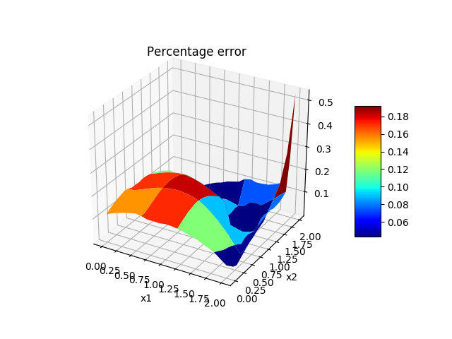
10 splines

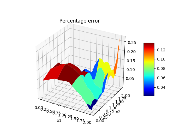
20 splines

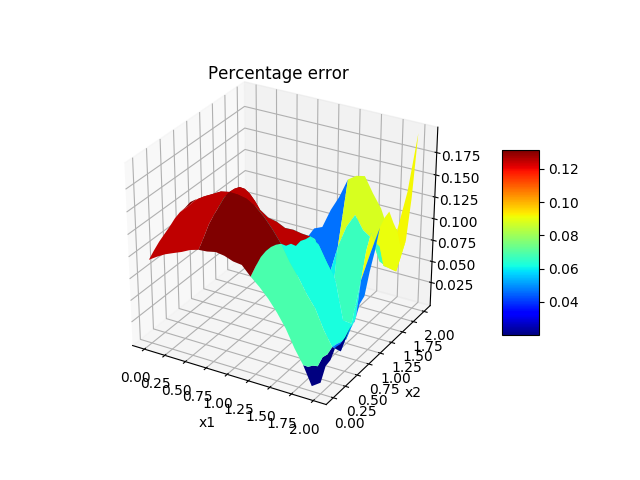
40 splines

Figure 12: Error in dimension 2 for $80$ time steps with cubic splines.

Figure 13 corresponds to dimension $3$ for different numbers of splines and different time discretizations: the error is plotted as a function of the point number using a classical Cartesian numeration. Once again, the results are clearly improved when we increase the number of splines and increase the number of time steps.

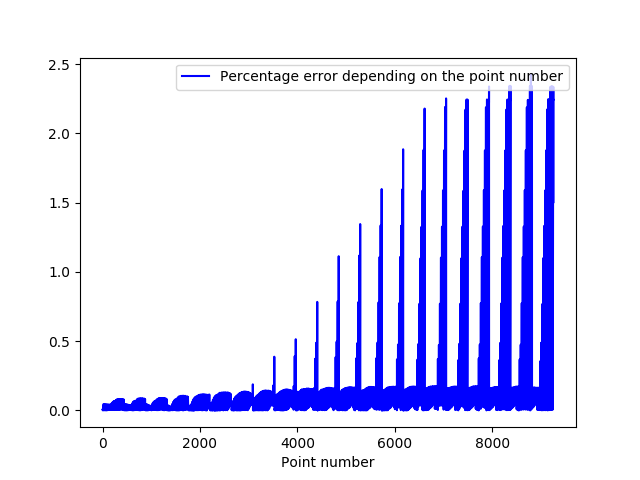
40 splines, 80 time steps.

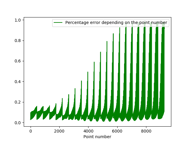
80 splines, 80 time steps

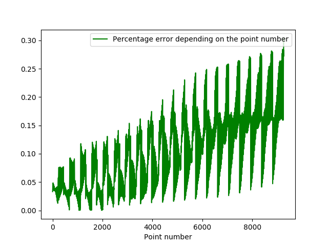
80 splines, 120 time steps

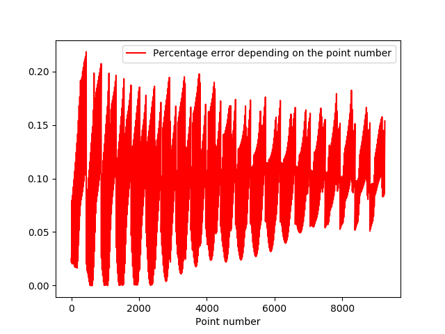
80 splines, 160 time steps

Figure 13: Error in dimension 3 for different time steps and spline numbers, with cubic splines.

3.2.3.2   Towards higher dimension

As the dimension increases, the algorithm is subject to the curse of dimensionality. This is due to the $d$-dimensional interpolation: the number of points used is $n^{d}$ if $n$ is the number of points in one dimension. One way to surround this is to use sparse grids [7]. The sparse grid methodology permits to get an interpolation error nearly as good as with full grids for a cost increasing slowly with the dimension, whenever the solution is smooth enough. It is based on some special interpolation points. According to [7, 8], if the function $w$ to be interpolated is null at the boundary and admits derivatives such that $\sup_{\alpha_{i}\in\{2,3\}}\left\{||\frac{\partial^{\alpha_{1}+..+\alpha_{d}}\;w}{\partial x_{1}^{\alpha_{1}}...\partial x_{d}^{\alpha_{d}}}||_{\infty}\right\}<\infty$, then the interpolation error due to the quadratic sparse interpolator $I^{2}$ is given

$$||w-I^{2}(w)||_{\infty}=O(n^{-3}log(n)^{d-1}).$$ (26)

An effective sparse grids implementation is given in [13] and more details on sparse grids can be found in [14].
On Figure 14, we plot the error obtained with a $2$-dimensional sparse grid, for $80$ time steps.

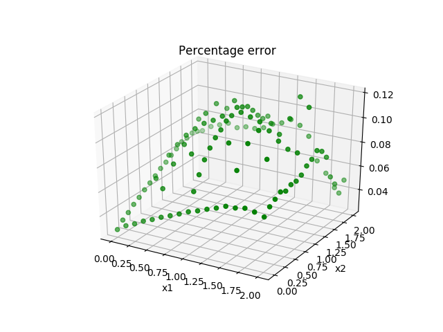
Figure 14: Error of the quadratic sparse grid of level 4 with 80 time steps

In dimension 3, 4, and 5, the error obtained with the spline of level 4 is given in Figure 15. Once again, we are able to be very accurate.

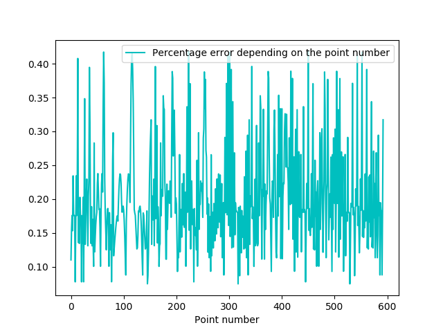
3D, 80 splines, 160 time steps.

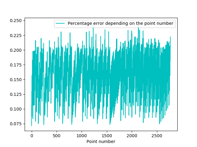
4D, 80 splines, 120 time steps.

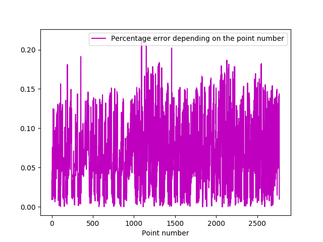
4D, 80 splines, 160 time steps.

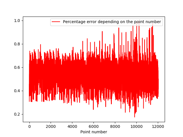
5D , 80 splines, 160 time steps.

Figure 15: Error in dimensions 3, 4 and 5 with a cubic spline approximation and a quadratic sparse interpolator.

Remark 3.2.

On Figure 15, the error is plotted as a function of the point number. Due to the special structure of the sparse grid points numeration, no special pattern appears (as on Figure 13) but the maximum error is still located at the boundary of $\mathbf{X}$.

From a practical point of view, the algorithm can be easy parallelized: at each time step each, points can be affected to one processor. It can therefore be speeded-up (linearly) with respect to the number of cores used.

All results have been obtained using a cluster with a MPI implementation for the parallelization. The time spend using the sparse grid interpolator in 3D, a Monte Carlo accuracy fixed to $0.0005$ and for an Euler scheme with time step $0.001$, is $2.800$ seconds on a cluster with 8 processors using 112 cores. The error curve can be found in Figure 16.

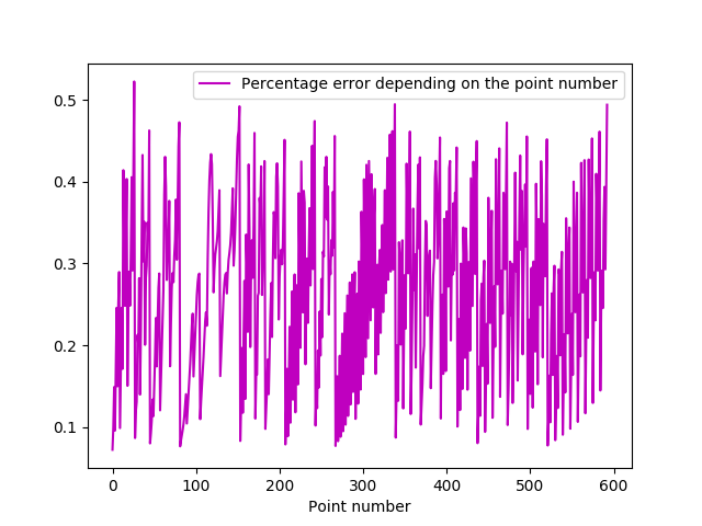
Figure 16: Error in dimension 3, 80 splines, 160 time steps and less tight parameters.

Remark 3.3.

When the solution has not the required regularity to reach the interpolation error (26), one can implement a local adaptation of the grid using a classical estimation of the local error (based on the hierarchical surplus) [16, 7]. It is also possible to use the dimension adaptive method [12], which aims at refining a whole dimension when a higher interpolation error in this dimension is detected.

Remark 3.4.

The methodology developed here is very similar in spirit to the Semi-Lagrangian method used in [27, 28] using full or sparse grids: the deterministic scheme starting from one point of the grid is replaced by a Monte Carlo one. Classically, the error of such a scheme is decomposed into a time discretization error and an interpolation error. This is the same in our scheme but, to the time discretization error due to the use of the scheme (22), is added a Monte Carlo error associated to the branching scheme.

Appendix A Appendix

A.1 Technical lemmas

Lemma A.1.

The ordinary differential equation $\eta^{\prime}(t)=\sum_{\ell=0}^{\ell_{\circ}}2C_{\ell_{\circ}}\eta(t)^{\ell}$ with initial condition $\eta(0)=M>0$ has a unique solution on $[0,h_{\circ}]$ for

$$h_{\circ}:=\frac{(\ell_{\circ}-1)(1-M)_{+}+(1\vee M)^{-(\ell_{\circ}-1)}}{(\ell_{\circ}+1)(\ell_{\circ}-1)2C_{\ell_{\circ}}}.$$ (27)

Moreover, it is bounded on $[0,h_{\circ}]$ by

$$M_{h_{\circ}}:=\max\!\Big{(}1,\big{(}(1\vee M)^{1-\ell_{\circ}}\!+\!(\ell_{\circ}\!-\!1)(1\!-\!M)^{+}\!-\!h_{\circ}\ell_{\circ}(\ell_{\circ}\!-\!1)2C_{\ell_{\circ}}\big{)}^{(1-\ell_{\circ})^{-1}}\Big{)}.$$ (28)

Consequently, one has, for all $t\in[0,h_{\circ}]$,

$$\mathbb{E}\Big{[}\Big{(}\prod_{k\in{\cal K}_{t}}\frac{M}{\bar{F}(t-T_{k-})}\Big{)}\Big{(}\prod_{k\in\bar{\cal K}_{t}\setminus{\cal K}_{t}}\frac{2C_{\ell_{\circ}}}{p_{\xi_{k}}\rho(\delta_{k})}\Big{)}\Big{]}~{}\leq~{}\eta(t)~{}\leq~{}M_{h_{\circ}}.$$ (29)

Proof. $\mathrm{i)}$ We first claim that

$$\int_{M}^{M_{h_{\circ}}}\frac{dy}{2C_{\ell_{\circ}}(1+y+\cdots+y^{\ell_{\circ}})}\geq h_{\circ}.$$ (30)

Then, for every $t\in[0,h_{\circ}]$, there is some constant $M(t)\leq M_{h_{\circ}}<\infty$ such that

$$\int_{M}^{M(t)}\frac{dy}{2C_{\ell_{\circ}}(1+y+\cdots+y^{\ell_{\circ}})}~{}=~{}t=\int_{0}^{t}ds.$$

This means that $(M(t))_{t\in[0,h_{\circ}]}$ is a bounded solution (and hence the unique solution) of $\eta^{\prime}(t)=\sum_{\ell=0}^{\ell_{\circ}}2C_{\ell_{\circ}}\eta(t)^{\ell}$ with initial condition $\eta(0)=M>0$. In particular, it is bounded by $M_{h_{\circ}}$.

$\mathrm{ii)}$ Let us now prove (30). Notice that $y^{k}\leq 1\vee y^{\ell_{\circ}}$ for any $y\geq 0$ and $k=0,\cdots,\ell_{\circ}$. Then, it is enough to prove that

$$\int_{M}^{M_{h_{\circ}}}\Big{(}1\wedge\frac{1}{y^{\ell_{\circ}}}\Big{)}dy\geq h_{\circ}(\ell_{\circ}+1)2C_{\ell_{\circ}}.$$ (31)

By direct computation, the l.h.s. of (31) equals

$$(M_{h_{\circ}}-M){\bf 1}_{\{M_{h_{\circ}}\leq 1\}}+\Big{(}(1-M)^{+}+\frac{1}{\ell_{\circ}-1}\big{(}(1\vee M)^{1-\ell_{\circ}}-M_{h_{\circ}}^{1-\ell_{\circ}}\big{)}\Big{)}{\bf 1}_{\{M_{h_{\circ}}>1\}}.$$

When $h_{\circ}$ satisfies (27), it is easy to check that (31) holds true.

$\mathrm{iii)}$ We now prove (29). Recall that $\bar{\cal K}_{t}^{n}$ denotes the collection of all particles in $\bar{\cal K}_{t}$ of generation $n$. Set

$$\chi^{n}_{t}:=\Big{(}\prod_{k\in\cup_{j=1}^{n}{\cal K}^{j}_{t}}\frac{M}{\bar{F}(t-T_{k-})}\Big{)}\Big{(}\prod_{k\in\cup_{j=1}^{n}(\bar{\cal K}^{j}_{t}\setminus{\cal K}^{j}_{t})}\frac{2C_{\ell_{\circ}}}{p_{\xi_{k}}\rho(\delta_{k})}\Big{)}\Big{(}\prod_{k\in\bar{\cal K}^{n+1}_{t}}\eta(t-T_{k-})\Big{)}.$$

Since $\bar{\cal K}^{n}_{t}$ has only finite number of particles, the random variable $\chi^{n}_{t}$ is uniformly bounded. Then by exactly the same arguments as in (32) and (A.1) below, and by repeating this argument over $n$, one has

$$\eta(t)=M+\int_{0}^{t}\sum_{\ell=0}^{\ell_{\circ}}2C_{\ell_{\circ}}\eta(s)^{\ell}ds=\mathbb{E}\big{[}\chi^{1}_{t}\big{]}=\mathbb{E}\big{[}\chi^{n}_{t}\big{]},~{}~{}~{}\forall n\geq 1.$$

It follows by Fatou Lemma that

$$\mathbb{E}\Big{[}\Big{(}\prod_{k\in{\cal K}_{t}}\frac{M}{\bar{F}(t-T_{k-})}\Big{)}\Big{(}\prod_{k\in\bar{\cal K}_{t}\setminus{\cal K}_{t}}\frac{2C_{\ell_{\circ}}}{p_{\xi_{k}}\rho(\delta_{k})}\Big{)}\Big{]}=\mathbb{E}\big{[}\lim_{n\to\infty}\chi^{n}_{t}\big{]}~{}\leq~{}\lim_{n\to\infty}\mathbb{E}[\chi^{n}_{t}]=\eta(t).$$

∎

For completeness, we provide here the proof the representation formula of Proposition 2.5 and of the technical lemma that was used in the proof of Proposition 2.8.

Proposition A.2.

The representation formula of Proposition 2.5 holds.

Proof. We only provide the proof on $[t_{N_{h}-1},T]$, the general result is obtained by induction. It is true by construction when $m$ is equal to $0$. Let us now fix $m\geq 1$.

First, Lemma A.1 shows that the random variable $V^{m}_{t,x}$ is integrable.

Next, Set $(1)+:=\{(1,j),j\leq\ell_{\circ}\}\cap\bar{\cal K}_{T}$ and define ${\cal K}_{t}(1):={\cal K}_{t}\cap(1)+$ and $\bar{\cal K}_{t}(1):=\bar{\cal K}_{t}\cap(1)+$. For ease of notations, we write $X^{x}:=X^{x,((1))}$. Then, for all $(t,x)\in[t_{N_{h}-1},T]\times\mathbb{R}^{d}$,

$$\mathbb{E}[V^{m}_{t,x}] =\mathbb{E}\left[\frac{g(X_{T-t}^{x})}{\bar{F}(T-t)}{\bf 1}_{\{T_{(1)}\geq T-t\}}\right]$$

$$+\mathbb{E}\left[{\bf 1}_{\{T_{(1)}<T-t\}}\frac{\sum_{j=1}^{j_{\circ}}a_{j,\xi_{(1)}}(X_{T_{(1)}}^{x})\varphi_{j}(v^{m-1}(t+T_{(1)},X_{T_{(1)}}^{x}))}{p_{\xi_{(1)}}\,\rho(\delta_{(1)})}R^{m}_{t,x}\right]$$

where

$$R^{m}_{t,x}:=\Big{(}\prod_{k\in{\cal K}_{T-t}(1)}G_{t,x}(k)\Big{)}\Big{(}\prod_{k\in\bar{{\cal K}}_{T-t}(1)\setminus{\cal K}_{T-t}(1)}A^{m}_{t,x}(k)\Big{)}$$

satisfies

$$\mathbb{E}[R^{m}_{t,x}|{\cal F}_{T_{(1)}}]=\prod_{k\in(1)+}v^{m}\big{(}{t+}T_{(1)},X^{t,x}_{T_{(1)}}\big{)}=\big{[}v^{m}({t+}T_{(1)},X^{x}_{T_{(1)}})\big{]}^{\xi_{(1)}},$$

by (17). On the other hand, (16) and (17) imply

$$\mathbb{E}\left[\frac{g(X_{T-t}^{x})}{\bar{F}(T-t)}{\bf 1}_{\{T_{(1)}\geq T-t\}}\right] =\mathbb{E}[g(X_{T-t}^{x})]$$ (32)

and

$$\mathbb{E}\left[{\bf 1}_{\{T_{(1)}<T-t\}}\frac{\sum_{j=1}^{j_{\circ}}a_{j,\xi_{(1)}}(X_{T_{(1)}}^{x})\varphi_{j}(v^{m-1}(t+T_{(1)},X_{T_{(1)}}^{x}))}{p_{\xi_{(1)}}\,\rho(\delta_{(1)})}[v^{m}({t+}T_{(1)},X^{x}_{T_{(1)}})]^{\xi_{(1)}}\right]$$

$$=\mathbb{E}\left[\int_{0}^{T-t}\frac{\sum_{j=1}^{j_{\circ}}a_{j,\xi_{(1)}}(X^{x}_{s})\varphi_{j}(v^{m-1}(t+s,X_{s}^{x}))}{p_{\xi_{(1)}}}[v^{m}({t+}s,X^{x}_{s})]^{\xi_{(1)}}ds\right]$$

$$=\mathbb{E}\left[\int_{0}^{T-t}\sum_{j=1}^{j_{\circ}}\sum_{\ell\leq\ell_{\circ}}a_{j,\ell}(X_{{s}}^{x})\varphi_{j}(v^{m-1}(t+s,X_{{s}}^{x}))[v^{m}({t+}s,X^{x}_{s})]^{\ell}ds\right]$$

$$=\mathbb{E}\left[\int_{0}^{T-t}f_{\ell_{\circ}}(X_{{s}}^{x},v^{m}(t+s,X_{{s}}^{x}),v^{m-1}(t+s,X_{{s}}^{x}))ds\right].$$ (33)

Combining the above implies that

$$v^{m}(t,X_{t})=\mathbb{E}\left[g(X_{T})+\int_{t}^{T}f_{\ell_{\circ}}(X_{s},v^{m}(s,X_{s}),v^{m-1}(s,X_{s}))ds\Big{|}{\cal F}_{t}\right],$$

and the required result follows by induction. $\Box$

Lemma A.3.

Let $(x^{i},y^{i})_{i\leq I}$ be a sequence of real numbers. Then,

$$\left|\prod_{i=1}^{I}x^{i}-\prod_{i=1}^{I}y^{i}\right|\leq\sum_{i\in I}\Big{(}|x^{i}-y^{i}|\prod_{j\neq i}\max(|x^{j}|,|y^{j}|)\Big{)}.$$

Proof. It suffices to observe that

$$\prod_{i=1}^{I}x^{i}-\prod_{i=1}^{I}y^{i}~{}=~{}(x^{1}-y^{1})\prod_{i=2}^{I}x^{i}+y^{1}\Big{(}\prod_{i=2}^{I}x^{i}-\prod_{i=2}^{I}y^{i}\Big{)},$$

and to proceed by induction. $\Box$

Proposition A.4.

Let $c_{1},c_{2},c_{3}\geq 0$, and let $(u^{i}_{m})_{m\geq 0,i\geq 0}$ be a sequence such that

$$u^{i}_{m}\leq c_{1}u^{i}_{m-1}+c_{2}u^{i+1}_{m}+c_{3}\;\mbox{ for }m\geq 1,i<N_{h}.$$

Then

$$u^{i}_{m}\leq c_{1}^{m}u^{i}_{0}+\sum_{i^{\prime}=1}^{N_{h}-i}\left(\sum_{j_{1}=1}^{m}\sum_{j_{2}=1}^{j_{1}}\cdots\sum_{j_{i^{\prime}}=1}^{j_{i^{\prime}-1}}c_{1}^{m}c_{2}^{i^{\prime}}u^{i+i^{\prime}}_{0}\right)$$

$$+c_{3}\left(\sum_{i=1}^{m}c^{i}_{1}+\sum_{i^{\prime}=2}^{N_{h}-i}\Big{(}\sum_{j_{1}=1}^{m}\sum_{j_{2}=1}^{j_{1}}\cdots\sum_{j_{i^{\prime}}=1}^{j_{i^{\prime}-1}}c_{1}^{m-j_{i^{\prime}}}c_{2}^{i^{\prime}-1}\Big{)}\right).$$

Proof. We have

$$u^{i}_{m}\leq (c_{1})^{m}u^{i}_{0}+\sum_{j=1}^{m}(c_{1})^{m-j}(c_{2}u^{i+1}_{m}+c_{3}).$$

The required result then follows from a simple induction. $\Box$

A.2 More on the error analysis for the abstract numerical approximation

The regression error ${\cal E}(\hat{\mathbb{E}})$ in Assumption 2.6 depends essentially on the regularity of $v^{m}$. Here we prove that $v^{m}(t,x)$ is Hölder in $t$ and Lipschitz in $x$ under additional conditions, and provide some estimates on the corresponding coefficients. Given $\phi:[0,T]\times\mathbb{R}^{d}\to\mathbb{R}$, denote

$$[\phi]_{{t_{i}}}~{}:=~{}\sup_{(t,x)\neq(t^{\prime},x^{\prime})\in[{t_{i}},{t_{i+1}}]\times\mathbf{X}}\frac{|\phi(t,x)-\phi(t^{\prime},x^{\prime})|}{|t-t^{\prime}|^{\frac{1}{2}}+|x-x^{\prime}|}.$$

Since $(\mu,\sigma)$ is assumed to be Lipschitz, it is clear that there exists $L_{X}>0$ such that for all $(t,x),(t^{\prime},x^{\prime})\in[0,T]\times\mathbf{X}$,

$$\|X^{x}_{t}-X^{x^{\prime}}_{t^{\prime}}\|_{{\mathbf{L}}^{2}}\leq L_{X}\Big{(}\sqrt{|t^{\prime}-t|}+|x^{\prime}-x|\Big{)}.$$ (34)

Proposition A.5.

Suppose that $x\mapsto g(x)$ and $x\mapsto f_{\ell_{\circ}}(x,y,y^{\prime})$ are uniformly Lipschitz with Lipschitz constants $L_{g}$ and $L_{f}$. Let $\beta$ and $\lambda_{1},\lambda_{2}>0$ such that $\frac{L_{2}}{\lambda^{2}_{2}}T<1$ and $\beta\geq 2L_{1}+L_{f}\lambda_{1}^{2}+L_{2}\lambda^{2}_{2}$, then for all $m\geq 1$ and $i\leq N_{h}$,

$$[v^{m}]_{{t_{i}}}~{}\leq~{}L_{v} := (1+L_{X})L_{X}\sqrt{\big{(}L_{g}^{2}+\frac{L_{f}}{\beta\lambda^{2}_{1}}\big{)}e^{\beta T}/\big{(}1-\frac{L_{2}}{\lambda_{2}^{2}}T\big{)}}$$

$$+~{}2(1+\ell_{\circ})C_{\ell}(1\vee(M_{h_{\circ}})^{\ell_{\circ}})\sqrt{h_{\circ}}.$$

Proof. For ease of notations, we provide the proof for $t=0$ only.

$\mathrm{i)}$ Let $x_{1},x_{2}\in\mathbb{R}^{d}$ and $Y^{m,1}:=v^{m}(\cdot,X^{x_{1}})$, $Y^{m,2}:=v^{m}(\cdot,X^{x_{2}})$, and denote $\Delta Y^{m}:=Y^{m,1}-Y^{m,2}$, $\Delta X:=X^{x_{1}}-X^{x_{2}}$, where $X^{x_{1}}$ (resp. $X^{x_{2}}$) denotes the solution of SDE (2) with initial condition $X_{0}=x_{1}$ (resp. $X_{0}=x_{2}$). Using the same arguments as in the proof of Theorem 2.4, it follows that, for any $\beta\geq 2L_{1}+L_{f}\lambda_{1}^{2}+L_{2}\lambda^{2}_{2}$, one has

$$\mathbb{E}[e^{\beta t}(\Delta Y_{t}^{m+1})^{2}] \leq \mathbb{E}[e^{\beta T}(\Delta Y_{T}^{m+1})^{2}]~{}+~{}\frac{L_{f}}{\lambda_{1}^{2}}\mathbb{E}\Big{[}\int_{t}^{T}e^{\beta s}|\Delta X_{s}|^{2}ds\Big{]}$$ (35)

$$+\frac{L_{2}}{\lambda^{2}_{2}}\mathbb{E}\Big{[}\int_{t}^{T}e^{\beta s}(\Delta Y^{m}_{s})^{2}ds\Big{]}$$

and then

$$\mathbb{E}\Big{[}\int_{0}^{T}e^{\beta t}(\Delta Y^{m+1}_{t})^{2}dt\Big{]} \leq T\mathbb{E}[e^{\beta T}(\Delta Y_{T}^{m+1})^{2}]+T\frac{L_{f}}{\lambda_{1}^{2}}\mathbb{E}\Big{[}\int_{0}^{T}e^{\beta s}|\Delta X_{s}|^{2}ds\Big{]}$$

$$+~{}T\frac{L_{2}}{\lambda_{2}^{2}}\mathbb{E}\Big{[}\int_{0}^{T}e^{\beta t}(\Delta Y^{m}_{t})^{2}dt\Big{]}$$

$$\leq Te^{\beta T}\Big{(}L_{g}^{2}+\frac{L_{f}}{\beta\lambda_{1}^{2}}\Big{)}L_{X}^{2}|x_{1}-x_{2}|^{2}$$

$$+~{}T\frac{L_{2}}{\lambda_{2}^{2}}\mathbb{E}\Big{[}\int_{0}^{T}e^{\beta t}(\Delta Y^{m}_{t})^{2}dt\Big{]}.$$

Since $\frac{L_{2}}{\lambda^{2}_{2}}T<1$, this induces that

$$\mathbb{E}\Big{[}\int_{0}^{T}e^{\beta t}(\Delta Y^{m+1}_{t})^{2}dt\Big{]}~{}\leq~{}\frac{Te^{\beta T}\big{(}L_{g}^{2}+\frac{L_{f}}{\beta\lambda^{2}_{1}}\big{)}L_{X}^{2}|x_{1}-x_{2}|^{2}}{1-\frac{L_{2}}{\lambda^{2}_{2}}T}.$$

Plugging the above estimates into (35), it follows that

$$(\Delta Y_{0}^{m})^{2}~{}\leq~{}\hat{L}_{v}^{2}|x_{1}-x_{2}|^{2},~{}~{}~{}\mbox{with}~{}~{}\hat{L}_{v}^{2}:=\frac{\big{(}L_{g}^{2}+\frac{L_{f}}{\beta\lambda^{2}_{1}}\big{)}L_{X}^{2}e^{\beta T}}{1-\frac{L_{2}}{\lambda^{2}_{2}}T}.$$

$\mathrm{ii)}$ For the Hölder property of $v^{m}$, it is enough to notice that for $t\leq h_{\circ}$,

$$|v^{m}(0,x)-v^{m}(t,x)| \leq \mathbb{E}\Big{[}|v^{m}(t,X^{x}_{t})-v^{m}(t,x)|+\int_{0}^{t}|f(X^{x}_{s},Y^{m}_{s},Y^{m-1}_{s})|ds\Big{]}$$

$$\leq \hat{L}_{v}L_{X}\sqrt{t}+2(1+\ell_{\circ})C_{\ell}(1\vee(M_{h_{\circ}})^{\ell_{\circ}})t,$$

where the last inequality follows from the Lipschitz property of $v^{m}$ in $x$ and the fact that $Y^{m}$ is uniformly bounded by $M_{h_{\circ}}$. We hence conclude the proof. $\Box$

Ackowledgements

This work has benefited from the financial support of the Initiative de Recherche “Méthodes non-linéaires pour la gestion des risques financiers” sponsored by AXA Research Fund.

Bruno Bouchard and Xavier Warin acknowledges the financial support of ANR project CAESARS (ANR-15-CE05-0024).

Xiaolu Tan acknowledges the financial support of the ERC 321111 Rofirm, the ANR Isotace, and the Chairs Financial Risks (Risk Foundation, sponsored by Société Générale) and Finance and Sustainable Development (IEF sponsored by EDF and CA).

References

- [1] K. B. Athreya and P. E. Ney, Branching processes, Springer-Verlag, New York, 1972. Die Grundlehren der mathematischen Wissenschaften, Band 196.
- [2] V. Bally and P. Pages, Error analysis of the quantization algorithm for obstacle problems, Stochastic Processes & Their Applications, 106(1):1-40, 2003.
- [3] C. Bender and R. Denk. A forward scheme for backward SDEs, Stochastic Processes & Their Applications 117(12): 1793-1812, 2007.
- [4] M. Bossy, N. Champagnat, H. Leman, S. Maire, L. Violeau and M. Yvinec, Monte Carlo methods for linear and non-linear Poisson-Boltzmann equation, ESAIM:Proceedings and Surveys, 48:420-446, 2015.
- [5] B. Bouchard and N. Touzi, Discrete-time approximation and Monte-Carlo simulation of backward stochastic differential equations, Stochastic Process. Appl., 111(2):175-206, 2004.
- [6] B. Bouchard, X. Warin, Monte-Carlo valuation of American options: facts and new algorithms to improve existing methods. In Numerical methods in finance (pp. 215-255). Springer Berlin Heidelberg, 2012.
- [7] H.J. Bungartz, M. Griebel, Sparse Grids, Acta Numerica, volume 13, (2004), pp 147-269
- [8] H.-J. Bungartz, Concepts for higher order finite elements on sparse grids, Proceedings of the 3.Int. Conf. on Spectral and High Order Methods, pp. 159-170 , (1996)
- [9] J. Cvitanic, I. Karatzas. Backward stochastic differential equations with reflection and Dynkin games, The Annals of Probability, 2024-2056, 1996.
- [10] C. Deboor, A practical guide to splines, Springer-Verlag New York, 1978
- [11] N. El Karoui, S. Peng, M.C. Quenez, Backward stochastic differential equations in finance, Mathematical finance 7(1), 1-71, 1997.
- [12] T. Gerstner, M. Griebel ,Dimension-Adaptive Tensor-Product Quadrature, Computing 71, (2003) 89-114.
- [13] H. Gevret, J. Lelong, X. Warin , The StOpt library, https://gitlab.com/stochastic-control/StOpt
- [14] H. Gevret, J. Lelong, X. Warin , The StOpt library documentation, https://hal.archives-ouvertes.fr/hal-01361291
- [15] E. Gobet, J.P. Lemor, X. Warin, A regression-based Monte Carlo method to solve backward stochastic differential equations. The Annals of Applied Probability, 15(3):2172-202, 2005.
- [16] M. Griebel, Adaptive sparse grid multilevel methods for elliptic PDEs based on finite differences, Computing, 61(2):151-179,(1998)
- [17] P. Henry-Labordère, Cutting CVA’s Complexity, Risk magazine (Jul 2012).
- [18] P. Henry-Labordere, N. Oudjane, X. Tan, N. Touzi, X. Warin, Branching diffusion representation of semilinear PDEs and Monte Carlo approximation. arXiv preprint, 2016.
- [19] P. Henry-Labordere, X. Tan, N. Touzi A numerical algorithm for a class of BSDEs via the branching process. Stochastic Processes and their Applications. 28;124(2):1112-1140, 2014.
- [20] P.E. Kloeden and E. Platen, Numerical Solution of Stochastic Differential Equations, Stochastic Modelling and Applied Probability, Vol. 23, Springer, 1992.
- [21] H. P. McKean, Application of Brownian motion to the equation of Kolmogorov-Petrovskii-Piskunov, Comm. Pure Appl. Math., Vol 28, 323-331, 1975.
- [22] E. Pardoux and S. Peng, Adapted solutions of backward stochastic differential equations, System and Control Letters, 14, 55-61, 1990.
- [23] A. Rasulov, G. Raimova, M. Mascagni, Monte Carlo solution of Cauchy problem for a nonlinear parabolic equation, Mathematics and Computers in Simulation, 80(6), 1118-1123, 2010.
- [24] A.V. Skorokhod Branching diffusion processes, Theory of Probability & Its Applications, 9(3):445-449, 1964.
- [25] D. W. Stroock, S. R. S. Varadhan, Multidimensional Diffusion Processes, Springer, 1979.
- [26] G. Teschl, Ordinary Differential Equations and Dynamical Systems, American Mathematical Society, Graduate Studies in Mathematics, Volume 140, 2012.
- [27] X. Warin, Some Non-monotone Schemes for Time Dependent Hamilton-Jacobi-Bellman Equations in Stochastic Control, Journal of Scientific Computing, 66(3),1122-1147, 2016
- [28] X. Warin, Adaptive sparse grids for time dependent Hamilton-Jacobi-Bellman equations in stochastic control, arXiv preprint arXiv:1408.4267, 2014.
- [29] S. Watanabe, On the branching process for Brownian particles with an absorbing boundary, J. Math. Kyoto Univ. 4(2), 385-398, 1964.
- [30] J. Zhang, A numerical scheme for backward stochastic differential equations, Annals of Applied Probability, 14(1), 459-488, 2004.