Optimal Containment of Epidemics in Temporal and Adaptive Networks

Abstract

In this chapter, we focus on the problem of containing the spread of diseases taking place in both temporal and adaptive networks (i.e., networks whose structure ‘adapts’ to the state of the disease). We specifically focus on the problem of finding the optimal allocation of containment resources (e.g., vaccines, medical personnel, traffic control resources, etc.) to eradicate epidemic outbreaks over the following three models of temporal and adaptive networks: (i) Markovian temporal networks, (ii) aggregated-Markovian temporal networks, and (iii) stochastically adaptive models. For each model, we present a rigorous and tractable mathematical framework to efficiently find the optimal distribution of control resources to eliminate the disease. In contrast with other existing results, our results are not based on heuristic control strategies, but on a disciplined analysis using tools from dynamical systems and convex optimization.

1 Introduction

The containment of spreading processes taking place in complex networks is a major research area with applications in social, biological, and technological systems Watts1998 ; Newman2006 ; BBV08 . The spread of information in on-line social networks, the evolution of epidemic outbreaks in human contact networks, and the dynamics of cascading failures in the electrical grid are relevant examples of these processes. While major advances have been made in this field (see, for example, Nowzari2015a ; Pastor-Satorras2015a and references therein), most current results are specifically tailored to study spreading processes taking place in static networks. Cohen et al. CHB03 proposed a heuristic vaccination strategy called acquaintance immunization policy and proved it to be much more efficient than random vaccine allocation. In BCGS10 , Borgs et al. studied theoretical limits in the control of spreads in undirected network with a non-homogeneous distribution of antidotes. Chung et al. CHT09 studied a heuristic immunization strategy based on the PageRank vector of the contact graph. Preciado et al. PZEJP13 ; Preciado2014 studied the problem of determining the optimal allocation of control resources over static networks to efficiently eradicate epidemic outbreaks described by the networked SIS model. This work was later extended in PZ13 ; PSS13 ; PJ09 ; NPP14 ; XP14 ; NOPP15 ; WNPP15 ; Watkins2015 by considering more general epidemic models. Wan et al. developed in WRS08 a control theoretic framework for disease spreading, which has been recently extended to the case of sparse control strategies in TRW15 . Optimal control problems over networks have also been considered in KSA11 and KB14 . Drakopoulos et al. proposed in DOT14 an efficient curing policy based on graph cuts. Decentralized algorithms for epidemic control have been proposed in RM15 and in Trajanovski2015a using a game-theoretic framework to evaluate the effectiveness of protection strategies against SIS virus spreads. An optimization framework to achieve resource allocations that are robust to stochastic uncertainties in nodal activities was proposed in Ogura2015g .

Most epidemic processes of practical interest take place in temporal networks Masuda2013 , having time-varying topologies Holme2015b . In the context of temporal networks, we are interested in the interplay between the epidemiological dynamics on networks (i.e., the dynamics of epidemic processes taking place in the network) and the dynamics of networks (i.e., the temporal evolution of the network structure). Although the dynamics on and of networks are usually studied separately, there are many cases in which the evolution of the network structure is heavily influenced by the dynamics of epidemic processes taking place in the network. This can be illustrated by a phenomenon called social distancing Bell2006 ; Funk2010 , where healthy individuals avoid contact with infected individuals in order to protect themselves against the disease. As a consequence of social distancing, the structure of the network adapts to the dynamics of the epidemics taking place in the network. Similar adaptation mechanisms have been studied in the context of the power grid Scire2005 , biological systems Schaper2003 and on-line social networks Antoniades2013 .

We can find a plethora of studies dedicated to the analysis of epidemic spreading processes over temporal networks based on either extensive numerical simulations Vazquez2007 ; Karsai2011 ; Holme2014 ; Vestergaard2014 ; Masuda2013a ; Rocha2013a or rigorous theoretical analyses Volz2009 ; Schwarzkopf2010 ; Perra2012 ; Taylor2012 . However, there is a lack of methodologies for containing epidemic outbreaks on temporal networks (except the work Liu2014a for activity driven networks). This is also the case for adaptive networks. In this latter case, we find in the literature various methods for the analysis of the behavior of spreading processes evolving over adaptively changing temporal networks Gross2008 ; Rogers2012a ; Tunc2014 ; Guo2013 ; Valdez2012 ; Wang2011b ; Szabo-Solticzky2016 relying on extensive numerical simulations. However, this is a lack of effective control strategies in the context of adaptive networks.

Nevertheless, in recent years, we have witnessed an emerging effort towards the efficient containment of epidemic processes in temporal and adaptive networks using tools from the field of control theory. The aim of this chapter is to give an overview of this research thrust by focusing on optimal resource allocation problems for efficient eradication of epidemic outbreaks. We specifically focus the scope of this chapter on the following three classes of temporal and adaptive networks: 1) Markovian temporal networks Ogura2015a , 2) aggregated-Markovian edge-independent temporal networks Ogura2015c ; Nowzari2015b , and 3) adaptive SIS models Guo2013 ; Ogura2015i . We see that the optimal resource allocation problem in these three cases can be reduced to an efficiently solvable class of optimization problems called convex programs Boyd2004 (more precisely, geometric programs Boyd2007 ).

This chapter is organized as follows. After preparing necessary mathematical notations, in Section 2 we study the optimal resource allocation problem in Markovian temporal networks. We then focus our exposition on a specific class of Markovian temporal networks, called aggregated-Markovian edge-independent temporal networks, in Section 3. We finally present recent results in the context of adaptive SIS models in Section 4.

Notation

We denote the identity matrix by $I$. The maximum real part of the eigenvalues of a square matrix $A$ is denoted by $\lambda_{\max}(A)$. For matrices $A_{1}$, $\dotsc$, $A_{n}$, we denote by $\bigoplus_{i=1}^{n}A_{i}$ the block-diagonal matrix containing $A_{1}$, $\dotsc$, $A_{n}$ as its diagonal blocks. If the matrices $A_{1}$, $\dotsc$, $A_{n}$ have the same number of columns, then the matrix obtained by stacking $A_{1}$, $\dotsc$, $A_{n}$ in vertical is denoted by $\operatorname*{col}_{i=1}^{n}A_{i}$. An undirected graph is defined as the pair $\mathscr{G}=(\mathscr{V},\mathscr{E})$, where $\mathscr{V}=\{{1},\dotsc,{n}\}$ is a set of nodes and $\mathscr{E}$ is a set of edges, defined as unordered pairs of nodes. The adjacency matrix $A=[a_{ij}]_{i,j}$ of $\mathscr{G}$ is defined as the $n\times n$ matrix such that $a_{ij}=a_{ji}=1$ if $\{i,j\}\in\mathscr{E}$, and $a_{ij}=0$ otherwise.

2 Markovian Temporal Networks

Since the dynamics of realistic temporal networks has intrinsic uncertainties in, for example, the appearance/disappearance of edges, the durations of temporal interactions, and inter-event times, most mathematical models of temporal networks in the literature have been written in terms of stochastic processes. In particular, many stochastic models of temporal networks (see, e.g., Perra2012 ; Volz2009 ; Clementi2008 ; Karsai2014 ) employ Markov processes due to their simplicity, including time-homogeneity and memoryless properties. The aim of this section is to present a rigorous and tractable framework for the analysis and control of epidemic outbreaks taking place in Markovian temporal networks. We remark that, throughout this chapter, we shall focus on the specific type of spreading processes described by the networked SIS model among other networked epidemic models (see, e.g., Pastor-Satorras2015a ).

2.1 Model

In this subsection, we present the model of disease spread and temporal networks studied in this section. We start our exposition from reviewing a model of spreading processes over static networks called the Heterogeneous Networked SIS (HeNeSIS) model Preciado2014 , which is an extension of the popular $N$-intertwined SIS model VanMieghem2009a to the case of nodes with heterogeneous spreading rates. Let $\mathscr{G}$ be an undirected graph having $n$ nodes, where nodes in $\mathscr{G}$ represent individuals and edges represent interactions between them. At a given time $t\geq 0$, each node can be in one of two possible states: susceptible or infected. In the HeNeSIS model, when a node $i$ is infected, it can randomly transition to the susceptible state with an instantaneous rate $\delta_{i}>0$, called the recovery rate of node $i$. On the other hand, if a neighbor of node $i$ is in the infected state, then the neighbor can infect node $i$ with the instantaneous rate $\beta_{i}$, where $\beta_{i}>0$ is called the infection rate of node $i$. We define the variable $x_{i}(t)$ as $x_{i}(t)=1$ if node $i$ is infected at time $t$, and $x_{i}(t)=0$ if $i$ is susceptible; then, the transition probabilities of the HeNeSIS model in the time window $[t,t+h]$ can be written as

$$\Pr(x_{i}(t+h)=1\mid x_{i}(t)=0) =\beta_{i}\sum_{{j\in\mathscr{N}_{i}}}x_{j}(t)h+o(h),$$ (1)

$$\Pr(x_{i}(t+h)=0\mid x_{i}(t)=1) =\delta_{i}h+o(h),$$

where $\mathscr{N}_{i}$ is the set of neighbors of node $i$ and $o(h)/h\to 0$ as $h\to 0$.

Although the collection of variables $(x_{1},\dotsc,x_{n})$ is simply a Markov process, this process presents a total of $2^{n}$ possible states (two states per node). Therefore, its analysis is very hard for arbitrary contact networks of large size. A popular approach to simplify the analysis of this type of Markov processes is to consider upper-bounding linear models, as described below. Let $A$ denote the adjacency matrix of $\mathscr{G}$. Define the vector $p=(p_{1},\dotsc,p_{n})^{\top}$ and the diagonal matrices $P=\bigoplus(p_{1},\dotsc,p_{n})$, $B=\bigoplus(\beta_{1},\dotsc,\beta_{n})$, and $D=\bigoplus(\delta_{1},\dotsc,\delta_{n})$. Then, it is known Preciado2014 that the solutions $p_{i}(t)$ ($i=1$, $\dotsc$, $n$) of the vectorial linear differential equation

$$dp/dt=(BA-D)p$$ (2)

upper-bound the evolution of the infection probabilities $\Pr(\text{$i$ is infected at time $t$})$ from the exact Markov process with $2^{n}$ states. Thus, if the solution of (2) satisfies $p(t)\to 0$ exponentially fast as $t\to\infty$, then the infection dies out in the exact Markov process exponentially fast as well. Since the differential equation (2) is a linear system, the maximum real eigenvalue $\lambda_{\max}(BA-D)$ of the matrix $BA-D$ determines the asymptotic behavior of the solution. The above considerations show that the spreading process dies out exponentially fast if

$$\lambda_{\max}(BA-D)<0.$$ (3)

In the special case of homogeneous infection and recovery rates, i.e., $\beta_{i}=\beta$ and $\delta_{i}=\delta$ for all nodes $i$, condition (3) yields the following well-known extinction condition (see, e.g., Lajmanovich1976 ; Ahn2013 )

$$\frac{\beta}{\delta}<\frac{1}{\lambda_{\max}(A)}.$$ (4)

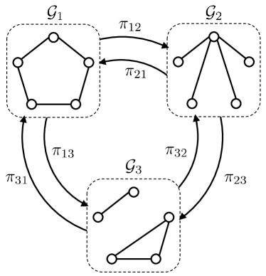
Figure 1: Markovian temporal network having three possible configurations ($\mathscr{G}_{1}$, $\mathscr{G}_{2}$, and $\mathscr{G}_{3}$), and the corresponding stochastic transition rates.

However, conditions (3) and (4) are not applicable to the case of temporal networks having time-varying adjacency matrices. In this section, we focus on the case where the dynamics of the temporal network is modeled by a Markov process. In order to specify a Markovian temporal network, we need the following two ingredients. The first one is the set of ‘graph configurations’ that can be taken by the temporal network of our interest. Let those configurations (static and undirected networks) be $\mathscr{G}_{1}$, $\dotsc$, $\mathscr{G}_{L}$. This implies that, at each time $t\geq 0$, the temporal network to be modeled always takes one of the configurations $\mathscr{G}_{1}$, $\dotsc$, $\mathscr{G}_{L}$. The other is the set of stochastic transition rates between graph configurations. Specifically, we let $\pi_{k\ell}$ denote the stochastic transition rate from the configuration $\mathscr{G}_{k}$ to $\mathscr{G}_{\ell}$. This implies that, if the configuration of the temporal network at time $t$ is $\mathscr{G}_{k}$, then the probability of the temporal network having another configuration $\mathscr{G}_{\ell}$ at time $t+h$ equals $\pi_{k\ell}h+o(h)$. We show a schematic diagram of a Markovian temporal network in Fig. 1.

We now describe the model of disease spread considered in this section. Let $\mathscr{G}(t)$ be a Markovian temporal network. Let $\mathscr{N}_{i}(t)$ be the set of neighbors of node $i$ at time $t$ in the graph $\mathscr{G}(t)$. Then, we can reformulate the transition probabilities (1) of the HeNeSIS model as

$$\Pr(x_{i}(t+h)=1\mid x_{i}(t)=0) =\beta_{i}\sum_{j\in\mathscr{N}_{i}(t)}x_{j}(t)h+o(h),$$ (5)

$$\Pr(x_{i}(t+h)=0\mid x_{i}(t)=1) =\delta_{i}h+o(h).$$

Notice that, in the first equation, the infection probability is dependent not only on the infection states of the other nodes but also the connectivity of the network. Then, we can formulate an upper-bounding model for the HeNeSIS model over the Markovian temporal network $\mathscr{G}(t)$ as

$$dp/dt=\left(BA(t)-D\right)p(t),$$ (6)

where $A(t)$ denotes the adjacency matrix of $\mathscr{G}(t)$.

2.2 Optimal Resource Distribution

Let us consider the following epidemiological problem Preciado2014 : Assume that we have access to vaccines that can be used to reduce the infection rates of individuals in the network, as well as antidotes that can be used to increase their recovery rates. Assuming that both vaccines and antidotes have an associated cost and that we are given a fixed budget, how should we distribute vaccines and antidotes throughout the individuals in the network in order to eradicate an epidemic outbreak at the maximum decay rate? In what follows, we state this question in rigorous terms and present an optimal solution using an efficient optimization framework called geometric programming Boyd2007 .

Assume that we have to pay $f(\beta_{i})$ unit of cost to tune the infection rate of node $i$ to $\beta_{i}$. Likewise, we assume that the cost for tuning the recovery rate of node $i$ to $\delta_{i}$ equals $g(\delta_{i})$. Notice that the total cost of tuning the collection of infection rates $(\beta_{1},\dotsc,\beta_{n})$ and recovery rates $(\delta_{1},\dotsc,\delta_{n})$ in the network is given by

$$R=\sum_{i=1}^{n}(f(\beta_{i})+g(\delta_{i})).$$

We further assume that these rates can be tuned within the following feasibility intervals:

$$0<\underaccent{\bar}{\beta}_{i}\leq\beta_{i}\leq\bar{\beta}_{i},\quad 0<\underaccent{\bar}{\delta}_{i}\leq\delta_{i}\leq\bar{\delta}_{i}.$$ (7)

We can now state our optimal resource allocation problem as follows:

Problem 1.

Consider a HeNeSIS spreading process over a Markovian temporal network. Given a budget $\bar{R}>0$, tune the infection and recovery rates $\beta_{i}$ and $\delta_{i}$ in the network in such a way that the exponential decay rate of the infection probabilities is maximized while satisfying the budget constraint $R\leq\bar{R}$ and the box constraints (7).

In order to solve this problem, we first present an analytical framework for quantifying the decay rate of the infection probabilities, given the parameters in the HeNeSIS model and the Markovian temporal network. In fact, using tools from control theory, it is possible to prove the following upper-bound on the decay rate of infection probabilities in the HeNeSIS model:

Proposition 1.

Consider the HeNeSIS spreading process over a Markovian temporal network. Let $\pi_{\ell\ell}=-\sum_{\ell\neq k}\pi_{\ell k}$. If

$$\lambda_{\max}(\mathscr{A}_{1})<0$$

for the matrix

$$\mathscr{A}_{1}=\begin{bmatrix}BA_{1}-D+\pi_{11}I&\ \pi_{21}I\ &\ \cdots\ &\pi_{L1}I\\ \rule{0.0pt}{17.22217pt}\pi_{12}I&\ \ddots\ &\ \ddots\ &\vdots\\ \rule{0.0pt}{17.22217pt}\vdots&\ \ddots\ &\ \ddots\ &\pi_{L,L-1}I\\ \rule{0.0pt}{17.22217pt}\pi_{1L}I&\ \cdots\ &\ \pi_{L-1,L}I\ &BA_{L}-D+\pi_{LL}I\end{bmatrix},$$

then the infection probabilities of nodes converge to zero exponentially fast with an exponential decay rate of $|\lambda_{\max}(\mathscr{A}_{1})|$.

Besides providing an analytical method for quantifying the rate of convergence to the disease-free state, this proposition allows us to sub-optimally minimize the decay rate of the epidemic outbreak by minimizing the maximum real eigenvalue $\lambda_{\max}(\mathscr{A}_{1})$ of the Metzler matrix $\mathscr{A}_{1}$. In fact, by employing the celebrated Perron-Frobenius theory Horn1990 for nonnegative matrices, we are able to solve Problem 1 via a class of optimization problems called geometric programs (Preciado2014, , Proposition 10), briefly reviewed below Boyd2007 . Let $x_{1}$, $\dotsc$, $x_{n}$ denote positive variables and define $x=(x_{1},\dotsc,x_{n})$. In the context of geometric programming, a real function $g(x)$ is a monomial if there exist a $c\geq 0$ and $a_{1},\dotsc,a_{n}\in\mathbb{R}$ such that $g(x)=cx_{\mathstrut 1}^{a_{1}}\dotsm x_{\mathstrut n}^{a_{n}}$. Also, we say that a function $f(x)$ is a posynomial if it is a sum of monomials of $x$ (we point the readers to Boyd2007 for more details). Given a collection of posynomials $f_{0}{(x)}$, $\dotsc$, $f_{p}{(x)}$ and monomials $g_{1}{(x)}$, $\dotsc$, $g_{q}{(x)}$, the optimization problem

$$\operatorname*{\text{minimize}}_{x>0} f_{0}(x)$$

$$\operatorname*{\text{subject to}} f_{i}(x)\leq 1,\quad i=1,\dotsc,p,$$

$$g_{j}(x)=1,\quad j=1,\dotsc,q,$$

is called a geometric program. A constraint of the form $f(x)\leq 1$ with $f(x)$ being a posynomial is called a posynomial constraint. It is known Boyd2007 that a geometric program can be efficiently converted into an equivalent convex optimization problem, which can be solved in polynomial time Boyd2004 .

We can now state the first main result of this chapter:

Theorem 2.1 ((Ogura2015a, , Section VI)).

Assume that the cost function $f$ is a posynomial and, also, there exists $\hat{\delta}>\bar{\delta}$ such that the function $\tilde{g}(\tilde{\delta})=g(\hat{\delta}-\tilde{\delta})$ is a posynomial in $\tilde{\delta}$. Then, the infection and recovery rates that solve Problem 1 are given by $\{\beta_{i}^{\star}\}_{i=1}^{n}$ and $\{\hat{\delta}-\tilde{\delta}_{i}^{\star}\}_{i=1}^{n}$, where the starred variables solve the optimization problem

$$\operatorname*{\text{minimize}}_{\beta_{i},\,\tilde{\delta}_{i},\,v>0,\,\lambda>0} 1/\lambda$$ (8)

subject to $$\mathscr{A}_{1}v\leq-\lambda v,$$

$${\sum_{i=1}^{n}(f(\beta_{i})+\tilde{g}(\tilde{\delta}_{i}))}\leq\bar{R},$$

$${\underaccent{\bar}{\beta}}\leq\beta_{i}\leq\bar{\beta},$$

$$\hat{\delta}-\bar{\delta}\leq\tilde{\delta}_{i}\leq\hat{\delta}-\underaccent{\bar}{\delta}.$$

Moreover, this optimization problem can be equivalently converted to a geometric program.

It is rather straightforward to verify that the optimization problem (8) can be converted to a geometric program. For example, one can easily confirm that the vectorial constraint $\mathscr{A}_{1}v\leq-\lambda v$ is equivalent to the following set of posynomial constraints

$$\dfrac{(\sum_{k\neq\ell}\pi_{k\ell}v_{ki})+\beta_{i}\sum_{j=1}^{n}[A_{\ell}]_{ij}v_{\ell j}+\tilde{\delta}_{i}v_{\ell i}+\lambda v_{\ell i}}{(\hat{\delta}_{i}-\pi_{\ell})v_{\ell i}}\leq 1,$$

for all $i=1$, $\dotsc$, $n$ and $\ell=1$, $\dotsc$, $L$. We refer the interested readers to the references Preciado2014 ; Ogura2015a for details.

2.3 Numerical Simulations

To illustrate the results presented in this section, we consider the HeNeSIS model over the following Markovian temporal network based on the well-known Zachary Karate Club network Zachary1977 . In order to construct a Markovian temporal network from this static network, we first identify two clusters (i.e., a division of the set of nodes into two disjoint subsets) in the network using the spectral clustering technique (see, e.g., VonLuxburg2007 ). We then classify the edges in the static network into the following three classes: edges within the first cluster ($\mathscr{E}^{(1)}$), within the second cluster ($\mathscr{E}^{(2)}$), and between distinct clusters ($\mathscr{E}^{(3)}$). We then consider the following stochastic temporal behavior for the network structure: edges in each class $\mathscr{E}^{(i)}$ ($i=1,2,3$) appear or disappear simultaneously, with an activation rate $p_{i}$ and a deactivation rate $q_{i}$, respectively. Notice that, in this setting, the temporal network has a total of $2^{3}=8$ configurations $\mathscr{G}_{\ell}=(\mathscr{V},\mathscr{E}_{\ell})$ ($\ell=1$, $\dotsc$, $8$) having the sets of edges listed below:

$$\mathscr{E}_{1} =\mathscr{E}^{(1)}\cup\mathscr{E}^{(2)}\cup\mathscr{E}^{(3)},$$

$$\mathscr{E}_{2} =\mathscr{E}^{(1)}\cup\mathscr{E}^{(2)}, \mathscr{E}_{3} =\mathscr{E}^{(2)}\cup\mathscr{E}^{(3)}, \mathscr{E}_{4} =\mathscr{E}^{(1)}\cup\mathscr{E}^{(3)},$$

$$\mathscr{E}_{5} =\mathscr{E}^{(1)}, \mathscr{E}_{6} =\mathscr{E}^{(2)}, \mathscr{E}_{7} =\mathscr{E}^{(3)},$$

$$\mathscr{E}_{8} =\emptyset.$$

We show the transition diagram of the resulting Markovian temporal network (called the Markovian Karate Network) in Fig. 2, where solid (dashed) arrows indicate transitions involving the activation (deactivation, respectively) of edges.

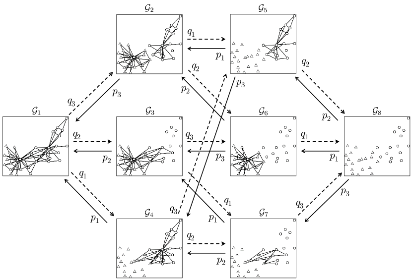
Figure 2: Transition diagram of the Markovian Karate Club Network

Using Proposition 1, we first illustrate how the time-variability of the Markovian Karate Network affects the behavior of epidemic threshold. We let the activation and deactivation rates of the edges be $p_{1}=p_{2}=0.1$, $q_{1}=q_{2}=1$, $p_{3}=0.02$, and $q_{3}=5$. As for the HeNeSIS model, we vary the value of the recovery rate $\delta$, uniformly at random among nodes, from $0$ to $2$. For each value of $\delta$, we use a bisection search to find the supremum $\beta_{c}$ of the transmission rate $\beta$ that guarantees the exponentially fast extinction of the disease spread (i.e., $\lambda_{\max}(\mathscr{A}_{1})<0$). We show the obtained values of $\beta_{c}$ versus $\delta$ in Fig. 3. We can observe that, unlike in the case of static network, the threshold value $\beta_{c}$ in our case exhibits a nonlinear dependence on $\delta$.

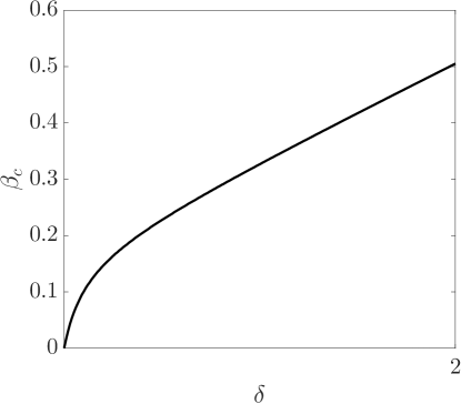
Figure 3: The epidemic threshold $\beta_{c}$ of the Markovian Karate Club Network versus the recover rate $\delta$.

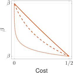
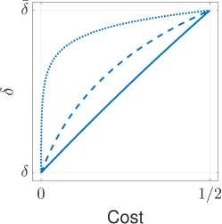
Figure 4: Left: Cost functions for transmission rates. Solid: $q=0.1$, dashed: $q=10$, dotted: $q=50$. Right: Cost function for recovery rates. $g$. Solid: $r=0.1$, dashed: $r=10$, dotted: $r=50$.

Table 1: Optimal investments for a) infection rates and b) recovery rates in the case of 1) the Markovian network and 2) time-aggregated network, respectively. Darker node colors represent heavier investments to vaccinate/antidote the node, while white nodes do not receive any investment.

	a) Infection rates	b) Recovery rates
1) Markovian 1) network
2) Time- 2) aggregated 2) network

We then move to the cost-optimal eradication of epidemic outbreaks over the Markovian Karate Network. Let us fix $\underaccent{\bar}{\delta}=p_{1}/2=0.05$ and $\bar{\beta}=\beta_{c}$, which are considered to be the ‘natural’ recovery and infection rates of the nodes. We then assume that a full dose of vaccinations and antidotes can improve these rates at most 20%, i.e., we let

$$\underaccent{\bar}{\beta}=({0.8})\bar{\beta},\quad\bar{\delta}=(1.2)\underaccent{\bar}{\delta}.$$

The cost functions for tuning the rates are set to be

$$f(\beta)=c_{1}+c_{2}/{\beta^{q}},\quad g(\delta)=c_{3}+c_{4}/{(\hat{\delta}-\delta)^{r}},$$ (9)

where $q$ and $r$ are positive parameters that allow us to tune the shape of the cost functions; $c_{1}$, $\dotsc$, $c_{4}$ are constants to normalize the cost functions in such a way that $f(\underaccent{\bar}{\beta})=1/2$, $f(\bar{\beta})=0$, $g(\underaccent{\bar}{\delta})=0$, and $g(\underaccent{\bar}{\delta})=1/2$. Notice that, with this choice of the normalization constants, we have $R=0$ if $(\beta_{i},\delta_{i})=(\bar{\beta},\underaccent{\bar}{\delta})$ for every node $i$ (i.e., all nodes keep their natural infection and transmission rates), while $R=n$ (full protection) if $(\beta_{i},\delta_{i})=(\underaccent{\bar}{\beta},\bar{\delta})$ for every $i$ (i.e., all nodes receive the full amount of vaccinations and antidotes). We show plots of the above cost functions for various values of $q$ and $r$ in Fig. 4, when $\hat{\delta}=2\bar{\delta}$. In our numerical simulation, we use the values $q=r=0.1$, in which case the cost functions becomes almost linear (solid lines in Fig. 4). Setting the available budget as $\bar{R}=n/2$, we solve the optimization problem in Theorem 2.1 and obtain the sub-optimal resource allocation over the Markovian Karate Network (illustrated in the first row of Table 1). We can observe that the nodes at the ‘boundaries’ of clusters do not receive much investments. This is reasonable because the first and second clusters are effectively disconnected (due to the low activation rate $p_{3}$ and the high deactivation rate $q_{3}$ of edges between clusters) and, therefore, we do not need to worry too much about the infections occurring across different clusters.

For the sake of comparison, we solve the same resource allocation problem for the original (static) Karate Club Network using the framework presented in Preciado2014 and obtain another allocation of vaccines and antidotes over the network (shown in the second row of Table 1). We can see that, in the latter allocation of resources, some of the nodes at the boundaries of the clusters receive a full investment, unlike in the Markovian case. This observation shows that, by taking into account the time-variability of temporal networks, we are able to distribute resources in a more efficient manner.

3 Edge-Independent Networks

Although the framework presented in the previous section can theoretically deal with epidemic outbreaks on temporal networks presenting the Markovian property, the framework is not necessarily applicable to some realistic temporal networks having a large number of graph configurations (i.e., when the number $L$ is large under the notation in Section 2.1). For example, in the example studied in Section 2.3, it would be more realistic to assume that the activations and deactivations of edges within a cluster or between clusters occur not simultaneously (as assumed in the example) but rather respectively (or, independently of each other). However, if we allow independent edge activations and deactivations for all the 78 edges in the network, we would end up obtaining a Markovian temporal network having $L=2^{78}>10^{23}$ possible graph configurations, which makes the optimization problem (8) computationally hard to solve.

The aim of this section is to present an optimization framework to contain epidemic outbreaks over temporal networks where edges are allowed to activate and deactivate independently of each other. We specifically focus on the HeNeSIS model evolving over aggregated-Markovian edge-independent (AMEI) temporal networks introduced in Ogura2015c . We present an efficient method for sub-optimally tuning the infection and recovery rates of the nodes in the network for containing epidemic outbreak in AMEI temporal networks. Unlike the optimization problem (8), the computational complexity for solving the optimization problem presented in this section does not grow with respect to the number $L$ of graph configurations. We also remark that another advantage of the AMEI temporal networks is its ability of modeling non-exponential, heavy-tail distributions of inter-event times found in several experimental studies Cattuto2010 ; Stehle2011 .

3.1 Model

We start by presenting the definition of aggregated-Markovian edge-independent (AMEI) temporal network model Ogura2015c . For simplicity in our exposition, we shall adopt a formulation slightly simpler than the original one in Ogura2015c .

Definition 1 (Ogura2015c ).

Consider a collection of stochastically independent Markov processes $h_{ij}$ ($1\leq i<j\leq n$) taking values in the integer set $\{1,\dotsc,M_{ij}\}$. We partition the integer set $M_{ij}$ into $\{1,\dotsc,M_{ij}\}=\mathscr{A}_{ij}\cup\mathscr{D}_{ij}$, where $\mathscr{A}_{ij}$ is called the active set and $\mathscr{D}_{ij}$ the inactive set. An aggregated-Markovian edge-independent (AMEI for short) temporal network is a random and undirected temporal network $\mathscr{G}(t)$ in which the edge $\{i,j\}$ is present at time $t$ if $h_{ij}(t)$ is in the active set $\mathscr{A}_{ij}$ and not present if $h_{ij}(t)$ is in the inactive set $\mathscr{D}_{ij}$ (see Fig. 5 for an illustration).

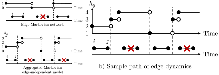
Figure 5: Example of the stochastic transitions of a particular edge in an AMEI model. Left: State-transition diagram of the Markov process $h_{ij}$ having the state space $\{1,2,3,4\}$ partitioned into the active set $\mathscr{A}_{ij}=\{1,2\}$ and the inactive set $\mathscr{D}_{ij}=\{3,4\}$. Right: a sample path of the time-evolution of the edge $\{i,j\}$.

A few remarks on the AMEI temporal networks are in order. First, the independence of the Markov processes $h_{ij}$ for all pairs of nodes ensures the independent dynamics of the connectivity of any node-pairs, unlike in the example presented in Section 2.3. Secondly, in the special case where $M_{ij}=2$, $\mathscr{A}_{ij}=\{1\}$, and $\mathscr{D}_{ij}=\{2\}$ for all $i$ and $j$, AMEI temporal networks reduce to the well-known model of temporal networks called the edge-Markovian model Clementi2008 . Thirdly, AMEI temporal networks in fact allow us to model a wider class of temporal networks. For example, in an edge-Markovian graph, the time it takes for an edge to switch from connected to disconnected (or vice versa) must follow an exponential distribution. In contrast, in an AMEI temporal network, we can design the active and inactive sets $\mathscr{A}_{ij},\mathscr{D}_{ij}$ as well as the Markov process $h_{ij}$ to fit any desired distribution for the contact durations with an arbitrary precision (Ogura2015c, , Example 1). Finally, since all the processes $h_{ij}$ are Markovian, the dynamics of an AMEI temporal network can be described by the collection $h=(h_{ij})_{i,j}$, which is again a Markov process.

3.2 Optimal Resource Allocation

In this section, we consider the same epidemiological problem as Problem 1:

Problem 2 (Nowzari2015b ).

Consider a HeNeSIS model over an AMEI temporal network. Given a budget $\bar{R}>0$, tune the infection and recovery rates $\beta_{i}$ and $\delta_{i}$ in the network in such a way that the exponential decay rate of the infection probabilities is minimized while satisfying the budget constraint $R\leq\bar{R}$ and the box constraints in (7).

We notice that, although Problem 2 is a particular case of Problem 1 for general Markovian temporal networks since an AMEI temporal network is Markovian, we cannot necessarily apply the optimization framework presented in Theorem 2.1 to the current case. Notice that an AMEI temporal network allows a total of $2^{m}$ graph configurations, where $m=2^{n(n-1)/2}$ is the number of the undirected edges that can exist in the network. This implies that the dimension of the vector-valued decision variable $v$ in the optimization problem (8), $nL=n2^{m}$, grows exponentially fast with respect to $n$, making it very hard to efficiently solve the optimization problem (8) even for small-scale networks. We further emphasize that this difficulty cannot be relaxed as long as we rely on the estimate on the decay rate of infection probabilities presented in Proposition 1, because the estimate already relies on a matrix of dimensions $(nL)\times(nL)$. This observation motivates us to derive an alternative, computationally efficient method for estimating the decay rate of infection probabilities. In this direction, using tools from random matrix theory, we are able to derive an alternative, tractable extinction condition for spreading processes over AMEI temporal networks Ogura2015c :

Proposition 2 ((Ogura2015c, , Theorem 3.4)).

For positive constants $b$ and $d$, define the decreasing function $\kappa(s)=n\exp(s/b)[(bs+d)/d]^{-(bs+d)/b^{2}}$ for $s\geq 0$. Let us consider the HeNeSIS spreading process over an AMEI temporal network. Define the $n\times n$ matrix $\bar{A}=[\bar{a}_{ij}]_{i,j}$ by

$$\bar{a}_{ij}=\lim_{t\to\infty}\Pr(a_{ij}(t)=1).$$ (10)

Let $\Delta=\max_{1\leq i\leq n}\sum_{j=1}^{n}\left(\beta_{i}\beta_{j}\bar{A}_{ij}(1-\bar{A}_{ij})\right)$ and $c=\eta(B(\operatorname{sgn}\bar{A})-D)-\kappa_{\beta_{\max},\Delta}^{-1}\!(1)$, where $\operatorname{sgn}(\cdot)$ denotes the entry-wise application of the sign function and $\beta_{\max}=\max_{1\leq i\leq n}\beta_{i}$. If

$$\lambda_{\max}(\mathscr{A}_{2})<\tau,$$ (11)

where

$$\mathscr{A}_{2}=B\bar{A}-D$$

and

$$\tau=\max_{s\in(\kappa_{\beta_{\max},\Delta}^{-1}\!(1),\underaccent{\bar}{\delta}+(\lvert c\rvert-c)/2]}\left(-\frac{s+c\kappa_{\beta_{\max},\Delta}(s)}{1-\kappa_{\beta_{\max},\Delta}(s)}\right),$$

then the infection probabilities converge to zero exponentially fast, almost surely.

The extinction condition (11) is comparable with the condition in (3) for static networks. Roughly speaking, we can understand $\bar{A}$ defined in (10) as the adjacency matrix of a weighted static network $\bar{\mathscr{G}}$ ‘representing’ the original AMEI temporal network, while $\tau$ can be regarded as a safety margin we have to take at the cost of utilizing this simplification. We further notice that the static network $\bar{\mathscr{G}}$ arises by taking a long-time limit of the original AMEI temporal network Ogura2015c . We finally remark that it is possible to upper-bound the decay rate of the convergence of infection probabilities using the maximum real eigenvalue of $\mathscr{A}_{2}$ (for details, see Ogura2015c ).

Proposition 2 gives us the following two alternative options to solve Problem 2 for a given HeNeSIS spreading process over an AMEI temporal network: 1) to increase $\tau$ or 2) to decrease $\lambda_{\max}(\mathscr{A}_{2})$. Among these two options, the former is not realistic because $\tau$ has a complicated expression and depends on relevant parameters in a highly complex manner. On the other hand, the maximum real eigenvalue $\lambda_{\max}(\mathscr{A}_{2})$ is easily tractable by the framework used in Section 2.2. This consideration leads us to the following sub-optimal solution to Problem 2:

Theorem 3.1 ((Ogura2015a, , Section VI)).

Assume that the cost function $f$ is a posynomial and, also, there exists $\hat{\delta}>\bar{\delta}$ such that the function $\tilde{g}(\tilde{\delta})=g(\hat{\delta}-\tilde{\delta})$ is a posynomial in $\tilde{\delta}$. Then, the infection and recovery rates that sub-optimally solve Problem 2 are given by $\{\beta_{i}^{\star}\}_{i=1}^{n}$ and $\{\hat{\delta}-\tilde{\delta}_{i}^{\star}\}_{i=1}^{n}$, where the starred variables solve the optimization problem

$$\operatorname*{\text{minimize}}_{\beta_{i},\,\tilde{\delta}_{i},\,v>0,\,\lambda>0} 1/\lambda$$

subject to $$\mathscr{A}_{2}v\leq-\lambda v,$$

$${\sum_{i=1}^{n}(f(\beta_{i})+\tilde{g}(\tilde{\delta}_{i}))}\leq\bar{R},$$

$${\underaccent{\bar}{\beta}}\leq\beta_{i}\leq\bar{\beta},$$

$$\hat{\delta}-\bar{\delta}\leq\tilde{\delta}_{i}\leq\hat{\delta}-\underaccent{\bar}{\delta}.$$

Moreover, this optimization problem can be equivalently converted to a geometric program.

3.3 Numerical simulation

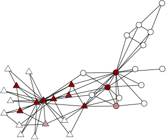
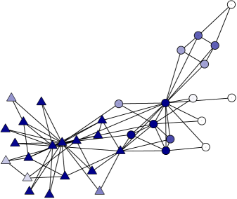
Figure 6: Optimal resource allocation for the AMEI Karate Club Network. Left: costs for transmission rates. Right: costs for recovery rates. Darker colors represent heavier investments, while white nodes do not receive any investment.

In this subsection, we illustrate the optimization framework for the optimal resource allocation over AMEI temporal networks presented in Theorem 3.1. For simplicity in the presentation, and to be consistent with the Markovian case in the previous section, we focus on the case where the edge-dynamics $h_{ij}$ of any edge $\{i,j\}$ is a two-state Markov process taking values in the set $\{1,2\}$ with the active set $\mathscr{A}_{ij}=\{1\}$ and the inactive set $\mathscr{D}_{ij}=\{2\}$ (although the following analysis can be applied to the general non-Markovian case where the edge-dynamics is explained by multi-state Markov processes $h_{ij}$). In this subsection, we consider the HeNeSIS spreading model over an AMEI temporal network based on the static Karate Network. Recall that, in the Markovian Karate Network, the activations and deactivations of edges within a cluster (or between clusters) must occur simultaneously. In this numerical simulation, we assume that these activations and deactivations occur independently of other edges. We specifically construct our AMEI temporal network as follows. For an edge $\{i,j\}$ between the nodes belonging to the first (or second) cluster, we let $h_{ij}$ be the two-state Markov process whose activation and deactivation rates are given by $p_{1}$ and $q_{1}$ ($p_{2}$ and $q_{2}$, respectively). Also, we let the activation and deactivation rates of edges between different clusters to be $p_{3}$ and $q_{3}$. Finally, for a pair $\{i,j\}$ of nodes not connected in the static Karate Club Network, we let their activation and deactivation rates to be $0$ and $1$, respectively. This choice guarantees that edges not present in the static network do not appear in our AMEI Karate network.

Using the cost function in (9), as well as the box constraints and budget $\bar{R}=n/2$ used in Section 2.3, we sub-optimally solve Problem 2 by using Theorem 3.1. The obtained resource distribution is illustrated in Fig. 6. As for the infection rates, we observe that nodes at the ‘boundaries’ of the clusters receive small investments, as already observed in the Markovian case. On the other hand, we cannot clearly observe this phenomena for recovery rates. We finally notice that the resulting investment heavily leans towards increasing recovery rates, not decreasing infection rates.

4 Adaptive Networks

In the case of epidemic outbreaks, it is commonly observed that the connectivity of human networks is severely influenced by the progress of the disease spread. This phenomenon, called social distancing Bell2006 ; Funk2010 , is known to help societies cope with epidemic outbreaks. A key feature of temporal networks of this type is their dependence on the nodal infection states. However, this structural dependence (or adaptation) cannot be well captured by the Markovian temporal networks because, in those networks, the dynamics of the network structure is assumed to be independent of the nodal states. In this direction, the aim of the current section is to present the so-called Adaptive SIS model Guo2013 ; Ogura2015i , which is able to replicate adaptation mechanisms found in realistic networks. We first present a tight extinction condition of epidemic outbreaks evolving in the ASIS model. Based on this extinction condition, we then illustrate how one can tune the adaptation rates of networks to eradicate epidemic outbreaks over the ASIS model.

4.1 Model

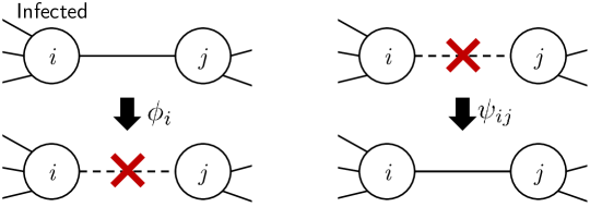
Figure 7: Adaptation mechanisms in the Adaptive SIS model.

In this section, we first describe the heterogeneous Adaptive SIS (ASIS) model Ogura2015i . As in the HeNeSIS model over Markovian temporal networks (studied in the previous two sections), the ASIS model consists of the following two components: the $\{0,1\}$-valued infectious, nodal states $x_{i}(t)$ and a temporal network $\mathscr{G}(t)$. While the nodal states in the ASIS model have the same transition probabilities as in (5), the transition probabilities of the network $\mathscr{G}(t)$ in the ASIS model are quite different from Markovian temporal networks because the probabilities depend on the states of the nodes, as described below. Let $\mathscr{G}(0)=(\mathscr{V},\mathscr{E}(0))$ be an initial connected contact graph with adjacency matrix $A(0)=[a_{ij}(0)]_{i,j}$. Then, edges in the initial graph $\mathscr{G}(0)$ appear and disappear over time according to the following transition probabilities:

$$\Pr(a_{ij}(t+h)=0\mid a_{ij}(t)=1) =\phi_{i}x_{i}(t)h+\phi_{j}x_{j}(t)h+o(h),$$ (12)

$$\Pr(a_{ij}(t+h)=1\mid a_{ij}(t)=0) =a_{ij}(0)\psi_{ij}h+o(h),$$ (13)

where the parameters $\phi_{i}>0$ and $\psi_{ij}=\psi_{ji}>0$ are called the cutting and reconnecting rates, respectively. Notice that the transition rate in (12) depends on the nodal states $x_{i}$ and $x_{j}$, inducing an adaptation mechanism of the network structure to the state of the epidemics. The transition probability in (12) can be interpreted as a protection mechanism in which edge $\{i,j\}$ is stochastically removed from the network if either node $i$ or $j$ is infected. More specifically, because of the first summand (respectively, the second summand) in (12), whenever node $i$ (respectively, node $j$) is infected, edge $\{i,j\}$ is removed from the network according to a Poisson process with rate $\phi_{i}$ (respectively, rate $\phi_{j}$). On the other hand, the transition probability in (13) describes a mechanism for which a ‘cut’ edge $\{i,j\}$ is ‘reconnected’ into the network according to a Poisson process with rate $\psi_{ij}$ (see Fig. 7). Notice that we include the term $a_{ij}(0)$ in (13) to guarantee that only edges present in the initial contact graph $\mathscr{G}(0)$ can be added later on by the reconnecting process. In other words, we constrain the set of edges in the adaptive network to be a part of the arbitrary contact graph $\mathscr{G}(0)$.

4.2 Optimal Resource Allocation

In this section, we consider the situation in which we can tune the values of the cutting rates in the network by incurring a cost. In particular, we can tune the value of the cutting rate of node $i$ to $\phi_{i}$ by incurring a cost of $h(\phi_{i})$. The total tuning cost is therefore given by $R=\sum_{i=1}^{n}h(\phi_{i})$. In this setup, we can state the optimal resource allocation problem, as follows:

Problem 3.

Consider a heterogeneous ASIS model. Given a budget $\bar{R}$, tune the cutting rates $\phi_{i}$ in the network in such a way that the exponential decay rate of the infection probabilities is minimized while satisfying the budget constraint $R\leq\bar{R}$ and the box-constraint $0<\underaccent{\bar}{\phi}\leq\phi_{i}\leq\bar{\phi}$.

In order to solve this problem, we shall follow the same path as we did in the previous sections: we first find an analytical estimate of the decay rate of the infection probabilities in the ASIS model. For this purpose, we first represent the ASIS model by a set of stochastic differential equations described below (see Ogura2015i for details). For $\gamma>0$, let $N_{\gamma}$ denote a Poisson counter with rate $\gamma$ Feller1956vol1 . Then, from the two equations in (5), the evolution of the nodal states can be exactly described by the following stochastic differential equation:

$$dx_{i}=-x_{i}\,dN_{\delta_{i}}+(1-x_{i})\sum_{j\in\mathscr{N}_{i}(0)}a_{ij}x_{j}\,dN_{\beta_{i}},$$ (14)

for all nodes $i$. Similarly, from (12) and (13), the evolution of the edges can be exactly described by

$$da_{ij}=-a_{ij}(x_{i}\,dN_{\phi_{i}}+x_{j}\,dN_{\phi_{j}})+(1-a_{ij})\,dN_{\psi_{ij}},$$ (15)

for all $\{i,j\}\in\mathscr{E}(0)$. Then, by (14), the expectation $E[x_{i}]$ obeys the differential equation $(d/dt)E[x_{i}]=-\delta_{i}E[x_{i}]+\beta_{i}\sum_{{k\in\mathscr{N}_{i}(0)}}E[(1-x_{i})a_{ik}x_{k}]$. Let $p_{i}(t)=E[x_{i}(t)]$ and $q_{ij}(t)=E[a_{ij}(t)x_{i}(t)]$. Then, it follows that

$$\frac{dp_{i}}{dt}=-\delta_{i}p_{i}+\beta_{i}\sum_{{j\in\mathscr{N}_{i}(0)}}q_{ji}-f_{i},$$ (16)

where $f_{i}=\beta_{i}\sum_{k\in\mathscr{N}_{i}(0)}E[x_{i}x_{k}a_{ik}]$ contains positive higher-order terms. Similarly, from (14) and (15), the Ito formula for stochastic differential equations (see, e.g., Hanson2007 ) shows that

$$\frac{dq_{ij}}{dt}= -\phi_{i}p_{ij}+\psi_{ij}(p_{i}-q_{ij})-\delta_{i}q_{ij}+\beta_{i}\ \sum_{{k\in\mathscr{N}_{i}(0)}}\ q_{ki}-g_{ij},$$ (17)

where $g_{ij}=\phi_{j}E[x_{i}x_{j}a_{ij}]+\beta_{i}\sum_{{k\in\mathscr{N}_{i}(0)}}E[x_{i}x_{k}a_{ik}+(1-a_{ij})a_{ik}x_{k}]$ contains positive higher-order terms. We remark that the differential equations (16) and (17) exactly describe the joint evolution of the spreading process and the network structure without relying on mean-field approximations.

Based on the above derivation, we are able to prove the following proposition:

Proposition 3 (Ogura2015i ).

Let $T_{i}$ be the unique row-vector satisfying $T_{i}q=\sum_{{k\in\mathscr{N}_{i}(0)}}q_{ki}$. Define the matrices

$$\begin{gathered}B_{1}=\operatorname*{col}_{1\leq i\leq n}(\beta_{i}T_{i}),\quad B_{2}=\operatorname*{col}_{1\leq i\leq n}(\beta_{i}\mathbbold{1}_{d_{i}}\otimes T_{i}),\quad D_{1}=\bigoplus_{i=1}^{n}\delta_{i},\quad D_{2}=\bigoplus_{i=1}^{n}(\delta_{i}I_{d_{i}}),\\ \Phi=\bigoplus_{i=1}^{n}(\phi_{i}I_{d_{j}}),\quad\Psi_{1}=\bigoplus_{i=1}^{n}(\operatorname*{col}_{j\in{\mathscr{N}}_{i}(0)}\psi_{ij}),\quad\Psi_{2}=\bigoplus_{i=1}^{n}\bigoplus_{j\in\mathscr{N}_{i}(0)}\psi_{ij},\end{gathered}$$

where $d_{i}$ denotes the degree of node $i$ in the initial graph $\mathscr{G}(0)$, $\otimes$ denotes the Kronecker product Brewer1978 of matrices, and $\mathbbold{1}_{n}$ denotes the all-one vector of length $n$. If the matrix

$$\mathscr{A}_{3}=\begin{bmatrix}-D_{1}&B_{1}\\ \Psi_{1}&B_{2}-D_{2}-\Phi-\Psi_{2}\end{bmatrix}$$

satisfies

$$\lambda_{\max}(\mathscr{A}_{3})<0,$$ (18)

then the infection probabilities in the heterogeneous ASIS model converge to zero exponentially fast with an exponential decay rate $|\lambda_{\max}(\mathscr{A}_{3})|$.

We remark that, in the homogeneous case, where all the nodes share the same infection rate $\beta>0$ and recovery rate $\delta>0$, and all the edges share the same cutting rate $\phi>0$ and reconnecting rate $\psi>0$, the condition in (18) reduces Ogura2015i to the following simple inequality:

$$\frac{\beta}{\delta}<\frac{1+\omega}{\lambda_{\max}(A(0))},$$ (19)

where $\omega={\phi}/{(\delta+\psi)}$ is called the effective cutting rate. The proof of this reduction can be found in (Ogura2015i, , Appendix B). We remark that, in the special case when the network does not adapt to the prevalence of infection, i.e., when $\phi=0$, we have that $\omega=0$ and, therefore, the condition in (19) is identical to the extinction condition (4) corresponding to the homogeneous networked SIS model over a static network VanMieghem2009a .

Now, based on Proposition 3, one can yield the following solution to Problem 3 based on geometric programs:

Theorem 4.1 ((Ogura2015i, , Section IV)).

Assume that there exists $\hat{\phi}>\bar{\phi}$ such that the function $\tilde{h}(\tilde{\phi})=h(\hat{\phi}-\tilde{\phi})$ is a posynomial in $\tilde{\phi}$. Then, the cutting rates that sub-optimally solve Problem 3 are given by $\{\hat{\phi}-\tilde{\phi}_{i}^{\star}\}_{i=1}^{n}$, where the starred variables solve the optimization problem:

$$\operatorname*{\text{minimize}}_{\tilde{\phi}_{i},\,v>0,\,\lambda>0} 1/\lambda$$

subject to $$\mathscr{A}_{3}v\leq-\lambda v,$$

$$\sum_{i=1}^{n}\tilde{h}(\tilde{\phi}_{i})\leq\bar{R},$$

$$\hat{\phi}-\bar{\phi}\leq\tilde{\phi}_{i}\leq\hat{\phi}-\underaccent{\bar}{\phi}.$$

Moreover, this optimization problem can be equivalently converted to a geometric program.

4.3 Numerical simulations

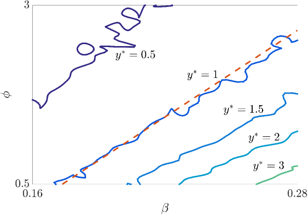
Figure 8: The meta-stable number of the infected nodes $y^{*}$ versus $\beta$ and $\phi$, with $\delta=1$ and $\psi=2$. The dashed straight lines show the analytically derived lower bound $(1+\omega)/\lambda_{\max}(A(0))=\beta$ on the epidemic threshold.

In this section, we illustrate the results presented in this section. Let the initial graph $\mathscr{G}(0)$ be the Karate Club Network. We first consider the homogeneous case, and fix the recovery rate and the reconnecting rate in the network to be $\delta=1$ and $\psi=2$ for all nodes in the graph, for the purpose of illustration. We then compute the meta-stable number $y^{*}$ of the infected nodes in the network for various values of $\beta$ and $\phi$ (for details of this simulation, see Ogura2015i ). The obtained metastable numbers are shown as a contour plot in Fig. 8. We see how the analytical threshold $\beta/\delta=(1+\omega)/\lambda_{\max}(A(0))$ from (19) (represented as a dashed straight line in Fig. 8) is in good accordance with the numerically found threshold $y^{*}=1$.

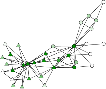
Figure 9: The distribution of the resource for tuning the cutting rates in the ASIS Karate Network

We then consider the optimal resource distribution problem stated in Problem 3. In this simulation, we use the cost function $h(\phi)=c_{5}+c_{6}/(\hat{\phi}-\phi)^{s}$ similar to the one used in (9), where $s$ is a positive parameter for tuning the shape of the cost function, $\hat{\phi}$ is a constant larger than $\bar{\phi}$, and $c_{5}$ and $c_{6}$ are constants such that $h(\underaccent{\bar}{\phi})=0$ and $h(\bar{\phi})=1$. We let $\underaccent{\bar}{\phi}=0.5$, $\bar{\phi}=1.5$, $\hat{\phi}=100\bar{\phi}$, and $s=1$, for which the resulting cost function resembles a linear function as in the case of Markovian temporal networks. Using these cost functions and the budget $\bar{R}=n/2$, we solve the optimization problem in Theorem 4.1 to find the sub-optimal distribution of resource over the network (illustrated in Fig. 9). Interestingly, unlike in the Markovian cases in Sections 2 and 3, we cannot clearly observe the phenomenon where nodes at the boundaries of the clusters receive relatively less investments.

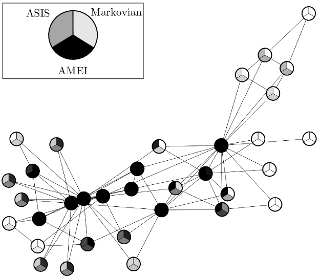
Figure 10: Optimal spending on nodes. In each circle (node), the upper-right, lower, and upper-left colors indicate the investments according to the Markovian, AMEI, and ASIS formulations, respectively.

Finally, in Fig. 10, we summarize the amount of optimal resource distributions obtained for the Markovian, AMEI, and ASIS Karate Networks. We see that, although the three allocations share a certain tendency such as concentration of resource on high-degree nodes, they are not necessarily qualitatively equal. This observation confirms the necessity of appropriately incorporating the characteristics of temporal/adaptive networks into our mechanism of resource distributions.

5 Conclusion

In this chapter, we have given an overview of recent progress on the problem of containing epidemic outbreaks taking place in temporal and adaptive complex networks. Specifically, we have presented analytical frameworks for finding the optimal distribution of resources over Markovian temporal networks, aggregated-Markovian edge-independent temporal networks, and in the Adaptive SIS model. For each of the cases, we have seen that the optimal resource distribution problems can be reduced to an efficiently solvable class of convex optimizations called geometric programs. We have illustrated the results with several numerical simulations based on the well-studied Zachary Karate Club Network.

- (1) Ahn, H.J., Hassibi, B.: Global dynamics of epidemic spread over complex networks. In: 52nd IEEE Conference on Decision and Control, pp. 4579–4585 (2013).
- (2) Antoniades, D., Dovrolis, C.: Co-evolutionary dynamics in social networks: a case study of Twitter. Computational Social Networks 2(1), 14 (2015).
- (3) Barrat, A., Barthelemy, M., Vespignani, A.: Dynamical Processes on Complex Networks. Cambridge University Press (2008)
- (4) Bell, D., Nicoll, A., Fukuda, K., Horby, P., Monto, A., Hayden, F., Wylks, C., Sanders, L., Van Tam, J.: Nonpharmaceutical interventions for pandemic influenza, national and community measures. Emerging Infectious Diseases 12(1), 88–94 (2006).
- (5) Borgs, C., Chayes, J., Ganesh, A., and Saberi, A.: How to distribute antidote to control epidemics. Random Structures and Algorithms 37(2), 204–222 (2010).
- (6) Boyd, S., Kim, S.J., Vandenberghe, L., Hassibi, A.: A tutorial on geometric programming. Optimization and Engineering 8(1), 67–127 (2007).
- (7) Boyd, S., Vandenberghe, L.: Convex Optimization. Cambridge University Press (2004)
- (8) Brewer, J.: Kronecker products and matrix calculus in system theory. IEEE Transactions on Circuits and Systems 25(9), 772–781 (1978).
- (9) Cattuto, C., van den Broeck, W., Barrat, A., Colizza, V., Pinton, J.F., Vespignani, A.: Dynamics of person-to-person interactions from distributed RFID sensor networks. PLoS ONE 5(7) (2010)
- (10) Chen, X., and Preciado, V.M.: Optimal coinfection control of competitive epidemics in multi-layer networks. In: Proceedings IEEE Conference on Decision and Control, pp. 6209–6214 (2014).
- (11) Chung, F., Horn, P., and Tsiatas, A.: Distributing antidote using pagerank vectors. Internet Mathematics 6(2), 237–254 (2009).
- (12) Clementi, A.E., Macci, C., Monti, A., Pasquale, F., Silvestri, R.: Flooding time in edge-Markovian dynamic graphs. In: 27th ACM Symposium on Principles of Distributed Computing, pp. 213–222 (2008).
- (13) Cohen, R., Havlin, S., and Ben-Avraham, D.: Efficient immunization strategies for computer networks and populations. Physical Review Letters 91(24), 247901 (2003).
- (14) Drakopoulos, K., Ozdaglar, A., and Tsitsiklis, J.N.: An efficient curing policy for epidemics on graphs. IEEE Transactions on Network Science and Engineering, 1(2), 67–75 (2014).
- (15) Feller, W.: An Introduction to Probability Theory and Its Applications. John Wiley & Sons (1956)
- (16) Funk, S., Salathé, M., Jansen, V.A.A.: Modelling the influence of human behaviour on the spread of infectious diseases: a review. Journal of the Royal Society, Interface / the Royal Society 7, 1247–1256 (2010).
- (17) Ganesh, A., Massoulie, L., and Towsley, D.: The effect of network topology on the spread of epidemics. In: Proceedings INFOCOM, pp. 1455–1466 (2005)
- (18) Gross, T., Blasius, B.: Adaptive coevolutionary networks: a review. Journal of the Royal Society, Interface / the Royal Society 5(20), 259–271 (2008).
- (19) Guo, D., Trajanovski, S., van de Bovenkamp, R., Wang, H., Van Mieghem, P.: Epidemic threshold and topological structure of susceptible-infectious-susceptible epidemics in adaptive networks. Physical Review E 88, 042802 (2013).
- (20) Hanson, F.B.: Applied Stochastic Processes and Control for Jump-Diffusions: Modeling, Analysis and Computation. Society for Industrial and Applied Mathematics (2007)
- (21) Holme, P.: Modern temporal network theory: a colloquium. The European Physical Journal B 88(9), 234 (2015).
- (22) Holme, P., Liljeros, F.: Birth and death of links control disease spreading in empirical contact networks. Scientific Reports 4, 4999 (2014).
- (23) Horn, R., Johnson, C.: Matrix Analysis. Cambridge University Press (1990)
- (24) Karsai, M., Kivelä, M., Pan, R.K., Kaski, K., Kertész, J., Barabasi, A.L., Saramäki, J.: Small but slow world: How network topology and burstiness slow down spreading. Physical Review E 83(2), 025102 (2011).
- (25) Karsai, M., Perra, N., Vespignani, A.: Time varying networks and the weakness of strong ties. Scientific Reports 4, 4001 (2014).
- (26) Khanafer, A., and Basar, T.: An optimal control problem over infected networks. In: Proc. International Conference on Control, Dynamic Systems, and Robotics, pp. 1–6 (2014).
- (27) Khouzani, M. H. R., Sarkar, S., and Altman, E.: Optimal control of epidemic evolution. In: Proceedings IEEE INFOCOM, pp. 1683–1691 (2011).
- (28) Lajmanovich, A., Yorke, J.A.: A deterministic model for gonorrhea in a nonhomogeneous population. Mathematical Biosciences 28(1976), 221–236 (1976).
- (29) Liu, S., Perra, N., Karsai, M., Vespignani, A.: Controlling contagion processes in activity driven networks. Physical Review Letters 112(11), 118702 (2014). URL http://link.aps.org/doi/10.1103/PhysRevLett.112.118702
- (30) Nowzari, C., Preciado, V.M., and Pappas, G.J.: Stability analysis of generalized epidemic models over directed networks. In: Proceedings IEEE Conference on Decision and Control, pp. 6197–6202 (2014).
- (31) Nowzari, C., Ogura, M., Preciado, V.M., and Pappas, G.J.: A general class of spreading processes with non-Markovian dynamics. In: Proceedings IEEE Conference on Decision and Control, pp. 5073–5078 (2015).
- (32) Masuda, N., Holme, P.: Predicting and controlling infectious disease epidemics using temporal networks. F1000prime reports 5:6(March) (2013).
- (33) Masuda, N., Klemm, K., Eguíluz, V.M.: Temporal networks: Slowing down diffusion by long lasting interactions. Physical Review Letters 111(18), 1–5 (2013).
- (34) Newman, M., Barabási, A.L., Watts, D.J.: The Structure and Dynamics of Networks. Princeton University Press (2006)
- (35) Nowzari, C., Ogura, M., Preciado, V.M., Pappas, G.J.: Optimal resource allocation for containing epidemics on time-varying networks. In: 49th Asilomar Conference on Signals, Systems and Computers, pp. 1333–1337 (2015).
- (36) Nowzari, C., Preciado, V.M., Pappas, G.J.: Analysis and control of epidemics: A survey of spreading processes on complex networks. IEEE Control Systems 36(1), 26–46 (2016).
- (37) Ogura, M., Martin, C.F.: Stability analysis of positive semi-Markovian jump linear systems with state resets. SIAM Journal on Control and Optimization 52, 1809–1831 (2014).
- (38) Ogura, M., Preciado, V.M.: Optimal design of switched networks of positive linear systems via geometric programming. IEEE Transactions on Control of Network Systems (accepted) (2015).
- (39) Ogura, M., Preciado, V.M.: Epidemic processes over adaptive state-dependent networks. Physical Review E 93, 062316 (2016).
- (40) Ogura, M., Preciado, V.M.: Optimal design of networks of positive linear systems under stochastic uncertainty. In: 2016 American Control Conference, pp. 2930–2935 (2016).
- (41) Ogura, M., Preciado, V.M.: Stability of spreading processes over time-varying large-scale networks. IEEE Transactions on Network Science and Engineering 3(1), 44–57 (2016).
- (42) Pastor-Satorras, R., Castellano, C., Van Mieghem, P., Vespignani, A.: Epidemic processes in complex networks. Reviews of Modern Physics 87(3), 925–979 (2015).
- (43) Perra, N., Gonçalves, B., Pastor-Satorras, R., Vespignani, A.: Activity driven modeling of time varying networks. Scientific Reports 2:469 (2012).
- (44) Preciado, V.M., Zargham, M., Enyioha, C., Jadbabaie, A., and Pappas, G.J.: Optimal vaccine allocation to control epidemic outbreaks in arbitrary networks. In: Proceedings IEEE Conference on Decision and Control, pp. 7486–7491 (2013).
- (45) Preciado, V.M., and Zargham, M.: Traffic optimization to control epidemic outbreaks in metapopulation models. In: Global Conference on Signal and Information Processing, pp. 847–850 (2013).
- (46) Preciado, V.M., Sahneh, F.D., and Scoglio, C.: A convex framework for optimal investment on disease awareness in social networks. In: Global Conference on Signal and Information Processing, pp. 851–854 (2013).
- (47) Preciado, V. M., and Jadbabaie, A.: Spectral analysis of virus spreading in random geometric networks. In: Proceedings IEEE Conference on Decision and Control, pp. 4802–4807 (2009).
- (48) Preciado, V.M., Zargham, M., Enyioha, C., Jadbabaie, A., Pappas, G.J.: Optimal resource allocation for network protection against spreading processes. IEEE Transactions on Control of Network Systems 1(1), 99–108 (2014).
- (49) Ramirez-Llanos, E., and Martinez, S.: Distributed and robust fair resource allocation applied to virus spread minimization. In: Proceedings IEEE American Control Conference, pp. 1065–1070 (2015).
- (50) Rocha, L.E.C., Blondel, V.D.: Bursts of vertex activation and epidemics in evolving networks. PLoS computational biology 9(3), e1002974 (2013).
- (51) Rogers, T., Clifford-Brown, W., Mills, C., Galla, T.: Stochastic oscillations of adaptive networks: application to epidemic modelling. Journal of Statistical Mechanics: Theory and Experiment 2012(08), P08018 (2012).
- (52) Sahneh, F.D., and Scoglio, C.: Competitive epidemic spreading over arbitrary multilayer networks. Physical Review E 89, 062817 (2014).
- (53) Schaper, W., Scholz, D.: Factors regulating arteriogenesis. Arteriosclerosis, Thrombosis, and Vascular Biology 23(7), 1143–1151 (2003).
- (54) Schwarzkopf, Y., Rákos, A., Mukamel, D.: Epidemic spreading in evolving networks. Physical Review E 82(3), 036112 (2010).
- (55) Scirè, A., Tuval, I., Eguíluz, V.M.: Dynamic modeling of the electric transportation network. Europhysics Letters 71(2), 318–324 (2005).
- (56) Stehlé, J., Voirin, N., Barrat, A., Cattuto, C., Isella, L., Pinton, J.F., Quaggiotto, M., van den Broeck, W., Régis, C., Lina, B., Vanhems, P.: High-resolution measurements of face-to-face contact patterns in a primary school. PLoS ONE 6(8) (2011)
- (57) Szabó-Solticzky, A., Berthouze, L., Kiss, I.Z., Simon, P.L.: Oscillating epidemics in a dynamic network model: stochastic and mean-field analysis. Journal of Mathematical Biology 72(5), 1153–1176 (2016).
- (58) Taylor, M., Taylor, T.J., Kiss, I.Z.: Epidemic threshold and control in a dynamic network. Physical Review E 85(1), 016103 (2012).
- (59) Torres, J.A., Roy, S., and Wan, Y.: Sparse allocation of resources in dynamical networks with application to spread control. In: Proceedings IEEE American Control Conference, pp. 1873–1878 (2015).
- (60) Trajanovski, S., Hayel, Y., Altman, E., Wang, H., Van Mieghem, P.: Decentralized protection strategies against SIS epidemics in networks. IEEE Transactions on Control of Network Systems 2(4), 406–419 (2015).
- (61) Tunc, I., Shaw, L.B.: Effects of community structure on epidemic spread in an adaptive network. Physical Review E 90(2), 022801 (2014).
- (62) Valdez, L.D., Macri, P.A., Braunstein, L.A.: Intermittent social distancing strategy for epidemic control. Physical Review E 85, 036108 (2012).
- (63) Van Mieghem, P., Omic, J., Kooij, R.: Virus spread in networks. IEEE/ACM Transactions on Networking 17(1), 1–14 (2009).
- (64) Vazquez, A., Rácz, B., Lukács, A., Barabasi, A.L.: Impact of non-Poissonian activity patterns on spreading processes. Physical Review Letters 98(15), 158702 (2007).
- (65) Vestergaard, C.L., Génois, M., Barrat, A.: How memory generates heterogeneous dynamics in temporal networks. Physical Review E 90(4), 042805 (2014).
- (66) Volz, E., Meyers, L.A.: Epidemic thresholds in dynamic contact networks. Journal of the Royal Society, Interface / the Royal Society 6(32), 233–241 (2009).
- (67) Von Luxburg, U.: A tutorial on spectral clustering. Statistics and Computing 17(4), 395–416 (2007).
- (68) Wang, B., Cao, L., Suzuki, H., Aihara, K.: Epidemic spread in adaptive networks with multitype agents. Journal of Physics A: Mathematical and Theoretical 44(3), 035,101 (2011).
- (69) Watkins, N.J., Nowzari, C., Preciado, V.M., Pappas, G.J.: Optimal resource allocation for competitive spreading processes on bilayer networks. IEEE Transactions on Control of Network Systems (accepted) (2016).
- (70) Wan, Y., Roy, S., and Saberi, A.: Designing spatially heterogeneous strategies for control of virus spread. IET Systems Biology, 2(4), 184–201 (2008).
- (71) Watkins, N.J., Nowzari, C., Preciado, V.M., and Pappas, G.J.: Optimal resource allocation for competing epidemics over arbitrary networks. In: Proceedings IEEE American Control Conference, pp. 1381–1386 (2015).
- (72) Watts, D.J., Strogatz, S.H.: Collective dynamics of ’small-world’ networks. Nature 393(6684), 440–442 (1998).
- (73) Zachary, W.W.: An information flow model for conflict and fission in small groups. Journal of Anthropological Research 33(4), 452–473 (1977).