Neutron Moderation Theory Taking into Accout the Thermal Motion of Moderating Medium Nuclei

Abstract

In this paper we present the analytical expression for the neutron scattering law for an isotropic source of neutrons, obtained within the framework of the gas model with the temperature of the moderating medium as a parameter. The obtained scattering law is based on the solution of the kinematic problem of elastic scattering of neutrons on nuclei in the $L$-system in the general case. I.e. both the neutron and the nucleus possess the arbitrary velocity vectors in the $L$-system. For the new scattering law the flux densities and neutron moderation spectra depending on the temperature are obtained for the reactor fissile medium. The expressions for the moderating neutrons spectra allow reinterpreting the physical nature of the underlying processes in the thermal region.

Department of Theoretical and Experimental Nuclear Physics,
Odessa National Polytechnic University, Odessa, Ukraine

1 Introduction

An important part of the theory of neutron cycle in nuclear reactors is the theory of neutron moderation [1, 2, 3, 4, 5, 6, 7]. A neutron moderation theory traditionally used in contemporary nuclear reactor physics was developed in the framework of the gas model. This model neglects the interaction between neutrons and the nuclei of moderating medium, although some unfinished attempts were made to include the interaction between the nuclei of the moderating medium, e.g. in [2, 3]. This traditional theory of neutron moderation is based on the neutron scattering law which defines the energy distribution of the elastically scattered neutrons in the laboratory coordinate system ($L$-system) (see the neutron scattering law e.g. in [4, 5, 6]). The neutron scattering law, in its turn, is based on the solution of a kinematic problem of neutrons elastic scattering on the moderator nuclei[1, 2, 3, 4, 5, 6]. It should be noted however that we use the term ”scattering law” instead of the ”elastic scattering law”, because this solution is generalized for all kinds of scattering reactions (elastic and inelastic) during the formulation of the moderating neutrons balance equation. For example, as it is known from the neutron moderation theory, the moderating neutrons flux density is found as a solution of the balance equation for the moderating neutrons, and depends on the macroscopic scattering cross-section $\Sigma_{s}$ in case of the moderator without neutron absorption, and on the total macroscopic cross-section $\Sigma_{t}$ in case of the moderator with neutron absorption (see [1, 2, 3, 4, 5, 6] and sections 4-7 below). Let us remind that $\Sigma_{s}=\Sigma_{el}+\Sigma_{in}$ where $\Sigma_{el}=\Sigma_{p}+\Sigma_{rs}$ is the macroscopic elastic scattering cross-section, $\Sigma_{p}$ is the macroscopic potential scattering cross-section, $\Sigma_{rs}$ is the macroscopic resonance scattering cross-section, $\Sigma_{in}$ is the macroscopic inelastic scattering cross-section, and $\Sigma_{t}=\Sigma_{s}+\Sigma_{a}$, where $\Sigma_{a}$ is the macroscopic absorption cross-section for the moderating medium (e.g. [6]).

The kinematic problem of an elastic neutron scattering on a nucleus in the $L$-system is a two-particle kinematic problem and may be solved exactly. Still, a neat and compact analytical solution of such problem may be obtained only in the case of the nucleus resting in the $L$-system before scattering. In the general case, when both the neutron and the nucleus have arbitrary velocity vectors in the $L$-system before scattering, the solution of this problem is a set of cumbersome expressions. This is because of the fact that an intermediate solution including the cosines of the angles between the nucleus and neutron velocity vectors is located in the C-system, and is rather lengthy by itself. The final solution of the problem in the $L$-system requires a transformation of the cosines from the C-system to $L$-system. And this requires several more relations transforming the unit vectors from the C-system to the $L$-system. Therefore, reduction of the solution to a single analytical expression makes no sense in this case. However, in this case it is possible to build a computational algorithm to obtain the solution via computer calculation. This approach is implemented in modern Monte Carlo codes, e.g. MCNP4, GEANT4 and others, which let one calculate the moderating neutron spectrum even for the moderators with absorption. It should be noted that these Monte Carlo codes are used for the majority of today’s practical calculations involving the neutron spectra.

Still, the traditional theory of neutron moderation is based on the above mentioned analytical solution obtained for the case of the nucleus resting in the $L$-system before scattering. I.e. the traditional theory neglects the heat motion of the moderator nuclei, which is acceptable if the neutron energies are much higher than the thermal motion energy of the nuclei. As a consequence, the neutron scattering law and the following analytical expressions for the Fermi spectrum of the moderating neutrons do not contain the temperature of the moderating medium. In order to cover this significant gap in the theory, the only thing suggested until today was to complement the Fermi spectrum of the moderating neutrons with the Maxwell-type spectrum in the thermal energy range artificially (in the sense that this was not obtained strictly from the scattering law). Moreover, in order to form the Maxwell spectrum, it is necessary to recalculate the temperature of the moderating medium $T$ into the temperature of the neutron gas $T_{n}$ using the formula $T_{n}=T\left[1+1.8\frac{\Sigma_{a}(kT)}{\xi\Sigma_{s}}\right]$ (where $\Sigma_{a}(kT)$ is the macroscopic absorption cross-section for moderating medium and the neutrons of the energy $kT$, $\xi\Sigma_{s}$ is the moderating power of the moderator for the 1 eV neutrons). According to [1], this formula was obtained as a numerical approximation of the experimental spectra of several different types of nuclear reactors available at that time, and is still widely used in the reactor physics, e.g. [5, 6, 7, 8, 9, 10, 11, 12, 13, 14]. Let us also note that the multiplier before the second term in brackets is often chosen by the developers depending on the reactor type, e.g. [5, 9].

Because of the fission accompanied by the large energy release, the emission of neutrons and other particles, the nuclide composition change, the heat transfer, the radiation-induced defects dynamics (leading to the geometry change up to the complete destruction), reactor fissile medium is in the state of thermodynamic non-equilibrium. The same is true for any fissile medium with active chain reactions in it. I.e. the reactor fissile medium with the fission processes is an open physical system in the non-equilibrium thermodynamic state. Such system may be described within the framework of the non-linear non-equilibrium thermodynamics of the open physical systems. Such systems may include the non-equilibrium stationary states, which meet the Prigogine criterion – the minimum of the entropy production (e.g. [15, 16, 17]). The realization and type of such stationary mode are known to depend both on the internal parameters of the system (internal entropy) and on the boundary conditions (boundary entropy flow). For example, the realization of the stationary state in a non-equilibrium system (hereinafter referred to as stationary non-equilibrium state) requires the constant boundary conditions (see e.g. [16]).

In our model of the neutron moderation in the fissile medium the following simplifications are taken. Two thermodynamic subsystems are singled out from the fissile medium – the moderating neutrons subsystem and the moderator nuclei subsystem. The subsystems are open physical systems interacting with each other. Thus, according to the stated above, both of these systems are in the non-equilibrium state. However, in our case we assume the moderator nuclei subsystem to be near its equilibrium state because of its inertia relative to perturbations and negligible influence of the neutron subsystem. This allows us to introduce a temperature of the moderator medium. The neutron subsystem remains non-equilibrium in our model, and the temperature of this subsystem is not introduced. Let us emphasize that in order to construct the neutron spectrum, the traditional approach operates with the concept of temperature of the neutron gas, which indicates the usage of an additional simplification in it – the one that we refused to take. This fact, together with the aforementioned, led the authors to a conclusion that there was currently no robust and consistent theory of neutron moderation, and it was crucial to develop such a theory.

The absence of the moderation theory results in numerous difficulties related to the study of the reactor emergency modes, the development of the new generation nuclear reactors such as the traveling-wave reactors [18, 19], pulsed reactors, boosters, subcritical assemblies [20, 21, 22], and the investigation of the natural nuclear reactors such as georeactor [23].

Let us also note that the expressions for the moderating neutrons flux density obtained in the present paper, are the solutions of the equation describing the process of the neutron moderation in a stationary state, which may set within a non-equilibrium neutron system under certain conditions.

Thus, in the present paper, based on the solution of the kinematic problem of elastic neutron scattering on a nucleus in the $L$-system in general case (when both the neutron and the nucleus have arbitrary velocity vectors in the $L$-system before scattering) we derive the analytical expression for the neutron scattering law including the moderating medium temperature as a parameter, for the case of an isotropic neutron source. We also obtain the spectra of the moderating neutrons for different moderating media, which also depend on the moderating medium temperature, and are true for virtually the entire fission spectrum (except the energies comparable to the energy of interatomic or intermolecular interactions in moderating medium, which requires going beyond the gas model). The resulting expression for the spectrum of moderating neutrons allows us to reconsider the physical nature of the processes that determine the neutron spectrum in the thermal region.

2 Kinematics of the elastic neutron scattering on a moderating medium nucleus

We consider the elastic scattering of a neutron on the nucleus of moderating medium. The moderating medium is described within the framework of gas model, i.e. the nuclei are assumed to not interact with each other, but possess certain kinetic energy due to their thermal motion.

At the very beginning the authors made an important assumption that the form of the desired solution of the kinematic problem of the neutron elastic scattering on a nucleus must be similar to the one used within the traditional theory of neutron moderation. Therefore, in order for this solution to include the solution used by the traditional neutron moderation theory, as a particular case, it is convenient to introduce two laboratory systems (Fig. 1):

• the resting laboratory coordinate system, referred to as the $L$-system;

• the laboratory coordinate system moving relative to the $L$-system at a constant speed equal to the speed of the nucleus thermal motion in the moderating medium (this one is referred to as the $L^{\prime}$-system).

So we consider the particular case when the spatial orientation of the coordinate axes of the $L$-system and the $L^{\prime}$-system is the same, and the radius vector of the $L^{\prime}$-system’s origin in the $L$-system coincides with the radius vector of the moderating medium nucleus by which the neutron is scattered. I.e. the nucleus rests in the $L^{\prime}$-system.

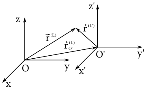
Figure 1: Laboratory coordinate systems $L$ and $L^{\prime}$.

Let us introduce the following notation: $m_{1}=m_{n}$ is the neutron mass; $m_{2}=m_{N}$ is the nucleus mass; $\vec{r}_{1}^{(L)}$ is the neutron radius vector in the $L$-system; $\vec{r}_{2}^{(L)}$ is the nucleus radius vector in the $L$-system; $\vec{r}_{c}^{(L)}$ is the radius vector of the center of mass in the $L$-system; $\vec{r}_{1}^{(L^{\prime})}$ is the neutron radius vector in the $L^{\prime}$-system; $\vec{r}_{2}^{(L^{\prime})}$ is the nucleus radius vector in the $L^{\prime}$-system; $\vec{V}_{10}^{(L)}$ is the neutron speed in the $L$-system before the collision with the nucleus; $\vec{V}_{1}^{(L)}$ is the neutron speed in the $L$-system after the collision with a nucleus; $\vec{V}_{20}^{(L)}$ is the nucleus speed in the $L$-system before the collision with a neutron; $\vec{V}_{2}^{(L)}$ is the nucleus speed in the $L$-system after the collision with a neutron; $\vec{V}_{10}^{(L^{\prime})}$ is the neutron speed in the $L^{\prime}$-system before the collision with the nucleus; $\vec{V}_{1}^{(L^{\prime})}$ is the neutron speed in the $L^{\prime}$-system after the collision with a nucleus; $\vec{V}_{20}^{(L^{\prime})}$ is the nucleus speed in the $L^{\prime}$-system before the collision with a neutron; $\vec{V}_{2}^{(L^{\prime})}$ is the nucleus speed in the $L^{\prime}$-system after the collision with a neutron; $\vec{V}_{c}^{(L^{\prime})}$ is the speed of the center of mass in the $L^{\prime}$-system.

The radius vectors of a point in the laboratory coordinate systems $L$ and $L^{\prime}$ are connected by the following equation:

$$\vec{r}^{(L)}=\vec{r}_{O^{\prime}}^{(L)}+\vec{r}^{(L^{\prime})}$$ (1)

Thus, in accordance with our aim, we can write that

$$\vec{V}_{10}^{(L)}=\frac{d\vec{r}_{1}^{(L)}}{dt}\neq 0~{}\text{and}~{}\vec{V}_{20}^{(L)}=\frac{d\vec{r}_{2}^{(L)}}{dt}\neq 0$$ (2)

and choose the $L^{\prime}$-system so that the nucleus rest in it before the collision:

$$\vec{V}_{20}^{(L^{\prime})}=0$$ (3)

The relationship between the coordinates of $m_{1}$ and $m_{2}$ in the $L$-system and the $L^{\prime}$-system is given by (1), and between the speeds – by the following expressions (the Galilean law):

$$\vec{V}_{1}^{(L^{\prime})}=\vec{V}_{1}^{(L)}-\vec{V}_{20}^{(L)}~{}\text{and}~{}\vec{V}_{2}^{(L^{\prime})}=\vec{V}_{2}^{(L)}-\vec{V}_{20}^{(L)}$$ (4)

It is convenient to solve the problem of the two particles collision in the coordinate system associated with the mass center – the $C$-system.

On the basis of the momentum conservation law, for the two colliding particles in the $C$-system we obtain:

$$\vec{P}_{10}^{(C)}+\vec{P}_{20}^{(C)}=\vec{P}_{1}^{(C)}+\vec{P}_{2}^{(C)}=0$$ (5)

From the relations (5) follows:

$$m_{1}\cdot\vec{V}_{10}^{(C)}=-m_{2}\cdot\vec{V}_{20}^{(C)}~{}\text{and}~{}m_{1}\cdot\vec{V}_{1}^{(C)}=-m_{2}\cdot\vec{V}_{2}^{(C)}$$ (6)

From (6) we obtain the speed moduli:

$$\left|\vec{V}_{10}^{(C)}\right|=V_{10}^{(C)}=\frac{m_{2}}{m_{1}}\left|\vec{V}_{20}^{(C)}\right|=\frac{m_{2}}{m_{1}}V_{20}^{(C)}~{}\text{and}~{}V_{1}^{(C)}=\frac{m_{2}}{m_{1}}V_{2}^{(C)}$$ (7)

Introducing the mass number for the neutron and the nucleus $A_{n}=1$ and $A_{N}=A$, respectively, and assuming that $m_{1}=m_{n}\approx A_{n}=1$ and $m_{2}=m_{N}\approx A_{N}=A$, for the Eqs. (6) and (7) we obtain the following expressions:

$$\vec{V}_{10}^{(C)}=-A\cdot\vec{V}_{20}^{(C)}~{}\text{and}~{}\vec{V}_{1}^{(C)}=-A\cdot\vec{V}_{2}^{(C)}$$ (8)

and

$$V_{10}^{(C)}=+A\cdot V_{20}^{(C)}~{}\text{and}~{}V_{1}^{(C)}=+A\cdot V_{2}^{(C)}$$ (9)

From the kinetic energy conservation law in the C-system we obtain:

$$\frac{\left(V_{10}^{(C)}\right)^{2}}{2}+\frac{A\cdot\left(V_{20}^{(C)}\right)^{2}}{2}=\frac{\left(V_{1}^{(C)}\right)^{2}}{2}+\frac{A\cdot\left(V_{2}^{(C)}\right)^{2}}{2}.$$ (10)

Hence, in view of (9) and (10) we obtain the following relation:

$$\left(V_{10}^{(C)}\right)^{2}\cdot\left(1+\frac{1}{A}\right)=\left(V_{1}^{(C)}\right)^{2}\cdot\left(1+\frac{1}{A}\right).$$ (11)

From (11) it follows that:

$$V_{10}^{(C)}=V_{1}^{(C)}.$$ (12)

Also, from the kinetic energy conservation law (10), taking into account the relation (12) it follows:

$$V_{20}^{(C)}=V_{2}^{(C)}.$$ (13)

Thus we can see that in the $C$-system of the closed mechanical system consisting of the neutron and the nucleus, the neutron and the nucleus move along a straight line connecting their centers (towards each other before the collision and in the opposite directions after collision) (see (6)). They also decline at certain angle $\theta$ while maintaining the absolute values of their velocities (see (12) and (13), Fig. 2).

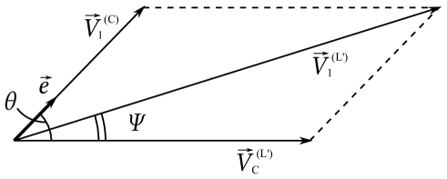
Figure 2: Fig.2. Parallelogram of velocities after the collision in the $L^{\prime}$ coordinate system.

The center of mass coordinate of the neutron and the moderating medium nucleus ($\vec{r}_{c}^{(L^{\prime})}$ is the radius vector of the center of mass in the $L^{\prime}$ laboratory coordinate system) may be given as:

$$\vec{r}_{c}^{(L^{\prime})}=\left(1\cdot\vec{r}_{1}^{(L^{\prime})}+A\cdot\vec{r}_{2}^{(L^{\prime})}\right)\cdot\frac{1}{A+1}$$ (14)

where $\vec{r}_{1}^{(L^{\prime})}$ is the radius vector of the neutron in the $L^{\prime}$-system; $\vec{r}_{2}^{(L^{\prime})}$ is the radius vector of the nucleus; $A$ is the mass number of the nucleus; $1$ is the mass number of a neutron.

Given the fact that in the $L^{\prime}$-system the nucleus velocity before the collision $\vec{V}_{20}^{(L^{\prime})}=0$, the velocity of the mass center of a closed system of two particles (the neutron and the nucleus) in the $L^{\prime}$ coordinate system is:

$$\vec{V}_{C}^{(L^{\prime})}=\frac{1}{A+1}\cdot\vec{V}_{10}^{(L^{\prime})}.$$ (15)

By virtue of the law of the total momentum conservation, the velocity of the inertia center in the $L^{\prime}$-system will not change after the collision. Therefore the indices corresponding to the velocity values of the inertia center before the interaction and after the interaction may be omitted.

Since the mass center system ($C$-system) moves relative to the laboratory system with the speed of the center of mass in the $L^{\prime}$-system, for the velocity of the neutron in the $C$-system before the interaction we have:

$$\vec{V}_{10}^{(C)}=\vec{V}_{10}^{(L^{\prime})}-\vec{V}_{C}^{(L^{\prime})},$$ (16)

then we substitute the expression (15) into this expression and obtain:

$$\vec{V}_{10}^{(C)}=\vec{V}_{10}^{(L^{\prime})}-\frac{1}{A+1}\cdot\vec{V}_{10}^{(L^{\prime})}=\frac{A}{A+1}\cdot\vec{V}_{10}^{(L^{\prime})}.$$ (17)

Using the Eq. (5) with regard for the expression (17), we find the speed of the nucleus in the $C$-system before the collision:

$$\vec{V}_{10}^{(C)}=-\frac{1}{A+1}\cdot\vec{V}_{10}^{(L^{\prime})}.$$ (18)

According to (12), (13) and using the expressions (17) and (18) we obtain:

$$V_{1}^{(C)}=V_{10}^{(C)}=\frac{A}{A+1}\cdot V_{10}^{(L^{\prime})}~{}\text{and}~{}V_{2}^{(C)}=V_{20}^{(C)}=\frac{1}{A+1}\cdot V_{10}^{(L^{\prime})}.$$ (19)

These results should be adapted to the $L^{\prime}$ coordinate system. The neutron velocity in the $L^{\prime}$ laboratory coordinate system after the collision is:

$$\vec{V}_{1}^{(L^{\prime})}=\vec{V}_{1}^{(C)}+\vec{V}_{C}^{(L^{\prime})},$$ (20)

Taking into account (15), for (20) we obtain:

$$\vec{V}_{1}^{(L^{\prime})}=\vec{V}_{1}^{(C)}+\frac{1}{A+1}\cdot\vec{V}_{10}^{(L^{\prime})}.$$ (21)

The neutron velocity in the $L^{\prime}$-system after the collision is directed at an angle $\Psi$ to the original direction (Fig. 2).

From the parallelogram of velocities shown in Fig. 2 we find the squared modulus of the neutron velocity in the $L^{\prime}$-system after the collision:

$$\left(\vec{V}_{1}^{(L^{\prime})}\right)^{2} =\left(V_{10}^{(L^{\prime})}\cdot\frac{A}{A+1}\right)^{2}+\left(V_{10}^{(L^{\prime})}\cdot\frac{1}{A+1}\right)^{2}+\frac{2\cdot A\cdot\left(V_{10}^{(L^{\prime})}\right)^{2}}{(A+1)^{2}}\cdot\cos{\theta}=$$

$$=\frac{\left(V_{10}^{(L^{\prime})}\right)^{2}\cdot(A^{2}+2A\cos{\theta}+1)}{(A+1)^{2}},$$ (22)

where $\theta$ is the angle of the neutron escape in the $C$-system (Fig. 2).

From (22) it is possible to find the ratio of the squares of the velocities before and after neutron interaction with the nucleus in the $L^{\prime}$ laboratory coordinate system, which is also equal to the ratio of the kinetic energies of the neutron before and after the interaction:

$$\frac{\left(\vec{V}_{1}^{(L^{\prime})}\right)^{2}}{\left(\vec{V}_{10}^{(L^{\prime})}\right)^{2}}=\frac{E_{2}^{(L^{\prime})}}{E_{1}^{(L^{\prime})}}=\frac{A^{2}+2A\cos{\theta}+1}{(A+1)^{2}},$$ (23)

where $E_{1}$ and $E_{2}$ are the kinetic energies of the neutron before and after the collision in the $L^{\prime}$-system respectively.

Let us introduce the parameter

$$\alpha=\left(\frac{A-1}{A+1}\right)^{2},$$ (24)

then (1) may be given in the following widely-known form [5, 6]:

$$\frac{E_{2}^{(L^{\prime})}}{E_{1}^{(L^{\prime})}}=\frac{1}{2}\left[(1+\alpha)+(1-\alpha)\cos{\theta}\right].$$ (25)

The maximum value of $E_{2}^{(L^{\prime})}/E_{1}^{(L^{\prime})}$ corresponds to the value $\theta=0$. This the minimum loss of energy, i.e. the neutron does not lose its energy in a collision. When $\theta=\pi$ (central collision) $E_{2}^{(L^{\prime})}/E_{1}^{(L^{\prime})}=\alpha$. The minimum value to which the neutron energy may reduce as a result of a single elastic scattering is $\alpha E_{1}^{(L^{\prime})}$.

The maximum relative energy loss in a single scattering is

$$\frac{E_{1}^{(L^{\prime})}-E_{2}^{(L^{\prime})}}{E_{1}^{(L^{\prime})}}=1-\alpha,$$ (26)

and the maximum possible absolute energy loss is

$$E_{1}^{(L^{\prime})}(1-\alpha).$$ (27)

$\alpha=0$ for hydrogen, i.e. the neutron can lose all its kinetic energy in a single collision event with a hydrogen nucleus. If we expand $\alpha$ in powers of $\frac{1}{A}$, we obtain:

$$\alpha=1-\frac{4}{A}+\frac{8}{A^{2}}-\frac{12}{A^{3}}+\ldots$$ (28)

At $A>50$

$$\alpha\approx 1-\frac{4}{A},~{}~{}~{}\text{a}~{}~{}~{}1-\alpha\approx\frac{4}{A}.$$ (29)

It is evident that the smaller is $A$, the greater is the relative energy loss. Thus the moderation is more effective for the nuclei with small $A$. When $A>200$, $(1-\alpha)<2\%$. It means that uranium may not be considered a moderator in nuclear reactors.

Next we use the Eq. (4) connecting the neutron velocities in the $L^{\prime}$ and $L$ coordinate systems, and the ratio (25), to give the relation (23) in the following form:

$$\frac{\left(\vec{V}_{1}^{(L)}-\vec{V}_{20}^{(L)}\right)^{2}}{\left(\vec{V}_{10}^{(L)}-\vec{V}_{20}^{(L)}\right)^{2}}=\frac{A^{2}+2A\cos{\theta}+1}{(A+1)^{2}}=\frac{1}{2}\left[(1+\alpha)+(1-\alpha)\cos{\theta}\right].$$ (30)

From (30) after some algebraic manipulations it is possible to find the ratio of the squares of the neutron velocity before and after the interaction with the nucleus in the $L$-system. It is also equal to the ratio of the kinetic energy of the neutron before and after the interaction.

$$\frac{\left(\vec{V}_{1}^{(L)}\right)^{2}}{\left(\vec{V}_{10}^{(L)}\right)^{2}} =\frac{E_{1}^{(L)}}{E_{10}^{(L)}}=\frac{1}{2}\left[(1+\alpha)+(1-\alpha)\cos{\theta}\right]\left[1-2\frac{V_{10}^{(L)}V_{20}^{(L)}\cos{\beta}}{\left(V_{10}^{(L)}\right)^{2}}+\frac{\left(V_{20}^{(L)}\right)^{2}}{\left(V_{10}^{(L)}\right)^{2}}\right]+$$

$$+2\frac{\left(\vec{V}_{1}^{(L)},\vec{V}_{20}^{(L)}\right)}{\left(V_{10}^{(L)}\right)^{2}}-\frac{\left(V_{20}^{(L)}\right)^{2}}{\left(V_{10}^{(L)}\right)^{2}}=\frac{1}{2}\left[(1+\alpha)+(1-\alpha)\cos{\theta}\right]-$$

$$-\left[(1+\alpha)+(1-\alpha)\cos{\theta}\right]\frac{V_{10}^{(L)}V_{20}^{(L)}\cos{\beta}}{\left(V_{10}^{(L)}\right)^{2}}+2\frac{V_{1}^{(L)}V_{20}^{(L)}\cos{\gamma}}{\left(V_{10}^{(L)}\right)^{2}}-$$

$$-\left\{1-\frac{1}{2}\left[(1+\alpha)+(1-\alpha)\cos{\theta}\right]\right\}\frac{1\cdot E_{20}^{(L)}}{A\cdot E_{10}^{(L)}},$$ (31)

where $\cos{\beta}$ is the cosine of the angle between the vectors $\vec{V}_{10}^{(L)}$ and $\vec{V}_{20}^{(L)}$ which is given by the scalar product of these vectors $\left(\vec{V}_{10}^{(L)},\vec{V}_{20}^{(L)}\right)$ as follows:

$$\cos{\beta}=\frac{\left(\vec{V}_{10}^{(L)},\vec{V}_{20}^{(L)}\right)}{\left|\vec{V}_{10}^{(L)}\right|\left|\vec{V}_{20}^{(L)}\right|}=\frac{\left(\vec{V}_{10}^{(L)},\vec{V}_{20}^{(L)}\right)}{V_{10}^{(L)}V_{20}^{(L)}},$$ (32)

$\cos{\gamma}$ is the cosine of the angle between the vectors $\vec{V}_{1}^{(L)}$ and $\vec{V}_{20}^{(L)}$ which is given by the scalar product of these vectors $\left(\vec{V}_{1}^{(L)},\vec{V}_{20}^{(L)}\right)$ as follows:

$$\cos{\gamma}=\frac{\left(\vec{V}_{1}^{(L)},\vec{V}_{20}^{(L)}\right)}{\left|\vec{V}_{1}^{(L)}\right|\left|\vec{V}_{20}^{(L)}\right|}=\frac{\left(\vec{V}_{1}^{(L)},\vec{V}_{20}^{(L)}\right)}{V_{1}^{(L)}V_{20}^{(L)}},$$ (33)

Let us note that from (31) it follows that, since the $\cos{\beta}$ and $\cos{\gamma}$ may take both the positive and negative values, the energy of a scattered neutron may be both smaller and greater than its initial energy. This is because some part of the kinetic energy of the nucleus may be transferred to neutron during the scattering.

As will be shown below, for our purposes it is sufficient to limit oneself to Eq. (39) and not perform the rest of the transformations of the Eq. (31) and related Eqs. (32) and (33), since they contain the cosines of the angles between the neutron and nucleus velocity vectors, which also require the adaptation to the $L$-system.

3 The neutron scattering law taking into account the thermal motion of the moderating medium nuclei

According to the kinematics of the neutron scattering by a nucleus, shown in section 2, the probability for a neutron with kinetic energy $E_{10}^{(L)}$ before scattering in the $L$-system to possess the kinetic energy in the range from $E_{1}^{(L)}$ to $E_{1}^{(L)}+dE_{1}^{(L)}$ after the scattering may be written as follows:

$$P\left(E_{1}^{(L)}\right)dE_{1}^{(L)} =P\left(\theta,\beta,\gamma,E_{N}^{(L)}\right)d\theta d\beta d\gamma dE_{N}^{(L)}=$$

$$=P(\theta)d\theta\cdot P(\beta)d\beta\cdot P(\gamma)d\gamma\cdot P\left(E_{N}^{(L)}\right)dE_{N}^{(L)}.$$ (34)

From the quantum mechanical scattering theory it is known (e.g. [4, 24]) that if the de Broglie wavelength is much larger than the size of the nucleus, the neutron scattering by a potential well of the nucleus must be spherically symmetric in the center of inertia coordinate system ($C$-system), i.e. isotropic. It is useful to estimate the threshold neutron energy $E_{B}$ above which the neutron scattering is not spherically symmetric. According to [4], this can be done using the quasiclassical approximation in the quantum-mechanical problem of the neutron scattering by a potential well of the nucleus. Let $R$ be the effective radius of the nucleus, $\rho$ – the impact parameter of the incident neutron, $v$ – its speed. As in the classical representation of the orbital angular momentum of the neutron $\rho v=l\hbar(l=0,1,2,\ldots)$, the scattering should take place at $Rv\geqslant\rho v=l\hbar$. The scattering is spherically symmetric if $l=0$, and only if $l\geqslant 1$, the scattering is the anisotropic. Therefore, for the anisotropic scattering the condition $Rv\geqslant\hbar$ must be satisfied, which implies that $v_{B}\geqslant\hbar/R$. Since $E_{B}=mv^{2}/2$, where $m$ is the neutron mass, and the nucleus radius may be expressed as a well known expression $R\approx r_{0}A^{1/3}$, where $r_{0}=1.2\cdot 10^{-13}$cm, $A$ is the mass number of the scattering nucleus, the neutron energy threshold is

$$E_{B}=\frac{\hbar^{2}}{2mr_{0}^{2}}\frac{1}{A^{2/3}}\sim\frac{10~{}MeV}{A^{2/3}}.$$ (35)

Thus, according to (35) for hydrogen as moderator, almost the entire range of fission spectrum (0 - 10 MeV) is the range of the spherically symmetric scattering of neutrons in the $C$-system. For carbon ($A$ = 12) we obtain that $E_{B}\sim 2~{}MeV$. Because the average energy of the fission neutron spectrum is $\sim 2~{}MeV$, it gives a reason to believe that the neutron moderation by the light nuclei, the scattering is spherically symmetric in the $C$-system.

These estimates are confirmed by the experimental data, e.g. [5], the neutron scattering is spherically symmetric in the center of mass coordinate system (isotropic) up to the neutron energy $\sim 10^{5}~{}eV$.

Thus, since the scattering of neutrons in the center of mass coordinate system is spherically symmetric (isotropic), then for $P(\theta)d\theta$ we obtain:

$$P(\theta)d\theta=\int\limits_{0}^{2\pi}\left[P(\theta,\varphi)d\theta\right]d\varphi=\int\limits_{0}^{2\pi}\frac{r\sin{\theta}d\varphi\cdot rd\theta}{4\pi r^{2}}=\frac{\sin{\theta}d\theta}{4\pi}\int\limits_{0}^{2\pi}d\varphi=\frac{1}{2}\sin{\theta}d\theta,$$ (36)

where $\varphi$ is the azimuth angle of the usual spherical coordinates $r,\theta,\varphi$ introduced in the center of mass coordinate system.

Since the thermal motion of the moderating medium nuclei is chaotic, and the neutron source is isotropic, the distribution of the velocity vector directions in the space for the neutrons after the collision is equiprobable over the $\beta$ and $\gamma$ angles, i.e. also spherically symmetric (isotropic). So by analogy we obtain:

$$P(\beta)d\beta=\frac{1}{2}\sin{\beta}d\beta,$$ (37)

$$P(\gamma)d\gamma=\frac{1}{2}\sin{\gamma}d\gamma,$$ (38)

By averaging the neutron kinetic energy after scattering given by the expression (31) over the spherically symmetric distribution of the moderator nuclei thermal motion and isotropic neutron source, we obtain the following expression:

$$\bar{E}_{1}^{(L)} =\int\limits_{0}^{\pi}\int\limits_{0}^{\pi}E_{1}^{(L)}\cdot P(\beta)d\beta\cdot P(\gamma)d\gamma=$$

$$=\bar{E}_{10}^{(L)}\left\{\frac{1}{2}\left[(1+\alpha)+(1-\alpha)\cos{\theta}\right]-\left[1-\frac{1}{2}\left[(1+\alpha)+(1-\alpha)\cos{\theta}\right]\frac{E_{N}^{(L)}}{A\cdot\bar{E}_{10}^{(L)}}\right]\right\}.$$ (39)

Here $\bar{E}_{10}^{(L)}$ is the neutron energy averaged over the neutron momenta directions for the isotropic neutron source (coincides with the neutron energy $\bar{E}_{10}^{(L)}=E_{10}^{(L)}$), $E_{N}^{(L)}$ is defined by the Maxwell distribution [25] for the moderator nuclei, which depends on the moderating medium temperature:

$$P\left(E_{N}^{(L)}\right)dE_{N}^{(L)}=\frac{2}{\sqrt{\pi(kT)^{3}}}e^{-\frac{E_{N}^{(L)}}{kT}}\sqrt{E_{N}^{(L)}}dE_{N}^{(L)}.$$ (40)

Let us average the expression (39) over the Maxwellian distribution of the thermal motion of the moderating medium nuclei (40), considering that $\bar{E}_{10}^{(L)}=E_{10}^{(L)}$. If we use a well-known result $\bar{E}_{N}^{(L)}=\int\limits_{0}^{\infty}E_{N}^{(L)}P_{M}\left(E_{N}^{(L)}\right)dE_{N}^{(L)}=\frac{3}{2}kT$ [25], we obtain the following expression:

$$\bar{\bar{E}}_{1}^{(L)} =\int\limits_{0}^{\infty}\bar{E}_{1}^{(L)}P_{M}\left(E_{N}^{(L)}\right)dE_{N}^{(L)}=$$

$$=E_{10}^{(L)}\left\{\frac{1}{2}\left[(1+\alpha)+(1-\alpha)\cos{\theta}\right]-\left[1-\frac{1}{2}\left[(1+\alpha)+(1-\alpha)\cos{\theta}\right]\frac{\frac{3}{2}kT}{A\cdot E_{10}^{(L)}}\right]\right\}$$ (41)

Since the functional relationship between $\bar{\bar{E}}_{1}^{(L)}$ and $\theta$ unique, as follows from (41), the probability $P\left(\bar{\bar{E}}_{1}^{(L)}\right)dE_{1}^{(L)}$ for the neutron with a kinetic energy $E_{10}^{(L)}$ in the $L$-system before scattering to possess the kinetic energy in the range from $\bar{\bar{E}}_{1}^{(L)}$ to $\bar{\bar{E}}_{1}^{(L)}+dE_{1}^{(L)}$ after the scattering on the chaotically moving moderator nuclei is determined by the $P(\theta)d\theta$ distribution (36). Therefore we obtain the following relation (here we omit the symbols of averaging and the laboratory coordinate system $L$ for simplicity, i.e. $P\left(\bar{\bar{E}}_{1}^{(L)}\right)dE_{1}^{(L)}=P(E_{1})dE_{1}$):

$$P(E_{1})dE_{1} =P(\theta)d\theta=P(\theta)\left|\frac{d\theta}{dE_{1}}\right|dE_{1}=$$

$$=\frac{1}{2}\sin{\theta}\left|\frac{1}{E_{10}^{(L)}\left[\frac{1}{2}(1-\alpha)\sin{\theta}+\frac{1}{2}(1-\alpha)\sin{\theta}\frac{\frac{3}{2}kT}{A\cdot E_{10}^{(L)}}\right]}\right|dE_{1}=$$

$$=\frac{dE_{1}}{\left[E_{10}^{(L)}+\frac{1}{A}\cdot\frac{3}{2}kT\right](1-\alpha)}$$ (42)

Thus, we obtained the neutron scattering law, which takes into account the thermal motion of the moderating medium nuclei:

$$\begin{cases}P(E_{1})dE_{1}=\frac{dE_{1}}{\left[E_{10}^{(L)}+\frac{1}{A}\frac{3}{2}kT\right](1-\alpha)}&\text{when}~{}~{}\alpha\left(E_{10}^{(L)}+\frac{1}{A}\frac{3}{2}kT\right)\leqslant E_{1}\leqslant\left(E_{10}^{(L)}+\frac{1}{A}\frac{3}{2}kT\right)\\ P(E_{1})=0&\text{when}~{}~{}E_{1}\leqslant\alpha\left(E_{10}^{(L)}+\frac{1}{A}\frac{3}{2}kT\right)~{}\text{,}~{}E_{1}\geqslant\left(E_{10}^{(L)}+\frac{1}{A}\frac{3}{2}kT\right)\end{cases}$$ (43)

In conclusion of the section, let us emphasize that the new scattering law (43) is written for the averaged neutron energy after scattering $E_{1}$. The averaging of the neutron energy is performed over the thermal (chaotic) motion of the moderating medium nuclei and the neutron source isotropy.

It should also be noted that although (as mentioned in section 2 above) the relation (31) implies that the individual neutrons may receive an additional energy as a result of scattering, the scattering law for an isotropic neutron source (43), averaged over the thermal motion of the moderating medium nuclei and neutron source isotropy yields the energy of a group of neutrons after scattering almost always smaller than the averaged energy of a group of neutrons before scattering. It means that this is actually the neutron moderation law, but now taking into account the thermal motion of the moderating medium nuclei and the isotropy of the neutron source.

Let us also mention some ”tricks” or ”moves” it was necessary to take in order to obtain the neutron moderation law in the form of (43), since the previous attempts failed without them (e.g. an attempt by Galanin [3]):

• the first move is the transition from the $L$ laboratory coordinate system to the $L^{\prime}$ laboratory coordinate system, in which the moderator nucleus rests (section 2). Thus the kinematics of the standard moderation theory leading to the expression (30) may be applied;

• the second move is the inverse transition from the $L^{\prime}$ coordinate system to the $L$-system transforming (30) into (31);

• the third move is the averaging of the expression (31) over the thermal motion of the nuclei, which gives (41);

• the fourth move is the derivation of the scattering law (43).

As we shall see below, the scattering law (43) lets one derive the expressions for the flux and energy spectra of the moderating neutrons in a variety of media, taking into account the temperature of the medium.

In order to take the neutron scattering anisotropy into account, a transport macroscopic cross-section is introduced in the nuclear reactor physics [4, 5, 6]:

$$\Sigma_{tr}=\Sigma_{a}+\Sigma_{s}(1-\bar{\mu}),$$ (44)

where $\Sigma_{a}$ and $\Sigma_{s}$ are the macroscopic absorption cross-section and the macroscopic scattering cross-section of neutrons respectively, $\bar{\mu}$ is the average cosine of the scattering angle. If $\Sigma_{a}\ll\Sigma_{s}$, then

$$\Sigma_{tr}\approx\Sigma_{s}(1-\bar{\mu}).$$ (45)

For small deviations from spherical symmetry typical for the reactor neutrons, i.e. for the scattering anisotropy, which may be observed during the scattering of the high-energy neutrons by the moderators with heavy nuclei, the scattering law, according to [5], may be given as follows:

$$\begin{cases}P(E_{1})dE_{1}=\frac{dE_{1}}{\left[E_{10}^{(L)}+\frac{1}{A}\cdot\frac{3}{2}kT\right](1-\alpha)}\left[1+3\bar{\mu}-\frac{6}{(1-\alpha)}\bar{\mu}\frac{E_{1}-E_{10}^{(L)}}{E_{1}}\right]&\text{when}~{}~{}\alpha E_{10}^{(L)}\leqslant E_{1}\leqslant E_{10}^{(L)}\\ P(E_{1})=0&\text{when}~{}~{}E_{1}\leqslant\alpha E_{10}^{(L)}~{}~{}\text{and}~{}~{}E_{1}\geqslant E_{10}^{(L)}\end{cases}$$ (46)

where

$$\bar{\mu}=0.07\cdot A^{2/3}E~{}~{}~{}\text{when}~{}~{}l=1~{}~{}~{}\text{(see the beginning of this section)}.$$ (47)

In contrast to the scattering law for isotropic scattering (43), the probability $P(E_{1})$ depends on the final neutron energy $E_{1}$ in the scattering law (46).

It is also obvious that at neutron energies tending to zero, the gas model considered here stops working, and it is necessary to develop a moderation theory taking into account the interaction between the nuclei (ions or molecules) of a moderator.

4 Neutron moderation in hydrogen media without absorption

According to the scattering law (43), the neutron moderation law in the non-absorbing hydrogen media ($\alpha=0$ and $A=1$) has the following form:

$$P(E_{1})dE_{1}=\frac{dE_{1}}{\left[E_{10}^{(L)}+\frac{3}{2}kT\right]}$$ (48)

Performing the calculations similar to those in [4, 5, 6], using the moderation law (48) we find the following expression for the moderating neutrons flux density (here the new notation is introduced $E=E_{10}^{(L)}$ and $dE=dE_{1}$ for the sake of simplification):

$$\Phi(E)=\frac{\int\limits_{E}^{\infty}Q(E^{\prime})dE^{\prime}}{\left[E+\frac{3}{2}kT\right]\Sigma_{s}(E)}+\frac{Q(E)}{\Sigma_{s}(E)},$$ (49)

where $Q(E^{\prime})$ is the number of neutrons generated per unit volume per unit time with the energy $E^{\prime}$.

Indeed, according to the neutron scattering law (43), the energy of neutrons having an initial energy $E$ will be distributed equiprobably in the range from $E$ to $0$ after a collision with hydrogen nuclei.

If we divide this energy range from $E$ to $0$ into intervals of size $dE$, the number of neutrons scattered in the interval $dE$ as a result of scattering collisions in the range $dE$ in the vicinity of the energy $E$ will be:

$$\Phi(E)\Sigma_{s}(E)dE=\frac{dE}{E+\frac{3}{2}kT}=F(E)dE\frac{dE}{E+\frac{3}{2}kT},$$ (50)

where $F(E)$ denotes the number of the acts of neutron scattering with energy $E$ per unit volume per unit time.

The total number of neutrons scattered into the energy range $dE$ as a result of all collisions of this type in the energy range from the initial neutron energy $E_{10}$ to $E$ is

$$dE\int\limits_{E}^{E_{10}}\frac{F(E^{\prime})dE^{\prime}}{E^{\prime}+\frac{3}{2}kT}.$$ (51)

It is assumed here that the neutrons had been scattered into the interval $dE$ in the vicinity of the energy $E$, and only after that they were scattered into the interval $dE$. However, since a single collision with a hydrogen nucleus can reduce the neutron energy from its initial value $E_{10}$ to $0$, some neutrons are apparently scattered into the interval $dE$ as a result of their first collision.

A monoenergetic (discrete energy) neutron source can be written mathematically as

$$Q(E)=Q_{0}\delta(E-E_{10})$$ (52)

where $Q_{0}=Q(E_{10})$ is the number of generated neutrons with the energy $E_{10}$ per unit volume per unit time, $\delta(E-E_{10})$ is the generalized Dirac function.

As for the case of non-monoenergetic neutron source (continuous spectrum with a maximum of neutron energy of $E_{max}$), the total number of neutrons scattered into an interval of energy $dE$ near the energy $E$ is

$$dE\left[\int\limits_{E}^{E_{max}}\left(\int\limits_{E}^{E_{10}}\frac{F(E^{\prime})dE^{\prime}}{E^{\prime}+\frac{3}{2}kT}+Q(E_{10})\delta(E-E_{10})\right)dE_{10}\right]=$$

$$=dE\left[\int\limits_{E}^{E_{max}}\left(\int\limits_{E}^{E_{10}}\frac{F(E^{\prime})dE^{\prime}}{E^{\prime}+\frac{3}{2}kT}\right)dE_{10}+Q(E)\right].$$ (53)

The number of the neutrons leaving interval of energies $dE$ near $E$ due to scattering is equal to $F(E)dE$, so the non-stationary neutron balance equation for the interval of energies $dE$ near $E$ is

$$\frac{\partial n(E,t)}{\partial t}dE=dE\left[\int\limits_{E}^{E_{max}}\left(\int\limits_{E}^{E_{10}}\frac{F(E^{\prime})dE^{\prime}}{E^{\prime}+\frac{3}{2}kT}\right)dE_{10}+Q(E)\right]-F(E)dE.$$ (54)

The non-stationary integro-differential equation (54) cannot be solved analytically, and its solutions may only be found numerically. Of course, in the future we will work on the development of the theory of non-stationary moderation process, but in this paper we will focus on a more simple stationary case.

The condition of the stationarity of the neutron energy distribution means that the number of neutrons leaving each elementary energy interval as a result of the scattering should be equal to the total number of neutrons entering the same interval. The number of neutrons leaving the interval $dE$ due to scattering is $F(E)dE$, so the condition of stationarity for interval $dE$ may be written as

$$F(E)dE=dE\left[\int\limits_{E}^{E_{max}}\left(\int\limits_{E}^{E_{10}}\frac{F(E^{\prime})dE^{\prime}}{E^{\prime}+\frac{3}{2}kT}\right)dE_{10}+Q(E)\right].$$ (55)

Equation (55) in the case of a stationary moderation spectrum is equivalent to the following equation:

$$F(E)dE=\left[\int\limits_{E}^{E_{10}}\frac{F(E^{\prime})dE^{\prime}}{E^{\prime}+\frac{3}{2}kT}+Q(E)\right]dE.$$ (56)

According to [4, 5, 6], the integral equation (56) may be reduced to a differential equation with the following solution:

$$F(E)=\frac{\int\limits_{E}^{E_{max}}Q(E^{\prime})dE^{\prime}}{\left[E+\frac{3}{2}kT\right]}+Q(E).$$ (57)

Indeed, if we differentiate (56) with respect to energy $E$, we obtain

$$\frac{dF(E)}{dE}=-\frac{F(E)}{\left[E+\frac{3}{2}kT\right]}+\frac{dQ(E)}{dE}.$$ (58)

By putting the derivatives into left hand side, we obtain a non-homogeneous differential equation

$$\frac{d\left[F(E)-Q(E)\right]}{dE}=-\frac{F(E)}{\left[E+\frac{3}{2}kT\right]}.$$ (59)

According to the differential equation theory, the general solution of a non-homogeneous differential equation (59) is a sum of the solution of the corresponding homogeneous differential equation, which may be obtained from (59) by zeroing out its right-hand side, and some particular solution of the non-homogeneous equation (59).

Let us first find a solution of the homogeneous equation of the form

$$\frac{d\left[F(E)-Q(E)\right]}{dE}=0.$$ (60)

The solution of the Eq. (60) may be easily found, and has the following form:

$$F(E)=Q(E)+const.$$ (61)

Now let us find a particular solution of the non-homogeneous equation (59). For this purpose let us perform the gradient calibration, i.e. switch from the function $F(E)$ to the function $F^{\prime}(E)$ related to $F(E)$ in the following way:

$$F(E)=F^{\prime}(E)+f(E),$$ (62)

where $f(E)$ is the calibration function which must fullfill the calibration equation we shall derive below.

Let us substitute the expression (62) into non-homogeneous equation (59) end obtain the following:

$$\frac{dF^{\prime}(E)}{dE}+\frac{df(E)}{dE}-\frac{dQ(E)}{dE}=-\frac{F^{\prime}(E)}{\left[E+\frac{3}{2}kT\right]}-\frac{f(E)}{\left[E+\frac{3}{2}kT\right]}.$$ (63)

We impose the following condition for the calibration function $f(E)$:

$$\frac{df(E)}{dE}-\frac{dQ(E)}{dE}+\frac{f(E)}{\left[E+\frac{3}{2}kT\right]}=0.$$ (64)

Then from (63) we obtain a system of two equations

$$\frac{dF^{\prime}(E)}{dE}=-\frac{F^{\prime}(E)}{\left[E+\frac{3}{2}kT\right]},$$ (65)

$$\frac{d\left[f(E)-Q(E)\right]}{dE}=-\frac{f(E)}{\left[E+\frac{3}{2}kT\right]}.$$ (66)

Let us find the solution to the equation (65). Its solution has the form

$$F^{\prime}(E)=\frac{C_{1}}{\left[E+\frac{3}{2}kT\right]},$$ (67)

where $C_{1}$ is an arbitrary constant.

Now let us consider Eq. (66) for $f(E)$. Its form coincides with that of the non-homogeneous differential equation (59) for $F(E)$. Thus the particular solution for the Eq. (66) may be given as follows:

$$f(E)=C_{2}\cdot F(E),$$ (68)

where $C_{2}$ is an arbitrary constant.

Substituting the solution (68) into (62), we obtain the following expression for $F(E)$:

$$F(E)=F^{\prime}(E)+C_{2}\cdot F(E),$$ (69)

From (69) for $F(E)$ we obtain:

$$F(E)=F^{\prime}(E)/C_{3},$$ (70)

where $C_{3}=(1-C_{2})$ is a non-zero constant.

Further substituting the solution (67) into (70), for the particular solution of the non-homogeneous differential equation (59) $F(E)$ we have:

$$F(E)=\frac{C_{4}}{\left[E+\frac{3}{2}kT\right]},$$ (71)

where $C_{4}=C_{1}/C_{3}$ is a constant.

Thus, having the solution (61) of the homogeneous differential equation and the particular solution of the non-homogeneous equation (71), we can write down the general solution of the equation (59):

$$F(E)=\frac{C_{4}}{\left[E+\frac{3}{2}kT\right]}+const+Q(E).$$ (72)

Let us now find the constants in Eq. (72). For this purpose let us write the equation (57) for the energy $E=E_{10}$ and the monoenergetic neutron souce (52) acting at the energy $E=E_{10}$:

$$F(E_{10})=\frac{Q_{0}}{\left[E_{10}+\frac{3}{2}kT\right]}+Q_{0}.$$ (73)

From the general solution (72) for the same conditions we obtain:

$$F(E_{10})=\frac{C_{4}}{\left[E_{10}+\frac{3}{2}kT\right]}+const+Q_{0}.$$ (74)

When comparing the equations (73) and (74) it becomes evident that $C_{4}=Q_{0}$ and $const=0$.

Thus, for the monoenergetic neutron source the general solution of the non-homogeneous differential equation (59) has the form:

$$F(E)=\frac{Q_{0}}{\left[E+\frac{3}{2}kT\right]}+Q_{0}\delta(E-E_{10}).$$ (75)

Generalizing the obtained solution for the non-monochromatic neutron source we derive:

$$F(E)=\frac{\int\limits_{E}^{\infty}Q(E^{\prime})dE^{\prime}}{\left[E+\frac{3}{2}kT\right]}+Q(E).$$ (76)

From (57) for the neutron flux density we obtain

$$\Phi(E)=\frac{\int\limits_{E}^{\infty}Q(E^{\prime})dE^{\prime}}{\left[E+\frac{3}{2}kT\right]\Sigma_{s}(E)}+\frac{Q(E)}{\Sigma_{s}(E)},$$ (77)

where $Q(E)$ is the number of generated neutrons with energy $E$ per unit volume per unit time.

Thus, we obtain the expression (49).

For the monoenergetic neutron source (52) the solution (77) or (49) takes the following form:

$$\Phi(E)=\frac{Q_{0}}{\left[E+\frac{3}{2}kT\right]\Sigma_{s}(E)}+\frac{Q_{0}\delta(E-E_{10})}{\Sigma_{s}(E)}.$$ (78)

Let us note that a well known Fermi spectrum (e.g. [4, 5, 6, 7]) follows from Eq. (78) for all energies less than the energy of the monoenergetic source $E_{10}$. Still, the known form of the Fermi spectrum does not include a term with the temperature. It means that a complete matching of the Eq. (78) with the known expression for the Fermi spectrum happens at $E\gg\frac{3}{2}kT$.

Given that the neutron density $n(E)$ is equal to (e.g. [6])

$$n(E)=\frac{\Phi(E)}{\sqrt{2E/m_{n}}},$$ (79)

and substituting (78) into (79), we derive the following expression for the probability density function of the moderating neutrons distribution over their energies:

$$\rho(E)=\frac{n(E)}{\int\limits_{0}^{\infty}n(E^{\prime})dE^{\prime}}=\frac{\frac{1}{\sqrt{2E/m_{n}}}\left\{\frac{\int\limits_{E}^{\infty}Q(E^{\prime})dE^{\prime}}{\left[E+\frac{3}{2}kT\right]\Sigma_{s}(E)}+\frac{Q(E)}{\Sigma_{s}(E)}\right\}}{\int\limits_{0}^{\infty}\left[\frac{1}{\sqrt{2E^{\prime}/m_{n}}}\left\{\frac{\int\limits_{E^{\prime}}^{\infty}Q(E^{\prime\prime})dE^{\prime\prime}}{\left[E^{\prime}+\frac{3}{2}kT\right]\Sigma_{s}(E^{\prime})}+\frac{Q(E^{\prime})}{\Sigma_{s}(E^{\prime})}\right\}\right]dE^{\prime}}$$ (80)

For the reactor fissile media $Q(E)$ is determined by the fission spectrum of the fissile nuclide (or their combination) which, according to [1, 7, 26, 27], may be given as

$$Q(E)=Q_{0}\cdot c\exp{(-aE)}\text{sh}{\sqrt{bE}},$$ (81)

where $c$, $a$ and $b$ are the constants given in Table 1 below, $E$ is the neutron energy nondimensionalized by 1 MeV, $Q_{0}$ is the total number of neutrons generated per unit volume per unit time.

var	235U	239Pu	233U	241Pu
a	1.036	1	1.05$\pm$0.03	1.0$\pm$0.05
b	2.29	2	2.8$\pm$0.10	2.2$\pm$0.05
c	0.4527	$\sqrt{2/{\pi e}}$	0.46534	0.43892

Table 1: The constants defining the fission spectrum of the major reactor fissile nuclides.

Fig. 3 shows the energy spectrum of the moderating neutrons calculated using the expression (80) for the fission neutron source given by expression (81) for ²³⁵U (Table 1) at a temperature of the moderating medium of 1000 K. The macroscopic elastic scattering cross-section of the neutrons on hydrogen is shown in Fig. 5 and was taken from the ENDF/B-VII.0 database.

The analysis of the energy spectrum shown in Fig. 3 shows that a single expression (80) describes the energy spectrum of the moderating neutrons completely and physically correctly, taking into account the moderating medium temperature.

Let us compare the energy spectrum of the moderating neutrons, given by expression (80), with a scheme of the complete energy spectrum of moderating neutrons sometimes found in the literature [8] and shown in Fig. 4. The following not quite correct physical representation of the nature of the neutron spectrum form may be noticed.

Indeed, at high neutron energies ($E_{n}\geqslant 100~{}keV$), the second term in the curly brackets of the numerator of the expression (80) is significantly larger than the first, and so the energy spectrum of the moderating neutrons in this part will coincide with the neutron fission spectrum. This is confirmed by the results of the calculations presented in Fig. 3 and coincides with the theoretical diagram shown in Fig. 4.

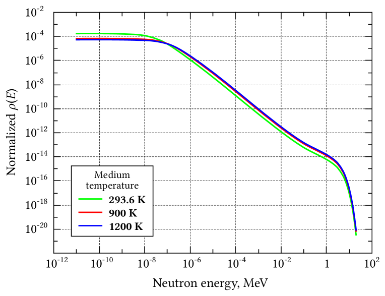
Figure 3: The neutron spectrum (0 - 5 MeV) calculated by the expression (80) for the source of fission neutrons given by the expression (81) for ²³⁵U, and the moderator temperature of 1000 K.

With the decrease of neutron energy ($10~{}eV\leqslant E_{n}\leqslant 100~{}keV$) both terms in the curly brackets of the numerator in the expression (80) become comparable, and therefore this part of the energy spectrum of the moderating neutron may be called a ”transition region”, because it is formed by the contributions of the two terms of the numerator in the expression (80) – i.e. the sum of the fission spectrum and the Fermi spectrum ($\sim 1/E_{n}$). Please note that this part of the moderating neutron spectrum is erroneously marked as the Fermi spectrum in the theoretical scheme shown in Fig. 4.

With further decrease of neutron energy ($E_{n}\leqslant 10~{}eV$) the first term in the curly brackets of the numerator of (80) will be significantly greater than the second one, and effectively determines the energy spectrum of the moderating neutrons in this energy range. However, due to the term $\frac{3}{2}kT$ in the numerator of (80), a neutron energy range of $\frac{3}{2}kT\ll E_{n}\leqslant 10~{}eV$ may be singled out – the energy spectrum of the moderating neutrons will coincide with the Fermi spectrum ($\sim 1/E_{n}$). This is confirmed by the results of the calculations presented in Fig. 3 ($0.03~{}eV\ll E_{n}\leqslant 10~{}eV$). Let us note that Fig. 4 shows the Fermi spectrum ($\sim 1/E_{n}$) up to a certain energy $E_{threshold}$, below which the moderating neutron spectrum is given by the Maxwell spectrum. The form of latter is defined by the temperature of the neutron gas, which in its turn is calculated from the empirical formula connecting it with the temperature of moderating medium.

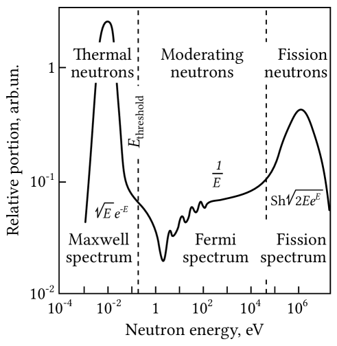
Figure 4: Theoretical scheme of a full energy spectrum of moderating neutrons [8].

With a further decrease of neutron energy we obtain a ”transition” from the Fermi spectrum to the low-energy spectrum near $\sim\frac{3}{2}kT$, and the low-energy part of the moderating neutron spectrum $E_{n}\ll\frac{3}{2}kT$.

According to expression (80), the low-energy part of the neutron spectrum must be constant, since the integral in the numerator of the first term in the curly brackets of (80) almost does not change with the energy decrease. However, it turns out that the microscopic elastic cross-section grows exponentially towards low energies in this range (for example, according to the ENDF/B-VII.0 data and [7], for hydrogen the exponent increases in 1000 times (see. Fig. 5), and for uranium it increases in 100 times). Such behavior of the elastic scattering cross section leads to the appearance of second maximum in the low-energy part of the spectrum. So it is clear that the nature of this maximum is associated with the moderation process of the non-equilibrium system of neutrons (emitted by an isotropic source) on the thermalized system of the moderating medium nuclei. Thus, it cannot be explained by a thermally equilibrium part of the neutron system only, i.e. by Maxwell distribution.

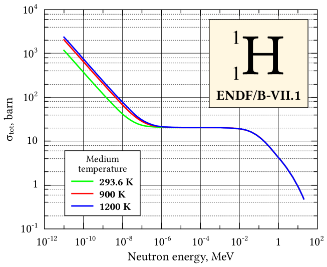
Figure 5: Dependence of microscopic cross-section of the neutron elastic scattering on hydrogen on the neutron energy (from the ENDF/B-VII.1 database).

In contrast to the above considerations, the analogous solution given in [4, 5, 6] was obtained for the traditional scattering law, and the low-energy part of the spectrum has the form of the Fermi spectrum ($\sim 1/E_{n}$). Consequently, it goes to infinity with the neutron energy tending to zero, i.e. there is no low-energy maximum. Therefore, in order to somehow fit the experimental data in the framework of the traditional theory of neutron moderation, the Fermi spectrum ($\sim 1/E_{n}$) is used to a certain boundary energy, below which the moderating neutrons spectrum is given by the Maxwell spectrum, the form of which is defined by the temperature of the neutron gas calculated by the empirical relation to the temperature of the fissile medium (see Introduction).

5 Neutron moderation in non-absorbing media with mass number $A>1$

According to the neutron scattering law (43), which takes into account the thermal motion of the moderating medium nuclei, the moderation law in non-absorbing media with mass number $A>1$ is

$$P(E_{1})dE_{1}=\frac{dE_{1}}{\left[E_{10}^{(L)}+\frac{1}{A}\cdot\frac{3}{2}kT\right](1-\alpha)}$$ (82)

For the moderation law (82) performing the calculations similar to those in [4, 5, 6], we find the following expression for the moderating neutrons flux density:

$$\Phi(E)=\frac{\int\limits_{E}^{\infty}Q(E^{\prime})dE^{\prime}}{\left[E+\frac{1}{A}\cdot\frac{3}{2}kT\right]\Sigma_{s}(E)\xi}+\frac{Q(E)}{\Sigma_{s}(E)},$$ (83)

where $Q(E)$ is the number of generated neutrons with an energy $E$ per unit volume per unit time (see Section 3 above), $\xi$ is the mean logarithmic energy decrement.

By analogy to the standard theory of neutrons moderation, e.g. [4, 5, 6], for the mean logarithmic energy decrement $\xi$ we introduce the following expression (assuming $E_{1}\neq 0$ and $E_{0}\neq 0$):

$$\xi=\left\langle\ln{\frac{E_{0}}{E_{1}}}\right\rangle=\frac{\int\limits_{\alpha\left(E_{0}+\frac{1}{A}\frac{3}{2}kT\right)}^{\left(E_{0}+\frac{1}{A}\frac{3}{2}kT\right)}\ln{\frac{E_{0}}{E_{1}}}P(E_{1})dE_{1}}{\int\limits_{\alpha\left(E_{0}+\frac{1}{A}\frac{3}{2}kT\right)}^{\left(E_{0}+\frac{1}{A}\frac{3}{2}kT\right)}P(E_{1})dE_{1}}=\int\limits_{\alpha\left(E_{0}+\frac{1}{A}\frac{3}{2}kT\right)}^{\left(E_{0}+\frac{1}{A}\frac{3}{2}kT\right)}\ln{\frac{E_{0}}{E_{1}}}\frac{dE_{1}}{\left(E_{0}+\frac{1}{A}\frac{3}{2}kT\right)(1-\alpha)}$$ (84)

Let us perform the variable substitution $E_{1}\Leftrightarrow x$ using the relation

$$E_{0}+\frac{1}{A}\cdot\frac{3}{2}kT=\frac{E_{1}}{x}~{}~{}(x\neq 0),$$ (85)

which implies the following relations

$$E_{0}=\frac{E_{1}}{x}-\frac{1}{A}\frac{3}{2}kT,~{}~{}~{}E_{1}=x\left(E_{0}+\frac{1}{A}\cdot\frac{3}{2}kT\right),$$

$$x=\frac{E_{1}}{E_{0}+\frac{1}{A}\frac{3}{2}kT},~{}~{}~{}dx=\frac{dE_{1}}{E_{0}+\frac{1}{A}\frac{3}{2}kT},$$

from which for (84) we obtain:

$$\xi =\int\limits_{\alpha}^{1}\ln{\left(\frac{\frac{E_{1}}{x}-\frac{1}{A}\frac{3}{2}kT}{E_{1}}\right)}\frac{dx}{(1-\alpha)}=\frac{1}{(1-\alpha)}\int\limits_{\alpha}^{1}\ln{\left(\frac{1}{x}-\frac{1}{E_{1}}\frac{1}{A}\frac{3}{2}kT\right)}dx=$$

$$=\frac{1}{(1-\alpha)}\int\limits_{\alpha}^{1}\ln{\left(\frac{1}{x}-\frac{1}{x\left(E_{0}+\frac{1}{A}\frac{3}{2}kT\right)}\frac{1}{A}\frac{3}{2}kT\right)}dx=$$

$$=\frac{1}{(1-\alpha)}\int\limits_{\alpha}^{1}\ln{\left(\frac{1}{x}\cdot\frac{E_{0}}{E_{0}+\frac{1}{A}\frac{3}{2}kT}\right)}dx=$$

$$=\frac{1}{(1-\alpha)}\left[\int\limits_{\alpha}^{1}\ln{\frac{1}{x}}dx+\ln{\frac{E_{0}}{E_{0}+\frac{1}{A}\frac{3}{2}kT}}\int\limits_{\alpha}^{1}dx\right]=$$

$$=\frac{1}{(1-\alpha)}\int\limits_{\alpha}^{1}\ln{\frac{1}{x}}dx+\frac{1}{(1-\alpha)}\ln{\frac{E_{0}}{E_{0}+\frac{1}{A}\frac{3}{2}kT}}\left(1-\alpha\right)=$$

$$=\frac{1}{(1-\alpha)}\int\limits_{1}^{\alpha}\ln{x}dx+\ln{\frac{E_{0}}{E_{0}+\frac{1}{A}\frac{3}{2}kT}}.$$ (86)

Integrating by parts, we find that the integral in the expression (86):

$$\int\limits_{1}^{\alpha}\ln{x}dx =x\ln{x}|_{1}^{\alpha}-x|_{1}^{\alpha}=\alpha\ln{\alpha}+\left(1-\alpha\right).$$ (87)

Substituting (87) into (86) we obtain the final expression for $\xi$:

$$\xi=\frac{\alpha}{1-\alpha}\ln{\alpha}+1+\ln{\left(\frac{E_{0}}{E_{0}+\frac{1}{A}\frac{3}{2}kT}\right)}.$$ (88)

Thus, in the framework of the new moderation theory we obtain the expression (88) for $\xi$, according to which $\xi$ depends on the initial energy of moderating neutrons $E_{0}$ and the moderating medium temperature $T$. The dependence of the logarithmic energy decrement, calculated by (88), is shown in Fig. 6.

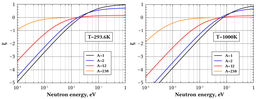
Figure 6: Dependence of the logarithmic energy decrement on the neutron energy, calculated by (88).

However, the expression (88) for $E_{0}\gg\frac{1}{A}\cdot\frac{3}{2}kT$ turns into expression for $\xi$ obtained in the framework of the standard moderation theory, e.g. [4, 5, 6]:

$$\xi\approx 1+\frac{\alpha}{1-\alpha}\ln{\alpha}=1+\frac{(A-1)^{2}}{2A}\ln{\frac{A-1}{A+1}}.$$ (89)

The approximate value of $\xi$ for heavy nuclei is

$$\xi\approx\frac{2}{A+\frac{2}{3}}.$$ (90)

According to the obtained expression (88), for $E_{0}\ll\frac{1}{A}\cdot\frac{3}{2}kT$ the mean logarithmic energy decrement tends to zero with energy decrease, crosses zero, becoming negative and tending further towards $-\infty$ (see Fig. 6). The negative values of $\xi$ correspond to the interactions of the neutrons with the medium nuclei, in which neutrons gain additional energy. Such processes are not considered by the standard moderation theory. It also means that one should use $|\xi|$ instead of $\xi$ in the expression for the neutron flux density (83), and take into account the zero crossing in the calculations.

For the neutron flux density (83), as the neutron flux density $\Phi(E)$ and the neutron density $n(E)$ are connected by (79) [4, 5, 6], we find that the probability density function of the moderating neutrons energy distribution is given by the following expression:

$$\rho(E)=\frac{n(E)}{\int\limits_{0}^{\infty}n(E^{\prime})dE^{\prime}}=\frac{\frac{1}{\sqrt{2E/m_{n}}}\left\{\frac{\int\limits_{E}^{\infty}Q(E^{\prime})dE^{\prime}}{\left[E+\frac{3}{2}kT\right]\Sigma_{s}(E)\xi}+\frac{Q(E)}{\Sigma_{s}(E)}\right\}}{\int\limits_{0}^{\infty}\left[\frac{1}{\sqrt{2E^{\prime}/m_{n}}}\left\{\frac{\int\limits_{E^{\prime}}^{\infty}Q(E^{\prime\prime})dE^{\prime\prime}}{\left[E^{\prime}+\frac{3}{2}kT\right]\Sigma_{s}(E^{\prime})\xi}+\frac{Q(E^{\prime})}{\Sigma_{s}(E^{\prime})}\right\}\right]dE^{\prime}}.$$ (91)

$Q(E)$ is given by the fission spectrum of a fissile nuclide (see Section 3 above).

6 Neutron moderation in non-absorbing moderating media containing several sorts of nuclides

In this case the neutron scattering law is also given by (82). Carrying out the calculations similar to those in [4, 5, 6], we find the following expression for the moderating neutrons flux density:

$$\Phi(E)=\frac{\int\limits_{E}^{\infty}Q(E^{\prime})dE^{\prime}}{\left[E+\frac{1}{A}\cdot\frac{3}{2}kT\right]\Sigma_{s}(E)\bar{\xi}}+\frac{Q(E)}{\Sigma_{s}(E)},$$ (92)

where $Q(E)$ is the number of generated neutrons with energy $E$ per unit volume per unit time (see Section 3 above), $\bar{\xi}$ is the mean logarithmic energy decrement averaged over all sorts of nuclei in the moderating medium [4, 5, 6]:

$$\bar{\xi}=\frac{\sum\limits_{i=1}^{N}\Sigma_{si}\xi_{i}}{\sum\limits_{i=1}^{N}\Sigma_{si}}=\frac{\sum\limits_{i=1}^{N}\Sigma_{si}\xi_{i}}{\Sigma_{s}}$$ (93)

Similarly to the above, the probability density function of the moderating neutrons energy distribution is:

$$\rho(E)=\frac{n(E)}{\int\limits_{0}^{\infty}n(E^{\prime})dE^{\prime}}=\frac{\frac{1}{\sqrt{2E/m_{n}}}\left\{\frac{\int\limits_{E}^{\infty}Q(E^{\prime})dE^{\prime}}{\left[E+\frac{3}{2}kT\right]\Sigma_{s}(E)\bar{\xi}}+\frac{Q(E)}{\Sigma_{s}(E)}\right\}}{\int\limits_{0}^{\infty}\left[\frac{1}{\sqrt{2E^{\prime}/m_{n}}}\left\{\frac{\int\limits_{E^{\prime}}^{\infty}Q(E^{\prime\prime})dE^{\prime\prime}}{\left[E^{\prime}+\frac{3}{2}kT\right]\Sigma_{s}(E^{\prime})\bar{\xi}}+\frac{Q(E^{\prime})}{\Sigma_{s}(E^{\prime})}\right\}\right]dE^{\prime}}.$$ (94)

7 Neutron moderation in absorbing moderating media containing several sorts of nuclides

In this case, the neutron scattering law is also given by (82). Performing the calculations similar to those in [4, 5, 6, 19], we find the following expression for the moderating neutrons flux density:

$$\Phi(E)=\left\{\frac{\int\limits_{E}^{\infty}Q(E^{\prime})dE^{\prime}}{\left[E+\frac{1}{A}\frac{3}{2}kT\right]\Sigma_{t}(E)\bar{\xi}}+\frac{Q(E)}{\Sigma_{t}(E)}\right\}\cdot\exp\left\{-\int\limits_{E}^{\infty}\frac{\Sigma_{a}(E^{\prime})dE^{\prime}}{\left[E^{\prime}+\frac{1}{A}\frac{3}{2}kT\right]\Sigma_{t}(E^{\prime})\bar{\xi}}\right\},$$ (95)

where $\Sigma_{si}$ is the macroscopic scattering cross-section for the $i^{\text{th}}$ nuclide, $\Sigma_{t}=\sum\limits_{i}\Sigma_{s}^{i}+\Sigma_{a}^{i}$ is the total macroscopic cross-section of the fissile material, $\Sigma_{s}=\sum\limits_{i}\Sigma_{s}^{i}$ is the total macroscopic scattering cross-section of the fissile medium, $\Sigma_{a}$ is the macroscopic absorption cross-section.

The Eq. (95) contains the expression for the probability function for the neutrons to avoid the resonance absorption, which now also contains the moderating medium temperature, in contrast to the standard moderation theory [4, 5, 6, 28]:

$$\varphi(E)=\exp\left\{-\int\limits_{E}^{\infty}\frac{\Sigma_{a}(E^{\prime})dE^{\prime}}{\left[E^{\prime}+\frac{1}{A}\cdot\frac{3}{2}kT\right]\Sigma_{t}(E^{\prime})\bar{\xi}}\right\},$$ (96)

Similarly to the above, the probability density function of the moderating neutrons energy distribution is:

$$\rho(E)=\frac{n(E)}{\int\limits_{0}^{\infty}n(E^{\prime})dE^{\prime}}=\frac{\frac{1}{\sqrt{2E/m_{n}}}\left\{\frac{\int\limits_{E}^{\infty}Q(E^{\prime})dE^{\prime}}{\left[E+\frac{3}{2}kT\right]\Sigma_{t}(E)\bar{\xi}}+\frac{Q(E)}{\Sigma_{t}(E)}\right\}\cdot\varphi(E)}{\int\limits_{0}^{\infty}\left[\frac{1}{\sqrt{2E^{\prime}/m_{n}}}\left\{\frac{\int\limits_{E^{\prime}}^{\infty}Q(E^{\prime\prime})dE^{\prime\prime}}{\left[E^{\prime}+\frac{3}{2}kT\right]\Sigma_{t}(E^{\prime})\bar{\xi}}+\frac{Q(E^{\prime})}{\Sigma_{t}(E^{\prime})}\right\}\cdot\varphi(E^{\prime})\right]dE^{\prime}}.$$ (97)

Analyzing the energy spectrum represented by (97), together with its comparison to the complete scheme of the moderating neutrons spectrum rarely found in literature [8], shows that the moderating neutrons spectrum may be described adequately by a single expression, taking into account the moderator temperature.

Let us emphasize that in Section 4 we omitted the consideration of the resonance neutron absorption function (96) during the analysis of the expressions for the flux density and spectrum of the moderating neutrons, because we considered a non-absorbing moderator. This function will affect the ratio of the amplitudes of two maxima in the moderating neutrons flux density and spectrum. It will also reveal a fine resonant structure of the moderating neutron spectrum in the regions of resonance energies (similar to those shown in Fig. 4 from [8]).

8 Conclusion

We obtained the analytical expression for the neutron scattering law for an isotropic source of neutrons, which includes a temperature of the moderating medium as a parameter in general case. The analytical expressions for the neutron flux density and the spectrum of moderating neutrons, also depending on the medium temperature were obtained as well.

As an example of the correct description of the moderating neutron spectrum by the obtained analytical expressions, we present the calculated total energy spectra (from 0 to 5 MeV) of neutrons moderated by the hydrogen medium at temperatures of 1000 K. The fission energy spectrum of neutrons was used for an isotropic neutron source. The calculated spectra are in good agreement with the available experimental data and theoretical concepts of the neutron moderation theory.

The obtained expressions for the moderating neutrons spectra create space for the new interpretations of the physical nature of the processes that determine the form of the neutron spectrum in the thermal region. We found the impact of the elastic scattering cross-sections behavior on the formation of the low-energy maximum in the moderating neutron spectrum It is clear that the nature of this maximum is associated with the process of the non-equilibrium neutron system (generated by an isotropic neutron source) moderation by a thermalized system of moderator nuclei. Therefore it cannot be explained by the thermalized part of the neutron system only, and thus by the Maxwell distribution.

In conclusion it may be noted that the substantially different behavior of the elastic scattering cross-sections for different moderating media (see e.g. ENDF/B-VII.0 or [7]) opens the possibility for the experimental studies of these cross-sections impact on the formation of the low-energy maximum in the moderating neutron spectrum, as well as for the experimental verification of the described analytical expressions.

References

- Weinberg and Wigner [1958] A. M. Weinberg and E. P. Wigner. The Physical Theory of Neutron Chain Reactors. The University of Chicago Press, 1958.
- Akhiezer and Pomeranchuk [2002] A.I. Akhiezer and I.Ya. Pomeranchuk. Introduction into the theory of neutron multiplication systems (reactors). IzdAT, Moscow, 2002. in Russian.
- Galanin [1960] A.D. Galanin. Thermal reactor theory. Pergamon Press, New York, 1960.
- Feinberg et al. [1978] S. M. Feinberg, S.B. Shikhov, and V.B. Troyanskii. The theory of nuclear reactors, Volume 1, Elementary theory of reactors. Atomizdat, Moscow, 1978. in Russian.
- Bartolomey et al. [1989] G.G. Bartolomey, G.A. Bat’, V.D. Baibakov, and M.S. Altukhov. Basic theory and methods of nuclear power installation calculations. Energoatomizdat, Moscow, 1989. in Russian.
- Shirokov [1998] S.V. Shirokov. The nuclear reactor physics. Naukova Dumka, Kiev, 1998. in Russian.
- Stacey [2001] W.M. Stacey. Nuclear Reactor Physics. Wiley-VCH, 2001.
- Vladimirov [1986] V.I. Vladimirov. Practical problems of nuclear reactor operation. Energoatomizdat, Moscow, 1986. in Russian.
- Verkhivker and Kravchenko [2008] G.P. Verkhivker and V.P. Kravchenko. Bases for calculation and design of nuclear power reactors. TEC Publishing, Odessa, 2008. in Russian.
- Rusov et al. [2011a] Vitaliy D. Rusov, Elena P. Linnik, Victor A. Tarasov, Tatiana N. Zelentsova, Igor V. Sharph, Vladimir N. Vaschenko, Sergey I. Kosenko, Margarita E. Beglaryan, Sergey A. Chernezhenko, Pavel A. Molchinikolov, Sergey I. Saulenko, and Olga A. Byegunova. Traveling wave reactor and condition of existence of nuclear burning soliton-like wave in neutron-multiplying media. Energies, 4(9):1337, 2011a. ISSN 1996-1073. doi: 10.3390/en4091337. URL http://www.mdpi.com/1996-1073/4/9/1337.
- Rusov et al. [2011b] V.D. Rusov, V.A. Tarasov, and S.A. Chernezhenko. The modes with the sharpening in the uranium-plutonium fission environment of the technical nuclear reactors and georeactor. Problems of Atomic Science and Technology, 97(2):123–131, 2011b. in Russian.
- Rusov et al. [2013a] V. D. Rusov, V. A. Tarasov, V. M. Vaschenko, E. P. Linnik, T. N. Zelentsova, M. E. Beglaryan, S. A. Chernegenko, S. I. Kosenko, P. A. Molchinikolov, V. P. Smolyar, and E. V. Grechan. Fukushima plutonium effect and blow-up regimes in neutron-multiplying media. World Journal of Nuclear Science and Technology, 3(2A):9–18, 2013a. doi: 10.4236/wjnst.2013.32A002. arXiv:1209.0648v1.
- Rusov et al. [2013b] V.D. Rusov, D.A. Litvinov, E.P. Linnik, V.M. Vaschenko, T.N. Zelentsova, M.E. Beglaryan, V.A. Tarasov, S.A. Chernegenko, V.P. Smolyar, P.A. Molchinikolov, K.K. Merkotan, and P. Kavatskyy. Kamland-experiment and soliton-like nuclear georeactor. part 1. comparison of theory with experiment. Journal of Modern Physics, 4(4):528–550, 2013b. doi: 10.4236/jmp.2013.44075.
- Rusov et al. [2010] V.D. Rusov, V.A. Tarasov, S.A. Chernegenko, and T.L. Borikov. Blow-up modes in uranium-plutonium fissile medium in technical nuclear reactors and georeactor. In Proc. Int. Conf. ”Problems of physics of high energy densities. XII Khariton Topical Scientific Readings”, pages 94–102, Sarov, 2010. Publishing ”RFNC-VNIIEF”. in Russian.
- Prigogine [1968] I. Prigogine. Introduction to Thermodynamics of Irreversible Processes. John Wiley & Sons, New York, 1968.
- Bakhareva [1976] I.F. Bakhareva. Nonlinear nonequilibrium thermodynamics. Saratov University Publishing, 1976. in Russian.
- Kvasnikov [2003] I.A. Kvasnikov. Thermodynamics and statistical physics. Vol.3 ”Theory of nonequilibrium systems”. Editorial URSS, 2003. in Russian.
- Rusov et al. [2015a] V. D. Rusov, V. A. Tarasov, I. V. Sharph, V. N. Vashchenko, E. P. Linnik, T. N. Zelentsova and1 M. E. Beglaryan, S. A. Chernegenko, S. I. Kosenko, and V. P. Smolyar1. On some fundamental peculiarities of the traveling wave reactor. Science and Technology of Nuclear Installations, 2015:703069, 2015a.
- Rusov et al. [2015b] V.D. Rusov, V.A. Tarasov, M.V. Eingorn, S.A. Chernezhenko, A.A. Kakaev, V.M. Vashchenko, and M.E. Beglaryan. Ultraslow wave nuclear burning of uranium-plutonium fissile medium on epithermal neutrons. Progress in Nuclear Energy, 83:105–122, 2015b.
- Kolesov [2006] V. F. Kolesov. Aperiodic pulse reactors. Vol.1. RFNC-VNIIEF Publishing, Sarov, 2006.
- Lukin [2006] Lukin. Physics of the Pulse Nuclear Reactors. RFNC-VNIITF Publishing, Snezhinsk, 2006. in Russian.
- Arapov [2010] Arapov. The results of the physical launch of the br-1m reactor. In Problems of the physics of high energy density. XII Kharitonov thematic scientific readings, pages 22–27, Sarov, 2010. RFNC-VNIIEF Publishing. in Russian.
- Rusov et al. [2007] V. D. Rusov, V. N. Pavlovich, V. N. Vaschenko, V. A. Tarasov, T. N. Zelentsova, V. N. Bolshakov, D. A. Litvinov, S. I. Kosenko, and O. A. Byegunova. Geoantineutrino spectrum and slow nuclear burning on the boundary of the liquid and solid phases of the earth’s core. Journal of Geophysical Research: Solid Earth, 112(B9):n/a–n/a, 2007. ISSN 2156-2202. doi: 10.1029/2005JB004212. URL http://dx.doi.org/10.1029/2005JB004212. B09203.
- Levich et al. [1973] Benjamin G. Levich, V.A. Myamlin, and Yu.A. Vdovin. Theoretical Physics: An Advanced Text Volume 3: Quantum Mechanics. John Wiley & Sons, New York, 1973.
- Levich [1971] V.G Levich. Theoretical Physics: An Advanced Text, Vol. 2: Statistical Physics, Electromagnetic Processes in Matter. Elsevier Science Publishing Co Inc., U.S., 1971.
- Fedorov [1961] N.D. Fedorov. A brief reference book for engineer-physicists. State publishing of literature in the field of nuclear science and technology, Moscow, 1961. in Russian.
- Shirokov and Yudin [1983] Yu. M. Shirokov and N.P. Yudin. Nuclear Physics. Imported Pubn, 1983.
- adn V.A. Tarasov et al. [2012] V.D. Rusov adn V.A. Tarasov, S.I. Kosenko, and S.A. Chernezhenko. The function of resonance absorption probability for the neutron and multiplicate integral. Problems of Atomic Science and Technology, 99(2):68–72, 2012. in Russian.