Gravitational shock wave inside a steadily-accreting spherical charged black hole

Abstract

We numerically investigate the interior of a four-dimensional, spherically symmetric charged black hole accreting neutral null fluid. Previous study by Marolf and Ori suggested that late infalling observers encounter an effective shock wave as they approach the outgoing portion of the inner horizon. Non-linear perturbations could generate an effective gravitational shock wave, which manifests as a drop of the area coordinate $r$ from inner horizon value $r_{-}$ towards zero in an extremely short proper time duration of the infalling observer. We consider three different scenarios: a) A charged black hole accreting a single (ingoing) null fluid; b) a charged black hole perturbed by two null fluids, ingoing and outgoing; c) a charged black hole perturbed by an ingoing null fluid and a self-gravitating scalar field. While we do not observe any evidence for a gravitational shock in the first case, we detect the shock in the other two, using ingoing timelike and null geodesics. The shock width $\Delta\tau$ decreases rapidly with a fairly good match to a new, generalized exponential law, $\Delta\tau\sim e^{-\intop\kappa_{-}(\widetilde{V}_{f})d\widetilde{V}_{f}}$, where $\widetilde{V}_{f}$ is a specific timing parameter for the ingoing timelike geodesics and $\kappa_{-}(\widetilde{V}_{f})$ is a generalized (Reissner-Nordström like) surface gravity of the charged black hole at the inner horizon. We also gain new insight into the inner (classical) structure of a charged black hole perturbed by two null fluids, including strong evidence for the existence of a spacelike $r=0$ singularity. We use a finite-difference numerical code with double-null coordinates combined with an adaptive gauge method in order to solve the field equations from the region outside the black hole down to the vicinity of the $r=0$ singularity.

Department of Physics,

Technion - Israel Institute of Technology,

Haifa 3200003, Israel

1 INTRODUCTION

1.1 Background

The study of the inner structure of classical black holes (BHs) has been an enduring research field in the last couple of decades. Two classes of models were of a particular interest; perturbations on a charged BH background [1, 2, 3, 4, 5, 6, 7, 8, 9, 10, 11, 12, 13, 14, 15, 16, 17, 18] and perturbations on a spinning BH background [19, 20, 21, 22, 23, 24, 25, 26]. The research considered the effects of perturbations on the BH geometry and the differences from the corresponding non-perturbed geometries, the Reissner-Nordström (RN) geometry in the charged case and the Kerr geometry in the spinning case. Both classes of models share a similar horizon structure (of an (outer) event horizon (EH) and an inner horizon (IH)); while the perturbed spinning class is believed to be closely related to realistic astrophysical BHs, the perturbed charged class (usually) offers a simpler analysis due to spherical symmetry. RN geometry has a well known $r=0$ timelike singularity; Kerr geometry has a timelike $r=0$ ring singularity. The study of the perturbed geometries focused specifically on the development of additional singularities inside the BHs.

The IH of RN and Kerr geometries also operates as Cauchy Horizon (CH), a null hypersurface that marks the boundary of physical predictability. Penrose pointed out that this hypersurface is a locus of infinite blueshift in both geometries; [1] he predicted it should develop curvature singularity in the presence of perturbations. Hiscock confirmed this prediction with analytical analysis of an ingoing null fluid perturbation. [4] Hiscock used the Reissner-Nordström-Vaidya (RNV) model, [27] representing a neutral null fluid — a stream of massless particles — flowing on a charged black hole background. This model has two variants, ingoing and outgoing, distinguished by the null direction of the fluid; Hiscock used the ingoing variant. He discovered that a nonscalar curvature singularity develops at the ingoing section of the IH (which is CH in this scenario). Some time later, Poisson and Israel have diagnosed the development of a singularity at the CH of a different model, the mass inflation model; [6, 7] this model includes two null fluids, ingoing and outgoing, flowing on a charged BH background. In this case, however, the singularity is scalar and there is a divergence of the mass function at the vicinity of the singular CH. Despite of this, Ori has later proved that this null singularity is deformationally weak [8] in the Tipler sense ([28], see also Ref. [29]); the metric tensor components approach a finite value on the CH and an infalling observer only experiences finite tidal distortion at the crossing of the CH. During the 1990’s, numerical investigations of self-gravitating scalar field perturbations on a charged background [10, 12] suggested that in this case the singular CH is a subject to a process of “focusing”; the area coordinate $r$ monotonically decreases along CH up to the point where it vanishes and the singularity becomes spacelike. The analysis of perturbations on a spinning background revealed a similar general picture; [19, 20, 21, 22, 26] in this case too, a weak null curvature singularity develops at the CH.

1.2 Shock wave at the inner horizon

Marolf and Ori (MO) have recently demonstrated analytically the existence of additional null (effective) singularity at the outgoing portion of the IH, an effective shock wave singularity. [30] An infalling observer experiences a finite (effective) jump in the values of various perturbation fields across the IH at late times. This change actually occurs on a finite proper time duration $\Delta\tau$; however, this duration decreases exponentially with infall time and becomes unresolvable for an observer of given sophistication. The observer may experience a metric discontinuity if the perturbation is nonlinear; this metric discontinuity, or gravitational shock, manifests as an (effective) sheer drop in the value of the area coordinate $r$ (where $g_{\theta\theta}=r^{2}$).

MO have considered specifically a wide variety of test perturbations (scalar field, electromagnetic and gravitational perturbations) on RN and Kerr backgrounds and non-linear scalar field perturbation on a spherical charged background. They estimated that their arguments should be relevant to non-linear perturbations on a spinning BH background as well but did not include a full analysis of such case. Their scenarios were asymptotically flat and asymptotically static; they relied upon known properties of RN and Kerr geometries. MO argued that the shock wave singularity is “stronger” and more violent than the CH singularity; an infalling observer experiences integrated deformation across the IH which does not decrease with infall time, but remains fixed and of order unity.

More recently, Eilon and Ori (EO) have confirmed numerically the existence of the shock wave. [31] EO considered two different scenarios, the evolution of a test scalar-field on RN background and the evolution of a self-gravitating scalar-field on a dynamical charged BH background. They have demonstrated the existence of the shock in the scalar field $\Phi(\tau)$ in both cases, and in $r(\tau)$ in the self-gravitating case. EO also confirmed MO’s prediction about the exponential decrease in $\Delta\tau$ (the exponential sharpening rate) of the shock; they have defined characteristic $\Delta\tau$ widths for both $\Phi(\tau)$ and $r(\tau)$ and showed that they decrease exponentially with infall time. Although most of their analysis was based on timelike geodesics, EO were the first to exhibit the shock on null geodesics; they displayed the gravitational shock in $r(\lambda)$ (where $\lambda$ is the affine parameter) on a three-dimensional graph using a dense set of null geodesic. The geodesics’ sheer drop in $r$ at the IH created a vertical wall-like structure; they argued that this may be the clearest visual presentation of the shock.

Fig. 1 illustrates the gravitational shock scenario considered by EO through the relevant Penrose diagram. The inner (classical) structure of the BH in this case is well known (with the possible exception of the shock wave), and includes a strong spacelike $r=0$ singularity and a weak null singularity at the CH. The shock is located at the outgoing IH of the BH at late times (the solid green line). The full blue curve and the dashed blue line represent a late timelike geodesic and a late null geodesic, accordingly; both cross the IH and reach the spacelike $r=0$ singularity. Due to the gravitational shock, the journey from the IH ($r=r_{-})$ to $r=0$ takes an extremely short proper time duration $\Delta\tau$ (or an affine parameter interval $\Delta\lambda$). Fig. 1 describes the case of a self gravitating scalar field perturbation on an eternal RN background. However, EO shock results could be also attributed to the case of a spherical charged collapse; they could describe the dynamics outside a collapsing charged shell or star. The shock wave phenomenum, as argued by MO and EO, is a general phenomenum of perturbed charged or spinning BHs; it is not limited to the eternal RN (or Kerr) scenarios.

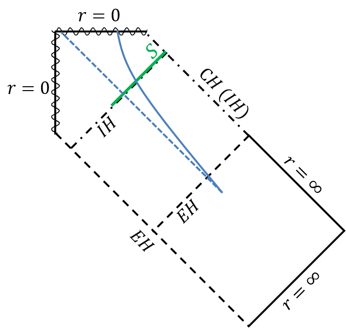
Figure 1: Penrose diagram of a charged BH perturbed by a self gravitating scalar field. Solid black diagonal lines denote null infinity; dashed black diagonal lines denote the event horizon (EH). Dashed-dotted line denotes the inner horizon (IH); the ingoing IH functions as a Cauchy horizon (CH). Wavy lines denote the timelike $r=0$ singularity of the initial RN spacetime and the spacelike $r=0$ singularity of the perturbed spacetime. An effective gravitational shock wave develops along the solid green line denoted “S” (at the outgoing IH). The full blue line represents a typical timelike geodesic that crosses the shock; the dashed blue line is a typical null geodesic. The shock manifests as a sharp drop in the values of the area coordinate $r$ along both geodesics, from $r_{-}$ to zero, in an extremely short proper time duration $\Delta\tau$ (timelike geodesic) or an affine parameter interval $\Delta\lambda$ (null geodesic).

EO considered a single type of perturbation, a neutral massless scalar-field. They also considered a relatively simple scenario, asymptotically flat BH accreting a single scalar field pulse that decays at late times. However, as Hamilton and Avelino has pointed out, [32] realistic astrophysical BHs steadily accrete dust and cosmic microwave background (CMB) photons on cosmological timescales. We wish to extend EO research to a more realistic accretion scenario, and to a different type of perturbation, a neutral null-fluid, which could represent (up to some extent) CMB photons. Due to scope limitations, we focus our analysis on the gravitational shock, the shock in the area coordinate $r$. We consider in the current paper three different physical scenarios; all three include long term accretion of a null-fluid stream by a charged BH. In the first scenario, the ingoing null-fluid stream is the only perturbation; we do not detect a gravitational shock in this case. In the second and third scenarios we add an outgoing null-fluid pulse and a self-gravitating scalar-field pulse (accordingly) to the ingoing null-fluid stream. We detect a gravitational shock wave in both scenarios, and uncover different behaviour of the shock due to the accretion of the null-fluid stream. The sharpening rate of the shock differs from EO (and MO) result — our shock sharpens more rapidly, with a fairly good match to a generalized exponential sharpening rate law. MO and EO used (mostly) timelike geodesics in their shock analysis, though EO had some results taken from null geodesic. We employ both timelike and null geodesics, alternately, throughout our entire analysis. In the course of our shock exploration we uncover two interesting results on the inner (classical) structure of a charged BH perturbed by two null fluids — a strong evidence for the existence of a spacelike $r=0$ singularity and a possible, uncertain indication to the presence of a null, non-naked, $r=0$ singularity.

The motivation for our third scenario, a mixed null-fluid/scalar field perturbation, requires a further explanation. The dynamics of scalar field perturbation are different from those of null fluid perturbation and more interesting in the sense that they are more similar to those of realistic gravitational or electromagnetic perturbations. EO have already demonstrated the presence of a shock in the case of self gravitating scalar field perturbation; here we are interested in observing the effect of the null fluid stream on a previously generated shock. This scenario also allows a better comparison of our shock results with EO results than the two null fluids case, as the mixed scenario is basically EO’s scenario with the addition of an ingoing null fluid stream. Lastly, the mixed scenario is a “toy model” for an astrophysical BH accreting both dust (simulated by the scalar field) and radiation (simulated by the null fluid).

The paper has the following structure: The problem is formulated in terms of unknown functions, field equations, and initial data setup in Sec. 2. The description in this section is mostly general and applies for all three scenarios, which are distinguished from each other by initial data setup. We sketch this separation schematically in Sec. 2; the details are described in Secs. 4-6. The numerical algorithm is discussed in Sec. 3; we describe in this section the numerical solver of the field equations and outline additional important calculations and the presentation of numerical results. Since the field equations and the numerical algorithm were discussed extensively in a previous paper [33] and are quite similar to those used by EO, we only describe them briefly here, focusing on the differences from EO setup. We then analyze the case of a single ingoing null-fluid stream on a charged background in Sec. 4. In particular, we exhibit the lack of evidence for gravitational shock. The case of two null fluids (ingoing and outgoing) on a charged background is analyzed in Sec. 5, where we demonstrate the existence of a gravitational shock wave and analyze the rate of shock sharpening. We do the same for the third case, an ingoing null-fluid stream with a self-gravitating scalar-field pulse on a charged background, in Sec. 6. We summarize and discuss our results in Sec. 7.

2 FIELD EQUATIONS

We consider in this paper three different physical scenarios: (i) a preexisting RN BH accreting a single (ingoing) null-fluid; (ii) two null fluids, ingoing and outgoing, flowing on a charged BH background; (iii) a preexisting RN BH accreting a a single (ingoing) self-gravitating scalar-field pulse and a single (ingoing) null-fluid. We investigate these cases using the same set of field equations solved by the same numerical algorithm; they are distinguished by initial conditions choice (see section 2.1).

The null fluid is neutral and minimally coupled. The scalar field is the same self-gravitating scalar field used by EO; it is uncharged, massless and minimally coupled, satisfying the massless Klein-Gordon equation $\Square\Phi=0$. In all three cases the initial RN geometry has mass $M_{0}$ and charge $Q$. The line element in double-null coordinates $(u,v,\theta,\varphi)$ is

$$ds^{2}=-e^{\sigma(u,v)}dudv+r(u,v)^{2}d\Omega^{2}\,,$$ (1)

where $d\Omega^{2}\equiv d\theta^{2}+\sin^{2}\theta\,d\varphi^{2}$. In principle, our three unknown functions are the metric functions $\sigma(u,v)$ and $r(u,v)$ and the scalar field $\Phi(u,v)$, although in the single null fluid and two null fluids cases the scalar field is trivially solved ($\Phi(u,v)=0$).

The field equations are given by $G_{\mu\nu}=8\pi(T_{\mu\nu}^{\Phi}+T_{\mu\nu}^{Q}+T_{\mu\nu}^{NF})$, where $T_{\mu\nu}^{\Phi}$ and $T_{\mu\nu}^{Q}$ are the energy-momentum tensors of the scalar and electromagnetic fields; $T_{\mu\nu}^{NF}$ is the energy-momentum tensor of the null fluid and satisfies (see e.g. Ref. [7])

$$T_{\mu\nu}^{NF}=\rho_{in}k_{\mu}k_{\nu}+\rho_{out}l_{\mu}l_{\nu}\>,$$ (2)

where $\rho_{in},\rho_{out}$ are constants, $k_{\mu}$ a radial null vector pointing inward and $l_{\mu}$ a radial null vector pointing outward. This tensor has only two nonvanishing components in double null coordinates, $T_{vv}^{NF}$ and $T_{uu}^{NF}$. $T_{vv}^{NF}$ corresponds to the first term in Eq. (2), the ingoing null fluid; $T_{uu}^{NF}$ corresponds to the second term, the outgoing null fluid. We henceforth define the null fluid by these components (rather than $\rho_{in},\rho_{out},k_{\mu}$ and $l_{\mu})$ for the sake of simplicity. Overall, our field equations consist of three evolution equations,

$$r,_{uv}=-\frac{r,_{u}r,_{v}}{r}-\frac{e^{\sigma}}{4r}(1-\frac{Q^{2}}{r^{2}})\,,$$ (3)

$$\sigma,_{uv}=\frac{2r,_{u}r,_{v}}{r^{2}}+\frac{e^{\sigma}}{2r^{2}}(1-\frac{2Q^{2}}{r^{2}})-2\Phi,_{u}\Phi_{,v}\,\,,$$ (4)

$$\Phi,_{uv}=-\frac{1}{r}(r,_{u}\Phi,_{v}+r,_{v}\Phi,_{u})\,,$$ (5)

and two constraint equations,

$$r,_{uu}-r,_{u}\sigma,_{u}+r(\Phi,_{u})^{2}+4\pi rT_{uu}^{NF}=0\,,$$ (6)

$$r,_{vv}-r,_{v}\sigma,_{v}+r(\Phi,_{v})^{2}+4\pi rT_{vv}^{NF}=0\,.$$ (7)

The derivation of the field equations is fairly standard and, with the exclusion of the null fluids terms, has been discussed extensively in a previous paper [33] (in Sec. II and the appendix) and in other works. [14] The addition of the null fluid to the model is trivial, however; it contributes a single term for each of the constraint equations (6) and (7) while the evolution equations remain unchanged. The evolution and constraint equations are consistent; the constraint equations need only be imposed at the initial rays. Hence $T_{uu}^{NF}$ and $T_{vv}^{NF}$ do not have “evolution equations”; they are calculated on every point of the grid from the constraint equations.

2.1 Characteristic initial conditions

The characteristic initial hypersurface includes two null rays, $u=u_{0}$ and $v=v_{0}$. We choose four functions on each initial ray, which correspond to two initial conditions for the unknowns $\sigma$ and $\Phi$ and two initial functions for the energy-momentum components $T_{uu}^{NF}$ and $T_{vv}^{NF}$. The function $r$ is determined by a choice of a single parameter — $r(u_{0},v_{0})\equiv r_{0}$ — and numerical solution of the constraint equations — Eq. (6) at $v=v_{0}$ and Eq. (7) at $u=u_{0}$.

The line element (1) implies that initial conditions choice for $\sigma$ is equivalent to a gauge choice for the null coordinates $u$ and $v$. A gauge transformation $v\rightarrow v^{\prime}(v),u\rightarrow u^{\prime}(u)$ does not change $r$ or $\Phi$, but it does change $\sigma$, according to

$$\sigma\rightarrow\sigma^{\prime}=\sigma-\ln(\frac{du^{\prime}}{du})-\ln(\frac{dv^{\prime}}{dv})\,\,.$$ (8)

Our initial conditions choice for $\sigma$ corresponds to the maximal-$\sigma$ gauge, defined by

$$\sigma(u_{0},v)=0\,,\,\>\sigma_{max}(u)=0\,,$$ (9)

where $\sigma_{max}(u)$ is a function which specifies the maximal value of $\sigma$ on each constant $u$ line (at the range $v_{0}\leq v\leq v_{max})$. This adaptive gauge addresses and solves a numerical resolution loss problem, inherent to long-time simulations in double-null coordinates near the EH (see Ref. [33]). The gauge condition $\sigma_{max}(u)=0$ translates to initial condition on $\sigma(u,v_{0})$ via extrapolation procedure, explained in Sec. VII of Ref. [33].

Table 1 outlines the initial functions choice for our scenarios. We focus here at the fundamental differences between the scenarios — which initial functions vanish and which do not — and not on the details of the non-vanishing functions, described later at the relevant sections (4.1, 5.1 and 6.1). Note that $\sigma$ and $T_{vv}^{(NF)}$ have the same basic definition in all three cases.

Function\Scenario	Single null fluid	Two null fluids	Mixed
$\sigma$	$\begin{array}[t]{c}\sigma(u_{0},v)=0\\ \sigma_{max}(u)=0\end{array}$	$\begin{array}[t]{c}\sigma(u_{0},v)=0\\ \sigma_{max}(u)=0\end{array}$	$\begin{array}[t]{c}\sigma(u_{0},v)=0\\ \sigma_{max}(u)=0\end{array}$
$\Phi$	$\begin{array}[t]{c}\Phi(u_{0},v)=0\\ \Phi(u,v_{0})=0\end{array}$	$\begin{array}[t]{c}\Phi(u_{0},v)=0\\ \Phi(u,v_{0})=0\end{array}$	$\begin{array}[t]{c}\Phi(u_{0},v)\neq 0\\ \Phi(u,v_{0})=0\end{array}$
$T_{uu}^{NF}$	$\begin{array}[t]{c}T_{uu}^{NF}(u_{0},v)=0\\ T_{uu}^{NF}(u,v_{0})=0\end{array}$	$\begin{array}[t]{c}T_{uu}^{NF}(u_{0},v)=0\\ T_{uu}^{NF}(u,v_{0})\neq 0\end{array}$	$\begin{array}[t]{c}T_{uu}^{NF}(u_{0},v)=0\\ T_{uu}^{NF}(u,v_{0})=0\end{array}$
$T_{vv}^{NF}$	$\begin{array}[t]{c}T_{vv}^{NF}(u_{0},v)\neq 0\\ T_{vv}^{NF}(u,v_{0})=0\end{array}$	$\begin{array}[t]{c}T_{vv}^{NF}(u_{0},v)\neq 0\\ T_{vv}^{NF}(u,v_{0})=0\end{array}$	$\begin{array}[t]{c}T_{vv}^{NF}(u_{0},v)\neq 0\\ T_{vv}^{NF}(u,v_{0})=0\end{array}$

Table 1: Initial functions choice for the three different physical scenarios considered in this paper. The table outlines the separation between the scenarios by their initial functions choice; it is created by different choices for the energy momentum tensor component of the outgoing null fluid ($T_{uu}^{NF}$) and the scalar field $\Phi$. The table also contains initial functions choice for the energy momentum tensor component of the ingoing null fluid ($T_{vv}^{NF}$) and the metric function $\sigma$. The condition $\sigma_{max}(u)=0$ refers to the maximal-$\sigma$ gauge condition; the maximal value of $\sigma$ on each $u=const.$ grid ray is set to be zero. This condition translates to initial condition on $\sigma(u,v_{0})$ via extrapolation procedure, explained in Sec. VII of Ref. [33].

2.2 Black hole mass and surface gravity

Our shock analysis requires an estimation of the (growing) BH mass during the simulation and its changing surface gravity at the IH. We use the mass function $m(u,v)$ introduced in Ref. [7], which in our coordinates translates to

$$m=(1+4e^{-\sigma}r,_{u}r,_{v})r/2+Q^{2}/2r\,.$$ (10)

We also follow EO ansatz for the event horizon location — the (first) $u$ value where $r,_{v}$, evaluated at the final ingoing ray of the numerical grid $v=v_{max}$, changes its sign from positive to negative. We denote this value as $u_{h}$. We define the black hole mass $m_{BH}(v)$ as the value of the mass function along the event horizon,

$$m_{BH}(v)\equiv m(u_{h},v)\,.$$

This is a monotonically increasing function in our simulation. The values of the EH and IH also changes, according to

$$r_{\pm}(v)=m_{BH}(v)\pm\sqrt{m_{BH}^{2}(v)-Q^{2}}\,,$$ (11)

and they imply a steady change in the BH surface gravity at the EH and IH,

$$\kappa_{\pm}(v)=\frac{\sqrt{m_{BH}^{2}(v)-Q^{2}}}{r_{\pm}^{2}(v)}\,.$$ (12)

We specifically denote the values of the BH mass, EH, IH and surface gravity at last ingoing ray $v=v_{max}$ as $m_{BH,vmax},r_{\pm,vmax}$ and $\kappa_{\pm,vmax}$ accordingly.

The functions $r_{\pm}(v)$ and $\kappa_{\pm}(v)$ could be reexpressed in terms of a different advanced null coordinate $V(v)$ with the appropriate gauge transformation, as we indeed do below.

3 NUMERICAL ALGORITHM

We solve the field equations on a double-null grid; the grid has fixed spacings in $u$ and $v$ (denoted $\Delta u,\Delta v$). We choose $\Delta u=\Delta v=\frac{M_{0}}{N}$, where $M_{0}$ is the initial BH mass and $N$ is assigned several different values on each run (usually $80,160,320,640$), in order to confirm numerical convergence. The numerical solution begins on the initial ray $u=u_{0}$ and progresses towards the final ray $u=u_{max}$; along each $u=const$ ray the solution is advanced from $v=v_{0}$ to $v=v_{max}$. The evolution equations (3-5) are discretized using a standard finite-differences scheme; we also apply a predictor-corrector scheme with second order accuracy, as described in detail in Sec. III of Ref. [33]. The numerical convergence of our unknown functions is usually second order convergence; however, there is a typical decline in performance at the close vicinity of the $r=0$ singularity ($r\sim 0.1$ or less, with some variations) to first order convergence. This effect is (partially) caused by numerical (artificial) fluxes generated by the solution of the constraint equation (6) at the close vicinity of the singularity. In order to avoid these fluxes, we choose $u_{max}$ value such as $r(u,v_{0})$ never falls below $0.1$.

3.1 Geodesics definitions

The previous section described the generation of results on a numerical double-null grid; however, shock analysis requires consideration of results on ingoing geodesics. MO’s original analysis had considered timelike geodesics; EO demonstrated that null geodesics could be effective as well for the exploration of the gravitational shock, although they mainly focused on timelike geodesics. We consider here alternately timelike and null geodesics. Since the derivation of both types has already been described in detail by EO, we give here just a quick summary of geodesics definitions and behaviour, focusing on the differences from EO setup. A full description of the derivation could be found at the appendix of EO.

3.1.1 Timelike geodesics

Timelike geodesics are more “physical” than null geodesics in the sense that they describe the trajectories of actual (test) observers or probes falling into the BH. In our double-null grid, timelike geodesics are a series of bent curves $v(u)$ that typically do not cross grid points. They extend along the entire grid, from the initial ray $u=u_{0}$ up to $u=u_{max}$, unless they encounter $r=0$ (or $v=v_{max}$) before $u=u_{max}$. We derive these curves by solving the geodesic equation and use second order interpolation in order to find the unknown functions on these curves. In addition, we calculate the proper time $\tau$ for each geodesic; we set $\tau=0$ on each geodesic to be the time in which it crosses the EH.

MO and EO considered a family of radial geodesics related to each other by time translation, or a time-translated set of geodesics (TTSG). TTSG are especially useful for gravitational shock analysis since they share the same $r(\tau)$ function up to the location of the shock (if exists). Hence observation of shock formation and development is very simple. Unfortunately, time translation symmetry is a property of static geometries and thus no longer available in our case.

We define our family of timelike geodesics in a similar fashion to EO approximated TTSG in the self-gravitating scalar-field case, using an analogy to the behavior of exact radial TTSG in RN spacetime with energy parameter $E=-u_{t}=1$. For these RN geodesics, $\dot{r}$ satisfies

$$\dot{r}=-\sqrt{E^{2}-(1-\frac{2M}{r}+\frac{Q^{2}}{r^{2}})}\,\,,$$

where $M$ and $Q$ are the mass and charge parameters of RN BH. This relation reduces to $-(2M/r-Q^{2}/r^{2})^{1/2}$ in the case of $E=1$; we replace $M$ with $m(u_{0}v)$, the initial mass parameter at the first point of the geodesic, to obtain

$$\dot{r}(u_{0},v)=-\sqrt{\frac{2m(u_{0},v)}{r(u_{0},v)}-\frac{Q^{2}}{r(u_{0},v)^{2}}}\,\,\,.$$ (13)

Eq. (13) defines our radial timelike geodesic family and supplies the required initial condition for the solution of the geodesic equation. In the self gravitating scalar field case analyzed by EO, this definition reproduces, asymptotically, the behaviour of an exact radial TTSG in RN spacetime. In our case it does not, since our simulation is not asymptotically static. Our geodesic family should not be considered an approximated TTSG by any means, but rather as a family of radial timelike geodesics (weakly) correlated by their initial $\dot{r}$ value.

3.1.2 Null geodesics

Null geodesics are “simpler” than timelike geodesics since in our double-null grid they are just $v=const$ grid rays. We do not need to solve the geodesic equation in order to find their shape; we do not need to interpolate our grid results; we just need to define and calculate an appropriate affine parameter $\lambda$ and associate it to a certain $v=const$ ray in our grid. This “straight line” behavior is also convenient to shock analysis since it allows a clear observation of the gravitational shock in three-dimensional graphs.

The derivation of the affine parameter is described in appendix A2 of EO. The affine parameter $\lambda$ has normalization freedom; we fix this freedom by demanding $\frac{d\lambda}{dr}=-1$ at the EH. We also set $\lambda=0$ to be the EH crossing time on each null geodesic.

3.1.3 Timing parameters

Shock analysis requires the assignation of a timing parameter value for each geodesic, which is particularly important for the analysis of shock sharpening rate. In principle, a timing parameter assignment involves two distinct choices; the choice of an appropriate time coordinate and the choice of a specific point on the geodesic in which the coordinate is evaluated. MO and EO used the same timing parameter for their timelike geodesics, $v_{eh}$, the value of Eddington advanced time coordinate at the EH crossing. Since in our scenarios we do not have a relevant RN (or asymptotically RN) geometry to associate this coordinate with, this choice is no longer an option. Instead, we use timing parameters based on RNV advanced time coordinate. We use two variants of this coordinate, the initial ray RNV advanced time coordinate, denoted $V$, and the event horizon RNV advanced time coordinate, denoted $\widetilde{V}$. Both variants are derived through association with the ingoing RNV metric (Eq. (18)). The derivation of each variant and their interpretation in our different scenarios are described at Sec. A.1 of the appendix.

The association of such timing parameter to null geodesics is pretty straightforward; since they are simply $v=const$ lines, they also have a single value of $V$ or $\widetilde{V}$. The association of timing parameter to timelike geodesics is more complex. We consider in this paper two timing parameters for timelike geodesics, $V_{h}$, which is the value of $V$ at the EH crossing, and $\widetilde{V}_{f}$, which is the last $\widetilde{V}$ value of the geodesic.

3.2 Presentation of numerical results

As we already mentioned above, we have employed several grid refinement levels in our simulation. Most of the numerical results displayed in this paper are based on data from the best resolution, $N=640$. There are two exceptions: (i) The contour graphs of $r(u,v)$ (Figs. 3, 6, and 12) are based on data from $N=640$, but there is a sampling procedure involved in order to avoid memory problems. We specify the sampling rate in $u$ and $v$ ($\Delta_{s}u,\Delta_{s}v$) on the caption of each figure; we have chosen it with care in order to avoid misrepresentation of the results. (ii) The graphs which display data along individual timelike geodesics (Figs. 4(a), 7(a) and 13(a)) also display data from the second best resolution $(N=320)$ in dashed curves (where the $N=640$ data is displayed in solid curves). However, the results from the different resolutions overlap, and the $N=320$ data is indistinguishable. The shifted versions of these graphs (Figs. 7(c) and 13(c)) include just the data from $N=640$.

We use standard general relativistic units in which $c=G=1$, and an additional unit choice which fixes the initial RN mass parameter as $M_{0}=1$. We also set $u_{0}=v_{0}=0$ in the numerics.

4 SINGLE NULL FLUID CASE

We begin our analysis with the simplest case, a preexisting RN BH accreting a single (ingoing) null-fluid. Although we do not observe a gravitational shock in this case, it allows us to establish the descriptions of the ingoing null-fluid stream and the basic shock wave analysis before the study of more complex cases. We first describe the setup of initial data for the initial RN geometry and $T_{vv}^{NF}$; we move on to describe the resultant structure of spacetime and the location of the domain of integration in it; we then demonstrate the lack of evidence for a gravitational shock presence.

4.1 Basic parameters and initial conditions

The initial RN geometry could be described in Schwarzschild coordinates as

$$ds^{2}=-f(r)dt^{2}+f(r)^{-1}dr^{2}+r^{2}d\Omega^{2}\,,$$ (14)

where $f\equiv 1-2M_{0}/r+Q^{2}/r^{2}$. Following EO choice, we choose here an initial mass of $M_{0}=1$ (which is actually a unit choice) and a charge parameter $Q=0.95$.

The ingoing null-fluid stream is defined on the initial ray $u=u_{0}$; it begins at a certain $r$ value on this ray (denoted $r_{1}$) and does not cease up to the maximal grid ray $v=v_{max}$. The stream has the general form

$$T_{vv}^{NF}(u_{0},v)=\begin{cases}\begin{array}[]{c}A_{1}(1-e^{r_{1}-r})^{2}\frac{1}{r^{2}r,_{u}^{2}}\\ 0\end{array}&\begin{array}[]{c}|\,\,\,\,\,\,\,\,\,\,\,\,\,r\geq r_{1}\\ |\,\,otherwise,\end{array}\end{cases}$$ (15)

where $A_{1}$ is an amplitude parameter and $r,r,_{u}$ are functions of $v$ along the initial ray. We have selected this form to emulate the behaviour of a linear null fluid at late times; we have achieved this goal, as demonstrated in Sec. A.2 of the appendix. The factor $(1-e^{r_{1}-r})^{2}$ ensures a smooth (and quick) transition from the null phase to the linear phase. We choose $r_{1}=10$; this value is reached on the initial ray $u=u_{0}$ at $v_{3}\approx 12.54$ (or $V_{3}\approx 5.63$). Although the stream does not cease in our simulation, we assume it ceases at some point in the future, denoted $v=v_{4}$ (or $V=V_{4})$, so that the asymptotic spacetime has RN geometry with a new (and unknown) mass parameter $m_{final}$ and a charge parameter $Q=0.95$. The amplitude $A_{1}$ monitors the mass contribution of the stream; we choose $A_{1}=3.4555203\times 10^{-4}$ which yields a mass of $m_{BH,vmax}=2.5$. This mass fits EH value of $r_{+,vmax}\simeq 4.812$, IH value of $r_{-,vmax}\simeq 0.1875$, and an extreme value of the IH surface gravity at $v=v_{max},$ $\kappa_{-,vmax}$$\simeq 65.8$.

The remaining initial values are taken according to the first column of table 1. In particular, $T_{vv}^{NF}$ vanishes on $v=v_{0}$; the outgoing null fluid $T_{uu}^{NF}$ and the scalar field $\Phi$ vanish on both initial rays $(u=u_{0}$ and $v=v_{0}$); $\sigma$ conforms on both rays with the maximal-$\sigma$ gauge condition (Eq. (9)). $r$ is calculated numerically on both rays from the solution of the constraint equations, Eq. (6) at $v=v_{0}$ and Eq. (7) at $u=u_{0}$.

The domain of integration is $u_{0}=v_{0}=0$, $u_{max}=260.5421875$, and $v_{max}=120$. The value of $r$ in the initial vertex is $r_{0}=5$ and it grows up to $r\simeq 49.47$ at $r(u_{0},v_{max})$. The other two corners of the grid are $r(u_{max},v_{0})\simeq 0.1004$ and $r(u_{max},v_{max})\simeq 0.1868$.

4.2 The structure of spacetime

The location of the numerical grid in spacetime and the structure of spacetime are illustrated in Fig. 2. The outgoing initial ray $u=u_{0}$ is located outside the BH, while the ingoing initial ray $v=v_{0}$ penetrates the BH and passes the outgoing IH. Panel (b) demonstrates that spacetime could be divided into three distinct patches: (i) the initial RN geometry (RN1, at $v<v_{3}$) with mass parameter $M_{0}$ and charge $Q$; (ii) the ingoing null-fluid stream region ($v_{3}\leq v\leq v_{4})$, denoted RNVi; (iii) the final RN Geometry (RN2, at $v>v_{4})$, with mass parameter $m_{final}$ and charge $Q$, which is not covered by our simulation. All three patches of spacetime are extendable; the only “neighboring” singularity is the original timelike $r=0$ singularity of the initial RN geometry. (There are also similar singularities of RNV geometry and the final RN geometry, but they are not drawn in this diagram since they are not in the vicinity of the grid).

This structure is demonstrated by the numerical results of $r(u,v)$, depicted as a contour graph in Fig. 3. Panel (a) describes the entire grid; in particular, one could notice the zone outside the BH as a region in which $r$ values rise with $v$ (at the bottom of the graph, up to $u_{h}\simeq 69.29$). Panel (b) focuses at the vicinity of $u=u_{max}=260.5421875$. This high zoom level (of order of $0.2$ in $u$) demonstrates that the grid ends regularly.

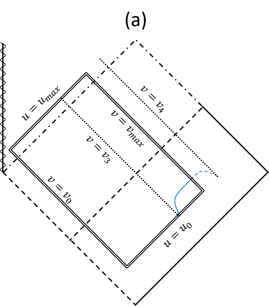
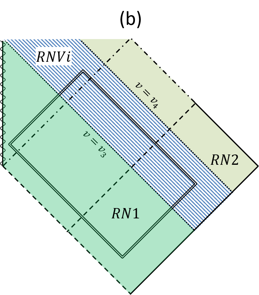
Figure 2: Penrose diagrams illustrating the structure of spacetime in the single null fluid case. Both panels describe the location of the numerical domain of integration and the ingoing null fluid stream in spacetime; while panel (a) focuses on initial data, panel (b) analyzes the different patches of spacetime. In both panels, the domain’s limits are denoted by a double black line; solid black lines denote null infinity; dashed black lines denote the EH; dashed-dotted black lines denote the IH. Wavy vertical lines denote the timelike $r=0$ singularity of RN geometry; dotted black lines denote the ingoing null-fluid stream limits $v=v_{3}$ and $v=v_{4}$. The blue curve in panel (a) represents the ingoing null-fluid stream on the initial ray $u=u_{0}$; its shape roughly describes the stream contribution to the mass function derivative $m,_{V}$. The dashed part of the curve represents the extension of the stream outside the domain of integration up to its termination at $v=v_{4}$. Panel (b) demonstrates that spacetime could be divided into three distinct patches; patches RN1 and RN2 fit the initial RN geometry and the final RN geometry accordingly; they are separated by the ingoing null-fluid stream patch RNVi (diagonal blue stripes).

Figure 3: Numerical results for $r(u,v)$ in the single null fluid case. Both panels display contour graphs of $r(u,v)$ based on numerical results; panel (a) displays results on the entire grid and panel (b) displays a zoom deep inside the BH, near $u=u_{max}=260.5421875$. The panels use different color code and different level choices for $r$ for the sake of visibility. The zoom in panel (b) reveals that the grid ends regularly. Panel (a) is based on the results of $N=640$ sampled in a coarse resolution $(\Delta_{s}u=\Delta_{s}v=0.1)$, while panel (b) is based on $N=640$ results with a sampling on $v$ alone $(\Delta_{s}v=0.05)$.

4.3 Gravitational shock absence

The lack of evidence for a gravitational shock is demonstrated in Fig. 4. Panel (a) displays numerical results for $r(\tau)$ on a family of ingoing radial timelike geodesics; panel (b) displays similar results for $r(\lambda)$ on a series of ingoing radial null geodesics, or grid rays. In both cases, $r(\tau)$/$r(\lambda)$ is a smooth curve for all the geodesics; we see it drops to the expected IH value (the dashed black curve) and “freezes” there (the earliest geodesics, e.g. the timelike $V_{h}=0$ or the null $V=-3.2$ actually pass this value).

Due to the lack of time translation symmetry, the geodesics reaches their corresponding (different) $r_{-}$ values at different values of $\tau/\lambda$. This characteristic impedes shock observation due to “scale stretching”; we deal with this problem in the next section.

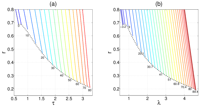
Figure 4: Gravitational shock absence in the single null fluid case. Panel (a) presents $r$ as a function of proper time $\tau$ along a family of ingoing radial timelike geodesics; panel (b) presents $r$ as a function of affine parameter $\lambda$ along a series of ingoing radial null geodesics. In both panels, geodesics are solid lines, distinguished by different colors and different timing parameter values; the timing parameter is $V_{h}$ (the value of initial ray RNV advanced time at the EH) for timelike geodesics and $V$ for null geodesics. Panel (a) contains timelike geodesics at the range $0\leq V_{h}\leq 80$, where $V_{h}$ increases by increments of $5$ from left $(V_{h}=0$) to right $(V_{h}=80)$; panel (b) contains grid null rays at the range $-3.3<V<95.7$, with irregular $V$ values and irregular increments of $V$ from left $(V\simeq-3.2)$ to right $(V\simeq 95.6)$. The dashed black curve denotes the corresponding IH value of the geodesics; $r_{-}(V_{h})$ in panel (a) and $r_{-}(V)$ in panel (b). Gravitational shock absence manifests in the smooth shape of $r(\tau)/r(\lambda)$.

5 TWO NULL FLUIDS CASE

We construct our two null fluids case through the inclusion of an outgoing null fluid pulse in the initial data setup described in Sec. 4.1. In addition to demonstrating the existence of a gravitational shock wave, we uncover some interesting results on the inner structure: a strong evidence for the existence of a spacelike $r=0$ singularity, and a possible indication for the existence of a null, non naked, $r=0$ singularity. The structure of this section is similar to the previous section with one exception: since our shock analysis has positive results, we provide an additional analysis of the shock sharpening rate, and compare it to MO and EO’s result.

5.1 Basic parameters and initial conditions

The initial spacetime in this case is the same as in the previous section — RN spacetime with mass parameter $M_{0}=1$ and charge parameter $Q=0.95$. The ingoing null fluid stream is also identical to the stream described in section 4.1; it has the same initial function $T_{vv}^{NF}$ on the initial outgoing ray $u=u_{0}$ (Eq. (15)) and the same parameters (begins at $r_{1}=10/v_{3}\approx 12.54/V_{3}\approx 5.63$ and has an amplitude of $A_{1}=3.4555203\times 10^{-4}$). However, we now include an outgoing null-fluid pulse, defined on the initial ingoing ray $v=v_{0}$ by

$$T_{uu}^{NF}(u,v_{0})=\begin{cases}\begin{array}[]{c}A_{2}\frac{16(r_{a}-r)^{3}(r-r_{b})^{3}}{\pi(r_{a}-r_{b})^{6}}r,_{u}^{2}\\ 0\end{array}&\begin{array}[]{c}|\,\,\,r_{b}\leq r\leq r_{a}\\ |\,\,\,\,otherwise.\end{array}\end{cases}$$ (16)

where $A_{2}$ is an amplitude parameter and $r,r,_{u}$ are functions of $u$ along the initial ray. The polynomial form has compact support and is limited to a certain $r$ range ($r_{b}\leq r\leq r_{a}$, which translates to a certain $u$ range, $u_{1}\leq u\leq u_{2}$) in order to control the mass function. The factor $r,_{u}^{2}$ allows us to avoid a numerical problem of “mass blow up” at the EH, a possible hazard of our gauge choice. We choose the amplitude as $A_{2}=12.0$, and the pulse limits as $r_{a}=1.54$ and $r_{b}=0.7$, which translates to $u_{1}\simeq 16.47$ and $u_{2}\simeq 253.72$. Since the EH is located at $u_{h}\simeq 69.29$ , the outgoing pulse begins well outside the BH and ends deep inside the BH; the location of the pulse and its general shape are illustrated in panel (a) of Fig. 5. Although the pulse has a simple shape in $r$, the factor $r,_{u}^{2}$ dampens it greatly at the vicinity of the EH; as a result, the effect of the pulse outside the BH turns out to be rather minor, while the effect inside the BH is much more pronounced, as demonstrated below. However, the outgoing pulse does decrease the mass of the BH, as now $m_{BH,vmax}=2.4925$. This mass fits EH value of $r_{+,vmax}\simeq 4.797$, IH value of $r_{-,vmax}\simeq 0.1881$, and surface gravity value of $\kappa_{-,vmax}$$\simeq 65.1$.

The remaining initial values are taken according to the second column of table 1. In particular, $T_{vv}^{NF}$ vanishes on $v=v_{0}$; $T_{uu}^{NF}$ vanishes on $u=u_{0}$; the scalar field $\Phi$ vanishes on both initial rays and $\sigma$ conforms on both rays with the maximal-$\sigma$ gauge condition (Eq. (9)).

The domain of integration is $u_{0}=v_{0}=0$, $u_{max}=253.7375$, and $v_{max}=120$. The value of $r$ in the initial vertex is $r_{0}=5$ and it grows up to $r\simeq 49.47$ at $r(u_{0},v_{max})$. The third corner of the grid is $r(u_{max},v_{0})\simeq 0.1326$; however, there are no numerical results available in the fourth corner of the grid $(u_{max},v_{max})$ due to the presence of a spacelike singularity.

5.2 The structure of spacetime

Fig. 5(b) reveals the complex structure of spacetime — it consists of eight patches of different effective spacetime (although only six are covered in our simulation). The initial RN patch (RN1) borders an outgoing null-fluid patch (RNVo) at $u=u_{1}$ and an ingoing null-fluid patch (RNVi) at $v=v_{3}.$ There are two additional RN patches: the asymptotic RN patch (RN2, at $u<u_{1}$ and $v>v_{4}$) is not covered in our simulation and has unknown mass parameter $m_{final}$; the inner RN patch (RN3, at $u>u_{2}$ and $v<v_{3}$) is located deep inside the BH (after the outgoing null-fluid pulse) and has mass parameter $m_{3}\approx 1.569$. The patch where the fluids intersect (TNF, at $u_{1}\leq u\leq u_{2}$, $v_{3}\leq v\leq v_{4})$ contains the shock wave and a spacelike $r=0$ singularity; we also see a possible indication for a section of null $r=0$ singularity, as we discuss below. There are additional single fluid patches where the null fluids separate, which are (in principle) extendable.

At first glance, the numerical results for $r(u,v)$ (Fig. 6) appears quite similar to the single null fluid case; panel (a), which displays results on the entire grid, seems almost identical to panel (a) of Fig. 3. A zoom near $u=u_{max}=253.7375$ (panels (b) and (c)) reveals a fundamental difference; while in the single null fluid case the grid ended regularly, in case of two null fluids we detect a $r=0$ singularity which breaks down the numerics (the border with the criss-cross patch, in which results are unavailable). The exact nature of this singularity is somewhat open to debate. While it clearly contains a spacelike section — the diagonal border of the criss-cross patch in panel (b), which extends from $v\sim 22$ up to $v_{max}=120$ — it may also contain a null ($v=const$) section, which is indicated at the top left of panel (b) and the focus of panel (c). If this is indeed a null section and not a different spacelike section, it is not well known; this is not a naked singularity which is a known phenomenon in Vaidya [34] and charged Vaidya [35, 36] geometries. The null classification is uncertain, however, mainly due to the proximity to the edge of the grid (where numerical fluxes may cause unexpected effects) and the short span of this section ($\sim 0.03$ in $u$). We also note that despite the way this section is drawn in Fig. 5, it is uncertain if this section begins at the end of the outgoing null fluid pulse $(u_{2}\simeq 253.72)$ or earlier. We conclude that this section (and the nature of singularities in this case in general) requires further study, which is beyond the scope of the current paper.

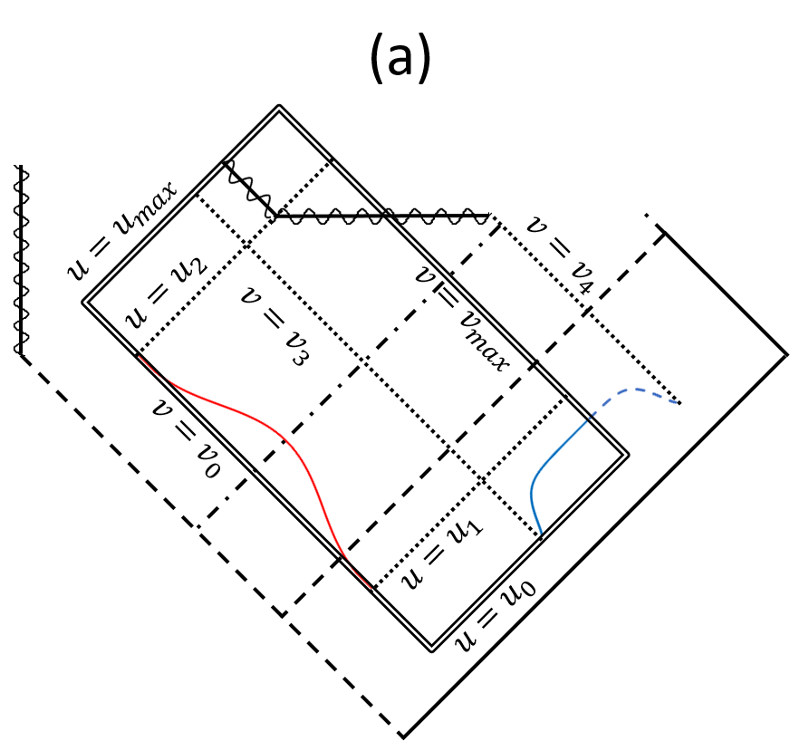
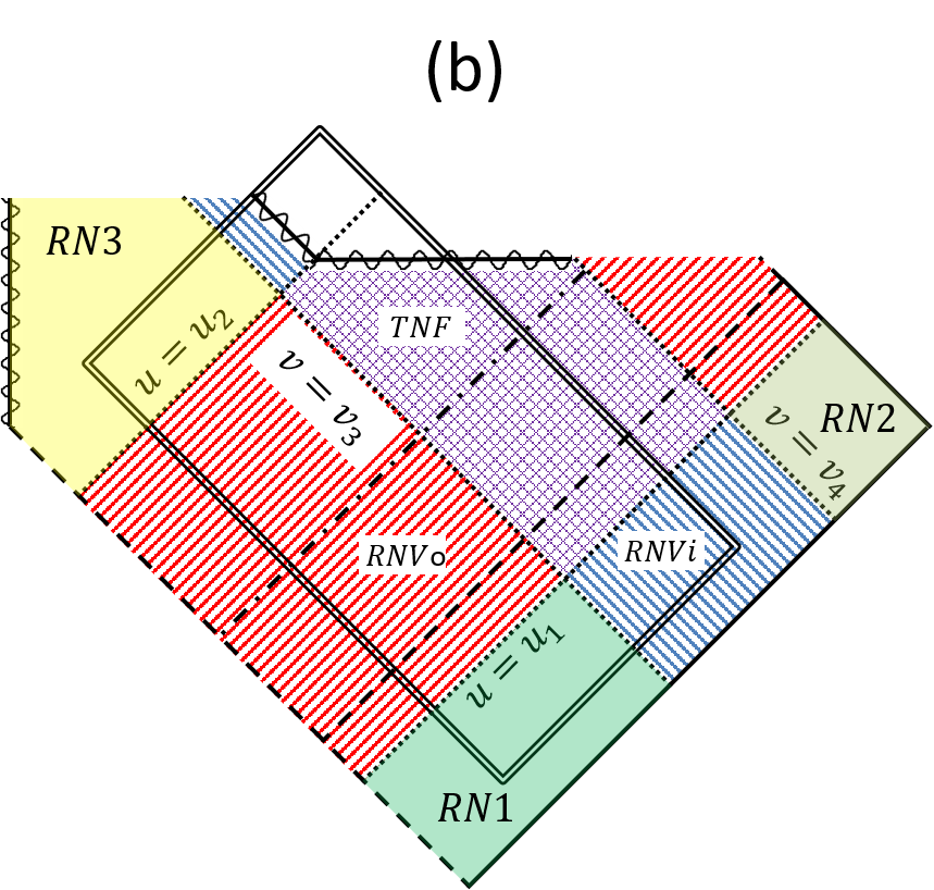
Figure 5: Penrose diagrams illustrating the structure of spacetime in the case of two null fluids. Both panels describe the location of the numerical domain of integration and the null fluids in spacetime; while panel (a) focuses on initial data, panel (b) analyzes the different patches of spacetime. In both panels, the domain’s limits are denoted by a double black line; solid black lines denote null infinity; dashed black lines denote the EH; dashed-dotted black lines denote the IH. Wavy lines denote the timelike $r=0$ singularity of RN geometry, as well as the spacelike $r=0$ singularity and the (suspected) null $r=0$ singularity that develop in this case. Dotted black lines denote the ingoing null-fluid stream limits $v=v_{3}$ and $v=v_{4}$, as well as the outgoing null-fluid pulse limits $u=u_{1}$ and $u=u_{2}$ . The blue curve in panel (a) represents the ingoing null-fluid stream on the initial ray $u=u_{0}$. The red curve represents the outgoing null-fluid pulse on the initial ray $v=v_{0}$; its shape roughly reflects the shape of the pulse in $T_{uu}$ but with a different choice for the coordinate $u$ (say, $u^{\prime}=-r(u,v_{0})$), which simplifies its form. Panel (b) demonstrates that spacetime could be divided into eight distinct patches: three patches of RN geometry (RN1, RN2 and RN3, initial, asymptotic and inner accordingly), two patches of ingoing null-fluid stream (RNVi, diagonal blue stripes), two patches of outgoing null-fluid pulse (RNVo, diagonal red stripes), and the patch in which both fluids intersect and the spacelike singularity develops (TNF, the checkered purple patch).

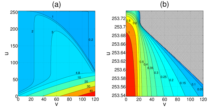
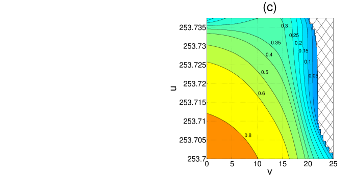
Figure 6: Numerical results for $r(u,v)$ in the case of two null fluids. The panels display contour graphs of $r(u,v)$ based on numerical results; panel (a) displays results on the entire grid; panel (b) displays a zoom deep inside the BH, near $u=u_{max}=253.7375$; panel (c) displays a further zoom on the top left corner of panel (b). Panel (a) uses different color code and different level choice for $r$ from panels (b) and (c) for the sake of visibility. The criss-cross patch on panels (b) and (c) represents a region in which numerical results are unavailable due to the $r=0$ singularity. Panel (b) reveals the presence of a spacelike $r=0$ singularity; it manifests as the diagonal border of the criss cross patch. Panels (b) and (c) hints on the presence of a null $r=0$ singularity, represented by the (approximately) vertical border of the criss-cross patch. Panel (a) is based on $N=640$ numerical results sampled in a lower resolution $(\Delta_{s}u=\Delta_{s}v=0.1)$, while panels (b) and (c) are based on $N=640$ numerical results without any sampling.

5.3 Gravitational shock detection

The gravitational shock wave is demonstrated in Figs. 7 and 8. Panel (a) of Fig. 7 presents $r(\tau)$ on a family of timelike geodesics; panel (b) displays $r(\lambda)$ on a series of null geodesics. In both cases the shock manifests as a sharp “break” or a vertical “drop” in $r(\tau)$/$r(\lambda)$, located at the specific crossing point of $r=r_{-}$ of the geodesic. Since the aforementioned “scale stretching” problem prevents a close inspection of the break (and obscures the shock), we draw the geodesics together by a simple shift in $r$ and $\tau/\lambda$ in panels (c) and (d) of Fig. 7. These panels display the same geodesics as panels (a) and (b) (accordingly), but each curve is now shifted by a different constant $r_{-}$ and a different constant $\tau/\lambda$; the shift by $r_{-}$ allows us to confirm more clearly that the shock is indeed located at the specific $r_{-}$ value of each geodesic.

The shock does not form immediately after the null fluid stream begins (at $V\simeq 5.63$). The first clear observation of the shock is seen in the timelike geodesic $V_{h}=20$ (Fifth from the left in panels (a)/(c)) or in the null geodesic $V=20.1$ (Fourth from the left in panels (b)/(d)). However, panels (c) and (d) indicate that once the shock forms it sharpens very quickly; for instance, it is hard to differentiate between the sharp features of timelike geodesics in the range $30\leq V_{h}\leq 70$ in panel (c).

While Fig. 7 demonstrates the shock very clearly (especially panels (c) and (d)), the visual effect remains somewhat limited: isolated and localized. We wish to reconstruct EO’s more global “vertical wall” representation of the shock. For this purpose, Fig. 8 presents $r(\lambda)$ of a series of null geodesics in a three-dimensional graph. The geodesics are taken from a similar $V$ range to the one in Fig. 7(b) but with a denser sampling. Panel (a) presents the exact $r(\lambda)$ curves of the geodesics; panel (b) presents the same geodesics, shifted by constant $r_{-}$ and $\lambda$ values in a similar fashion to panels (c) and (d) of Fig. 7. Although the earliest geodesics are smooth, we can see in panel (a) that each late geodesic “breaks” to a sheer drop at a different $r$ value. In panel (b) we confirm that this value is indeed the appropriate $r_{-}(V)$ value of the geodesic; we see the formation of the infamous “vertical wall”.

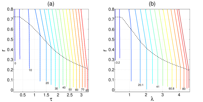
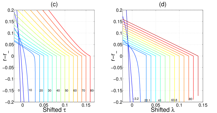
Figure 7: Gravitational shock wave in case of two null fluids. Panel (a) presents $r(\tau)$ for a family of radial timelike geodesics; panel (b) presents $r(\lambda)$ for a series of ingoing radial null geodesics. Geodesics are solid lines, distinguished by different colors and different timing parameter values; the timing parameter is $V_{h}$ for timelike geodesics and $V$ for null geodesics. The dashed black curve in panels (a) and (b) denotes the evolving IH value of the geodesics; $r_{-}(V_{h})$ in panel (a) and $r_{-}(V)$ in panel (b). Panel (c) displays the same timelike family of panel (a), but shifted in $r$ and $\tau$ [by subtracting the specific $r_{-}(V_{h})$ value of each geodesic from $r(\tau)$ and shifting $\tau$ by a constant factor ($\tau_{shift}=(i-1)\times 0.01-\tau_{f}^{(i)}$ for the $i$-th geodesic from the left, where $i=1,...17$ and $\tau_{f}^{(i)}$ is the last proper time value of the geodesic)]. Panel (d) displays the same null series of panel (b), but shifted in $r$ and $\lambda$ in a similar fashion [subtraction of the specific $r_{-}(V)$ value of each geodesic from $r(\lambda)$ and a shift of $\lambda$ by $\lambda_{shift}=(i-1)\times 0.01-\lambda_{f}^{(i)}$ for the $i$-th geodesic from the left, where $i=1,...15$ and $\lambda_{f}^{(i)}$ is the last affine parameter value of the geodesic). Panels (a) and (c) contain timelike geodesics at the range $0\leq V_{h}\leq 80$, where $V_{h}$ increases by increments of $5$ from left $(V_{h}=0$) to right $(V_{h}=80)$; panels (b) and (d) contain grid null rays at the range $-3.3<V<92.6$, with irregular $V$ values and irregular increments of $V$ from left $(V\simeq-3.2)$ to right $(V\simeq 92.5)$. Gravitational shock manifests as a sharp drop or “break” in $r(\tau)/r(\lambda)$ at the IH; the shock is first seen clearly on $V_{h}=20/V=20.1$, and is easier to observe in panels (c) and (d).

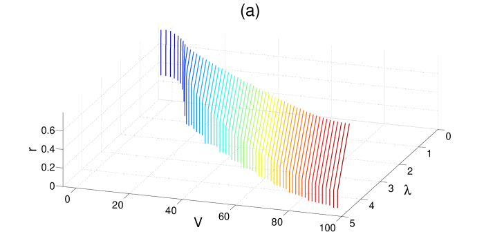
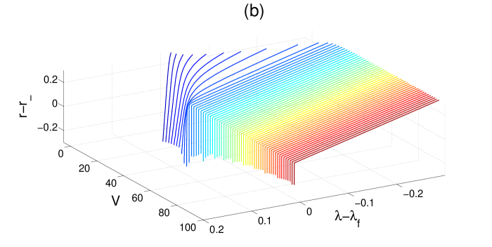
Figure 8: Gravitational shock wave in case of two null fluids. Panel (a) displays $r(\lambda)$ for a series of ingoing radial null geodesics; panel (b) displays the same set of geodesics, shifted in $r$ and $\lambda$ in a similar fashion to Fig. 7(d); here we subtract the specific $r_{-}(V)$ value of each geodesic from its $r(\lambda)$ and shift $\lambda$ by $-\lambda_{f}$ (the specific final $\lambda$ value of the geodesic). The geodesics are solid lines, distinguished by different colors. The set consists of grid null rays at the range $-3.3<V<95.7$ with irregular $V$ values and increments of $V$; the series of Fig. 7(b) is a subset of this series. In both panels the results are cut in $r$ and $\lambda$ in order to allow visibility. The shock manifests as a sharp “break” or drop in $r(\lambda)$ at the IH ($r_{-}(V)$). Panel (b) demonstrates this better due to the shift.

5.4 Shock sharpening rate

MO predicted from analytical considerations that any characteristic $\Delta\tau$ width of the shock is expected to decrease exponentially according to $\Delta\tau\sim e^{-\kappa_{-}v_{eh}}$, where $\kappa_{-}$ was the constant RN (or Kerr) surface gravity at the IH and $v_{eh}$ was their timing parameter for timelike geodesic — the value of Eddington advanced time coordinate at the EH. EO have confirmed MO prediction numerically. We do not expect this relation to hold in our case since we have a slowly growing surface gravity at the IH. We also have different timing parameters, the aforementioned $V_{h}$ and $\widetilde{V}_{f}$ (defined at Sec. 3.1.3 and as yet unused). We expect that if we chose our timing parameters wisely they should admit a simple analytical expression for the shock sharpening rate.

In order to analyze the sharpening rate, we first need to define a specific characteristic $\Delta\tau$ width of the shock. We again follow EO ansatz and define $\Delta\tau$ as the proper time duration to drop from $0.75r_{-}(v)$ to $0.25r_{-}(v)$ along the geodesic. Fig. 9 presents the rapid decrease in this characteristic width as a function of the timing parameter $V_{h}$. Each point in this figure represents the characteristic shock width of a single timelike geodesic from Fig. 7(a); our characteristic width is unavailable for geodesics in the range $V_{h}<25$ since they do not reach $r=0.25r_{-}(v)$ in our simulation. The decrease in $\ln(\Delta\tau)$ is very rapid, reaching extreme orders of $\ln(\Delta\tau)\sim-1200$; the non-linear pattern of the decrease confirms our suspicion that the simple exponential law of MO is no longer valid.

We consider two new generalized sharpening rate laws in Fig. 10, each associated with a different timing parameter. We consider the possible sharpening rate law $\Delta\tau\sim e^{-\intop\kappa_{-}(V_{h})\,dV_{h}}$ in panel (a), by comparing $\kappa_{-}(V_{h})$ to the derivative $-\frac{d\ln(\Delta\tau)}{dV_{h}}$; we consider the possible law $\Delta\tau\sim e^{-\intop\kappa_{-}(\widetilde{V}_{f})\,d\widetilde{V}_{f}}$ in panel (b) by comparing $\kappa_{-}(\widetilde{V}_{f})$ to the derivative $-\frac{d\ln(\Delta\tau)}{d\widetilde{V}_{f}}$. The derivatives and $\kappa_{-}$ curves were calculated using Matlab spline cubic interpolation. Both sharpening rate laws offers a match that seems too good to be coincidental; we argue that the second sharpening rate law offers a slightly better match due to a better asymptotic match.

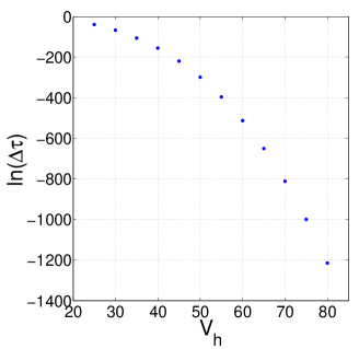
Figure 9: Gravitational shock width decrease in the case of two null fluids. The graphs presents $\ln(\Delta\tau)$ as a function of the timing parameter $V_{h}$. Each point represents a single radial timelike geodesic from the family of Fig. 7(a) (at the range $25\leq V_{h}\leq 80$, where $V_{h}$ increases by increments of $5$). The nonlinear behaviour of $\ln(\Delta\tau)$ suggests that the original MO’s linear relation indeed breaks as expected due to the change in $\kappa_{-}(V_{h}).$

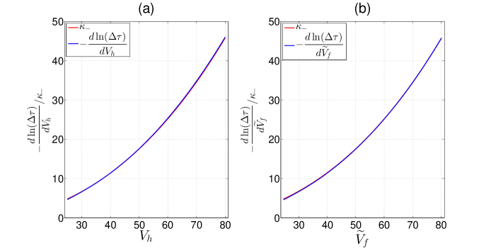
Figure 10: Shock sharpening rate in the case of two null fluids. Panel (a) tests the possible connection $\Delta\tau\sim e^{-\intop\kappa_{-}(V_{h})\,dV_{h}}$ by comparing the increasing $\kappa_{-}(V_{h})$ to the derivative $-\frac{d\ln(\Delta\tau)}{dV_{h}}$; panel (b) tests the possible connection $\Delta\tau\sim e^{-\intop\kappa_{-}(\widetilde{V}_{f})\,d\widetilde{V}_{f}}$ by comparing $\kappa_{-}(\widetilde{V}_{f})$ to the derivative $-\frac{d\ln(\Delta\tau)}{d\widetilde{V}_{f}}$. Both relations provide a fairly good match; we argue there is a slight advantage for the second ($\Delta\tau\sim e^{-\intop\kappa_{-}(\widetilde{V}_{f})\,d\widetilde{V}_{f}}$ of panel (b)), due to a better asymptotic match. The calculations of the derivatives and $\kappa_{-}$ curves are based on Matlab cubic spline interpolation of data from the geodesics of Fig. 9.

6 THE MIXED CASE: AN INGOING NULL FLUID WITH A SELF GRAVITATING SCALAR FIELD

We construct our mixed case through the addition of an ingoing self-gravitating scalar-field pulse to the initial data setup described in Sec. 4.1. We also slightly modify our ingoing null-fluid stream in order to preserve its mass contribution. EO have already demonstrated the existence of a gravitational shock in the self-gravitating scalar-field case; here we are interested in the effect of the null-fluid stream on a previously generated shock. Again, we demonstrate the shock presence and analyze its sharpening rate by the same methods of the previous section.

6.1 Basic parameters and initial conditions

The initial RN spacetime has the same parameters as in the previous two cases — initial mass parameter of $M_{0}=1$ and charge parameter of $Q=0.95$. We define an ingoing self-gravitating scalar-field pulse on the initial ray $u=u_{0}$ in the same fashion as EO did,

$$\Phi(u_{0},v)=\begin{cases}\begin{array}[]{c}A_{3}\frac{64(v-v_{1})^{3}(v_{2}-v)^{3}}{(v_{2}-v_{1})^{6}}\\ 0\end{array}&\begin{array}[]{c}|\,\,\,v_{1}\leq v\leq v_{2}\\ |\,\,\,otherwise\,,\end{array}\end{cases}$$ (17)

where $A_{3}$ is an amplitude parameter. Similar to the outgoing null-fluid pulse from the previous section, this scalar-field pulse has compact support on the initial ray $u=u_{0}$, and is limited to a certain $v$ range, $v_{1}\leq v\leq v_{2}$. We choose $v_{1}=1$ and $v_{2}=7$ (like EO did) but a slightly higher value of $A_{3}$ than EO’s ($A_{3}=0.1201$) in order to set the mass contribution of the pulse to the BH to be $\Delta m_{\Phi,vmax}\simeq 0.5$. The relative location of the pulse and its shape are illustrated in panel (a) of Fig. 11. The ingoing null fluid stream has the same form of Eq. (15), but we slightly raise its amplitude as well (to $A_{1}=4.267591\times 10^{-4}$) in order to preserve the mass contribution to the BH ($\Delta m_{NF,vmax}\simeq 1.5$). The stream begins at $r_{1}=10$, which is now equivalent to $v_{3}\simeq 14.77$ or $V_{3}\simeq 7.35$. Overall we get a BH with a mass of $m_{BH,vmax}\simeq 3.0$; the corresponding EH and IH values are $r_{+,vmax}\simeq 5.846$ and $r_{-,vmax}\simeq 0.1544$, and the corresponding IH surface gravity is $\kappa_{-,vmax}\simeq 119.4$. The EH is reached earlier than the previous two cases, at $u_{h}\simeq 42.9$.

The remaining initial values are taken according to the third column of table 1. In particular, $T_{vv}^{NF}$ vanishes on $v=v_{0}$; $T_{uu}^{NF}$ vanishes on both initial rays; the scalar field $\Phi$ vanishes on $v=v_{0}$ and $\sigma$ conforms on both rays with the maximal-$\sigma$ gauge condition (Eq. (9)).

The domain of integration is $u_{0}=v_{0}=0$, $u_{max}=298.65$, and $v_{max}=120$. The value of $r$ in the initial vertex is $r_{0}=5$ and it grows up to $r\simeq 40.02$ at $r(u_{0},v_{max})$. The third corner of the grid is $r(u_{max},v_{0})\simeq 0.1003$; the fourth corner $(u_{max},v_{max})$ is located (again) beyond a spacelike singularity.

6.2 The structure of spacetime

The structure of spacetime in this case (displayed on Fig. 11) is simpler than the case of two null fluids in several respects: there are only four patches of spacetime, and only three of them are covered in our simulation; the borders between the patches are always $v=const$ rays; spacetime is (mostly) non extendable due to presence of a (well known) spacelike $r=0$ singularity. The initial RN patch ends at $v=v_{1}$; it is followed by perturbed charged patch (PC1) which contains a self gravitating scalar-field perturbation. The spacelike singularity and the gravitational shock wave originate from this patch; it ends at the beginning of the null fluid stream at $v=v_{3}$. The second perturbed charged patch (PC2) contains the null fluid stream as well as the (slowly decaying) scalar-field; this is the most interesting patch to us, and it ends with the null fluid stream at $v=v_{4}$. The last perturbed charged patch (PC3) contains, again, just the slowly decaying scalar field. Asymptotically, the geometry of this patch outside the BH and at the close vicinity of the EH is RN geometry with some unknown mass $m_{final}$. This patch is not covered in our simulation.

The numerical results for $r(u,v)$ (Fig. 12) demonstrate the spacelike $r=0$ singularity very clearly; this time it is even noticeable at the full grid level (panel (a)), although a closer zoom (panel (b)) is needed in order to reveal its spacelike nature (the curved shape of the border of the criss cross patch). This zoom also offers us some puzzlement in the form of two seemingly null sections of the singularity; one vertical $v=const$ section of the border (begins at $u\sim 295$) and one horizontal $u=const$ section of the border (begins at $v\sim 7$). We focus on these sections on panels (c) and (d). We argue that these sections are not likely to represent true null singularity sections, however, for several reasons. Panels (c) and (d) reveal a smooth transition between these sections and spacelike sections; the truly null sections appear much shorter in these panels. The quick succession of null-spacelike-null-spacelike sections raises further skepticism. Lastly, these sections are located mostly in the patch PC1, before the null fluid stream (the vertical section is entirely in PC1; the horizontal section ends at $v\sim 15$, where PC2 begins at $v\simeq 14.77$); scalar-field perturbation is not known to generate null $r=0$ singularities. We tend to conclude that these sections are actually spacelike sections and suggest that the changes in appearance of the spacelike singularity represent changes of phases in spacetime [e.g. the end of the main scalar field pulse (on $v=7$ at $u=u_{0}$, slightly later on higher $u$ values), and the beginning of the null fluid stream]. We are aware this explanation raises further doubts regarding the nature of the suspected null $r=0$ singularity in the two null fluids case (Sec. 5.2); we have already agreed that further research is needed in order to confirm its existence.

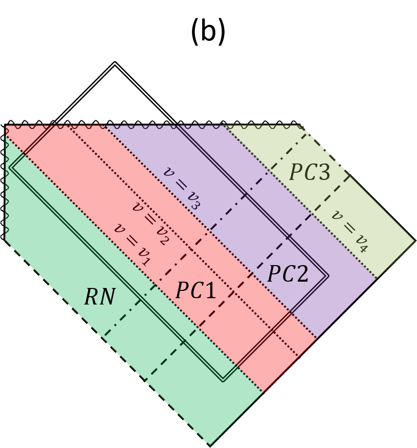
Figure 11: Penrose diagrams illustrating the structure of spacetime in the mixed case. Both panels describe the location of the numerical domain of integration and the different perturbations in spacetime; while panel (a) focuses on initial data, panel (b) analyzes the different patches of spacetime. In both panels, the domain’s limits are denoted by a double black line; solid black lines denote null infinity; dashed black lines denote the EH; dashed-dotted black lines denote the IH. Wavy lines denote the timelike $r=0$ singularity of the initial RN geometry, as well as the spacelike $r=0$ singularity that develops in this case. Dotted black lines denote the limits of the ingoing scalar-field pulse on the initial ray $u=u_{0}$ ($v=v_{1}$ and $v=v_{2}$) and the ingoing null-fluid stream limits $v=v_{3}$ and $v=v_{4}$. The blue curve in panel (a) represents the ingoing null-fluid stream on the initial ray $u=u_{0}$. The red curve represents the ingoing scalar-field pulse on the same initial ray; its shape reflects directly the shape of the pulse in $\Phi$. Panel (b) demonstrates that spacetime could be divided into four distinct patches: one patch of initial RN geometry (RN), and three patches of perturbed charged geometry (PC1, PC2 and PC3). PC1 and PC3 are perturbed only by the scalar field; PC2 is perturbed by the null fluid stream and the scalar field. The patch PC3 is not covered in our simulation and has asymptotically RN geometry outside the BH (and at the close vicinity of the EH).

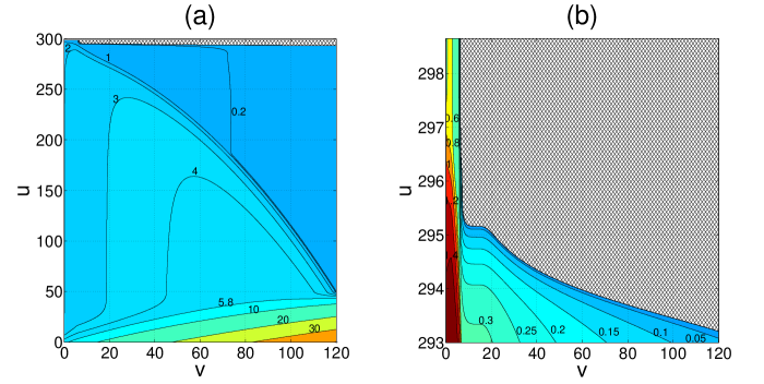
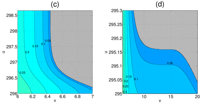
Figure 12: Numerical results for $r(u,v)$ in the mixed case. The panels display contour graphs of $r(u,v)$ based on numerical results; panel (a) displays results on the entire grid; panel (b) displays a zoom deep inside the BH, near $u=u_{max}=298.65$; panels (c) and (d) display further zooms on panel (b). Panel (a) uses different color code and different level choice for $r$ from panels (b)-(d) for the sake of visibility. The criss-cross patch in all panels represents a region in which numerical results are unavailable due to the $r=0$ singularity. Panel (b) reveals the presence of a spacelike $r=0$ singularity; it manifests as the curved border of the criss cross patch. There are also a horizontal section and a vertical section of the border in panel (b) that could have hinted on the existence of two sections of null singularity; we argue in the text that this is not likely here. Panels (c) and (d) focus on these sections. Panel (a) is based on $N=640$ numerical results sampled in a lower resolution $(\Delta_{s}u=\Delta_{s}v=0.1)$; panel (b) is based on $N=640$ results with a sampling on $v$ alone $(\Delta_{s}v=0.05)$; panels (c) and (d) are based on $N=640$ results without any sampling.

6.3 Gravitational shock detection

The gravitational shock wave is demonstrated in Figs. 13 and 14. Panels (a) and (c) of Fig. 13 display the shock in $r(\tau)$ of timelike geodesics; panels (b) and (d) display the shock in $r(\lambda)$ of null geodesics. Again, panels (c) and (d) display the same geodesics as panels (a) and (b) but with a shift in $r$ and $\tau/\lambda$ in order to allow clearer observation of the shock. The general picture is very similar to the case of two null fluids; the shock manifests as a clear vertical drop in $r(\tau)/r(\lambda)$, located at the appropriate $r_{-}$ value of the geodesic. The main difference is that now the shock begins earlier, due to the scalar-field pulse; it could be observed as early as the timelike geodesic $V_{h}=5$ or the null geodesic $V=8.4$. In panels (a) and (b), one could notice the short break between the end of the scalar field pulse and the beginning of the null fluid stream on which $r_{-}$ is roughly constant; this break is located between the timelike geodesics $V_{h}=0$ and $V_{h}=5$ in panel (a) and the null geodesics $V=1$ and $V=8.4$ in panel (b). After this break $r_{-}(v)$ continues to decrease.

We demonstrate the “vertical wall” representation of the shock through null geodesics in a three-dimensional graph in Fig. 14. Panel (a) displays the true $r(\lambda)$ curves of the geodesics while panel (b) displays shifted curves. Again, we use geodesics from the same range of Fig. 13(b) but with a denser sampling. Here, unlike the case of two null fluids, all the geodesics seem “broken”, each one breaks to a sheer drop at a different $r$ value. Panel (b) confirms that this is indeed the right $r_{-}(V)$ value.

Figure 13: Gravitational shock wave in the mixed case. Panel (a) presents $r(\tau)$ for a family of radial timelike geodesics; panel (b) presents $r(\lambda)$ for a series of ingoing radial null geodesics. Geodesics are solid lines, distinguished by different colors and different timing parameter values; the timing parameter is $V_{h}$ for timelike geodesics and $V$ for null geodesics. The dashed black curve in panels (a) and (b) denotes the evolving IH value of the geodesics; $r_{-}(V_{h})$ in panel (a) and $r_{-}(V)$ in panel (b). Panels (c) and (d) display the same set of geodesics as panels (a) and (b) (accordingly) but shifted by constant factors in the same fashion as panels (c) and (d) of Fig. 7. Panels (a) and (c) contain timelike geodesics at the range $0\leq V_{h}\leq 75$, where $V_{h}$ increases by increments of $5$ from left $(V_{h}=0$) to right $(V_{h}=75)$; panels (b) and (d) contain grid null rays at the range $0<V<81.5$, with irregular $V$ values and irregular increments of $V$ from left $(V\simeq 1)$ to right $(V\simeq 81.4)$. Gravitational shock manifests as a sharp drop or “break” in $r(\tau)/r(\lambda)$ at the IH; the shock is first seen clearly on $V_{h}=5/V=8.4$ (the second geodesic from the left in panels (a) and (c)/panels (b) and (d)), and is easier to observe in panels (c) and (d).

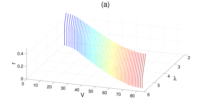
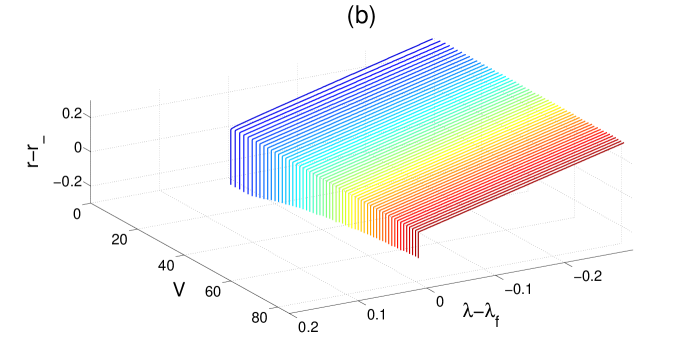
Figure 14: Gravitational shock wave in the mixed case. Panel (a) displays $r(\lambda)$ for a series of ingoing radial null geodesics; panel (b) displays the same set of geodesics, shifted in $r$ and $\lambda$ in a similar fashion to Fig. 8(b). The geodesics are solid lines, distinguished by different colors. The set consists of grid null rays at the range $0<V<81.5$ with irregular $V$ values and increments of $V$; the series of Fig. 13(b) is a subset of this series. In both panels the results are cut in $r$ and $\lambda$ in order to allow visibility. The shock manifests as a sharp “break” or drop in $r(\lambda)$ at the IH ($r_{-}(V)$). Panel (b) demonstrates this better due to the shift.

6.4 Shock sharpening rate

We turn next to analyze the sharpening rate of the shock by the same method used in Sec. 5.4. Fig. 15 presents the decrease in the characteristic width of the shock $\Delta\tau$ (the same width defined in Sec. 5.4). Each point represents a single timelike geodesic from Fig. 13(a); in this case we have characteristic widths for all of them. The decrease in $\ln(\Delta\tau)$ is extreme, reaching orders of $\ln(\Delta\tau)\sim-3250$. Fig. 16 considers the same two suggested sharpening rate laws as Fig. 10, $\Delta\tau\sim e^{-\intop\kappa_{-}(V_{h})\,dV_{h}}$ in panel (a) and $\Delta\tau\sim e^{-\intop\kappa_{-}(\widetilde{V}_{f})\,d\widetilde{V}_{f}}$ in panel (b), by checking the relevant matches between $\kappa_{-}$ and the derivative of $-\ln(\Delta\tau)$. The match for both laws is, again, fairly good but not perfect; we notice a clear difference between the curves of $\kappa_{-}$ and the derivatives in the early phase ($V_{h}\apprle 30,\widetilde{V}_{f}\lesssim 45$) as well as additional difference for the first law at interim $V_{h}$ values $(40\apprle V_{h}\apprle 70)$. We (again) argue that the second connection ($\Delta\tau\sim e^{-\intop\kappa_{-}(\widetilde{V}_{f})\,d\widetilde{V}_{f}}$) provides a better description of the sharpening rate due to the better match between $\kappa_{-}$ and the relevant derivative of $-\ln(\Delta\tau)$.

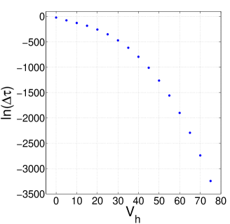
Figure 15: Gravitational shock width decrease in the mixed case. The graphs presents $\ln(\Delta\tau)$ as a function of the timing parameter $V_{h}$. Each point represents a single radial timelike geodesic from the family of Fig. 13(a) (at the range $0\leq V_{h}\leq 75$, where $V_{h}$ increases by increments of $5$).

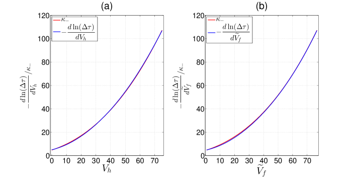
Figure 16: Shock sharpening rate in the mixed case. We test the same connections as in Fig. 10; panel (a) tests $\Delta\tau\sim e^{-\intop\kappa_{-}(V_{h})\,dV_{h}}$ and panel (b) tests $\Delta\tau\sim e^{-\intop\kappa_{-}(\widetilde{V}_{f})\,d\widetilde{V}_{f}}$. Again, both relations provide a fairly good match but the second ($\Delta\tau\sim e^{-\intop\kappa_{-}(\widetilde{V}_{f})\,d\widetilde{V}_{f}}$ of panel (b)), offers a better asymptotic match. The calculations of the derivatives and $\kappa_{-}$ curves are based on Matlab cubic spline interpolation of data from the geodesics of Fig. 15.

7 DISCUSSION

Although we did not observe the gravitational shock wave in the single null fluid case, we have detected it in the case of two null fluids and in the mixed ingoing null-fluid/self-gravitating scalar-field case. In both cases the shock manifests as a sharp break or a sheer drop in $r(\tau)$ (or $r(\lambda)$) of timelike (or null) geodesics, located at the crossing point of $r=r_{-}(v)$ of the geodesic. $r_{-}(v)$ decreases monotonically due to null fluid accretion; the match between the shock location to $r=r_{-}(v)$ is conserved throughout the process. The characteristic width of the shock $\Delta\tau$ decreases rapidly in both cases. Since MO’s original sharpening rate law is no longer valid, we have tested two generalized sharpening rate laws through a match between $\kappa_{-}$ curve and the relevant derivatives of $-\ln(\Delta\tau)$. We have discovered that the generalized sharpening rate law $\Delta\tau\sim e^{-\intop\kappa_{-}(\widetilde{V}_{f})\,d\widetilde{V}_{f}}$ offers a fairly good match to the shock sharpening rate in both cases, though not perfect. In addition, we have gained new insight into the inner (classical) structure of the BH in the case of two null fluids perturbation; our numerical $r(u,v)$ results provided strong evidence for the existence of a spacelike $r=0$ singularity, and a possible indication for the existence of a null non-naked $r=0$ singularity, although this indication is uncertain and requires further research.

Our gravitational shock differs from the one EO discussed (in the self-gravitating scalar field case) in two main respects. Our $r_{-}(v)$ decreases due to long term accretion; EO observed MO original sharpening rate law of the shock, $\Delta\tau\sim e^{-\kappa_{-}v_{eh}}$ , while we observed a generalized law ($\Delta\tau\sim e^{-\intop\kappa_{-}(\widetilde{V}_{f})\,d\widetilde{V}_{f}}$), although it follows immediately that EO sharpening rate law is just a private case of our generalized sharpening rate in the case of a constant $\kappa_{-}$, with the proper change in timing parameter selection.

The existence of a spacelike $r=0$ singularity in case of two null fluids perturbation is not entirely surprising. Besides the well known spacelike singularity of the self-gravitating scalar-field case, [10, 15] a spacelike singularity is known to develop in a special two null fluids case, where the ingoing and the outgoing null fluid fluxes are equal and time-independent; [37, 38, 39] in this case spacetime is homogenous and a spacelike singularity develops from the outset, without a null singularity at the CH at all. In our two null fluids case, however, the fluxes are unequal (and time dependent); as far as we are aware of, the existence of a spacelike $r=0$ singularity in this case has not been demonstrated before in publications.

The minor mismatch in our sharpening rate law graphs (the differences between the curve of $\kappa_{-}$ and the curves of the derivatives of $-\ln(\Delta\tau)$) may be caused by timing parameter choice. We discuss at some length in Sec. A.1 of the appendix the differences between the variants of RNV advanced time; we argue that $\widetilde{V}$ should be a “better” RNV coordinate than $V$ deep inside the BH (at the shock region) as it is calculated closer to the shock. (similar argument should also apply on the choice to evaluate the timing parameter at the shock location instead of the EH crossing). It follows logically that $\widetilde{V}_{f}$ is a better timing parameter than $V_{h}$ as it describes the dynamics of spacetime inside the BH more accurately. But what if the “right” timing parameter actually belongs to a third variant of RNV advanced time coordinate, calculated in the vicinity of the shock instead of the EH? Such calculation is technically problematic in the current version of the code, but may resolve some of the differences between the curves. In the mixed case we have an even better reason to doubt the accuracy of our timing parameters choice; as discussed in the appendix, at the early stages of the simulation, when the scalar field is dominant, the coordinates of our timing parameters are not “good” RNV coordinates, only approximated RNV coordinates; thus we expect them to be less successful in describing accurately the development of the shock at this stage. Indeed, the mismatch in the mixed case is very dominant in the early stage. The mismatch may be, in theory, an artifact of our cubic spline interpolation procedure; we do not believe this to be the case since the interpolated series of Figs. 9 and 15 seem to describe a reasonably smooth function sampled at a decent resolution. Moreover, the mismatch is more obvious at low values of the timing parameter $V_{h}$ and the function $\ln(\Delta\tau)$ is actually milder there.

We recognize two possible issues that could potentially compromise the reliability of our numerical results. The first issue is the fact that our simulation is entirely classical, while we expect Quantum Gravity to become relevant at the close vicinity of the $r=0$ singularity. The second issue is the decline in performance of the numerical solver near this singularity (discussed in Sec. 3). We argue that while Quantum Gravity may replace the $r=0$ singularity with a regular extension of spacetime, it is irrelevant for our shock results, and even for the general location of the (would be) $r=0$ spacelike singularity. We demonstrate this by a simple calculation of Planck length in our units ($c=G=M_{0}=1$). From units considerations, the reduced Planck constant satisfy $\hbar\propto GM_{0}^{2}/c$, so we can find that in our units $\hbar\approx 4.74\times 10^{-78}$. Planck length turns out to be a square root of this number in our units since $l_{P}=\sqrt{\frac{\hbar G}{c^{3}}}\approx 2.18\times 10^{-39}$. This number is many orders of magnitude below the lowest $r$ value in which we maintain numerical reliability (of order $r\sim 10^{-2}$).

We classify our numerical results into three categories of numerical reliability. We consider the shock detection results to be highly reliable: (i) they are confirmed by two different and independent mechanisms, results on timelike and null geodesics; (ii) they begin quite far from the $r=0$ singularity ($r\approx 0.48$ in the case of two null fluids perturbation, $r\approx 0.34$ in the mixed case); (iii) they are supported by numerical convergence indicators (e.g. the overlap of $N=320$ and $N=640$ timelike geodesics results in Figs. 4(a), 7(a) and 13(a)). The second category contains results we consider reliable: the detection of a spacelike $r=0$ singularity in the case of two null fluids and our sharpening rate law analysis. The exact location of the spacelike singularity might be slightly distorted due to numerical performance (or resolution limits) issues, but its spacelike nature is a clear and consistent feature across the grid. Our sharpening rate analysis is based on highly reliable timelike geodesics data but involves an interpolation mechanism which may slightly distort the curves shape, but not alter the basic match between the curves of $\kappa_{-}$ and the derivatives of $-\ln(\Delta\tau)$ (also, since both $\kappa_{-}$ and the derivative curves are interpolated in the same fashion, they are unlikely to be distorted in different directions). As we have already elaborated, the detection of a null $r=0$ section of the singularity in the case of two null fluids belongs to the third category — it is uncertain and requires further research.

Our research could be extended in many directions. Due to the limited scope of this paper, we have focused our attention on the gravitational shock (or the shock in the metric function $r$). Nevertheless, the shock is expected to manifest in the scalar field as well. It could be interesting to analyze the effect of the null fluid stream on the shock in the scalar field $\Phi$ in the mixed case, as a “toy model” for interaction between two different types of perturbations in the context of the shock; astrophysical BHs are expected to accrete matter as well as radiation. It could also be enlightening to study how the shock manifests, if at all, in various curvature scalars; MO and EO have not discussed their behaviour specifically in the context of the shock, but equivalent studies have been made regarding CH, a well known curvature singularity in the perturbed charged (or spinning) case (see e.g. Ref. [26] for a recent numerical study in Kerr).

We believe that the most acute next step in the numerical study of the shock is the extension of the research to spinning BHs. Astrophysical BHs are expected to be spinning; for instance, in recently detected gravitational waves events GW150914 [40] and GW151226, [41] the outcome of the mergers was BHs with a significant spin, $a/m\sim 0.7$. As far as we are aware, there had been no numerical verification of the shock existence in the spinning case. This numerical study would be extremely challenging due to the lack of spherical symmetry.

A different research direction stemming from our research is the numerical study of the inner structure of charged BHs perturbed by two null fluids. Possible concrete objectives are determining the exact nature of the spacelike $r=0$ singularity and the possible existence of a null, non-naked $r=0$ singularities. This research would require an improvement in the numerical performance of our algorithm near the singularity; both the ODE solver of the constraint equation on the initial ray $u=u_{0}$ (Eq. (6)) and the grid bulk solver of the PDEs need to be “immunized” against the singularity. A possible mechanism may be a special gauge selection. EO have used a special gauge variant of the maximal-$\sigma$ gauge, called the singularity approach gauge. This variant was intended to resolve the approach to a contracting CH on the grid final ray $v=v_{max}$. If this gauge could be generalized to resolve any approach to $r=0$ (on any $v$ value), it should be a suitable candidate for this research.

Appendix A Appendix: RNV advanced time coordinate

A.1 Definition, numerical calculation and interpretation

The definition and calculation of RNV advanced time coordinate is identical for all the scenarios in this paper, although the meaning and the interpretation of the coordinate differ. We now describe spacetime with a new metric, the ingoing RNV metric. The line element is defined (in the coordinates $(V,r,\theta\varphi))$ as

$$ds^{2}=-(1-\frac{2m(V)}{r}+\frac{Q^{2}}{r^{2}})dV^{2}+2dVdr+r^{2}d\Omega^{2}\,.$$ (18)

In order to find RNV advanced time coordinate $V$ as a (numerical) function of the numerical coordinate $v$, we have applied two different methods: (i) we calculated $V$ using the coordinate transformation from RNV metric to our metric (given by the line element of Eq. (1)); (ii) we considered an outgoing null ray that satisfies $ds^{2}=0$ and $d\Omega^{2}=0$. The results of these two independent calculations are denoted below as $V_{a}(v)$ and $V_{b}(v)$, accordingly. We hereby explain both methods and demonstrate that they yield consistent results.

The standard metric coordinate transformation satisfies $g^{\prime}_{\mu\nu}=g_{\alpha\beta}\frac{\partial x^{\alpha}}{\partial x^{\mu}}\frac{\partial x^{\beta}}{\partial x^{\nu}}$. In particular, since $\frac{\partial V}{\partial u}=0$, $g_{uv}$ yields

$$g_{uv}=-\frac{e^{\sigma}}{2}=g_{\alpha\beta}\frac{\partial x^{\alpha}}{\partial u}\frac{\partial x^{\beta}}{\partial v}=\frac{\partial r}{\partial u}\frac{\partial V}{\partial v}\,.$$

We can isolate $\frac{\partial V}{\partial v}$ and integrate to obtain

$$V_{a}(v)=-\intop\frac{e^{\sigma}}{2r,_{u}}\,dv\,.$$ (19)

Alternately, we may consider an outgoing null ray $u=const$. Since this geodesic satisfies $ds^{2}=0$ and $d\Omega^{2}=0$, we obtain from the line element (Eq. (18))

$$2dVdr=(1-\frac{2m(V)}{r}+\frac{Q^{2}}{r^{2}})dV^{2}\,.$$

Now we can isolate $\frac{dV}{dr}$ and integrate to obtain

$$V_{b}(v)=\intop\frac{2}{(1-\frac{2m(V)}{r}+\frac{Q^{2}}{r^{2}})}\,dr\,.$$ (20)

In both methods the integration is performed retroactively, after the functions $r,_{u}(v),\>r(v)$ and $m(v)$ are known. We use a simple numerical integration scheme that replaces Eq. (19) with

$$V_{a}(v+\Delta v)=V_{a}(v)-\frac{e^{(\sigma(v)+\sigma(v+\Delta v))/2}}{r,_{u}(v)+r,_{u}(v+\Delta v)}\Delta v\,,$$ (21)

and Eq. (20) with

$$V_{b}(v+\Delta v)=V_{b}(v)+\frac{4\Delta r}{2-\frac{2m(v)}{r(v)}-\frac{2m(v+\Delta v)}{r(v+\Delta v)}+\frac{Q^{2}}{r(v)^{2}}+\frac{Q^{2}}{r(v+\Delta v)^{2}}}\,.$$ (22)

This integration scheme is second order accurate. We fix the integration constant, or the origin of the coordinate, by the choice to identify $V=0$ with the end of the scalar-field pulse in the mixed case $(v=7)$. We opted to keep this choice in the single null fluid case and the two null fluids case as well, despite the absence of the scalar-field pulse, for the sake of uniformity.

In principle, the procedure implied by Eq. (21) and (22) could be performed along any outgoing null ray and yield different variants of RNV advanced time coordinate. We have calculated two variants: along the initial ray $u=u_{0}$ and along the EH, $u=u_{h}$. We call the first variant the initial ray RNV advanced time coordinate, denoted $V$, and the second variant the horizon RNV advanced time coordinate, denoted $\widetilde{V}$. We employed both methods $a$ and $b$ to calculate $V$ (although we display in the rest of the paper $V_{a}$ as $V$), and we employed the second method to calculate $\widetilde{V}$ (since $r,_{u}$ along the horizon was more difficult to obtain).

While the derivation of the coordinate according to Eq. (21) and (22) is rather straightforward, the interpretation of the coordinate is more elusive. For instance, in the presence of outgoing null fluid or a (strong) self-gravitating scalar field, the mass function $m$ is no longer a function of $v$ alone. The derivation of RNV advanced time on such patch holds little meaning — the coordinate functions as a RNV coordinate along a single null ray. A similar claim holds for the usage of RNV advanced time derived in one (eligible) spacetime patch in another (eligible) spacetime patch, separated from the first patch by a region of outgoing null fluid or scalar field perturbations. The mass function in both patches may be a function of $v$ alone, but it is a different function of $v$. Thus a coordinate calculated in the first patch does not function as RNV advanced time coordinate in the other patch — it is disconnected from the mass function of the second patch.

In the scenarios considered in this paper, the situation is relatively simple to analyze. In the single null fluid case, RNV advanced time is an “exact” RNV coordinate on the entire domain of integration, since the mass function $m$ is indeed a function of $v$ alone on the whole grid. In the case of two null fluids, $V$ is an exact RNV coordinate up to the beginning of the outgoing null fluid region at $u=u_{2}$ (i.e., $V$ functions as an exact RNV coordinate on the region $u_{0}\leq u\leq u_{2}$). For $u>u_{2}$, $V$ is just an approximated RNV coordinate. $\widetilde{V}$ is an approximated RNV coordinate on the whole grid (since the horizon is located inside the outgoing null fluid region). Still, since the effect of the outgoing null fluid is relatively minor up to the innermost part of the BH, this approximation is sensible; one might argue that deep inside the BH $\widetilde{V}$ is a “better” approximated RNV coordinate, since the extent of outgoing null fluid that separates between the horizon and this region is smaller. In the mixed case, both $V$ and $\widetilde{V}$ are approximated RNV coordinates on the whole grid due to the presence of a self-gravitating scalar field; however, at late times, when the scalar field scatters and decays, the quality of the approximation improves, and asymptotically both coordinates functions as a “good” RNV coordinate. This type of behavior may be termed as the behavior of a RNV-like advanced time coordinate, which is the equivalent of Eddington-like advanced time coordinate defined by EO.

Fig. 17 displays numerical results for $V_{a}(v),V_{b}(v)$ and $\widetilde{V}(v)$ in the case of two null fluids (Fig. 17(a)) and in the mixed case (Fig. 17(b)). The single null fluid case was omitted as it is less interesting in this context ($V_{a}$ and $V_{b}$ are identical to those of the two null fluids case and $\widetilde{V}$ is not needed). As expected, the differences between $V_{a}$ and $V_{b}$ are negligibly small. The difference between $V(v)$ and $\widetilde{V}(v)$ is significant in the case of two null fluids and smaller in the mixed case.

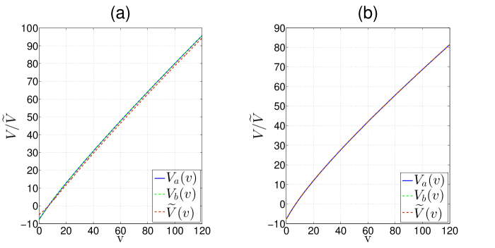
Figure 17: Numerical results for RNV advanced time coordinate as a function of the numerical $v$ coordinate. Panel (a) describes the case of two null fluids and panel (b) describes the mixed case. The initial ray RNV advanced time coordinate $V$ is evaluated in two methods, $V_{a}$ and $V_{b}$, and the horizon RNV advanced time coordinate $\widetilde{V}$ is evaluated by a single method ($b$). While the differences between $V_{a}$ and $V_{b}$ are extremely small in both cases (roundoff oriented, $\lesssim 10^{-14}$ in the case of two null fluids and $\lesssim 10^{-12}$ in the mixed case) the difference between $\widetilde{V}$ and $V$ is noticeable in the case of two null fluids (maximal difference is $|V-\widetilde{V}|\approx 2.9$) and small in the mixed case (maximal difference is $|V-\widetilde{V}|\approx 0.06$, although all three curves overlap in the scale of panel (b)).

A.2 Linear mass function derivation

We turn next to consider the specific ingoing null fluid stream defined by Eq. (15); we demonstrate that it has a linear contribution to the mass function $m(V)$ at late times. This property is gauge dependent and may vanish in a gauge transformation. We begin with a previous result of Poisson and Israel, [7]

$$m,_{a}=4\pi r^{2}T_{a}^{\>\,b}r,_{b}\,,$$

where $T_{ab}\equiv T_{\mu\nu}^{NF}$ is the energy-momentum tensor of the null fluid. We discuss here the ingoing null fluid stream on the initial ray $u=u_{0}$, so we are interested in finding $m,_{v}$. After the appropriate index lowering and submitting $g^{uv}=2e^{-\sigma}$, we obtain

$$m,_{v}=4\pi r^{2}g^{uv}T_{vv}^{NF}r,_{u}=-8\pi r^{2}e^{-\sigma}T_{vv}^{NF}r,_{u}\,.$$

Inserting the nonvanishing part of $T_{vv}^{NF}(u_{0},v)$ from Eq. (15) yields

$$m,_{v}(u_{0},v)=-8\pi A_{1}e^{-\sigma}(1-e^{r_{0}-r})^{2}\frac{1}{r,_{u}}\,.$$

We are interested in finding $m,_{V}=m,_{v}\frac{dv}{dV}$. We can see from Eq. (19) that $\frac{dv}{dV}=-2r,_{u}e^{-\sigma}$, so

$$m,_{V}(u_{0},V)=16\pi A_{1}e^{-2\sigma}(1-e^{r_{0}-r})^{2}\,.$$

Recalling that on our initial ray $\sigma(u_{0},v)=0$, we get the final result

$$m,_{V}(u_{0},V)=16\pi A_{1}(1-e^{r_{0}-r})^{2}\,.$$ (23)

The factor $(1-e^{r_{0}-r})^{2}$ approaches $1$ with the rise in $r$, yielding the required constant $m,_{V}$ (or linear $m(V)$). Fig. 18 displays the numerical $m,_{V}(V)$ and confirms that it fits the expected behavior.

Figure 18: Numerical results for $m,_{V}(V)$ on the initial ray $u_{0}=0$. The blue curve fits the single null fluid and two null fluids scenarios, which share the same ingoing null fluid stream, and the red curve fits the mixed case. In both cases $m,_{V}$ rises smoothly from zero and approaches a constant value, implying a linear mass function $m(V)$ at late times $(V\gtrsim 30)$.

References

- [1] R. Penrose, in Battelle Rencontres, edited by C. de Witt and J. Wheeler (W. A. Benjamin, New York, 1968), p. 222.
- [2] M. Simpson and R. Penrose, Internal instability in a Reissner-Nordström black hole, Int. J. Theor. Phys. 7, 183 (1973).
- [3] Y. Gursel, I. D. Novikov, V. D. Sandberg, and A. A. Starobinsky, Final state of the evolution of the interior of a charged black hole, Phys. Rev. D 20, 1260 (1979).
- [4] W. A. Hiscock, Evolution of the interior of a charged black hole, Phys. Lett. 83A, 110 (1981).
- [5] S. Chandrasekhar and J. B. Hartle, On crossing the Cauchy horizon of a Reissner-Nordström black hole, Proc. R. Soc. A 384, 301 (1982).
- [6] E. Poisson and W. Israel, Inner-Horizon Instability and Mass Inflation in Black Holes, Phys. Rev. Lett. 63, 1663 (1989).
- [7] E. Poisson and W. Israel, inner structure of black holes, Phys. Rev. D 41, 1796 (1990).
- [8] A. Ori, Inner Structure of a Charged Black Hole—An Exact Mass-Inflation Solution, Phys. Rev. Lett. 67, 789 (1991).
- [9] M. L. Gnedin and N. Y. Gnedin, Destruction of the Cauchy horizon in the Reissner-Nordström black hole, Classical Quantum Gravity 10, 1083 (1993).
- [10] P. R. Brady and J. D. Smith, Black Hole Singularities: A Numerical Approach, Phys. Rev. Lett. 75, 1256 (1995).
- [11] L. M. Burko, QED blue-sheet effects inside black holes, Phys. Rev. D 55, 2105 (1997).
- [12] L. M. Burko, Structure of the Black Hole’s Cauchy-Horizon Singularity, Phys. Rev. Lett. 79, 4958 (1997).
- [13] S. Hod and T. Piran, Mass Inflation in Dynamical Gravitational Collapse of a Charged Scalar Field, Phys. Rev. Lett. 81, 1554 (1998).
- [14] L. M. Burko and A. Ori, Analytic study of the null singularity inside spherical charged black holes, Phys. Rev. D 57, R7084 (1998).
- [15] L. M. Burko, Singularity deep inside the spherical charged black hole core, Phys. Rev. D 59, 024011 (1998).
- [16] L. M. Burko, Survival of the black hole’s Cauchy horizon under noncompact perturbations, Phys. Rev. D 66, 024046 (2002).
- [17] L. M. Burko, Black-Hole Singularities: A New Critical Phenomenon, Phys. Rev. Lett. 90, 121101 (2003).
- [18] M. Dafermos, Stability and instability of the Cauchy horizon for the spherically symmetric Einstein-Maxwell scalar field equations, Ann. Math. 158, 875 (2003).
- [19] A. Ori, Structure of the Singularity Inside a Realistic Rotating Black Hole, Phys. Rev. Lett. 68, 2117 (1992).
- [20] P. R. Brady, S. Droz, and S. M. Morsink, Late-time singularity inside nonspherical black holes, Phys. Rev. D 58, 084034 (1998).
- [21] A. Ori, Evolution of linear gravitational and electromagnetic perturbations inside a Kerr black hole, Phys. Rev. D 61, 024001 (1999).
- [22] A. Ori, Oscillatory Null Singularity inside Realistic Spinning Black Holes, Phys. Rev. Lett. 83, 5423 (1999).
- [23] A. J. S. Hamilton and G. Polhemus, Interior structure of rotating black holes. I. Concise derivation, Phys. Rev. D 84, 124055 (2011).
- [24] A. J. S. Hamilton, Interior structure of rotating black holes. II. Uncharged black holes, Phys. Rev. D 84, 124056 (2011).
- [25] A. J. S. Hamilton, Interior structure of rotating black holes. III. Charged black holes, Phys. Rev. D 84, 124057 (2011).
- [26] L. M. Burko, G. Khanna, and A. Zenginoğlu, Cauchy horizon singularity inside perturbed Kerr black holes, Phys. Rev. D 93, 041501(R) (2016).
- [27] P.C. Vaidya, The Gravitational Field of a Radiating Star, Proc. Indian Acad. Sci. A33, 264 (1951).
- [28] F. J. Tipler, Singularities in conformally at spacetimes, Phys. Lett. 64A, 8 (1977).
- [29] A. Ori, Strength of curvature singularities, Phys. Rev. D 61, 064016 (2000).
- [30] D. Marolf and A. Ori, Outgoing gravitational shock wave at the inner horizon: The late-time limit of black hole interiors, Phys. Rev. D 86, 124026 (2012).
- [31] E. Eilon and A. Ori, Numerical study of the gravitational shock wave inside a spherical charged black hole, Phys. Rev. D 94, 104060 (2016).
- [32] A. J. S. Hamilton and P. P. Avelino, The physics of the relativistic counterstreaming instability that drives mass inflation inside black holes, Phys. Rep. 495, 1 (2010).
- [33] E. Eilon and A. Ori, Adaptive gauge method for long-time double-null simulations of spherical black-hole spacetimes, Phys. Rev. D 93, 024016 (2016).
- [34] B. Waugh and K. Lake, Double-null coordinates for the Vaidya metric, Phys. Rev. D 34, 2978 (1986).
- [35] K. Lake and T. Zannias, Structure of singularities in the spherical gravitational collapse of a charged null fluid, Phys. Rev. D 43 , 1798 (1991) .
- [36] K. D. Patil, R. V. Saraykar, and S. H. Ghate, Strong curvature naked singularities in generalized Vaidya space-times, Pramana J. Phys. 52, 553 (1999).
- [37] A. Ori, (Unpublished), (1991).
- [38] D. N. Page, in Black Hole Physics, edited by V. De Sabbata and Z. Zhang, NATO Science Series 364 (Springer, NY, 1992), p. 185.
- [39] L. Dori, Non-Monotonous Singularity inside Spherically-Symmetric Black Holes, Master Thesis (2001), p. 35.
- [40] P. Abbott et al. (LIGO Scientific and Virgo Collaborations), Observation of Gravitational Waves from a Binary Black Hole Merger, Phys. Rev. Lett. 116, 061102 (2016).
- [41] P. Abbott et al. (Virgo and LIGO Scientific Collaborations), GW151226: Observation of Gravitational Waves from a 22- Solar-Mass Binary Black Hole Coalescence, Phys. Rev. Lett. 116, 241103 (2016).