Finding network communities using modularity density

Abstract

Many real-world complex networks exhibit a community structure, in which the modules correspond to actual functional units. Identifying these communities is a key challenge for scientists. A common approach is to search for the network partition that maximizes a quality function. Here, we present a detailed analysis of a recently proposed function, namely modularity density. We show that it does not incur in the drawbacks suffered by traditional modularity, and that it can identify networks without ground-truth community structure, deriving its analytical dependence on link density in generic random graphs. In addition, we show that modularity density allows an easy comparison between networks of different sizes, and we also present some limitations that methods based on modularity density may suffer from. Finally, we introduce an efficient, quadratic community detection algorithm based on modularity density maximization, validating its accuracy against theoretical predictions and on a set of benchmark networks.

Keywords: Complex Networks, Community Detection, Network Algorithms, Modularity Density

1 Introduction

The last two decades have seen an explosion in the study of complex systems, caused by the increasing relevance for society of such large interconnected structures, and by an unprecedented availability of data to analyze them. Many of these systems can be modelled as networks, in which the system elements are represented as nodes, and their interactions as connections, or edges, linking them [1, 2, 3]. The network representation of complex systems has been used in the social sciences [4, 5, 6, 7, 8], in biology [9, 10, 11, 12], and in studies of technological systems [13] and communication systems [14]. More recent work has focussed on the multilayer nature of complex networks, introducing a new framework that is particularly useful for the analysis of large complex data sets [15, 16]. Researchers have applied complex systems techniques to a wide range of disciplines, identifying and analyzing several defining features of complex networks, such as the small world property [17, 18, 19, 20], heterogeneous degree distributions [21, 22], clustering [23, 24], degree-degree correlations [25, 26], assortativity [27], synchronizability [28], and community structure [29]. Communities were originally studied in the context of social networks, in which they are formed by groups of people that share close friendship relations. However, communities of densely connected modules have been observed in several real-world and model networks of diverse nature [30, 31, 32, 33, 34, 35, 36, 37, 38, 39, 40, 41, 42], where, in general, they are defined as groups of nodes whose internal connections are denser or stronger than those that link nodes belonging to different groups. In all these cases, the presence of communities directly influences the behaviour of the system, where there is often a correspondence between communities and functional units. Ever since the discovery of community structure in real-world networks, a plethora of techniques devoted to their detection has been introduced [43, 44, 45, 46, 47, 48, 49, 50, 51]. The challenge is both theoretical, in proposing a good mathematical definition of what constitutes a community, and computational, in developing good heuristics that can detect communities in a reasonable time.

A common way of investigating the community structure of networks starts with the definition of a quality function, which assigns a score to any network partition. Larger scores correspond to better partitions, and algorithms are created to find the partition with the largest score. By far, the most common and used of such quality functions is modularity [52], that works by comparing the number of links inside each community to the number of links that would be expected if the nodes were connected at random, without any preference for links within or outside the community. A partition with a large modularity indicates that the communities have many internal links and few external ones, when compared to a randomized version of the network. However, despite its success, modularity also has some shortcomings, decreasing its general usefulness. In this Article, we study a new quality function, modularity density, that was originally introduced in [53, 54] and that has been shown to address the limitations of traditional modularity. We present a detailed analysis of its properties on synthetic networks typically used to evaluate quality functions, as well as on random graphs, which are a commonly used benchmark to test community detection methods. We also present some limitations that need to be taken into consideration when using methods based on modularity density. In addition, we describe a new community detection algorithm based on this metric, whose computational complexity is quadratic in the number of nodes, and validate it on synthetic and real-world networks, showing that it performs better that other currently available methods. Also, we argue that the nature of modularity density allows for a direct quantitative comparison of community structures across networks of different sizes.

2 Traditional modularity and its limitations

The modularity $Q$ of a network with $N$ nodes and $m$ links is defined as:

$$Q=\frac{1}{2m}\sum_{ij}\left(A_{ij}-\frac{k_{i}k_{j}}{2m}\right)\delta_{C_{i}C_{j}}\>,$$

where $A$ is the adjacency matrix of the network, $k_{i}$ is the degree of node $i$, $C_{i}$ is the community to which node $i$ is assigned and $\delta_{ij}$ is the Kronecker delta. The first term accounts for the presence or absence of a link between node $i$ and node $j$; the second term, instead, is the expected number of links between node $i$ and node $j$ in a random network with the same degree sequence as the original one.

A first limitation of modularity is that it is intrinsically dependent on the number and distribution of edges, rather than on the number of nodes. To see this, denote by $m_{C}$ and $e_{C}$ the number of internal and external links of community $C$, respectively. Moreover, let $k_{C}=2m_{C}+e_{C}$ be the sum of the degrees of the nodes in community $C$. With this notation, it is

$$Q=\sum_{C\in\mathcal{C}}\left[\frac{m_{C}}{m}-\left(\frac{k_{C}}{2m}\right)^{2}\right]\>,$$ (1)

where $\mathcal{C}=\left\{C_{1},C_{2},\ldots,C_{P}\right\}$ denotes the set of all communities in the partition. In this expression, each term in the sum refers to a different community. The first factor of each term corresponds to the internal density of links in the community, whereas the second factor encodes the expected density of links in the random network null model. Now, introduce the positive parameter $\alpha_{C}$, representing the ratio of external links to internal ones:

$$e_{C}=\alpha_{C}m_{C}\>.$$

The value of $\alpha_{C}$ is smaller for strong communitites, and higher for weaker ones. Then, we can write

$$Q=\sum_{C\in\mathcal{C}}\left[\frac{m_{C}}{m}-\left(\frac{2+\alpha_{C}}{2m}\right)^{2}m_{C}^{2}\right]\>.$$ (2)

From this expression, it is clear that a community $C$ gives a positive contribution to $Q$ only if:

$$m_{C}<\frac{4m}{(\alpha_{C}+2)^{2}}\>.$$

This implies that the condition for a community to give a positive contribution only depends on the number of edges in the community and on the total number of edges in the network, but not explicitly on the number of nodes.

A similar result can be obtained considering a network of $\kappa$ communities disconnected from each other, along the lines of [43]. Under the assumption that all groups have the same number of links, we can write

$$m_{C} =\frac{m}{\kappa}\>,$$

$$e_{C} =0\>,$$

$$k_{C} =\frac{2m}{\kappa}\>.$$

Then, from (1), it is

$$Q=\kappa\left[\frac{1}{m}\frac{m}{\kappa}-\left(\frac{1}{2m}\frac{2m}{\kappa}\right)^{2}\right]=1-\frac{1}{\kappa}\>.$$ (3)

This shows that modularity converges to 1 with the number of communities $\kappa$ regardless of the internal properties of the communities, such as their size, or the number of internal edges. As long as $\kappa$ is very large and all communities have the same number of edges ${}^{m}/{}_{\kappa}$, a network of disconnected trees has the same modularity of a network of disconnected cliques. As before, we also see that the number of nodes in each group does not explicitly contribute to $Q$, and, as an immediate consequence, a network composed of few cliques has a smaller modularity than a network composed of many disjoint trees.

In addition to these results, the effectiveness of modularity is not constant for all edge densities. To determine its dependence on this quantity, we follow [55] and connect the $\kappa$ groups in a ring configuration, where each community is linked with exactly one edge to the next one, and one edge to the previous one in the ring, for a total of $\kappa$ inter-community edges. In this scenario, we have

$$m_{C} =\frac{m}{\kappa}-1\>,$$

$$e_{C} =2\>,$$

$$k_{C} =\frac{2m}{\kappa}\>.$$

From (1), it follows that

$$Q=\kappa\left[\frac{1}{\kappa}-\frac{1}{m}-\left(\frac{1}{2m}\frac{2m}{\kappa}\right)^{2}\right]=1-\frac{\kappa}{m}-\frac{1}{\kappa}\>.$$

For constant $m$, this expression reaches its maximum when $\kappa=\sqrt{m}$, for which it is

$$Q=1-\frac{2}{\sqrt{m}}\>.$$

Thus, the highest modularity corresponds to a partition in $\sqrt{m}$ modules. Once again, the number of nodes in the communities does not affect its largest possible value. This major limitation of modularity is known as the resolution limit, and it indicates that modularity, as a quality function for community detection, has an intrinsic scale proportional to $\sqrt{m}$. The number and size of the communities that can be detected via modularity maximisation are bound to adhere to this limit, posing a serious question on the significance of results obtained with this method. In fact, in a more general framework, Fortunato and Barthélemy [55] have shown that, under some circumstances, the resolution limit can even force pairs of well-defined communities to be merged into a larger cluster, because this corresponds to a higher modularity.

Finally, it is worth noting that the trivial partition where all the nodes are put together in one single community, namely the whole network itself, has a modularity of 0. This can be easily seen from (2), since in this case the sum has only one term, $\alpha_{C}=0$ and $m_{C}=m$, so

$$Q=\frac{m}{m}-\frac{4m^{2}}{4m^{2}}=0\>.$$

At first, this might seem a desirable property for a quality function, since, intuitively, the trivial partition should not have a positive modularity. However, this implies that any partition that achieves a modularity larger than 0 is retained as a valid community structure. Since community detection algorithms try to maximize modularity, it is often the case that such a positive value can be found even on Erdős-Rényi random graphs [50]. To stress this point, the trivial partition with $Q=0$ can always be considered, but since one is interested in the maximum value of $Q$, it is often discarded in favour of a clustering that achieves any positive value of modularity. This poses a serious limitation to the ability of modularity-based algorithms to partition random graphs correctly.

Several variants of modularity have been proposed to address the resolution limit. For instance, multi-resolution methods, such as the one described in [56], introduce an additional tunable parameter $\eta>0$ in the expression for $Q$:

$$Q_{\eta}=\sum_{C\in\mathcal{C}}\left[\frac{m_{C}}{m}-\eta\left(\frac{k_{C}}{2m}\right)^{2}\right]\>.$$

Larger values of $\eta$ cause $Q_{\eta}$ to be larger for partitions with smaller modules, whereas smaller values favour larger communities. However, this approach suffers from similar limitations to those presented by the original modularity [57]. In particular, $Q_{\eta}$ has two contrasting behaviours: small clusters tend to be merged together, while large communities tend to be split into subgroups. Networks in which all the communities are of comparable size are immune to this problem, and one can find a value of $\eta$ for which they can all be resolved. However, the existence of an optimal $\eta$ is not guaranteed in the general case. In particular, for networks whose community sizes are heterogeneously distributed, e.g., following a power law, it is not possible to find a value of $\eta$ that avoids both problems. The reason for this is that the nature of the resolution limit is more general than the specific definitions of modularity and its multi-resolution extension. Several quality functions for community detection, including the one just mentioned, can be derived within the general framework of a first principle Potts model with Hamiltonian

$$H=-\sum_{ij}\left[a_{ij}A_{ij}-b_{ij}\left(1-A_{ij}\right)\right]\delta_{C_{i}C_{j}}\>,$$

where $a_{ij}$ and $b_{ij}$ are non-negative weights. Different choices for the weights result in different quality functions. However, only those using non-local weights can be truly free from the resolution limit [58], while all others, including modularity, multi-resolution modularity and functions based on quantities such as betweenness, shortest paths, triangles and loops, can never avoid it.

3 Modularity density

Recently, a new quality function called modularity density has been proposed to overcome the issues outlined above [53, 54]. Given a network partition, modularity density is defined as

$$Q_{ds}=\sum_{C\in\mathcal{C}}\left\{\frac{2m_{C}^{2}}{mn_{C}\left(n_{C}-1\right)}-\left[\frac{2m_{C}+e_{C}}{2m}\frac{2m_{C}}{n_{C}\left(n_{C}-1\right)}\right]^{2}-\sum_{\widetilde{C}≠C}\frac{m_{C\widetilde{C}}^{2}}{2mn_{C}n_{\widetilde{C}}}\right\}\>,$$ (4)

where $n_{C}$ is the number of nodes in community $C$, the internal sum is over all communities different from $C$, and $m_{C\widetilde{C}}$ is the number of edges between community $C$ and community $\widetilde{C}$. This new metric brings two major improvements over traditional modularity. First, it contains an explicit penalty for edges connecting nodes in different communities. This addresses the problem of the splitting of large communities, since each split introduces external links and is thus penalized. Second, all terms, including the penalty for inter-community edges, are explicitly weighted by the community sizes. Therefore, a partition with many edges linking two small communities is penalized more than one with the same number of edges linking two large ones. Thus, modularity density introduces local dependencies that are not found in traditional of modularity. Additionally, it is not related to the Potts model Hamiltonian, thus avoiding the resolution limit problem. Note that (4) requires $n_{C}>1$, which implies that partitions with communities consisting of an isolated node are not allowed.

To investigate the properties of modularity density in more depth, rewrite the expression for $Q_{ds}$ as

$$Q_{ds}=\sum_{C\in\mathcal{C}}\left[\frac{m_{C}}{m}p_{C}-\left(\frac{2m_{C}+e_{C}}{2m}p_{C}\right)^{2}-\sum_{\widetilde{C}≠C}\frac{m_{C\widetilde{C}}^{2}}{2mn_{C}n_{\widetilde{C}}}\right]\>,$$ (5)

where

$$p_{C}=\frac{2m_{C}}{n_{C}\left(n_{C}-1\right)}\>.$$

The parameter $p_{C}$ can assume values between 0 and 1, since it is the fraction of possible internal links actually present in community $C$. Thus, it measures the connection density of the community, or, equivalently, the probability that two random nodes inside $C$ are connected. From (5) it is clear that having many internal edges is not enough for a community to give a large contribution to modularity density. In fact, a strong community is one where the density of edges, rather than their number, is large. This also agrees with the intuitive notion that a community is a group of nodes that are densely connected amongst each other. Thus, a good partition is one that is characterized at the same time by a large number of intra-community links and a high density of edges within the communities. Modularity density achieves this by accounting for the number of nodes in each group and, in this sense, it has a more natural dependence on the local properties of the network and of the partition under consideration than does traditional modularity.

Next, it is instructive to study the behaviour of modularity density in the same cases described in the previous section. First, consider a network partitioned in just two communities, $C$ and $\widetilde{C}$. The contribution to $Q_{ds}$ of community $C$ is:

$$Q_{ds}^{C}=\frac{m_{C}}{m}p_{C}-\left(\frac{2m_{C}+e_{C}}{2m}p_{C}\right)^{2}-\frac{m_{C\widetilde{C}}^{2}}{2mn_{C}n_{\widetilde{C}}}\>.$$

Introducing the proportionality constant $\alpha_{C}$ as before, it is

$$Q_{ds}^{C}=\frac{m_{C}}{m}\left[p_{C}-\frac{\left(2+\alpha_{C}\right)^{2}}{4m}p_{C}^{2}m_{C}-\frac{\alpha_{C}^{2}m_{C}}{2n_{C}\left(N-n_{C}\right)}\right]\>,$$

where we used $n_{\widetilde{C}}=N-n_{C}$ and $m_{C\widetilde{C}}=e_{C}$. Unlike what happens with traditional modularity, the contribution of a single community depends explicitly on the number of internal links and on the size of the community itself.

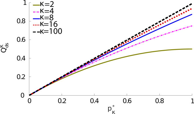
Figure 1: Modularity density increases with number of communities and their edge density. In networks composed of $\kappa$ disconnected modules, the modularity density $Q_{\mathrm{ds}}^{\kappa}$ depends only on $\kappa$ and the edge density of the communities $p_{\kappa}^{\star}$. Fixing one of the two parameters, $Q_{\mathrm{ds}}^{\kappa}$ always increases with the other.

Consider now again a network composed of $\kappa$ disjoint communities. Assuming that each community has the same number of nodes ${}^{N}/{}_{\kappa}$ and the same number of edges ${}^{m}/{}_{\kappa}$, the modularity density of such a network is:

$$Q_{ds}^{\kappa}=\kappa\left[\frac{p_{\kappa}^{\star}}{\kappa}-\left(\frac{p_{\kappa}^{\star}}{\kappa}\right)^{2}\right]=p_{\kappa}^{\star}\left(1-\frac{p_{\kappa}^{\star}}{\kappa}\right)\>,$$ (6)

where

$$p_{\kappa}^{\star}=\frac{2m}{N\left(\frac{N}{\kappa}-1\right)}$$

is the connection density of the communities. The first major difference between (3) and (6) is that $Q_{ds}^{\kappa}$ depends not only on the number of communities, but also on their density of edges, unlike traditional modularity, which only depends on $\kappa$. Also, for a fixed value of $\kappa$, $Q_{ds}^{\kappa}$ increases with $p_{\kappa}^{\star}$ (see figure 1). This is remarkable, since it indicates that the strength of the partition increases as more links are added within each group, in striking opposition with the behaviour of traditional modularity. We also note that for a fixed value of $p_{\kappa}^{\star}$, modularity density increases with the number of communities. Its theoretical maximum is reached in the limiting case of an infinite number of communities, with the special requirement that they are all cliques. Moreover, in one more substantial difference with traditional modularity, a network composed of few cliques in general has a higher modularity density than a network composed of an infinite number of sparse communities.

Finally, we study the test case of the ring of $\kappa$ communities each linked by a single edge to the next community and a single edge to the previous one. As before, it is $m_{C}={}^{m}/{}_{\kappa}-1$ and $e_{C}=2$, In addition, $m_{C\widetilde{C}}=1$ and $n_{C}={}^{N}/{}_{\kappa}$. Introducing the variables

$$\beta_{\kappa}=\frac{\frac{m}{\kappa}-1}{m}$$

and

$$p_{\kappa}^{\star}=\frac{2(\frac{m}{\kappa}-1)}{\frac{N}{\kappa}(\frac{N}{\kappa}-1)}\>,$$

we can write the modularity density as

$$Q_{ds}^{\mathrm{ring}}=\kappa\left[\beta_{\kappa}p_{\kappa}^{\star}-\left(\beta_{\kappa}+\frac{1}{m}\right)^{2}\left(p_{\kappa}^{\star}\right)^{2}-\frac{\kappa^{2}}{mN^{2}}\right]\>.$$ (7)

The optimal number of communities is the one that maximizes this expression, or, equivalently, the one for which its derivative vanishes. Differentiating $Q_{ds}^{\mathrm{ring}}$ with respect to $\kappa$, we obtain

$$\frac{\partial Q_{ds}^{\mathrm{ring}}}{\partial\kappa}=\kappa\beta_{\kappa}\partial_{\kappa}p_{\kappa}^{\star}-2\left(\beta_{\kappa}+\frac{1}{m}\right)p_{\kappa}^{\star}\partial_{\kappa}p_{\kappa}+\left(\beta_{\kappa}+\frac{1}{m}\right)^{2}(p_{\kappa}^{\star})^{2}+\left(\beta_{\kappa}-\frac{1}{\kappa}\right)p_{\kappa}-\frac{3\kappa^{2}}{mN^{2}}\>,$$

with

$$\partial_{\kappa}p_{\kappa}^{\star}=\frac{2\left(\kappa^{2}-2\kappa N+mN\right)}{N(\kappa-N)^{2}}\>.$$

This expression does not have a simple general root in terms of $\kappa$. Rather, the solutions depend on the local and global properties of the network. Thus, the number of groups does not seem to be constrained by an intrinsic scale of order $\sqrt{m}$.

As briefly discussed above, a major drawback of traditional modularity is that algorithms based on its maximization often find supposedly viable partitions on graphs with no ground-truth community structure. In such cases, the correct partition is either the one where all nodes are placed together, or the one with $N$ communities, each consisting of a single node. In either case, modularity vanishes. Thus, modularity-maximizing algorithms often suggest spurious community structures simply beause they have a non-zero modularity. Conversely, from (5) it follows that the one-group partition has a modularity density

$$Q_{ds}^{1}=p\left(1-p\right)\>,$$

where $p$ is the network density. Note that this expression is a parabola, whose roots are $p=0$ and $p=1$, which are the fully disconnected and fully connected graphs, respectively. Thus, a partition’s $Q_{ds}$ needs not only to be positive, but also to lie above the parabola for an algorithm based on modularity density maximization to accept it. We will see that this makes such algorithms not find communities on random graphs, as should be the case for a reliable community detection method.

4 A modularity density maximisation algorithm

Having discussed the advantages of modularity density as a quality function, we propose a community detection algorithm based on its maximization. Currently, the only published modularity density algorithm [54] is based on iterations of two steps, namely splitting and merging. The algorithm is divisive, starting from a partition where all the nodes are placed in a single community and then using bisections. Each splitting is performed using the Fiedler vector of the network, which is the eigenvector of the graph Laplacian corresponding to the second smallest eigenvalue. The graph Laplacian $L$ is defined as $L=D-A$, where $D$ is the diagonal matrix of the node degrees. The merging steps try to merge pairs of communities together if doing so improves the current partition. The two steps are repeated until the partition cannot be improved any longer, and the algorithm is deterministic, meaning that the same initial network always yields the same partition. Here, we extend and adapt an existing modularity maximisation algorithm, originally proposed in [50], which achieves the largest published scores of traditional modularity. Along the lines of the original method, our algorithm consists of four main steps, which we describe below. A contains a fully detailed discussion of the algorithm implementation and its computational complexity.

4.1 Bisection

In this step, we try to bisect the community under consideration (see figure 2A). To do so, we use the leading eigenvector of the modularity matrix. Despite suffering from the limitations discussed above, modularity still provides a good initial guess for a partition that is then refined by the subsequent steps.

4.2 Fine Tuning

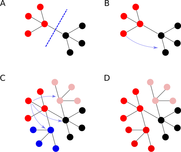
Figure 2: Schematic illustration of the algorithm steps. A) Bisection considers splitting a group of nodes into two separate communities. B) Fine tuning considers moving each node of a newly bisected group from its current community to the other. For example, it considers moving the red node to the black community. C) Final tuning considers moving each node of the network from its current community to any other existing community. For example, it considers moving the red node to the blue, the black and the pink communities. D) Agglomeration considers grouping two separate communities into a single one. For example, it considers grouping the red and blue nodes of panel C into a single red community.

After every bisection, the partition can be often improved by using a variant of the Kernighan-Lin algorithm [59]. We consider moving every node $i$ from the community into which it was assigned to the other (see figure 2B). Every such move would result in a change $\Delta Q_{ds}^{i}$ of the quality function, and we perform the move yielding the largest of such changes $\Delta_{\max}Q_{ds}^{i}$. Note that we introduce here a non-deterministic factor: given a tolerance parameter $\tau_{acc}$, we consider all moves achieving a change of modularity density within the interval $\left[\Delta_{\max}Q_{ds}^{i}-\tau_{acc},\Delta_{\max}Q_{ds}^{i}\right]$ to be equivalent. If more than one move falls within the acceptance interval, we randomly choose one to accept. This stochasticity allows the algorithm to explore the partition space without getting stuck on a local maximum, since it can accept moves that are not always optimal. Once a move has been performed, the corresponding node is flagged as blocked. Then, every non-blocked node is considered again and the procedure is repeated, until all nodes have been considered. At the completion of an iteration of this step, a decision tree is formed where each node of the tree represents a sequence of nodes in the network switching community, with an associated $\Delta Q_{ds}$ equal to the sum of all the changes in modularity density along the branches leading to the tree node. Then, we randomly choose a node in the decision tree amongst those achieving the largest positive increase in modularity density within an interval determined by the tolerance parameter $\tau_{acc}$, and perform all the moves corresponding to the chosen node. Finally, the whole step is repeated until no improvement in $Q_{ds}$ can be obtained.

4.3 Final Tuning

A further refinement of a current partition can be achieved by performing an additional tuning step. In the final tuning, we consider every node $i$ and try to move it to every other possible community $C$ already present in the partition (see figure 2C). The step is performed in a similar fashion to the fine tuning, repeatedly considering all the moves which result in an increase of modularity density in a small interval defined by the tolerance parameter $\tau_{acc}$ until all nodes have been moved. As before, we build a decision tree of partial switches and then perform all the moves up to the level in the tree that has been selected amongst those yielding the largest increase in $Q_{ds}$. We repeat this step until no further refinements can be found.

4.4 Agglomeration

A step that merges pairs of communities is fundamental. First of all, unlike both tuning steps, which are local because they only consider moving one node at a time, merging communities is a non-local step that allows one to better explore the landscape of modularity density [50]. For example, merging two entire communities can result in an increase of the quality function while partial mergers, i.e., moving only some nodes from one community to the other, could still have a lower score than the starting partition. Therefore, using only local moves, one could discard those partial mergers because they temporarily decrease the partition score, thus never achieving the beneficial complete merging of the two communities. In the case of modularity density, the agglomeration step is even more important, since no series of local moves could ever produce the full merging of two communities. This happens because modularity density does not allow communities of size 1. Thus, even if local steps had succeeded in moving all nodes except two from one community to another, any further move would be prohibited because it would result in a single-node community. This makes a global move essential for our algorithm. In the agglomeration step, we consider pairs of communities $C$ and $\widetilde{C}$ and try to merge them (see figure 2D). Each move results in a change in modularity density $\Delta Q_{ds}^{C,\widetilde{C}}$ and we randomly choose the move amongst those in the interval $\left[\Delta_{\max}Q_{ds}^{C,\widetilde{C}}-\tau_{acc},\Delta_{\max}Q_{ds}^{C,\widetilde{C}}\right]$, where $\Delta_{\max}Q_{ds}^{C,\widetilde{C}}$ is the largest increase in modularity density achieved by any move. We build a decision tree by progressively merging pairs of communities, until there is only a single community left. We then look at the nodes in the tree corresponding to the largest increase in modularity density but, in difference from the previous steps, if more than one node results in the same increase, we select the one with the smallest number of communities. The whole step is repeated until the current partition cannot be improved further.

4.5 Summary

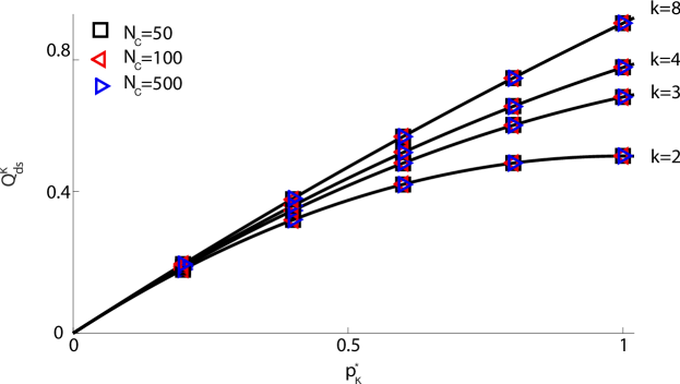
Figure 3: Modularity density for networks of $\kappa$ disconnected communities. The predictions of (6) (solid lines) are confirmed by numerical simulations throughout the range of $p_{\kappa}^{\star}$ and for different values of $\kappa$. For each $\kappa$, we consider groups with 50, 100 and 500 nodes, respectively. Additionally, and as expected, we observe that the value of modularity density does not depend on the number of nodes in each community, but only on the number of communities and their internal density. Each point is the average over 100 network realizations.

With these four steps, the algorithm can be summarized as:

• Start with a single community containing all nodes.

• Try to bisect the network using the leading eigenvector of the modularity matrix.

• If the bisection was successful, then perform a fine tuning step.

• Iterate the bisection and fine tuning steps on each of the communities in the current partition, until no further splitting and refinement can be performed.

• Perform the final tuning step.

• Perform the agglomeration step.

• Repeat the sequence of steps until it is no longer possible to find an increase in modularity density.

As described in detail in A, the worst-case computational complexity of the full algorithm is $O\left(N^{2}\right)$.

5 Validation

To validate our algorithm, we test it on several synthetic and real-world networks. First, we verify that it reproduces the theoretical predictions on networks of disconnected communities and on rings of modules, discussed in section 2 and section 3. Then, we analyze its behaviour on random networks belonging to different ensembles. Finally, we run it on a set of benchmark networks, comparing the results with the best ones currently published.

5.1 Disconnected communities and rings

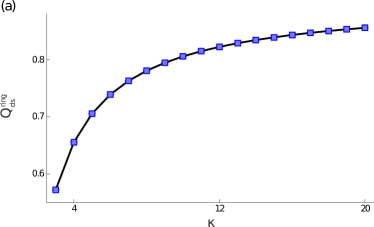
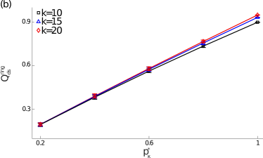
Figure 4: Modularity density for rings of communities. We simulate ring networks composed by with a varying number of communities $\kappa$ and compare the theoretical values of modularity density with the results of our algorithm. In panel (a) we consider networks of $\kappa$ fully connected cliques, finding a perfect agreement between theoretical value (solid line) and simulations (squares). In panel (b), we build networks with different fixed values of $\kappa$ and vary their internal density. Note that, differently from (a), here the groups are not fully connected. The theoretical values (lines) and simulation results match precisely. In both panels, each point is the average over 100 realizations of the same network.

First, we consider networks formed by $\kappa$ disconnected communities. Equation (6) indicates that the modularity density of such networks depends only on the connection probability $p^{\star}_{\kappa}$ and on $\kappa$ itself, but not on the size of each community. We find an exact agreement between the simulation results and the theoretical prediction for all the values of $\kappa$ (figure 3). We also note that the values of modularity density found in the simulations do not depend on the number of nodes in the communities.

As a second test, we simulate two types of ring networks of communities. We start by making the communities cliques of 5 fully connected nodes, and vary $\kappa$ from 3 to 20. From (7), the expected modularity density of these networks is

$$Q_{ds}^{\mathrm{ring}}=\kappa\left[\beta_{\kappa}-\left(\beta_{\kappa}+\frac{1}{m}\right)^{2}-\frac{\kappa^{2}}{25m}\right]\>.$$

The comparison between the modularity density predicted by this expression and the values obtained in our simulations is shown in figure 4(a). We find a precise agreement between the two, showing that our algorithm correctly identifies the cliques without splitting them, and finds the right value of modularity density. Next, we build ring networks in which we fix $\kappa$ and vary the community density $p_{\kappa}^{\star}$. Each community contains 50 nodes, and we vary $p_{\kappa}^{\star}$ from $0.2$ to 1, performin the test for $\kappa=10$, $\kappa=15$ and $\kappa=20$. The results, in figure 4(b), show a perfect agreement in all cases, again indicating that our algorithm correctly partitions the networks.

5.2 Random networks

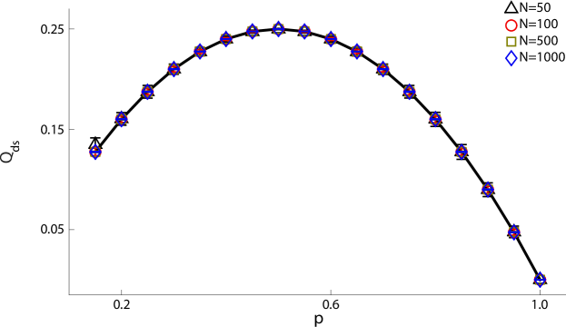
Figure 5: Modularity density on Erdős-Rényi graphs. We build ensembles of random networks, with different sizes and different densities, comparing the theoretical modularity density (solid line) and the one found by our algorithm. Up to finite-size effects for the smallest and least dense networks, we find a perfect agreement between theoretical prediction and simulation results, with all the results collapsing on the same curve. Each point is the average over 1000 realizations of the same network parameters.

As we argued in the previous sections, a desirable feature of a community detection algorithm is that it does not propose a complex partition of graphs without ground-truth community structure. To verify that our algorithm satisfies this requirement, we test it on Erdős-Rényi random graphs. For graphs in this ensemble, every possible edge between $N$ nodes exists independently with probability $p$. Thus, the average number of edges is $\frac{1}{2}Np\left(N-1\right)$. These networks do not have any true community structure, since all their edges are fully random, and thus they are one of the benchmarks against which community detection algorithms are often tested. For our simulations, we create networks with values of $p$ from $0.15$ to $0.90$ and number of nodes 50, 100, 500 and 1000. The results, in figure 5, show that for all network sizes, the average modularity density matches almost perfectly the theoretical prediction. Even for small networks, where finite-size effects are largest, the values lie in close proximity to the theoretical parabola and we can only observe a small deviation for the smallest networks at low values of $p$. Also note that all the results collapse on the theoretical curve, which does not depend on network size. These results represent a major improvement over modularity-based algorithms, that typically detect communities even on Erdős-Rényi networks. In addition, Erdős-Rényi networks are locally tree-like for low enough values of $p$, and highly clustered for $p$ close to 1. Thus, the results also indicate that modularity density is highly effective in detecting when no real communities exist in locally tree-like graphs, and does not introduce spurious modules even when the clustering increases. In fact, also the limiting case of fully connected graphs, which corresponds to a link probability $p$ identically equal to 1, is properly identified by our method.

As a special case of random networks, we also study random regular graphs. Random regular graphs are random networks where all nodes have the same degree, but the edges are still randomly placed. Using the algorithm described in Ref. [60], we create random regular graphs with 100, 500 and 1000 nodes. For each of the three network sizes, we consider degrees ranging from 4 to 20, 100 and 500, respectively. For every pair of size and degree, we generate 100 network realizations, on which we run our community detection algorithm. The results, depicted in figure 6, show a good agreement between theoretical predictions and simulations. The only exceptions are three cases that correspond to the sparsest graph of each given size.

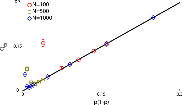
Figure 6: Modularity density on random regular graphs. We build ensembles of random regular networks, with different sizes and degree, comparing the theoretical modularity density (solid line) and the one found by our algorithm. With the exception of the sparsest network for each size, we find a good agreement between theoretical prediction and simulation results, with all the results collapsing on the same curve. Each point is the average over 100 realizations of the same network parameters.

These results show one of the major strengths of modularity density. However, it is well known that most real-world networks are not well represented by Erdős-Rényi graphs or random regular graphs. Rather, they are characterized by heterogeneous degree distributions. Thus, to further verify the performance of our algorithm, we test it on LFR networks [44]. These constitute a set of widely-used benchmark networks, whose distributions of degrees and community sizes follow a power-law $P\left(k\right)\sim k^{-\gamma}$. For our tests, we fix the network size to $N=500$ and vary the other parameters, namely the exponent $\gamma$ of the degree distribution, the mean degree $\left\langle k\right\rangle$ and the largest degree $k_{\max}$. Also, we ensure that the networks thus created contain a single community, so that no actual community structure is present. We run our algorithm on the networks thus generated and compare its results with the theoretical expectations. The results, presented in figure 7, show that for $\gamma=2.5$ and $\gamma=3$, the modularity density found by the algorithm closely follows the predicted value for networks of all densities. We do observe, however, some deviations from the predicted values at $\gamma=2$. This is probably due to the fact that, asymptotically, no networks exist with a pure power-law degree distribution for $\gamma<2$ [22]. Thus, in the limit of $\gamma=2$, and particularly for low densities, a spurious structure of stars with bridges appears, effectively introducing communities in the networks.

5.3 Benchmark networks

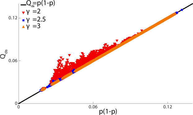
Figure 7: Modularity density for LFR networks. We run our algorithm on random LFR networks without community structure, with $N=500$ nodes and varying parameters. In particular, we let the mean degree $\left\langle k\right\rangle$ assume the values 15, 25, 35, 44 and 55, and the largest degree $k_{\max}$ be 150, 200 and 250. For each combination of the parameters, we generate 100 networks and for each we record the edge density $p$ and the largest modularity density our algorithm finds. The plot shows considerable agreement between the theoretical modularity density (solid line) and the one found by the algorithm. The only deviations appear for $\gamma=2$ and low $p$, and they are probably due to the breakdown of the LFR model for this limiting value of the degree distribution exponent.

We now verify the performance of our algorithm on some well known networks, for which results of the maximum modularity density obtained so far are available. The first is Zachary’s Karate Club network [61]. This is a friendship network between 34 members of a karate club in a U.S. university during the 1970s and it has become one of the most standard benchmarks to test community detection algorithms. The interest in this network lies in the fact that, not long after it was recorded, the club split into two subgroups due to internal problems between two members, namely the manager and the coach. Thus, a traditional challenge is to be able to detect these two groups based only on the friendship data available in the network topology, under the assumption that the members would decide to follow whichever leader they were more strongly related to between the coach and the manager. Of the 561 possible edges in the network, only 78 of them are present, making the network fairly sparse, with an effective connection probability $p\approx 0.139$.

A second benchmark network we consider is the American College Football Club network [29]. Here, the nodes represent different college football clubs and an edge connects two teams if there has been a regular-season game between them during the 2000 season. This network is known to have a natural community structure because the teams are divided into different leagues, thus making matches between teams more or less likely depending on the group they belong to.

Table 1: Accuracy validation. The comparison between the published results and the ones obtained with our algorithm on real-world and synthetic benchmark networks shows that our algorithm always performs better than the current best one. Note that currently this is the only other algorithm based on modularity density maximisation. All the already published results are found in [54].

• Benchmark	$Q_{ds}$	$Q_{ds,pub}$	$p$	$p(1-p)$
  Karate Club	$0.235$	$0.231$	$0.139$	$0.120$
  Football Club	$0.490931$	$0.4909$	$0.0935$	$0.0848$
  LFR, $\mu=0.05$	$0.5220\pm 0.0039$	$0.4979$	$0.0156\pm 0.0001$	$0.0154\pm 0.0001$
  LFR, $\mu=0.10$	$0.4638\pm 0.0033$	$0.4522$	$0.0154\pm 0.0001$	$0.0152\pm 0.0001$
  LFR, $\mu=0.15$	$0.4249\pm 0.0030$	$0.4013$	$0.0157\pm 0.0002$	$0.0155\pm 0.0002$
  LFR, $\mu=0.20$	$0.3982\pm 0.0054$	$0.384$	$0.0156\pm 0.0001$	$0.0154\pm 0.0001$
  LFR, $\mu=0.25$	$0.3465\pm 0.0085$	$0.3347$	$0.0156\pm 0.0001$	$0.0154\pm 0.0001$
  LFR, $\mu=0.30$	$0.2986\pm 0.0034$	$0.2619$	$0.0156\pm 0.0001$	$0.0154\pm 0.0001$
  LFR, $\mu=0.35$	$0.2546\pm 0.0101$	$0.2377$	$0.0156\pm 0.0001$	$0.0154\pm 0.0001$
  LFR, $\mu=0.40$	$0.2340\pm 0.0069$	$0.199$	$0.0156\pm 0.0001$	$0.0154\pm 0.0001$
  LFR, $\mu=0.45$	$0.2029\pm 0.0064$	$0.169$	$0.0156\pm 0.0001$	$0.0154\pm 0.0001$
  LFR, $\mu=0.50$	$0.1579\pm 0.0027$	$0.1385$	$0.0156\pm 0.0001$	$0.0154\pm 0.0001$

Finally, we consider again some LFR benchmark networks, choosing a set of parameters for which already published results exist. Table 1 presents a comparison between the results obtained using our algorithm and the best results available in the literature. Note that currently there is only one other algorithm based on modularity density. Because of the stochasticity within our method, for each value of the mixing parameter $\mu$, we create 10 realizations of the network and run the algorithm 100 times on each, reporting the average maximum modularity density found. In all cases considered, our algorithm finds a partition with higher modularity density than the best one currently published.

6 Limitations

So far, we have shown that our algorithm identifies the correct value of modularity density on a range of test networks. However, it is also worth noting that methods based on modularity density present some limitations in special cases.

To show this, we analyze regular ring lattice networks. These are graphs composed by a ring of $N$ nodes, each connected to a number of neighbours in each direction. We consider networks of 100, 500 and 1000 nodes, for which the number of neighbours of each node varies from 8 to 40, 200 and 500, respectively. The results, depicted in figure 8, illustrate how the theoretical prediction and the simulated results differ on almost all cases considered. In fact, with one exception, there is always a set of communities with a higher value of modularity density than the one corresponding to the trivial partition.

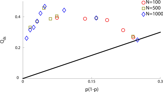
Figure 8: Modularity density on regular ring lattice graphs. We build regular ring lattice graphs, with different sizes and degrees, comparing the theoretical modularity density (solid line) and the one found by our algorithm. The results show that ring lattices are a limitation of modularity density. In fact, in almost all cases it is possible to find a network partition with a higher modularity density than the trivial one, corresponding to the absence of ground-truth communities.

Trees are another special case where modularity density exhibits some shortcomings. To see this, consider a tree with $N$ nodes. If all the nodes are put in a single community, the modularity density is given by:

$$Q^{(1)}_{ds}=p(1-p)=\frac{2(N-2)}{N^{2}}$$

If instead one divides the nodes between two different communities of equal size and equal number of internal links, it is

$$Q^{(2)}_{ds}=\frac{4(1+(N-4)N)}{N^{2}(N-1)}\>,$$

where we used the fact that, for a tree, there can only be one link between the two communities if they do not consist of disconnected components. It follows that, for $N\geqslant 6$, $Q^{(2)}_{ds}>Q^{(1)}_{ds}$, that is, for trees with more than 6 nodes, a partition in two equally sized communities always has a larger modularity density than the trivial partition. More generally, partitions with a larger number of equally sized communities tend to have a larger score, as can be seen in figure 9.

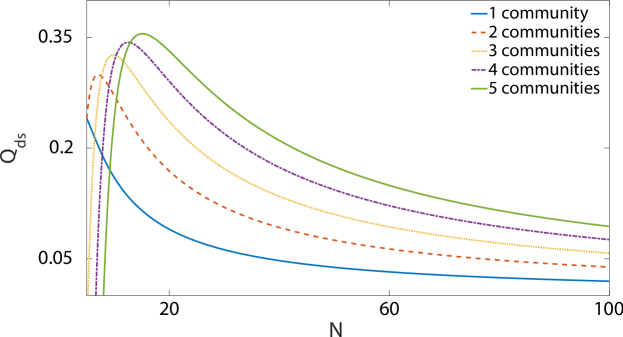
Figure 9: Modularity density for random trees partitioned into equally sized communities. The values indicate that trees constitute a limitation to the application of modularity density, since, for more than 6 nodes, partitions with more than one community always have larger modularity density than the trivial one.

7 Conclusions

Communities are a fundamental structure that is often present in real-world complex networks. Thus, the ability to accurately and efficiently detect them is of great relevance to the analysis of complex data sets. Despite their success, traditional methods based on modularity have been shown to suffer from limitations. We have presented a detailed analysis of the properties of modularity density, an alternative quality function for community detection, showing that it does not suffer from the drawbacks that affect traditional modularity. In particular, modularity density does not depend separately on the size of the network or the number of edges, but only on the combination of these two properties in terms of the density of links within the communities. As a consequence, it allows a direct quantitative comparison of the community structure across networks of different sizes and number of edges. At the light of these considerations, we have introduced a new community detection algorithm based on modularity density maximization. Investigating its performance on Erdős-Rényi and heterogeneous random networks, we showed that it correctly identifies them as containing no actual communities. Moreover, our algorithm outperforms the other existing modularity-density-based method on every benchmark network that we tested. The high level of accuracy it reaches, its low computational complexity, and the ability to properly identify networks with no ground-truth communities make it a powerful tool to investigate complex systems and extract meaningful information from the network representation of large data sets, giving it a broad range of application throughout the physical sciences. At the same time, we have also identified some limitations of modularity density that were not previously known. More specifically, we found that the theoretical maximum of modularity density for ring lattices and pure random trees does not correspond to the trivial partition, but rather to partitions with more than one community. We find this particularly intriguing, since Erdős-Rényi graphs are locally tree-like. Thus, these results seem to suggest a certain relevance of long-distance links for a correct behaviour of modularity density. Since most real-world networks are not pure trees or ring lattices, and indeed do feature shortcut links, we believe these limitations do not affect the suitability of modularity density and methods based on it in the analysis and modelling of complex systems. We will further investigate these limitations in future work. Additionally, we will also extend this method to other types of networks, such as bipartite graphs, which require a redefinition of the concept of community itself.

An implementation of our algorithm is freely available for download at www.fedebotta.com.

Appendix A Implementation details

Here, we provide a detailed description of the implementation of the algorithm presented above. To describe how the different steps are carried out, first we introduce some notation. Let $P=\left|\mathcal{C}\right|$ be the size of the current partition. Then, let $M$ be the partition adjacency matrix of the network, i.e., the $P\times P$ matrix whose elements $m_{C\widetilde{C}}$ are the number of links between community $C$ and community $\widetilde{C}$. Also, let $X$ be the community spectra matrix, i.e., the $N\times P$ matrix whose elements $x_{iC}$ are the number of links between node $i$ and nodes in community $C$. Finally, let $\mathbf{S}$ be the $P$-dimensional community size vector, whose elements are the sizes of the communities.

Note that our implementation uses three tolerance parameters:

1. Power method tolerance $\tau_{pwm}$. This parameter determines the tolerance for the floating-point comparisons in the power method.

2. Bisection tolerance $\tau_{bs}$. Since a bisection with the leading eigenvector of the classical modularity matrix does not guarantee an increase in modularity density, we introduce a tolerance $\tau_{bs}$. After each bisection, we check the difference between the new and old values of modularity density. A bisection is accepted if modularity density increases or if it decreases by an amount smaller than $\tau_{bs}$ (more details are given in A.1).

3. Acceptance tolerance $\tau_{acc}$. This parameter defines the size of the tolerance range when finding the moves that maximally increase modularity density during tuning and agglomeration steps.

A.1 Bisection

The first step in the algorithm attempts to bisect a community (see also figure 2A), which can be either the whole network or a previously determined community, using the traditional modularity matrix. To do so, we use the spectral method, which we briefly review here. The modularity matrix $B$ is defined as

$$B=A_{ij}-\frac{k_{i}k_{j}}{2m}\>,$$

and the expression for the modularity of a given partition is

$$Q=\frac{1}{2m}\sum_{ij}B_{ij}\delta_{C_{i}C_{j}}\>.$$ (8)

Since we are only considering a potential bisection, $C_{i}$ can only assume two values. Thus, a partition can be represented by a vector $\mathbf{s}$ whose entries $s_{i}$ are $1$ and $-1$ if node $i$ is assigned to the first or the second community resulting from the split, respectively. Then, substituting the expression

$$\delta_{C_{i}C_{j}}=\frac{1}{2}(s_{i}s_{j}+1)$$

in (8), it is

$$Q=\frac{1}{4m}\sum_{ij}B_{ij}s_{i}s_{j}\>.$$

The vector $\mathbf{s}$ can be expressed in terms of the normalized eigenvectors of $B$ as

$$\mathbf{s}=\sum_{i=1}^{N}\vartheta_{i}\mathbf{v}_{i}\>,$$

where the $\vartheta$ are linear combination coefficients, and $\mathbf{v}_{i}$ is the $i^{\mathrm{th}}$ eigenvector of the modularity matrix, corresponding to the eigenvalue $\lambda_{i}$. substituting in (8), we obtain

$$Q=\frac{1}{4m}\sum_{i=1}^{N}\vartheta_{i}^{2}\lambda_{i}\>.$$

If we label the eigenvalues so that $\lambda_{1}>\lambda_{2}>\cdots>\lambda_{N}$, this expression is maximized when $\mathbf{s}$ is parallel to the leading eigenvector $\mathbf{v}_{1}$. However, $\mathbf{s}$ is a vector whose entries can only be ±1. Thus, we can only choose its elements to make it as parallel to $\mathbf{v}_{1}$ as possible. One way of achieving this is to set $s_{i}=1$ if ${v_{1}}_{i}>0$ and $s_{i}=-1$ if ${v_{1}}_{i}<0$. Then, the bisection consists in finding the leading eigenvector of $B$ and, if the corresponding eigenvalue is positive, dividing the nodes according to this rule. Several metohds can be used to diagonalize $B$. Since we only need to find a single eigenvector, and this step only provides a starting guess, we choose to use the power method, which offers a good tradeoff between speed and accuracy.

Further consideration must be given to the fact that we are performing a bisection based on the modularity matrix, whereas our aim is to maximize modularity density. The potential problem is that a bisection based on modularity might not result in a larger value of modularity density. To avoid this, we introduce a tolerance parameter $\tau_{bs}$, whose role is to determine the largest possible decrease in modularity density that we want to accept when bisecting. In other words, if after the bisection the modularity density of the new partition has decreased by a value larger than $\tau_{bs}$, we do not accept the split, and keep the original partition. We consider only one exception to this rule, namely the first iteration of the bisection. At the start of the algorithm, all nodes are placed together and we try to bisect the whole network. At this point, we accept any bisection in order to allow at least a whole iteration of the whole algorithm. Indeed, if we didn’t accept that, both the tuning and agglomeration steps could not be executed, thus leaving the network not partitioned. Note that not partitioning the network could be the correct answer, but we want to make sure that we have considered other partitions as well at least once. If not partitioning the network is the best answer, this will be found by the agglomeration step, that will merge all the communities together.

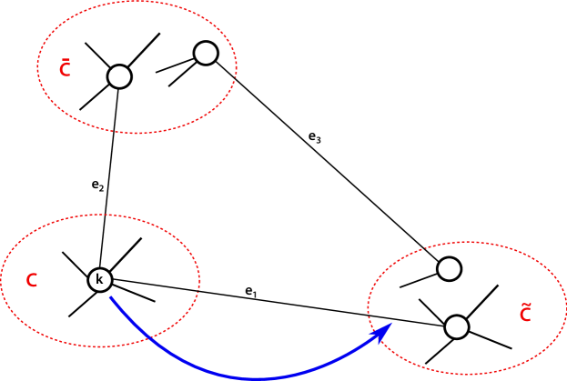
Figure 10: Schematic illustration of node $i$ moving from community $C$ to community $\widetilde{C}$.

Finally, we note that the previous expression for $B$ is correct only when considering the whole network. When trying to partition a single community $C$ which does not contain all the nodes, we need to construct an $n_{C}\times n_{C}$ sub-modularity matrix $B^{C}$ whose elements are

$$B^{C}_{ij}=A_{ij}-\frac{k_{i}k_{j}}{2m}-\delta_{ij}\left(k_{i}^{C}-k_{i}\frac{k_{C}}{2m}\right)\>,$$

where $k_{i}^{C}$ is the degree of node $i$ within the community $C$. Using this matrix, we then perform the bisection step as described above.

In Algorithm 1, we present a detailed description of the implementation of this step. For each community, the computation of the leading eigenvalue through the power method requires $O\left(m_{c}n_{c}\right)$ steps. Thus, the worst-case complexity of the the bisection step is $O\left(mN\right)$.

Algorithm 1
Pseudocode for the bisection step.

1:procedure Bisection Step

2:     flag first bisection $\leftarrow$ 1 $\triangleright$ flag that this is the first bisection

3:     $w\leftarrow 1$ $\triangleright$ $w$ is the community under consideration

4:     $|S|\leftarrow$ 1 $\triangleright$ Current number of communities

5:     while $w\leq$ $|S|$ do

6:         current number of nodes $\leftarrow S[w]$ $\triangleright$ $S$ is the community size vector

7:         current nodes labels $\leftarrow$ find nodes in $S[w]$

8:         $B\leftarrow$ construct $B$ $\triangleright$ $B$ is modularity matrix of the current nodes

9:         if current number of nodes $>$ 2 then

10:              leading $\lambda$, leading $v$ $\leftarrow$ power method(B)

11:         end if

12:         if $v$ has at least two negative and two positive components then

13:              flag bisection $\leftarrow 1$

14:         end if

15:         if $\lambda>0\leavevmode\nobreak\ \&$ flag bisection then

16:              bisection($v$, current nodes labels, current number of nodes)

17:              $|S|\leftarrow|S|+1$

18:              if old $Q_{ds}-$ new $Q_{ds}>\tau_{bs}$ and flag first bisection$=0$ then

19:                  cancel bisection

20:                  flag$[w]\leftarrow 1$

21:                  flag fine tuning $\leftarrow$ 0

22:              end if

23:              if $S[w]>2$ or $S[w+1]>2]$ and flag fine tuning then

24:                  fine tuning(current number of nodes, current nodes labels)

25:              end if

26:              flag first bisection $\leftarrow$ 0

27:         else

28:             flag$[w]\leftarrow 1$ $\triangleright$ Flag $w$ as blocked

29:         end if

30:         flag fine tuning $\leftarrow$ 1

31:         if flag$[w]$ then

32:             $w\leftarrow w+1$

33:         end if

34:     end while

35:end procedure

A.2 Tuning Steps

The crucial part of both the fine tuning and final tuning steps is that they try to move individual nodes to different communities (see also figure 2B and C). Thus, we need to consider what happens to the current partition and how $M$, $X$ and $\mathbf{S}$ change when we move a node $i$ from community $C$ to community $\widetilde{C}$. Figure 10 provides an intuitive scheme to illustrate the changes that follow from such a move. In general, both the number of internal and external links of $C$ will change, since node $i$ is leaving this community. However, to correctly update the modularity density, we also need to keep track of the changes in all the specific numbers of links between $C$ and every other community in the current partition. Similarly, we need to ensure that the internal and external links of $\widetilde{C}$ are updated correctly. Finally, the sizes of the two communities changes as well as a consequence of the move. Below, we describe how to efficiently perform these updates.

A.2.1 Updating the Partition Adjacency Matrix

The partition adjacency matrix $M$ keeps track of the number of edges between each pair of communities, as well as the internal number of edges of each community in its diagonal elements. Looking at figure 10, one can see that the following quantities change:

• The number of internal links of the community $C$ that node $i$ is leaving decreases by the internal degree of node $i$, which is the number of links it has to other nodes in $C$.

• The number of internal links of the community $\widetilde{C}$ that node $i$ is moving to increases by the number of links node $i$ has with other nodes in $\widetilde{C}$.

• The number of links between the old and the new community of node $i$ increases by the number of links between $i$ and its old community, and decreases by the number of links between $i$ and its new community.

• The number of links between the old community $C$ and all the other communities $\bar{C}\notin\left\{C,\widetilde{C}\right\}$ decreases by the number of links between $i$ and nodes in $\bar{C}$.

• The number of links between the new community $\widetilde{C}$ and all the other communities $\bar{C}\notin\left\{C,\widetilde{C}\right\}$ increases by the number of links between $i$ and nodes in $\bar{C}$.

In formulae:

$$m_{C} \to m_{C}-x_{iC}$$

$$m_{\widetilde{C}} \to m_{\widetilde{C}}+x_{i\widetilde{C}}$$

$$m_{C\widetilde{C}} \to m_{C\widetilde{C}}+x_{iC}-x_{i\widetilde{C}}$$

$$m_{C\bar{C}} \to m_{C\bar{C}}-x_{i\bar{C}}\quad\quad\quad\quad\forall\bar{C}\notin\left\{C,\widetilde{C}\right\}$$

$$m_{\widetilde{C}\bar{C}} \to m_{\widetilde{C}\bar{C}}+x_{i\bar{C}}\quad\quad\quad\quad\forall\bar{C}\notin\left\{C,\widetilde{C}\right\}\>,$$

where we dropped the repeated index for the diagonal elements of $M$ to keep the notation consistent.

A.2.2 Updating the Community Spectra Matrix

The rows of the matrix $X$ are the community spectra of the nodes, containing the numbers of links that each node forms with nodes in all the individual communities in the current partition. When a node $i$ changes community, its community spectrum does not change. However, every neighbour of $i$ will experience a change in the number of connections it has to nodes in the old and new communities of $i$. In particular, in moving node $i$ from $C$ to $\widetilde{C}$, the following changes happen:

• Since $i$ is no longer in community $C$, all the nodes connected to $i$ have one link less to $C$.

• Since $i$ is now in community $\widetilde{C}$, all the nodes connected to $i$ have one connection more to $\widetilde{C}$.

In formulae:

$$x_{lC} \to x_{lC}-1 \quad\forall l\mid A_{il}=1$$

$$x_{l\widetilde{C}} \to x_{l\widetilde{C}}+1 \quad\forall l\mid A_{il}=1\>.$$

A.2.3 Updating the Community Size Vector

The updates to this vector are straightforward:

$$S_{C} \to n_{C}-1$$

$$S_{\widetilde{C}} \to n_{\widetilde{C}}+1\>.$$

A.2.4 Change in Modularity Density

Algorithm 2
Pseudocode for the fine tuning step.

1:procedure Fine Tuning Step

2:     flag increase $\leftarrow$ 1 $\triangleright$ Flag if there is an increase in modularity density

3:     while flag increase do

4:         flag increase $\leftarrow$ 0 $\triangleright$ Reset the flag

5:         for $i_{1}<$ current number of nodes do

6:              for $i_{2}<$ current number of nodes do

7:                  if flag node$[i_{2}]=0$ then $\triangleright$ if node $i_{2}$ is not blocked

8:                       if $x_{i_{2},\widetilde{C}}>0$ then

9:                           $\Delta Q_{ds}[i_{2}]\leftarrow$ change in $Q_{ds}$ if $i_{2}$ changes community

10:                       end if

11:                  end if

12:              end for

13:              $\max\Delta Q_{ds}\leftarrow$ maximum increase in $Q_{ds}$

14:              find all nodes within $\tau_{acc}$ from $\max\Delta Q_{ds}$

15:              node to move $\leftarrow$ pick randomly between nodes with $\max\Delta Q_{ds}$

16:              flag node$[$node to move$]\leftarrow$ 1

17:              fine tuning tree$[i_{1}]\leftarrow$ fine tuning tree$[i_{1}-1]+\max\Delta Q_{ds}$

18:         end for

19:         $\max\Delta Q_{ds}\leftarrow\max($ fine tuning tree$)$

20:         if $\max\Delta Q_{ds}>$ 0 then

21:              find all steps within $\tau_{acc}$ of $\max\Delta Q_{ds}$

22:              step in fine tuning tree $\leftarrow$ pick randomly step with $\max\Delta Q_{ds}$

23:              perform all updates in fine tuning tree until the chosen step

24:              flag increase $\leftarrow 1$

25:         end if

26:     end while

27:end procedure

Since $Q_{ds}$ is defined as a sum over all current communities, we consider the terms in its expression (4) separately, and show how they change when node $i$ moves from community $C$ to community $\widetilde{C}$. We first look at what happens to the contributions of a community $\bar{C}$ different from $C$ and $\widetilde{C}$. In this case, the only changes happen for two terms in the internal sum:

$$\sum_{\hat{C}\neq\bar{C}}\frac{m_{\bar{C}\hat{C}}^{2}}{2mn_{\bar{C}}n_{\hat{C}}}\to\sum_{\hat{C}\notin\left\{C,\widetilde{C},\bar{C}\right\}}\frac{m_{\bar{C}\hat{C}}^{2}}{2mn_{\bar{C}}n_{\hat{C}}}+\frac{\left(m_{\bar{C}C}-x_{i\bar{C}}\right)^{2}}{2mn_{\bar{C}}\left(n_{C}-1\right)}+\frac{\left(m_{\bar{C}\widetilde{C}}+x_{i\bar{C}}\right)^{2}}{2mn_{\bar{C}}\left(n_{\widetilde{C}}+1\right)}\>.$$

Then, we consider the contribution of community $C$:

$$\frac{2m_{C}^{2}}{mn_{C}\left(n_{C}-1\right)} \to\frac{2\left(m_{C}-x_{iC}\right)^{2}}{m\left(n_{C}-1\right)\left(n_{C}-2\right)}$$

$$\frac{2m_{C}+e_{C}}{2m}\frac{2m_{C}}{n_{C}\left(n_{C}-1\right)} \to\frac{2\left(m_{C}-x_{iC}\right)+e_{C}+x_{iC}-\sum_{\bar{C}\neq C}x_{i\bar{C}}}{2m}\frac{2\left(m_{C}-x_{iC}\right)}{\left(n_{C}-1\right)\left(n_{C}-2\right)}$$

$$\sum_{\hat{C}\neq C}\frac{m_{C\hat{C}}^{2}}{2mn_{C}n_{\hat{C}}} \to\sum_{\hat{C}\notin\left\{C,\widetilde{C}\right\}}\frac{\left(m_{C\hat{C}}-x_{i\hat{C}}\right)^{2}}{2m\left(n_{C}-1\right)n_{\hat{C}}}+\frac{\left(m_{C\widetilde{C}}+x_{iC}-x_{i\widetilde{C}}\right)^{2}}{2m\left(n_{C}-1\right)\left(n_{\widetilde{C}}+1\right)}\>.$$

Finally, we consider the contribution of community $\widetilde{C}$:

$$\frac{2m_{\widetilde{C}}^{2}}{mn_{\widetilde{C}}\left(n_{\widetilde{C}}-1\right)} \to\frac{2\left(m_{\widetilde{C}}+x_{i\widetilde{C}}\right)^{2}}{m\left(n_{\widetilde{C}}+1\right)n_{\widetilde{C}}}$$

$$\frac{2m_{\widetilde{C}}+e_{\widetilde{C}}}{2m}\frac{2m_{\widetilde{C}}}{n_{\widetilde{C}}\left(n_{\widetilde{C}}-1\right)} \to\frac{2\left(m_{\widetilde{C}}+x_{i\widetilde{C}}\right)+e_{\widetilde{C}}-x_{i\widetilde{C}}+\sum_{\bar{C}\neq\widetilde{C}}x_{i\bar{C}}}{2m}\frac{2\left(m_{\widetilde{C}}+x_{i\widetilde{C}}\right)}{\left(n_{\widetilde{C}}+1\right)n_{\widetilde{C}}}$$

$$\sum_{\hat{C}\neq\widetilde{C}}\frac{m_{\widetilde{C}\hat{C}}^{2}}{2mn_{\widetilde{C}}n_{\hat{C}}} \to\sum_{\hat{C}\notin\left\{C,\widetilde{C}\right\}}\frac{\left(m_{\widetilde{C}\hat{C}}+x_{i\hat{C}}\right)^{2}}{2m\left(n_{\widetilde{C}}+1\right)n_{\hat{C}}}+\frac{\left(m_{\widetilde{C}C}+x_{iC}-x_{i\widetilde{C}}\right)^{2}}{2m\left(n_{\widetilde{C}}+1\right)\left(n_{C}-1\right)}\>.$$

Algorithm 3
Pseudocode for the final tuning step.

1:procedure Final Tuning Step

2:     flag increase $\leftarrow$ 1 $\triangleright$ Flag if there is an increase in modularity density

3:     while flag increase do

4:         flag increase $\leftarrow$ 0 $\triangleright$ Reset the flag

5:         for $i_{1}<$ N do

6:              for $i_{2}<$ N do

7:                  if flag node$[i_{2}]=0$ then $\triangleright$ if node $i_{2}$ is not blocked

8:                       for $\bar{C}<|S|$ do

9:                           if $x_{i_{2},\bar{C}}>0$ then $\triangleright$ if $i_{2}$ has links to $\bar{C}$

10:                                $\Delta Q_{ds}[i_{2}][\bar{C}]\leftarrow$ change in $Q_{ds}$ if $i_{2}$ goes to $\bar{C}$

11:                           end if

12:                       end for

13:                  end if

14:              end for

15:              $\max\Delta Q_{ds}\leftarrow$ maximum increase in $Q_{ds}$

16:              find all nodes within $\tau_{acc}$ from $\max\Delta Q_{ds}$

17:              node to move $\leftarrow$ pick randomly between nodes with $\max\Delta Q_{ds}$

18:              flag node$[$node to move$]\leftarrow$ 1

19:              final tuning tree$[i_{1}]\leftarrow$ final tuning tree$[i_{1}-1]+\max\Delta Q_{ds}$

20:         end for

21:         $\max\Delta Q_{ds}\leftarrow\max($ final tuning tree$)$

22:         if $\max\Delta Q_{ds}>$ 0 then

23:              find all steps within $\tau_{acc}$ of $\max\Delta Q_{ds}$

24:              step in final tuning tree $\leftarrow$ pick randomly step with $\max\Delta Q_{ds}$

25:              perform all updates in final tuning tree until the chosen step

26:              flag increase $\leftarrow 1$

27:         end if

28:     end while

29:end procedure

In Algorithm 2 and Algorithm 3, we present a detailed description of the implementation of the tuning steps. The complexity of computing the potential change in modularity density is $O\left(P\right)$, since we have to consider all the communities to update the split penalty term. For the fine tuning, this process is repeated $N$ times per node, yielding a complexity of $O\left(PN^{2}\right)$. In the final tuning, instead, all communities are considered as potential targets, introducing an extra factor of $P$ in the complexity, which becomes $O\left(P^{2}N^{2}\right)$. Note that these are worst case scenarios, since we typically do not have to consider all communities for the updates, because each node is only connected to a subset of them.

A.3 Agglomeration

The agglomeration step attempts the merger of pairs of communities (see also figure 2D). If a merger is carried out, a community is obtained whose size is the sum of the sizes of the original ones. A delicate point is deciding the label of the new community. In our implementation, we always keep the smaller of the two labels. So, for instance, if we merge community 1 with community 4, the resulting community will be labelled 1 and community 4 will disappear. We then need to reassign the links of every node in the network to the new community, and also zero any link to the old community that disappeared. Below, we describe how to efficiently perform the required updates, assuming a merger between community $C$ and community $\widetilde{C}$ in which the label of the resulting community is $C$.

A.3.1 Updating the Partition Adjacency Matrix

The following changes happen to the partition adjacency matrix:

• The number of internal links of the merged community is the sum of the internal links of the two original ones plus the number of links between the two.

• All the links of community $\widetilde{C}$ vanish, since it has been merged with community $C$.

• The number of links between the new community and any other community $\bar{C}$ is the sum of the number of links between each of the two original communities and $\bar{C}$.

In formulae:

$$m_{C} \to m_{C}+m_{\widetilde{C}}+m_{C\widetilde{C}}$$

$$m_{\widetilde{C}} \to 0$$

$$m_{\widetilde{C}\bar{C}} \to 0 \quad\forall\bar{C}\in\mathcal{C}$$

$$m_{C\bar{C}} \to m_{C\bar{C}}+m_{\widetilde{C}\bar{C}} \quad\forall\bar{C}\notin\left\{C,\widetilde{C}\right\}\>.$$

A.3.2 Updating the Community Spectra Matrix

Algorithm 4
Pseudocode for the agglomeration step.

1:procedure Agglomeration Step

2:     flag increase $\leftarrow$ 1 $\triangleright$ Flag if there is an increase in modularity density

3:     while flag increase do

4:         flag increase $\leftarrow$ 0 $\triangleright$ Reset the flag

5:         for $\widetilde{C}<|S|$ do

6:              for $\bar{C}<|S|$ do

7:                  if flag community$[\bar{C}]=0$ then $\triangleright$ if $\bar{C}$ is not blocked

8:                       for $\hat{C}<|S|$ do

9:                           if flag community$[i_{3}]=0\leavevmode\nobreak\ \&\leavevmode\nobreak\ m_{\bar{C},\hat{C}}>0$ then

10:                                $\Delta_{Q_{ds}}[\bar{C}][\hat{C}]\leftarrow$ change in $Q_{ds}$ if we merge $\bar{C}$ and $\hat{C}$

11:                           end if

12:                       end for

13:                  end if

14:              end for

15:              $\max\Delta Q_{ds}\leftarrow$ maximum increase in $Q_{ds}$

16:              find pairs of communities within $\tau_{acc}$ from $\max\Delta Q_{ds}$

17:              communities to merge $\leftarrow$ pick between those with $\max\Delta Q_{ds}$

18:              flag community$[\bar{C}|\hat{C}]\leftarrow$ 1 $\triangleright$ Flag only the one with largest index

19:              agglomeration tree$[i_{1}]\leftarrow$ agglomeration tree$[i_{1}-1]+\max\Delta Q_{ds}$

20:         end for

21:         $\max\Delta Q_{ds}\leftarrow\max($ agglomeration tree$)$

22:         if $\max\Delta Q_{ds}>$ 0 then

23:              step in agglomeration tree $\leftarrow$ picks step with $\max\Delta Q_{ds}$ and smallest number of communities

24:              perform all updates in agglomeration tree until the chosen step

25:              flag increase $\leftarrow 1$

26:         end if

27:     end while

28:end procedure

The number of connections between every node $i$ and the merged community is the sum of the number of links between $i$ and each of the two original communities, and no node is connected to community $\widetilde{C}$ since it doesn’t exist any more:

$$x_{iC} \to x_{iC}+x_{i\widetilde{C}}$$

$$x_{i\widetilde{C}} \to 0\>.$$

A.3.3 Updating the Community Size Vector

The changes to the Community Size Vector are once again straightforward:

$$S_{C} \to n_{C}+n_{\widetilde{C}}$$

$$S_{\widetilde{C}} \to 0$$

A.3.4 Change in Modularity Density

As before, we consider the terms in the definition of modularity density separately, showing how they change for the merger considered. For the contribution of communities $\bar{C}$ other than $C$ and $\widetilde{C}$, the only changes happen in two terms in the internal sum:

$$\sum_{\hat{C}\neq\bar{C}}\frac{m_{\bar{C}\hat{C}}^{2}}{2mn_{\bar{C}}n_{\hat{C}}}\to\sum_{\hat{C}\notin\left\{C,\widetilde{C},\bar{C}\right\}}\frac{m_{\bar{C}\hat{C}}^{2}}{2mn_{\bar{C}}n_{\hat{C}}}+\frac{\left(m_{\bar{C}C}+m_{\bar{C}\widetilde{C}}\right)^{2}}{2mn_{\bar{C}}\left(n_{C}+n_{\widetilde{C}}\right)}\>.$$

Algorithm 5
Pseudocode for the community detection method.

1:procedure Community Detection

2:     $w\leftarrow 1$ $\triangleright$ Community under consideration

3:     flag repetition $\leftarrow 1$ $\triangleright$ Flag if there is an increase in modularity density

4:     while flag repetition do

5:         flag repetition $\leftarrow 0$

6:         $\widetilde{Q}_{ds}\leftarrow Q_{ds}$

7:         Bisection

8:         if Current number of communities $>1$ then

9:              Final Tuning

10:              Agglomeration

11:              $\Delta Q_{ds}\leftarrow Q_{ds}-\widetilde{Q}_{ds}$ $\triangleright$ Change in $Q_{ds}$

12:              if $\Delta Q_{ds}>0$ then

13:                  $w\leftarrow 1$ $\triangleright$ Restart from the first community

14:                  flag repetition $\leftarrow$ 1 $\triangleright$ Repeat the whole algorithm

15:              end if

16:         else

17:              flag repetition $\leftarrow$ 0

18:         end if

19:     end while

20:end procedure

Then, we consider the contribution of community $C$:

$$\frac{2m_{C}^{2}}{mn_{C}\left(n_{C}-1\right)} \to\frac{2\left(m_{C}+m_{\widetilde{C}}+m_{C\widetilde{C}}\right)^{2}}{m\left(n_{C}+n_{\widetilde{C}}\right)\left(n_{C}+n_{\widetilde{C}}-1\right)}$$

$$\frac{2m_{C}+e_{C}}{2m}\frac{2m_{C}}{n_{C}\left(n_{C}-1\right)} \to\frac{2\left(m_{C}+m_{\widetilde{C}}+m_{C\widetilde{C}}\right)+e_{C}+e_{\widetilde{C}}-2m_{C\widetilde{C}}}{2m}$$

$$\quad\ \times\frac{2\left(m_{C}+m_{\widetilde{C}}+m_{C\widetilde{C}}\right)}{\left(n_{C}+n_{\widetilde{C}}\right)\left(n_{C}+n_{\widetilde{C}}-1\right)}$$

$$\sum_{\bar{C}\neq C}\frac{m_{C\bar{C}}^{2}}{2mn_{C}n_{\bar{C}}} \to\sum_{\bar{C}\notin\left\{C,\widetilde{C}\right\}}\frac{\left(m_{C\bar{C}}+m_{\widetilde{C}\bar{C}}\right)^{2}}{2m\left(n_{C}+n_{\widetilde{C}}\right)n_{\bar{C}}}\>.$$

Finally, the contribution of community $\widetilde{C}$ entirely vanishes.

In Algorithm 4, we present a detailed description of the implementation of the agglomeration step. The computational complexity is $O\left(P^{4}\right)$. Analogously to the tuning steps, this is the worst case scenario. In a typical situation, a community is only connected to a few others, and thus one does not need to update all the terms in the partition adjacency matrix.

A.4 Community Detection Algorithm

Finally, in Algorithm 5 we provide a detailed description of how the steps presented above are linked together in our community detection algorithm. The overall complexity of the algorithm is dominated by the final tuning step, which is the most computationally expensive, with a complexity $O\left(P^{2}N^{2}\right)$. Along the lines of [53, 54], we consider $P$ a constant, and thus the worst-case complexity reduces to $O\left(N^{2}\right)$. To minimize running times, we take advantage of the independence of the incremental computing steps. Both the fine tuning and final tuning try to move nodes from one community to a different one. The calculations of the potential change in modularity density are independent of each other and thus can be performed in parallel, rather than serially. This task is fairly straightforward, and our implementation exploits the widely used C library Open MP to allow an efficient parallelization using multiple threads on each computing node during the tuning and agglomeration steps.

References

References

- [1] Albert R and Barabási A-L, Statistical mechanics of complex networks, 2002 Rev. Mod. Phys. 74 47
- [2] Newman M E J, Structure and function of complex networks, 2003 SIAM Rev. 45 167
- [3] Boccaletti S, Latora V, Moreno Y, Chavez M and Hwang D-U, Complex networks: structure and dynamics, 2006 Phys. Rep. 424 175
- [4] Wasserman S and Faust K, Social Network Analysis Methods and Applications 1994 (Cambridge: Cambridge University Press)
- [5] Scott J Social Network Analysis: A Handbook, 2000 (London: Sage)
- [6] Newman M E J The structure of scientific collaboration networks, 2001 Proc. Natl. Acad. Sci. USA 98 404
- [7] Lazer D et al., Computational social science, 2009 Science 323 721
- [8] Vespignani A, Predicting the behaviour of techno-social systems, 2009 Science 325 425
- [9] Williams R J and Martinez N D, Simple rules yield complex food webs, 2000 Nature 404 180
- [10] Jeong H, Tombor B, Albert R, Oltvai Z N and Barabási A-L, The large-scale organization of metabolic networks, 2000 Nature 407 651
- [11] Treviño S III, Sun Y, Cooper T F and Bassler K E, Robust detection of hierarchical communities from Escherichia Coli gene expression data, 2012 PLOS Comp. Bio. 8 e1002391
- [12] Johnson S, Domínguez-García V, Donetti L and Muñoz M A, Trophic coherence determines food-web stability, 2014 Proc. Natl. Acad. Sci. USA 111 17923
- [13] Albert R, Jeong H and Barabási A-L, Internet: Diameter of the World-Wide Web, 1999 Nature 401 130
- [14] Saramäki J and Moro E, From seconds to months: an overview of multi-scale dynamics of mobile telephone calls, 2015 Eur. Phys. J. B 88 164
- [15] Boccaletti S, Bianconi G, Criado R, del Genio C I, Gómez-Gardeñes J, Romance M, Sendiña-Nadal I, Wang Z and Zanin M, The structure and dynamics of multilayer networks, 2014 Phys. Rep. 544 1
- [16] Kivelä M, Arenas A, Barthélemy M, Gleeson J P, Moreno Y and Porter M, Multilayer networks, 2014 J. Compl. Netw. 2 203
- [17] Milgram S, The small-world problem, 1967 Psychol. Today 1 60
- [18] de Sola Pool I and Kochen M, Contacts and influence, 1978 Social Networks 1 5
- [19] Watts D and Strogatz S H, Collective dynamics of small-world networks, 1998 Nature 393 440
- [20] Amaral L A N, Scala A, Barthélemy M and Stanley H E, Classes of small-world networks, 2000 Proc. Natl. Acad. Sci. USA 97 11149–11152
- [21] Barabási A-L and Albert R, Emergence of scaling in random networks, 1999 Science 286 509
- [22] del Genio C I, Gross T and Bassler K E, All scale-free networks are sparse, 2011 Phys. Rev. Lett. 107 178701
- [23] Newman M E J, Strogatz S H and Watts D J, Random graphs with arbitrary degree distributions and their applications, 2001 Phys. Rev. E 64 026118
- [24] del Genio C I and House T, Endemic infections are always possible on regular networks, 2013 Phys. Rev. E 88 040801(R)
- [25] Johnson S, Torres J J, Marro J and Muñoz M A, Entropic origin of disassortativity in complex networks, 2010 Phys. Rev. Lett. 104 108702
- [26] Williams O and del Genio C I, Degree Correlations in Directed Scale-Free Networks, 2014 PLoS ONE 9 e110121
- [27] Newman M E J, Assortative mixing in networks, 2002 Phys. Rev. Lett. 89 208701
- [28] del Genio C I, Romance M, Criado R and Boccaletti S, Synchronization in dynamical networks with unconstrained structure switching, 2015 Phys. Rev. E 92 062819
- [29] Girvan M and Newman M E J, Community structure in social and biological networks, 2002 Proc. Natl. Acad. Sci. USA 99 7821
- [30] Pimm S L, Structure of food webs, 1979 Theor. Popul. Bio. 16 144
- [31] Garnett G P, Hughes J P, Anderson R M, Stoner B P, Aral S O, Whittington W L, Handsfield H H and Holmes K K, Sexual mixing patterns of patients attending sexually transmitted diseases clinics, 1996 Sex. Transm. Dis. 23 248
- [32] Flake G W, Lawrence S, Giles C L and Coetzee F M, Self-organization and identification of web communities, 2002 Computer 32 66
- [33] Eriksen K A, Simonsen I, Maslov S and Sneppen K, Modularity and extreme edges of the Internet, 2003 Phys. Rev. Lett. 90 148701
- [34] Krause A E, Frank K A, Mason D M, Ulanowicz R E and Taylor W W, Compartments revealed in food-web structure, 2003 Nature 426 282
- [35] Lusseau D and Newman M E J, Identifying the role that animals play in their social networks, 2004 P. Roy. Soc. Lond. B Bio. 271 S477
- [36] Guimerà R and Amaral L A N, Functional cartography of complex metabolic networks, 2005 Nature 433 895
- [37] Palla G, Derényi I, Farkas I. and Vicsek T, Uncovering the overlapping community structure of complex networks in nature and society, 2005 Nature 435 814
- [38] Arenas A, Díaz-Guilera A and Pérez-Vicente C J, Synchronization Reveals Topological Scales in Complex Networks, 2006 Phys. Rev. Lett. 96 114102
- [39] Restrepo J G, Ott E and Hunt B R, Characterizing the Dynamical Importance of Network Nodes and Links, 2006 Phys. Rev. Lett. 97 094102
- [40] Huss M and Holme P, Currency and commodity metabolites: their identification and relation to the modularity of metabolic networks, 2007 IET Syst. Biol. 1 280
- [41] Blondel V D, Guillaume J L, Lambiotte R. and Lefebvre E, Fast unfolding of communities in large networks, 2008 J. Stat. Mech. - Theory E. P10008
- [42] del Genio C I and Gross T, Emergent bipartiteness in a society of knights and knaves, 2011 New J. Phys. 12 103038
- [43] Danon L, Díaz-Guilera A, Duch J and Arenas A, Comparing community structure identification, 2005 J. Stat. Mech - Theory E. P09008
- [44] Lancichinetti A, Fortunato S and Radicchi F, Benchmark graphs for testing community detection algorithms, 2008 Phys. Rev. E 78 046110
- [45] Fortunato S, Community structure in graphs, 2010 Phys. Rep. 486 75
- [46] Mucha P J, Richardson T, Macon K, Porter M A and Onnela J P, Community structure in time-dependent, multiscale, and multiplex networks, 2010 Science 328 876
- [47] Steinhaeuser K and Chawla N V, Identifying and Evaluating Community Structure in Complex Networks, 2010 Pattern Recognit. Lett. 31 413
- [48] Decelle A, Krzakala F, Moore C and Zdeborová L, Inference and phase transitions in the detection of modules in sparse networks, 2011 Phys. Rev. Lett. 107 065701
- [49] Peixoto T P, Parsimonious module inference in large networks, 2013 Phys. Rev. Lett. 110 148701
- [50] Treviño S III, Nyberg A, del Genio C I and Bassler K E, Fast and accurate determination of modularity and its effect size, 2015 J. Stat. Mech. - Theory E. P02003
- [51] Newman M E J and Peixoto T P, Generalized communities in networks, 2015 Phys. Rev. Lett. 115, 0888701
- [52] Newman M E J, Modularity and community structure in networks, 2006 Proc. Natl. Acad. Sci. USA 103 8577
- [53] Chen M, Nguyen T and Szymanski B K, A new metric for quality of network community structure, 2013 ASE Human J. 2 226
- [54] Chen M, Kuzmin K and Szymanski B K, Community detection via maximization of modularity and its variants, 2014 IEEE Trans. Comp. Soc. Syst. 1 46
- [55] Fortunato S and Barthélemy M, Resolution limit in community detection, 2006 Proc. Natl. Acad. Sci. USA 104 36
- [56] Arenas A, Fernandez A and Gomez S, Analysis of the structure of complex networks at different resolution levels, 2008 New J. Phys. 10 053039
- [57] Lancichinetti A and Fortunato S, Limits of modularity maximization in community detection, 2011 Phys. Rev. E 84 066122
- [58] Traag V A, Van Dooren P and Nesterov Y, Narrow scope for resolution-limit-free community detection, 2011 Phys. Rev. E 84 016114
- [59] Kernighan B and Lin S, An efficient heuristic procedure for partitioning graphs, 1970 Bell Syst. Tech. J. 49 291
- [60] del Genio C I, Kim H, Toroczkai Z and Bassler K E, Efficient and exact sampling of simple graphs with given arbitrary degree sequence, 2010 PLoS One 5 e10012
- [61] Zachary W W, An information flow model for conflict and fission in small groups, 1977 J. Anthropol. Res. 33 452