Detecting and characterizing high frequency oscillations in epilepsy - A case study of big data analysis

Abstract

We develop a framework to uncover and analyze dynamical anomalies from massive, nonlinear and non-stationary time series data. The framework consists of three steps: preprocessing of massive data sets to eliminate erroneous data segments, application of the empirical mode decomposition and Hilbert transform paradigm to obtain the fundamental components embedded in the time series at distinct time scales, and statistical/scaling analysis of the components. As a case study, we apply our framework to detecting and characterizing high frequency oscillations (HFOs) from a big database of rat EEG recordings. We find a striking phenomenon: HFOs exhibit on-off intermittency that can be quantified by algebraic scaling laws. Our framework can be generalized to big data-related problems in other fields such as large-scale sensor data and seismic data analysis.

I Introduction

Big data analysis Marx:2013 ; SS:2013 ; KWG:2013 ; CMZL:2014 ; FHL:2014 ; LKKV:2014 , a frontier field in science and engineering, has broad applications ranging from biomedicine and smart health Howeetal:2008 ; BG:2013 to social behavior quantification and energy optimization in civil infrastructures. For example, in biomedicine, vast electroencephalogram (EEG) or electrocorticogram (ECoG) data are available for the analysis, detection, and possibly prediction of epileptic seizures (e.g., Refs. SMNPDC:2006 ; THSSFMWDC:2008 ; KRTSKSFDC:2009 ; CMDDTHC:2009 ; THDSC:2009 ; FTCD:2010 ; NTKCD:2010 ; CDMPTHDDC:2010 ). In a modern infrastructure viewed as a complex dynamical system, large scale sensor networks can be deployed to measure a number of physical signals to monitor the behaviors of the system in continuous time TYWLW:2012 ; GGA:2013 ; AZWSZ:2013 . In a modern city, smart cameras are placed in every main street to monitor the traffic flow at all time. In a community, data collected from a large number of users carrying various mobile and networked devices can be used for community activity prediction ZCMH:2014 . In wireless communication, big data sets are ubiquitous CML:2014 ; SM:2014 . In all these cases, monitoring, sensing, or measurements typically result in big data sets, and it is of considerable interest to detect behaviors that deviate from the norm or the expected.

In this paper, we develop a general and systematic framework to detect hidden and anomalous dynamical events, or simply anomalies, from big data sets. The mathematical foundation of our framework is Hilbert transform and instantaneous frequency analysis. The reason for this choice lies in the fact that complex dynamical systems are typically nonlinear and non-stationary. For such systems, the traditional Fourier analysis is limited because, fundamentally, they are designed for linear and stationary systems. Windowed Fourier analysis may be feasible to generate patterns in the two-dimensional frequency-time plane pertinent to characteristic events, but two-dimensional feature identification is difficult. In contrast, the features generated by the EMD methodology are one-dimensional, which are easier to be identified computationally. The Hilbert transform and instantaneous frequency-based analysis have proven to be especially suited for data from complex, nonlinear, and non-stationary dynamical systems Huangetal:1998 ; YL:1997 ; QKKG:2002 . The challenge is to develop a mathematically justified and computationally reasonable framework to uncover and characterize “unusual” dynamical indicators that may potentially be precursors to a large scale, catastrophic dynamical event of the system.

The general principle underlying the development of our big data-based detection framework is as follows. First, we develop an efficient procedure for pre-processing big data sets to exclude erroneous data segments and statistical outliers. Next, we exploit a method based on a separation of time scales, the empirical mode decomposition (EMD) method Huangetal:1998 ; YL:1997 , to detect anomalous dynamical features of the system. Due to its built-in ability to obtain from a complex, seemingly random time series a number of dominant components with distinct time scales, the method is anticipated to be especially effective for anomaly detection. We pay particular attention to the challenges associated with big data sets. Finally, we perform statistical analysis to identify and characterize the anomalies and articulate their implications.

As a concrete example to illustrate the general principle of our big data analysis framework, we address the detection of high frequency oscillations (HFOs), which are local oscillatory field potentials of frequencies greater than 100 Hz and usually have a duration less than one second SWBFE:2002 ; WPCJBL:2004 ; JULODG:2006 ; WGSH:2008 ; ZJZDG:2009 ; BES:2010 ; CNHC:2010 ; MZV:2011 ; Blancoetal:2011 ; ZJZLJG:2012 ; Jacobsetal:2012 ; Haegelenetal:2013 . Oscillations between 100 and 200 Hz are called ripples and occur most frequently during episodes of awake immobility and slow wave sleep. The HFOs in this range are believed to play an important role in information processing and consolidation of memory Buzsaki:1996 ; SW:1998 . Pathologic HFOs (with frequency larger than 200 Hz, or fast ripples BWSRFE:2002 ) reflect fields of hyper-synchronized action potentials within small discrete neuronal clusters responsible for seizure generation. They can be recorded in association with interictal spikes only in areas capable of generating recurrent spontaneous seizures BEW:1999 . Thus detecting fast ripple can be useful in locating the seizure onset zone in the epileptic network UCDG:2007 ; WGSH:2008 ; EBSM:2009 , and this was verified previously using data sets from a wide variety of patients CNHC:2010 . In particular, it was found that almost all fast-ripple HFOs were recorded in seizure-generating structures of patients suffering from medial or polar temporal-lobe epilepsy, indicating that the ripples are a specific, intrinsic property of seizure-generating networks in these brain areas. The pathologic HFOs and their spatial extent can potentially be used as biomarkers of the seizure onset zone, facilitating decisions as to whether surgical treatment would be necessary. Besides their role in locating the seizure onset zone, HFOs may also reflect the primary neuronal disturbances responsible for epilepsy and provide insights into the fundamental mechanisms of epileptogenesis and epileptogenicity KQGB:2005 ; QKB:2006 .

Traditional methods such as the Fourier transform and spectral analysis assume stationarity and/or approximate the physical phenomena with linear models. These approximations may lead to spurious components in their time-frequency distribution diagrams if the underlying signal is non-stationary and nonlinear. Empirical Mode Decomposition (EMD) is a technique Huangetal:1998 to specifically deal with non-stationary and nonlinear signals. Given such a signal, EMD decomposes it into a small number of modes, the intrinsic mode functions (IMFs), each having a distinct time or frequency scale and preserving the amplitude of the oscillations in the frequency range. The decomposed modes are orthogonal to each other, and the sum of all modes gives the original data. The ease and accuracy with which the EMD method processes non-stationary and nonlinear signals have led to its widespread use in various applications such as seismic data analysis Huangetal:1998 , chaotic time series analysis YL:1997 ; Lai:1998 , neural signal processing in biomedical sciences LLC:2005 , meteorological data analysis Duffy:2005 , and image analysis NBDNB:2003 . We develop an EMD based method to detect HFOs. Due to its built-in ability to pick out from a complex, seemingly random time series a number of dominant components of distinct time scales, the method is especially effective for the detection of HFOs. We finally perform a statistical analysis and find a striking phenomenon: HFOs occur in an on-off intermittent manner with algebraic scaling. In addition to HFOs, our framework can detect population spikes, oscillations in the frequency range from 10 to 50 Hz, as well as distinct and independent IMFs.

Since pathologic HFOs reveal dynamical coherence within small discrete neuronal clusters responsible for seizure generation, a good understanding and accurate detection of HFOs may bring the grand goal of early seizure prediction one step closer to reality and would also improve the localization of the seizure onset zone to facilitate decision making with regard to surgical treatment. Not only does our method illustrate, in a detailed and concrete way, an effective way to analyze big data sets, our finding also has potential impact in biomedicine and human health.

There were existing works on applying the EMD/Hilbert transform method to neural systems. Earlier the method was applied to analyzing biological signals and performing curve fitting Huang:2004 , and a combination of EMD, Hilbert transform, and smoothed nonlinear energy operator was proposed to detect spikes hidden in human EEG data CLOG:2005 . Subsequently, it was demonstrated Li:2006 that the methodology can be used to analyze neuronal oscillations in the hippocampus of epileptic rats in vivo with the result that the oscillations are characteristically different during the pre-ictal, seizure onset and ictal periods of the epileptic EEG in different frequency bands. In another work SN:2007 , the EMD/Hilbert transform method was applied to detecting synchrony episodes in both time and frequency domains. The method was demonstrated to be useful for decomposing neuronal population oscillations to gain insights into epileptic seizures LJFY:2008 , and EMD was used for extracting single-trial cortical beta oscillatory activities in EEG signals YCWL:2010 . The outputs of EMD, i.e., the IMFs, were demonstrated to be useful for EEG signal classification BP:2012 . Our work differs from these previous works in that we address the issue of detecting HFOs and uncovering the underlying scaling law.

II Results

II.1 Pretreatment of data sets

High sampling (12KHz), multichannel (32-64 channels), continuous recordings of local field potentials in freely moving rodents presents unique technical challenges. Although most channels continue to record over a 4-6 week periods, over time the integrity of the signal degrades and electrode recording may come off and on line. To this end, it is important to pre-process data files to exclude gaps in data. This in itself is challenging due to the large size of each dataset (about 5 Terabytes), variability during recordings of local field potentials, and gaps in data. Here, we develop a fully automated statistical method. The resulting “data-mining” algorithm is general and we expect it to be useful for dealing with other massive data sets.

For our study we examine EEG data taken from a rat model of the approach to epilepsy. The typical size of a binary file in our database is about $600-700$ MB. Each file belongs to a certain channel (specified by a channel number) and a specific time duration (specified by a file number). We regard the channel and file numbers as two orthogonal dimensions and plot the contour of a suitable statistical quantity (to be discussed below) in the two dimensional plane, so the data of one rat ($\sim 4$ Terabytes) can be represented by a single contour plot. The whole process can be programmed to be highly parallelized, providing a global overview of the raw EEG data.

Let $d_{i}$, $i=1,\dots,L$ be the value of the EEG signal for a single sample, where $L$ is the number of samples in a binary file. In the experiment, each value $d_{i}$ is recorded as a $16$-bit integer, so $d_{i}\in[-N,N-1]$, where $N=2^{15}$ and, typically we have $L\sim 3\times 10^{8}$ samples. We then examine the values of $d_{i}$ and count the number of each value present in the file, which results in an array $n_{j}$, $j=-N,\dots,N$. Repeated values over some periods in the oscillation pattern lead to corrupted files, which can be due to recording errors - indeed happened in our experiment. In general, when hours or even minutes of bad recordings of zeros are encountered, the number $n_{0}$ of zeros in the file counted will increase rapidly. These features of abnormal recordings will be utilized to exclude the corrupted files.

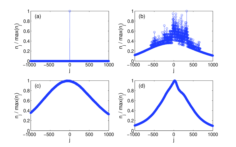
Figure 1: Pretreatment of massive data from rat EEG. Different types of distributions for Rat004 channel 02. For each panel, the $y$-axis is normalized by the maximum of $n_{j}$. The four panels correspond to: (a) a corrupted file with a large number of zeros (file $\#$20), (b) a bad recording with repetitions of oscillating patterns (file $\#$73), (c) a normal files without transitions (file $\#$77), and (d) a file containing a seizure (file $\#$99).

Figure 1 shows four typical types of $n_{j}$ distributions obtained from channel $02$ of Rat004 composed of $229$ data files. For binary files that have large numbers of continuous zeros, for example, file number $20$, the distribution is shown in Fig. 1(a). An example of a corrupted file is where a specific pattern of oscillations is embedded repeatedly in most of the data in the file. The corresponding distribution is shown in Fig. 1(b). The distributions from normal data files qualified for dynamical analysis are shown in Figs. 1(c) and 1(d). The distribution in Fig. 1(c) is approximately Gaussian. However, seizure events can cause distortions from the Gaussian distribution, as evidenced by Fig. 1(d) for file number $99$ where a clinically certified seizure is present. We observe that the distribution becomes somewhat narrowed (as compared with the case of no seizure) and slightly asymmetrical.

After obtaining the distribution for each file, we define and compute a statistical quantity for each file, and assemble the files within the same channel according to this quantity, as follows. Let $s_{k}=n_{k-N}-n_{k-N-1}$ ($k=1,\dots,2N$), where $s_{k}$ represents the difference between two neighboring counts, and let $\sigma_{s}^{2}=1/(2N-1)\sum_{k=1}^{2N}(s_{k}-\bar{s})^{2}$ be the variance, where $\bar{s}$ is the mean value of $s_{k}$. Note that $n_{j}$ is not normalized and their sum is the data length $L$ of the file. Denoting $\langle n\rangle_{j}$ as the smoothed curve of $n_{j}$, we have $\langle n\rangle_{j}\sim L$. The fluctuations, as characterized by $s_{k}$, are in general proportional to $\langle n\rangle_{j}$. As a result, the variance $\sigma_{s}^{2}$ is positively correlated with $L$, e.g., a larger value of $L$ would result in a larger value of $\sigma_{s}^{2}$.

Thus for small files that are normal in all other aspects, we will have smaller $\sigma_{s}$ values, which can be clearly identified from Fig. 2 as the points below the majority. This figure also shows some points with extremely large $\sigma_{s}$ values. These points correspond to the binary files with large numbers of continuous zeros [Fig. 1(a)]. The corrupted data all have $\sigma_{s}$ values in the range $10^{4}\sim 10^{5}$ [Fig. 1(b)], which can be excluded readily, as shown in the inset of Fig. 2. A transition in $\sigma_{s}$ at file number 99 (when the first seizure occurred) is observed.

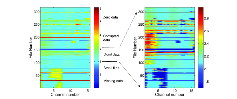
Figure 3: Contour representation of massive data from rat EEG. Contour plot of $\log_{10}\sigma_{s}$ for Rat001. Left panel shows the whole $\sigma_{s}$ range. Different types of data are classified according to the value of $\log_{10}\sigma_{s}$. In the right panel, the contour is for values of $10^{2}\leq\sigma_{s}\leq 10^{3}$ (good data), and the remaining values of $\sigma_{s}$ are set to $50$ so that the dark blue area marks all abnormal data.

By applying the same procedure to multiple channels, the massive EEG data from one rat can be expressed using a single contour plot of $\sigma_{s}$, as shown in Fig. 3. We can immediately identify different types of data in terms of the values of $\log_{10}\sigma_{s}$. It should be noted that for different “abnormal” situations, e.g., small files, contamination with zeros, or corrupted data, there can be different methods of remedy based on examining different aspects particular to the data. However, our method is general and efficient in that a single indicator is effective at distinguishing the different types of abnormalities in the files during the pre-processing stage of the massive database for further dynamical and statistical analysis.

II.2 EMD analysis of EEG data

We conducted extensive tests of applying the EMD procedure to EEG data (see Methods). A general finding is that the resulting IMFs in different frequency ranges possess statistical features that are relevant to certain brain activities, demonstrating that the EMD methodology can be effective for probing the dynamical origins of epileptogenesis. For example, typically the frequencies of the first 5 IMFs are about 5 kHz, 2 kHz, 1 kHz, 500 Hz, 200 Hz, 100Hz. Since the sampling frequency is 12 kHz, the first three modes correspond to mostly noise contained in the original EEG data. The fourth to sixth modes, whose frequencies lie in the range between 50 Hz and 800 Hz represent the intrinsic dynamical evolution of the underlying brain system.

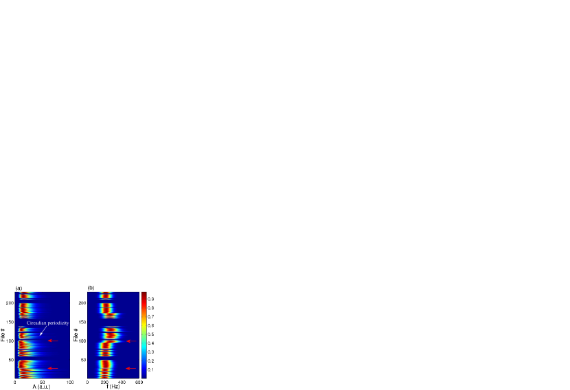
Figure 4: Typical EMD representation of massive rate EEF data. (a) Contour plot of normalized distribution of amplitude $A$ (in arbitrary units) varying in time of a particular EMD mode of interest (IMF5, around 200 Hz) for channel 11 in CA1 of EEG recording of a rat over a 2-month period. The all-blue region indicates corrupted files. Each file is a 7 hours recording at the sampling frequency $12$ kHz. Thus the vertical axis “File #” indicates time. The distribution is calculated and then normalized by the maximum value for each file. The rat underwent surgery between file 28 and file 29, and the first seizure occurred in file 99, as indicated by the red arrows. The comb-like structure indicates the circadian periodicity. (b) Normalized distribution of the frequency $f$ of the mode.

Our procedure for analyzing long EEG data thus consists of performing the EMDs to obtain different IMFs, calculating the amplitudes and frequencies of the IMFs that are deemed to reveal the dynamical evolution of the brain, and performing statistical analysis of the on-intervals for the IMFs in a proper frequency range. An example is shown in Fig. 4, where the distributions of the amplitude and frequency of an IMF for a particular channel of two-months’ duration are shown. The entire data set was divided into 230 files, each containing 7 hours of EEG recording. Note that when performing the EMD, the data is broken into small segments, e.g., 5 second for each segment, to make the computation more efficient. To calculate the IMFs, a 0.5 second segment is included at each end of the 5-second segment to eliminate the edge effect so that the IMFs can be accurately determined. From Fig. 4, we can distinguish the changes in the rat brain activity, such as stimulation and the occurrence of the first seizure. Recurrent seizures are not so clearly visible in this plot. Another apparent feature revealed is the circadian periodicity. The EEG recording has a 24 hour periodicity because of the circadian activity or of the external treatment of the rat such as feeding, etc., which also changes the frequency and amplitude of each decomposed IMF. Since each file is 7 hours long, the circadian periodicity indicates a periodicity of 3 (or 4) files in the plot, which is apparent from the comb-like structure in the plot, especially in Fig. 4(a), where adjacent two comb teeth have a separation of about 3 files.

II.3 Detection of HFOs and population spikes

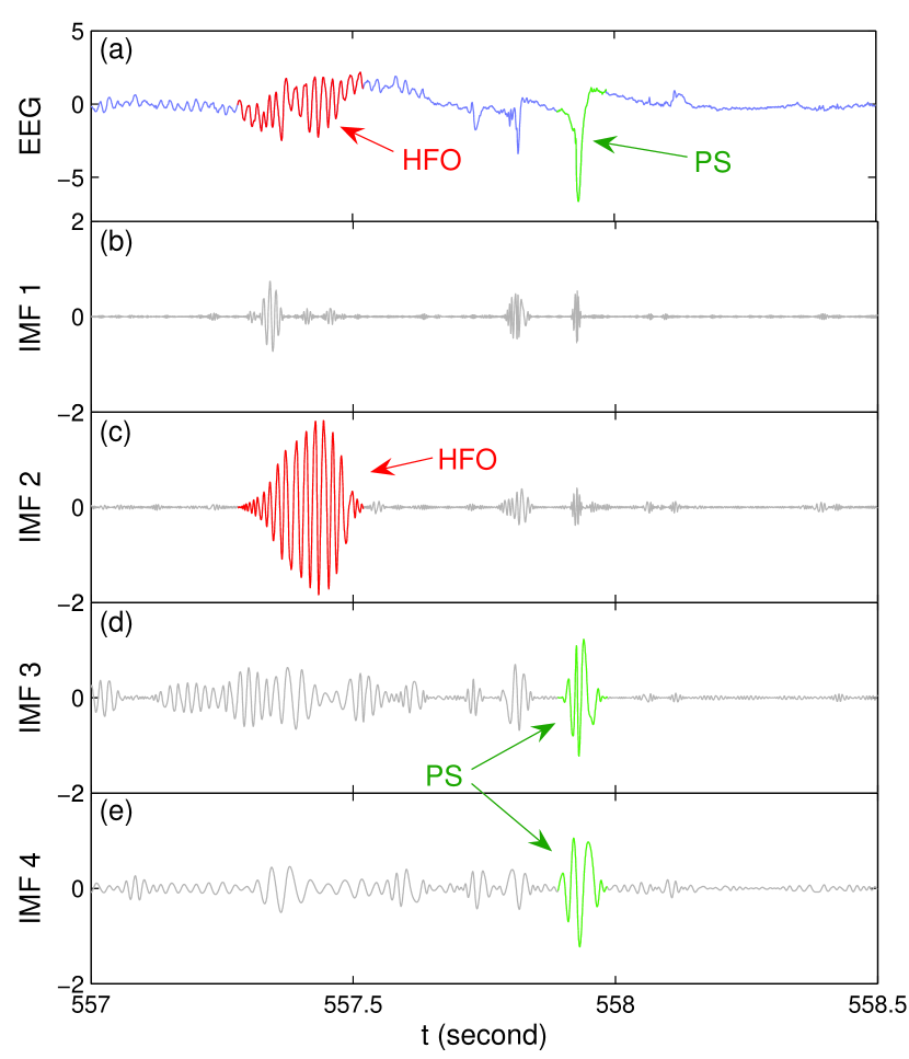
Figure 5: Example of EMD-based HFO detection from EEG data. A $1.5$ second segment of normalized EEG data containing an HFO and a population spike. (b)-(e) are the IMFs in the frequency range of interest. The HFO is revealed in IMF 2 and the population spike is revealed in IMF 3 and IMF 4.

To illustrate the detection of HFOs and population spikes, we reduce the sampling rate so that these dynamical events can be visualized clearly. Note that, when the sampling rate is reduced, the noisy components are effectively filtered out, so the first few IMFs become important. (In the detection of HFOs and population spikes, higher sampling frequency should still be used, in which case the first few IMFs need to be disregarded, as discussed above.) Figure 5 shows, for a segment of down-sampled EEG data, the relevant empirical modes. For this data set, the frequencies are 200-500 Hz for mode 1, 80-200 Hz for mode 2, about 50 Hz for mode 3 and 30 Hz for mode 4. Take mode 2 as an example, the IMF will have small amplitude if the original EEG data does not contain oscillations in the corresponding frequency range. When the EEG data contains these oscillations, they will be revealed in the corresponding IMF. Since HFOs are generally associated with frequencies larger than 80 Hz, they will be revealed in the first two modes. The population spikes (with a time scale of 0.1 s) are decomposed by EMD into oscillations in the frequency range 10-50 Hz, thus they will mainly be manifested in modes 3 and 4. The EEG data in Fig. 5(a) contains an HFO and a population spike. It is apparent that the HFO and population spike are separated by EMD into different modes and are localized in different time scales, e.g., Fig. 5(c) for the HFO and Figs. 5(d,e) for the population spike. Thus the amplitude of the modes evolving in time can be used to detect the HFOs or population spikes, depending on the frequency range of the mode.

Our results thus suggest strongly the feasibility of developing EMD based algorithms to systematically detect all the HFOs and population spikes. In this regard, we note an existing method of detection of HFOs, which employs short-time energy or line length of the acquired data for HFOs in some small frequency ranges GWMDL:2007 . Our method is capable of detecting HFO and can be used to distinguish various oscillation profiles. Based on the detected HFOs and population spikes, extensive statistical analyses for the five critical phases during epileptogenesis, namely, pre-stimulation state, pre-seizure state, status epilepticus phase, epilepsy latent period, spontaneous/recurrent seizure period, can be carried out to gain unprecedented insights into epileptogenesis.

It can occur that, for a particular signal whose highest frequency component is most significant to the underling dynamics, the first IMF contains the dominant dynamics with the highest frequency, the next is a lower frequency background to it, and so on. However, while the first IMF is the highest frequency component, the corresponding frequency range may not necessarily be relevant to the system dynamics. In fact, we found that typically the first IMF corresponds to noise, and the next IMF contains information about the dynamics of the system. Which IMFs are actually useful and informative depends on the nature of the original signal. More specifically, what EMD does is to decompose the signal into different frequency components through different IMFs, which contain the time varying amplitude and frequency information for each component embedded in the original signal. If the signal is contaminated by noise, the first IMF would be the noise component that contains little information about the underlying dynamics. Our analysis of the massive EEG data indicates that this is indeed the case.

II.4 Automated detection and classification of HFOs

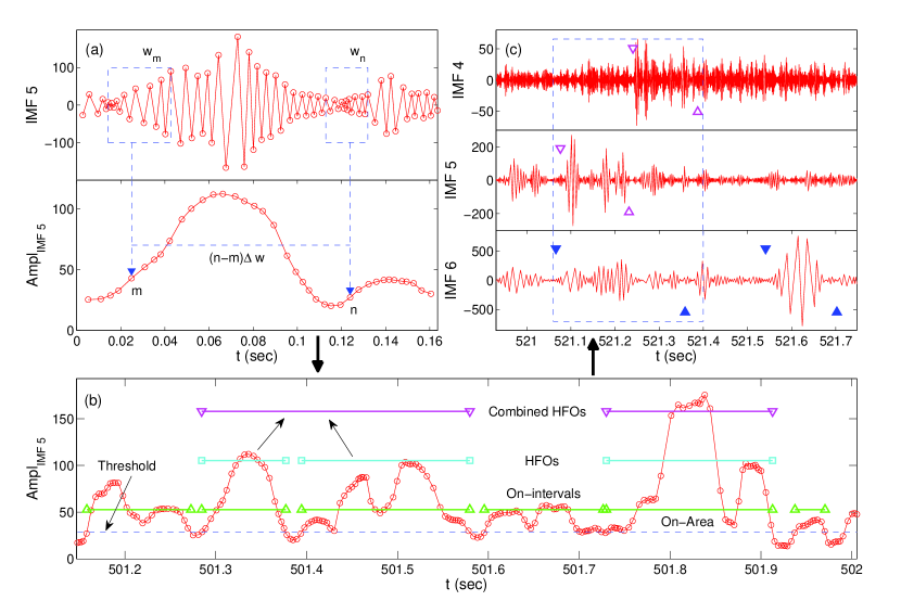
Figure 6: Illustration of HFO detection method. The method consists of three steps. (a) Computing the amplitude function from each IMF generated by EMD. The size of the moving window is $w=7$ periods (indicated by the blue dashed boxes). The time step for the moving window is $\Delta w$. (b) For each IMF, we locate the on-intervals, find HFOs, and combine adjacent HFOs if they are too close to each other. The blue dashed line is the threshold chosen for the segment of the amplitude function. (c) Classifying HFOs in terms of their frequencies, e.g., ripples (solid blue triangles), fast-ripples (open magenta triangles), and then combining overlapping HFOs across different IMFs, as shown in the blue dashed box.

Our method to detect, characterize, and understand HFOs from EEG recordings consist of the following steps: (1) performing EMD and calculating distinct IMFs, (2) searching for HFOs based on the amplitudes of IMFs, and (3) classifying HFOs in terms of their frequencies and calculating the statistical properties of HFOs. An illustration of the steps is shown in Fig. 6.

We first calculate the amplitudes of the IMFs from an automated EMD procedure. We then locate the extrema of one IMF and define the interval between two neighboring maxima (or minima) to be one period $T$, as shown in Fig. 6(a). Unlike the Fourier transform that becomes ineffective in time-series analysis when the signal frequency changes with time, EMD is well suited for generating IMFs whose frequencies vary with time, i.e., when the period is a function of time: $T=T(t)$. We set a moving time window of size $w$ and calculate the average IMF amplitude within the window. The window contains a fixed number of IMF periods. Since the period varies with time, the actual time span of the window also changes with time. As an example, we show in Fig. 6(a) two windows $w_{m}$ and $w_{n}$, each containing the same number (7) of IMF periods. Apparently, their sizes are different. The amplitude values are weighted magnitudes and are calculated as $A_{m}=(1/2)\sum_{i\in w_{m}}(x_{i+1}-x_{i})(|y_{i+1}|+|y_{i}|)$, where $x_{i}$ and $y_{i}$ are the position and magnitude of the IMF, respectively, and the factor $(x_{i+1}-x_{i})$ is the corresponding weight. The calculation is repeated when the window is moved to the next position by the step size $\Delta w$, which is also chosen to contain a certain number of IMF periods. Small values of $w$ and $\Delta w$ result in rapidly oscillating amplitude functions, whereas too large values of $w$ and $\Delta w$ would cause a loss of information. Empirically, the window size can be chosen to include several IMF periods, e.g., six to nine, where the moving forward step size $\Delta w$ can be set as one.

The next step is to find on-intervals, time intervals when the amplitude values are larger than a certain threshold $A_{c}$, as shown in Fig. 6(b). To set a proper threshold, we can pick a segment (e.g., one hour long) from the amplitude data and calculate the mean $\mu$ as well as the standard deviation $\sigma$. One way to set the threshold is $A_{c}=a_{\mu}\mu+a_{\sigma}\sigma$, where $a_{\mu}$ and $a_{\sigma}$ are two adjustable parameters on the order unity. To characterize each on-interval $O_{i}$, we define an on-area $S_{i}$, the area of the IMF in the on-interval above the threshold:

$$S_{i}=(1/2)\sum_{j\in O_{i}}(x_{j+1}-x_{j})(A_{j+1}+A_{j}-2A_{c}),$$ (1)

where $x_{j}$ and $A_{j}$ are the position and magnitude of the amplitude function of the underlying IMF, respectively. The notation $S_{i}$ with the capital $S$ should be distinguished from $s_{k}$ that denotes the difference between two neighboring counts. On-intervals are sorted in the descending order in terms of their on-areas: $S_{1}>S_{2}>\cdots$. The HFOs are identified as those with the largest on-areas, i.e., with longer duration and larger oscillating amplitudes. Since the on-area values of HFOs are typically much larger than those of non-HFO on-intervals, the HFOs can be reliably identified as the outliers in the on-area statistics, as follows.

Starting from the most significant on-interval $O_{1}$, we can evaluate its on-area $S_{1}$ with a score function of the remaining on-intervals. If

$$S_{1}>\alpha E[\{S_{i}\}_{i\geq 2}]+\beta\sqrt{\mathrm{Var}[\{S_{i}\}_{i\geq 2}]},$$ (2)

$O_{1}$ will be identified as an HFO, where $\alpha$ and $\beta$ are two adjustable parameters, and $E[\cdot]$ and $\mathrm{Var}[\cdot]$ are the expectation and variance functions. This process is repeated until no on-intervals in the remaining sequence satisfy the criterion. Typically, for one IMF, approximately $10\%$ of the on-intervals would be selected as HFOs. Among the remaining HFOs, one can see that some are so close to each other that it is reasonable to combine them. The combinations are carried out wherever the gap $G$ between two neighboring HFOs is small, i.e., when $G<g\cdot\min(T_{HFO_{1}},T_{HFO_{2}})$, where $g$ is the parametric gap tolerance ratio and $T_{HFO}$ is the HFO duration. An example of combining HFOs is shown in Fig. 6(b).

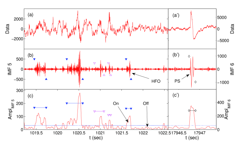
Figure 7: Example of successful HFO and PS detection. (a) Original EEG data plot of about 3 seconds. (b) IMF 5 plot with solid blue triangles marking the ripples and open magenta triangles marking the fast-ripples. (c) The amplitude of IMF 5. The horizontal blue line is the threshold for separating on/off intervals of HFOs. The threshold is calculated from the amplitude data segment of about one hour. The computational parameters are $a_{\mu}=1$ and $a_{\sigma}=1$. (a’)-(c’) The original data, IMF6, and its amplitude function, respectively. The black diamonds mark the position of the population spikes.

HFOs in different frequency ranges are usually responsible for different brain behaviors such as normal information processing and spontaneous seizures. The third step of our procedure is to calculate the frequencies of various HFOs, which is done by locating the starting and ending times of an HFO, finding the number $n$ of oscillating periods within it, and dividing by its duration: $f=n/T_{HFO}$. When necessary, we combine overlapping/nearby HFOs, as shown in Fig. 6(c). When various HFOs have been identified, we can classify them into distinct frequency ranges: low-frequency range ($<80$Hz), ripples [$80\sim 200$Hz, between pairs of solid blue triangles in Fig. 6(c)], and fast-ripples [$>200$ Hz, between pairs of open magenta triangles in Fig. 6(c)]. HFOs of frequencies lower than $80$Hz are identified as population spikes. An example of identifying and classifying HFOs is shown in Fig. 7.

II.5 Statistical and scaling properties of HFOs

As described, the on- and off-intervals associated with HFOs can be determined by setting a threshold value $A_{c}$ in the amplitude function of a given IMF. For a given HFO, an on-area can then be defined, which is the area of the portion of the amplitude function above the threshold. The most significant HFOs are those with the largest on-areas. The on-intervals thus provide a base for characterizing the HFOs. Intuitively, HFOs of various magnitude correspond to “islands” of various sizes above the “sea” level defined by the threshold. To obtain a more complete understanding of HFOs, it is insightful to examine the corresponding “undersea” dynamics (below the threshold). It is computationally feasible to study the dynamical and statistical characteristics of the oscillations below the “sea” level but only within a certain depth.

To illustrate our approach in a concrete way, we take the example in Fig. 7 and focus on mode 5 because the frequency of this mode lies in a suitable HFO frequency range. From the contour plot of the distribution of amplitude versus file number, Fig. 4, we see that there are several regions of distinct properties. In particular, the EEG data are relatively stable before the stimulation, say between files 28 and 29. After the stimulation, the data changed characteristically, as can be seen from the amplitude distribution plot in Fig. 4(a) (indicated by the arrow between files 28 and 29). The first seizure occurred in file 99, and the data are stable for files 29-99. There is a relatively small change between files 51 and 52, as can be seen from the amplitude plot in Fig. 4(a), when the rat was actually moved from one cage to another. We have checked other modes and also data from other channels and found a consistency in the specific data segmentation as described. It is thus useful to study these different segments separately: files 1-28 (before stimulation), files 29-51 (between stimulation and first seizure), files 52-94 (preictal phase), files 100-172 (postictal phase but with recurrent seizures in files 105 and 125), and files 175-223 (with recurrent seizures in files 192, 209, and 216). To obtain stable statistics, we temporally disregard a few files that are in the transitional regime. However, these files may be important in providing possible hints about how the seizure (e.g., the one occurred around file 99) is developed in terms of the transient dynamics. The specific segmentation scheme of the EEG data is only for one rat, but it is valid for all the channels.

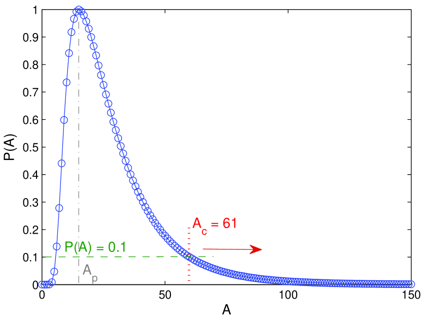
Figure 8: Determination of threshold $A_{c}$. Normalized distribution $P(A)$ of the amplitude $A$ for files 1-28 for the same mode as in Fig. 4, where $A_{p}$ is the value of amplitude at the peak of the distribution. For example, by setting $P(A)=0.1$ and assuming that $A_{c}>A_{p}$, $A_{c}$ can be determined to be 61. If $P(A)$ takes a smaller value, then $A_{c}$ will be larger.

For different segments the signal amplitudes can have systematic differences, and in certain cases the average amplitude can be, for example, twice larger in one segment than in another. It is thus necessary to determine and set different thresholds in different segments. To do this, first we calculate the normalized distribution of the amplitude $A$ in each segment. The distribution for files 1-28 is shown in Fig. 8. Second, from the peak point defined as $P(A_{p})=1$ (since $P$ is normalized to unity), we decrease $P$ with small steps, e.g., $P=0.98,0.96,...,0.02$. For for each $p$ value, we determine the corresponding threshold $A_{c}$ ($>A_{p}$), as demonstrated in Fig. 8 for $P=0.1$, where the corresponding threshold is $A_{c}=61$. Third, for each value of $A_{c}$, we calculate all the on-intervals in this segment from the amplitude function. The distributions of the durations $T$ of the on-intervals from different segments are then compared, and various threshold values are set such that the values of $P(A_{c})$ are all identical across the segments.

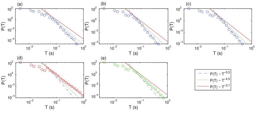
Figure 9: Statistical and scaling behaviors of HFOs. Distributions of on-interval $T$ of IMF 5 (channel 11, Fig. 4): (a-e) for files 1-28, 29-51, 52-94, 100-172, 175-223 respectively. The numbers of on-intervals are 344310, 314698, 431674, 498947, and 510096 for (a-e), respectively. An algebraic distribution is observed with different exponents for different segments. The exponent for the solid, dotted, and dash-dotted lines are -3.7, -4.5, and -5.5, respectively. The threshold $A_{c}$ is chosen such that $P(A_{c})=0.02$ for all the segments.

Figure 9 shows an example of the statistical distribution of the on-intervals for all five segments as specified above. We observe algebraic distributions. For each segment, the algebraic scaling regime extends over at least one order of magnitude in the length of the on-interval. The distributions for the three segments before the first seizure have approximately the same algebraic scaling exponent, as shown in Figs. 9(a-c), although the amplitude value varies continuously for these segments, as shown in Fig. 4. After the first seizure, the exponent becomes smaller, indicating more on-intervals with longer durations. For example, in Fig. 9(d), for on-intervals with $T\sim 0.4$ s, the probability is 100 times larger than those before the seizure. For files 175-223, however, the exponent is somewhat increased, signifying a decrease in the probability of longer on-intervals, but it is still larger than the probability before the seizure. We have systematically checked on-interval statistics for different thresholds. The algebraic scaling and the qualitative difference among the scaling exponents from different segments are robust with respect to variations of the threshold in a certain range (e.g., $P(A_{c})$ ranging from 0.02 to 0.3).

Since many on-intervals (especially the long ones) correspond actually to HFOs, our discovery of the algebraic scaling suggests that the HFOs appear more active and sustaining associated with seizure activities, which is consistent with previous observations WGSH:2008 ; BES:2010 ; CNHC:2010 . In general, an algebraic scaling indicates a hierarchical organization in the underlying dynamics, which in our case, suggests such an organization in the brain neuronal activities. For example, the local synchrony among discrete neuron clusters may vary in hierarchical scales. The fact that approximately the same algebraic scaling exponent occurred before the seizure indicates that, after the stimulation, while evolving toward epilepsy, the underlying dynamics behave the same as in the normal brain. This could be due to the latency effect of the stimulation. The development into epilepsy, however, occurs in a relatively short period due to the cascading effect similar to that associated with earthquakes OFSML:2010 .

We have also checked other channels, which are so selected that they belong to different (neural) correlation clusters. For some channels, behaviors similar to those in Fig. 9 are observed, but significant deviations occur for some other channels. This may be due to that the HFO and the seizure onset zone are usually highly localized CNHC:2010 . As a result, only within a proper range of this zone can the HFOs be detected. Since the distance between the neighboring channels is quite small (about $0.25$ mm), the HFO and the underlying neuronal activity could be revealed only in a small subset of channels.

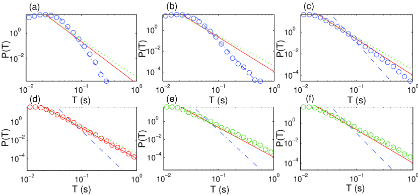
Figure 10: Statistical and scaling behaviors of HFOs - more examples. Distributions of on-interval $T$ of IMF 5 (channel 6 of rat 9): (a-f) for files 1-19, 32-57, 63-72, 78-97, 98-118, and 119-149, corresponding to the pre-stimulation state, post-stimulation state, evolving towards seizure, status epilepticus phase, epilepsy latent period, and spontaneous/recurrent seizure period, respectively. The numbers of on-intervals are 354499, 561669, 300291, 458649, 293118, and 438919 for (a-f), respectively. An algebraic distribution is observed with different exponents for different segments, where the exponents are $-5.7$, $-3.3$, $-2.9$ for dash-dotted line, solid line, and dotted line, respectively. The criterion for choosing the threshold $A_{c}$ is the same as in Fig. 9

We find that the algebraic scaling law for the on intervals of HFOs holds for all the animal models. Figures 10(a-f) show more examples for a different rat. In particular, the scaling was calculated for a specific channel for the pre-stimulation state, post-stimulation state, evolution towards seizure, the status epilepticus phase, the epilepsy latent period, and the spontaneous/recurrent seizure period, for panels (a-f), respectively. We see that, while the details of the scaling behaviors can be different for the distinct critical phases (e.g., during epileptogenesis the on-intervals with longer durations are dominant after the first seizure), the algebraic nature of the scaling law is robust.

III Discussion

Seizure prediction, early recognition, and blockage of seizures are considered by the membership of the American Epilepsy Society (AES) as the first research priority listed among fifteen. To achieve these goals a good understanding of the origin, mechanism, and dynamics of seizures is necessary. At present the only accessible avenue to probe the origin of epileptic seizures is multiple-channel EEG or ECoG data. Continuous improvement in the experimental methodology has made such data highly reliable and generally of high quality. A challenge is that the amount of EEG or ECoG data is massive. An issue of paramount importance and significant interest is to extract knowledge about epilepsy from data.

We have developed a method to detect, characterize, and analyze the dynamical behavior of HFOs from a massive database of extensive EEG recordings of a number epileptic rats over two months. We first devise a general and efficient procedure for pre-processing the massive database to exclude erroneous data segments and statistical anomalies. (The procedure should also be applicable to massive data sets of other sorts, such as large-scale sensor data or seismic data collections.) We then articulate a procedure based on separating the time scales, the EMD method Huangetal:1998 ; YL:1997 , to detect HFOs. Due to its built-in ability to pick out from a complex, seemingly random time series a number of dominant components of distinct time scales, the method has proven to be especially effective for the detection of HFOs. We finally perform a statistical analysis and find evidence for a striking phenomenon: the occurrences of HFOs appear in an on-off intermittent manner and the time intervals that they last exhibit an algebraic scaling.

The methods and results in this paper can potentially be extended to other fields. For example, a previous work OFSML:2010 indicated that seizures can be regarded as “quakes of the brain.” It is then conceivable that the idea, method, and algorithms developed here can be extended to big seismic database for detecting anomalous oscillating signals (similar to HFOs) preceding the actual occurrence of earthquakes.

Big data sets arise not only in biomedicine, but also in other fields of science and engineering. For example, in civil engineering, large sensor arrays are often employed to monitor the temperature, humidity, and energy flows in large, complex infrastructure systems in a continuous-time fashion. In such an application the underlying system is in general nonstationary and nonlinear, and to detect behaviors that deviate from the norm or the expected is of considerable interest. Another example is earthquake data. A previous work OFSML:2010 indicated that seizures can be regarded as “quakes of the brain.” It is then conceivable that the idea, method, and algorithms developed in this paper can be extended to big seismic database for detecting anomalous oscillating signals (similar to HFOs) preceding the actual occurrence of earthquakes. In general, the EMD/Hilbert transform based methodology demonstrated in this paper has broad applications because it is specifically designed Huangetal:1998 to deal with nonlinear and nonstationary systems. Due to its built-in ability to obtain from a complex, seemingly random time series a number of dominant components of distinct time scales, the method is anticipated to be especially effective for anomaly detection. A challenge is to develop mathematically justified, computationally reasonable and automated procedures to detect anomalies, from big data sets, which has been addressed in this paper through the detection of HFOs from massive EEG data with multiple animal models.

We now discuss a number of issues that may warrant future efforts.

First, there is room to improve the EMD-based algorithms developed in this paper, leading possibly to a fully automated method for detecting HFOs and population spikes from massive data for all distinct epileptic stages including pre-stimulation, pre-seizure and recurrent seizures. This will provide a base for probing into the emergence and evolution of HFOs through detailed analyses using methods from nonlinear dynamics, statistics, and statistical physics. Special features associated with different types of brain activities can be identified, with the grand goal to exploit the predictive power of HFOs for epileptic seizures. Many questions, which are previously unimaginable, can be asked. For example, does a general class of HFOs exist, regardless of the specific brain activities? What types of HFOs are especially related to seizures? How localized are they around the regions of seizure onset? Are there systematic and characteristic changes in the HFOs during the ictal phase? What types of HFOs are associated with recurrent seizures and is there any relation to the latency period? Answers to those questions and many more will provide a comprehensive picture for the dynamical role of HFOs in epileptogenesis.

Second, with our optimized EMD-based method, HFOs and population spikes can be detected reliably for all the channels. The issue of spatiotemporal evolution of these dynamical events in the brain can then be addressed. For example, we have observed that certain population spikes appear only in some channels at a given time, i.e., they may be highly localized in space. Some HFOs can, however, occur in many channels simultaneously. A possible reason for the dispersive character of the HFOs is that the distance between neighboring recording sites is about 0.25mm, which can be within the propagating range of the underlying neuronal activities that cause the pathological HFOs. The available database from a dense electrode grid thus provides a useful probe to study the propagation of neuronal synchronous activities. For example, by examining the exact timings of HFOs and population spikes and the occurrence of the epileptic seizure in different EEG channels, the propagating pattern of these dynamical events can be determined and, consequently, the sources triggering these events may be identified. A mapping between the epileptic dynamics and activities in different brain regions can be made and the temporal evolution of the mapping can be studied. It would also be useful to examine the correlation patterns of the distinct dynamical events and compare them with those of the background neuronal activities. All these have the potential to provide deeper insights into the origin of epileptogenesis.

Third, in this paper we focused on stable states of the brain, which are the states that last for relatively long periods of time. The transient behaviors were neglected. It would be interesting to study the nonlinear and complex transient dynamics LT:book associated with epileptogenesis and brain behaviors in general.

Fourth, there were previous studies of exploiting nonlinear dynamics for analyzing epileptic seizures (e.g., Refs. OHLF:2001 ; LOHF:2002 ; LHFO:2003 ; LHFO:2004 ; HOFAL:2005 ; LFO:2006 ; LFOH:2007 ), and on-off intermittency is an ubiquitous phenomenon in nonlinear dynamical systems FY:1985 ; FY:1986 ; FIIY:1986 ; PST:1993 ; HPH:1994 ; PHH:1994 ; HPHHL:1994 ; SO:1994 ; LG:1995 ; VAOS:1995 ; AS:1996 ; Lai:1996a ; Lai:1996b ; VAOS:1996 ; MALK:2001 ; RC:2007 . It is known in nonlinear dynamics that on-off intermittency can be controlled by applying small but deliberately chosen perturbations to the system NHL:1996 . The power-law statistics of the on-intervals associated with HFOs indicate the emergence of a hierarchical organization in the neuronal activities. However, it is difficult to determine uniquely the underlying dynamical mechanism that is distinct from the well documented mechanism for on-off intermittency. Nonetheless, there are common features between the intermittent behaviors of HFOs uncovered in this paper and those of on-off intermittency, such as scaling properties. If a specific type of HFO can be correlated with the occurrence of seizures and if the underlying dynamics bear similarity to those of generic on-off intermittency, it may be possible to investigate controlling HFO dynamics based on previous works on controlling on-off intermittency. In particular, can the on-off intermittent dynamics of the epileptic HFOs be controlled by using, say, small and infrequent brain stimuli to delay or even eliminate seizures? The results in this paper provide a base for developing computational and experimental schemes to test this control idea.

IV Methods

All experiments on live vertebrates (rats) were performed in accordance with the guidelines and regulations of National Institute of Health and University of Florida. All experimental protocols were approved by University of Florida.

IV.1 Setting of experimental data collection

Experiments were performed on five, two-month old, male Sprague Dawley rats, each weighing between 210 and 265 g. The rats were induced into the state of complete anesthesia by subcutaneous injection of 10 mg/kg (0.1 mL by volume) of xylazine and maintained in the anesthetized state using isoflorane (1.5) administered through inhalation by a precision vaporizer. For each rat, the top of its head was shaved and chemically sterilized with iodine and alcohol. The skull was exposed by a mid-sagittal incision. In three of the five rats, a bipolar, twisted, Teflon-coated, stainless steel electrode (330$\mu$m) was implanted in the right posterior ventral hippocampus (5.3mm caudal to bregma, 4.9 mm right of midline suture and at a depth of 5 mm from the dura) for stimulating the rat into status epilepticus. The remaining two rats are for control. In all the five rats a 16 microwire (50 $\mu$m, TDT Technologies, Alachua, FL) electrode array comprising of two rows separated by 500 $\mu$m with electrode spacing of 250 $\mu$m, was implanted to the left of midline suture horizontally in the CA1-CA2 and dentate gyrus of the hippocampus. The furthest left microwire was 4.4 mm caudal to bregma, 4.6 mm left of midline suture and at a depth of 3.1 mm from the dura. A second microwire array of 16 electrodes was implanted to the right of midline suture in a diagonal fashion. The furthest right microwire was 3.2 mm caudal to bregma, 2.2 mm to the right of midline suture. The closest right microwire was 5.2 mm caudal to bregma, 1.7 mm to the right of midline suture and at a depth of 3.1 mm from the dura. Finally four 0.8 mm stainless steel screws were placed in the skull to anchor the microwire electrode array: two screws were AP 2 mm to the bregma and bilaterally 2 mm and served as the ground electrodes while two screws were AP -2 mm to the lambdoidal suture and bilaterally 2 mm and served as the reference electrodes. The entire surgical area was then closed and secured with cranioplast cement. Following surgery the rats were allowed to recover for a week.

IV.2 Data acquisition and file structures

Electrophysiological recordings were conducted by hooking each rat onto a 32-channel commutator, the output of which was fed into the recording system comprised of two 16-channel pre-amps, which digitized the incoming signal with a 16 bit A/D converter at a sampling rate of 12kHz ($\sim 12207$ Hz). The digitized signal was then sent over a fiber optic cable to a Pentusa RX-5 data acquisition board (Tucker Davis Technologies), where the signals were bandpass-filtered between 1.5 Hz and 7.5 kHz. The digital stream of data was stored for later processing. For each channel, the data were recorded and saved as $16$-bit signed integer binary files, each of size $600-700$ megabytes ($\sim 7.5$ hours recording time). Thus, for each rat, there were $32$ channels, each of which has between 153 and 317 files depending on the recording durations. Each binary file was assigned a rat number, a channel number, and a file number. The data were recorded over 2 months for most of the rats, including pre-stimulation stage, pre-seizure stage, status epilepticus phase, epilepsy latent period, and spontaneous/recurrent seizure period.

The sampling rate of the data was relatively high, making it possible to analyze high frequency, short duration dynamical events in the brain such as HFOs and population spikes. The typical duration of an HFO is about 100 ms and its characteristic spontaneous frequency can be as high as several hundred Hertz. In such a case, our data will have 40 points for a single oscillation period, which is generally enough for various analyses of HFOs. The extensive database provides us with a platform to compare the high frequency events in different stages in the evolution of epileptic seizures and to systematically investigate the dynamics of epileptogenesis.

IV.3 Empirical Mode Decomposition (EMD) of EEG data

EMD is specifically designed to deal with nonlinear and non-stationary data sets. In particular, EMD decomposes the signal into a series of intrinsic mode functions (IMFs), as follows. For a given signal, EMD determines the local maxima and local minima, and connect them with cubic splines to form an IMF. One then subtracts the IMF from the original signal, and repeats the process to get the second IMF, and so on. The procedure is repeated until the remaining signal becomes monotonic. The IMFs are orthogonal to each other (at least locally) and their sum restores the original data. Thus, effectively, the original signal has been decomposed into the IMFs, each in a distinct frequency range, whose non-stationary amplitude and frequency information is well preserved.

Ideally, for a given EEG data, the EMD method returns a set of IMFs in separate frequency ranges. Practically, since each data file is too large to be processed computationally, we need to divide the data into small segments so that each segment can be computed within the memory of our computers. To deal with the boundary effect properly, for each data segment, we include an extra but much smaller subset of data points on both ends of the segment, which are from neighboring segments. These are the corresponding boundary sets. After performing the EMD calculations, only the IMFs within the original data segment are kept, while those associated with the boundary sets are discarded. For a given data segment, the resulting IMFs usually depend on the choices of the sizes of the segment and the boundary sets. In particular, the larger the boundary sets, the more accurate the IMFs, but the amount of the computation will also increase. A systematic test on varying sizes of the boundary sets indicates that the choice of 0.5-second duration (corresponding to 6103 data points at the recording sampling frequency) for each boundary set yields accurate IMFs with tolerable extra computation load. The limited computational power also stipulates that the size of each segment itself cannot be too large. Our systematic test gave 5 seconds (about 61035 data points) as the optimal duration for balancing the computation time and the reliability of the results. We use the code developed by Rilling et al. EMDcode to perform the EMD calculations by modifying the original C-Matlab interface to C-codes.

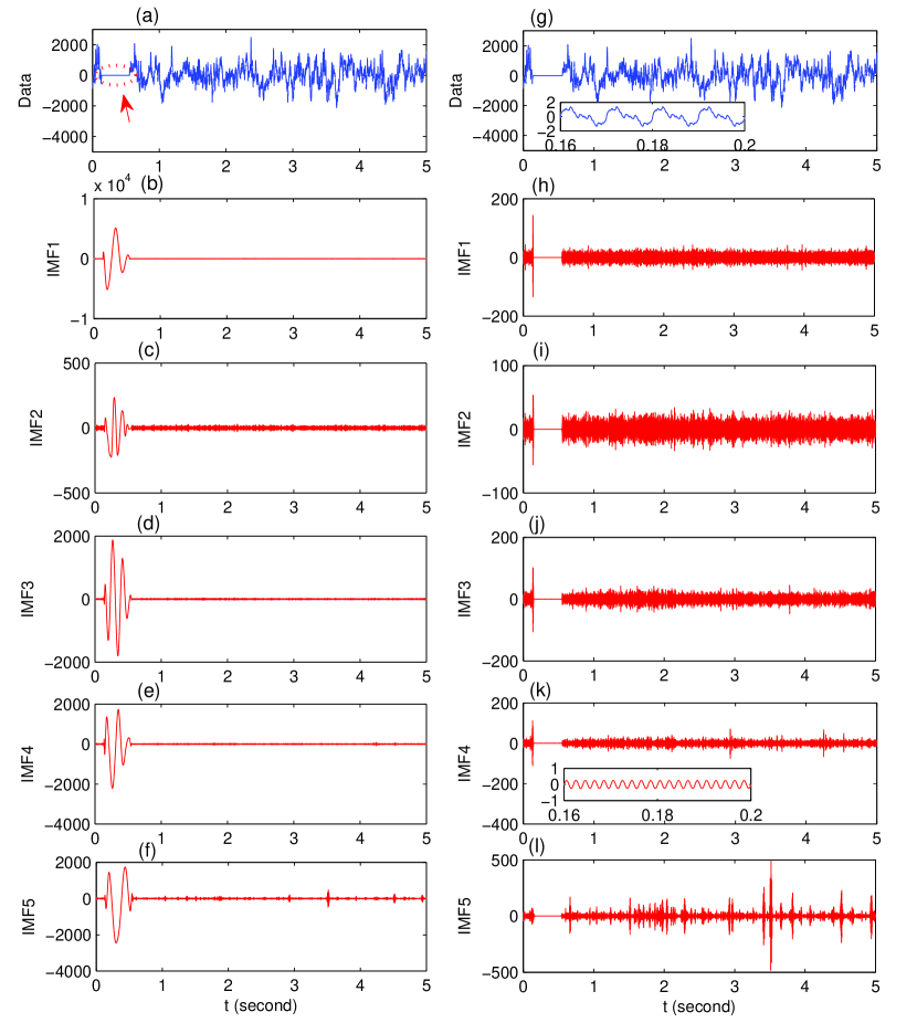
Figure 11: A demonstration of adding small oscillations in EMD computation to eliminate edge effect. (a) A 5 second segment of data with about 0.4 second zeros, as indicated by the dotted circle. (b-f) The first 5 intrinsic mode functions directly calculated from the data in (a). (g) Data (a) with added small oscillations on the scale of unity (see text), which is almost invisible from the figure. (h-l) The first 5 intrinsic mode functions calculated from the data in (g). Insets of (g) and (k) show magnification of the zero region. Note that the scale of the $y$ label is much larger in (b-f) than those in (h-l). The anomalies appeared in (b-f) are effectively removed by the simple method of adding small oscillations at the boundaries of the data segment.

Another practical issue is that the data may contain some discontinuities. In such a case, the EMD program may diverge or have abnormally large values [Fig. 11(a-f)]. A remedy is to add a small perturbation in the original signal prior to the EMD calculations. However, due to the difference in the frequency ranges in which the various IMFs lie, small time-varying perturbation signals of frequencies in these distinct ranges are needed. For each frequency range, the amplitude of the perturbation needs to be orders of magnitude smaller than that of the corresponding IMF. For example, if for a normal EEG data segment (denoted by $y[i]$), there are six IMFs and their frequencies are about 5 kHz, 2 kHz, 1 kHz, 500 Hz, 200 Hz, and 100 Hz, respectively (for IMFs 1-6), we will need to add the following small sinusoidal signals: $y[i]=y[i]+0.9\times\sin{(2\pi i/(12207/100))}+0.5\times\sin{(2\pi i/(12207/200))}+0.25\times\sin{(2\pi i/(12207/500))}+0.125\times\sin{(2\pi i/(12207/1000))}+0.0625\times\sin{(2\pi i/(12207/2000))}+0.03\times\sin{(2\pi i/(12207/5000))}$, where the amplitudes of the IMFs are typically larger than 10. The perturbation signals thus will not have any practical influences on the IMF results for normal data. However, when there is a discontinuity with a linear relaxation in time, the corresponding IMFs will contain the added small sinusoidal oscillations instead of generating divergence or large anomalies [Fig. 11(g-l)]. In addition, when the original data is contaminated by a small segment of zeros, without adding the small oscillations, the resulting IMFs will oscillate wildly in this region with amplitudes orders of magnitude larger than those of the normal data sets [Fig. 11(a-f)]. This is because, for obtaining each IMF, EMD looks for the local maxima and local minima and then approximate the data with cubic spline connecting the maxima or minima. When a segment of zeros is encountered, there are no local maxima or minima so that the EMD extrapolates with cubic spline using the maxima or minima outside this region. For the first IMF, since the frequency is the highest (about 5 kHz), even a zero segment of about 0.1 second would correspond to about 500 maxima or minima. Thus the extrapolation will generate extremely large, artificial oscillations. The remainder obtained by subtracting IMF 1 from the original data will compensate the large oscillations in IMF 1, but they will propagate to subsequent IMFs. The conclusion is that, adding the small sinusoidal perturbing signals causes essentially no difference in the original signal (about 1 part in 1000), but the artificial anomalies can be effectively eliminated.

Research Ethics

Human datasets were not used.

Animal ethics

Experiments were performed on 2-month old male Sprague Dawley rats. This study was conducted in accordance with Federal and University of Florida Institutional Animal Care and Use Committee policies regarding the ethical use of animals in research. (IACUC protocol D710).

Permission to carry out fieldwork

No fieldwork was performed

Data Availability

All data used in the study have been uploaded onto Google Drive and are publicly available. The link is https://drive.google.com/drive/folders/0B7S5nQOU_-nMIYkEyYmJvTGpNOVU?usp=sharing.

V Competing Interests

We have no competing interests.

Authors’ Contributions

YCL, LH, PRC, WLD and MLS conceived and designed the research. The data was acquired in PRC’s lab. LH and XN developed the computational method and performed simulations. All analyzed data. YCL and LH drafted the manuscript. All authors gave final approval for publication.

Funding

The National Institutes of Biomedical Imaging and Bioengineering (NIBIB) through Collaborative Research in Computational Neuroscience (CRCNS) Grant Numbers R01 EB004752 and EB007082, the Wilder Center of Excellence for Epilepsy Research, and the Children’s Miracle Network supported this research. This work was also supported by the US Army Research Office under Grant No. W911NF-14-1-0504. LH was supported by NNSF of China under Grants No. 11135001, No. 11375074, and No. 11422541. Y.C.L. would like to acknowledge support from the Vannevar Bush Faculty Fellowship program sponsored by the Basic Research Office of the Assistant Secretary of Defense for Research and Engineering and funded by the Office of Naval Research through Grant No. N00014-16-1-2828.

Figure 2: Statistical properties of massive data from rat EEG. Standard deviation $\sigma_{s}$ for Rat004 channel 02. Red circles denote the normal files; green squares are the files with large numbers of zeros; blue crosses are corrupted files; pink diamonds are small files; cyan triangles are small files with many zeros; black star is small corrupted files. The arrow marks the file $99$ which has the first seizure. The inset shows the enlarged area around file $99$ on a linear scale.

.

References

- (1) Marx V. 2013 Biology: the big challenges of big data. Nature (London) 498, 255–260.
- (2) Sagiroglu S, Sinanc D. 2013 Big data: a review. In 2013 International Conference on Collaboration Technologies and Systems (CTS), San Diego, CA, 42–47.
- (3) Katal A, Wazid M, Goudar RH. 2013 Big data: Issues, challenges, tools and good practices. In Sixth International Conference on Contemporary Computing (IC3), Noida, 404–409.
- (4) Chen M, Mao SW, Zhang Y, Leung VCM. 2014 Big Data Related Technologies, Challenges and Future Prospects. Berlin: Springer.
- (5) Fan JQ, Han F, Liu H. 2014 Challenges of big data analysis. Nat. Sci. Rev. 1, 293–314.
- (6) Lazer D, Kennedy R, King G, Vespignani A. 2014 The parable of google flu: traps in big data analysis. Science 343, 1203–1205.
- (7) Howe D, Costanzo M, Fey P, et al. 2008 Big data: The future of biocuration. Nature (London) 455, 47–50.
- (8) Baig MM, Gholamhosseini H. 2013 Smart health monitoring systems: an overview of design and modeling. J. Med. Sys. 37, 9898.
- (9) Sanchez JC, Mareci TH, Norman WM, Principe JC, Ditto WL, Carney PR. 2006 Evolving into epilepsy: multiscale electrophysiological analysis and imaging in an animal model. Exp. Neurol. 198, 31–47.
- (10) Talathi SS, Hwang DU, Spano ML, Simonotto J, Furman MD, Myers SM, Winters J, Ditto WL, Carney PR. 2008 Non-parametric early seizure detection in an animal model of temporal lobe epilepsy. J. Neural Eng. 5, 85–98.
- (11) Komalapriya C, Romano M, Thiel M, Schwarz U, Kurths J, Simonotto J, Furman M, Ditto WL, Carney PR. 2009 Analysis of high-resolution microelectrode eeg recordings in an animal model of spontaneous limbic seizures. Int. J. Bif. Chaos 19, 605–617.
- (12) Cadotte A, Mareci T, DeMarse T, Ditto WL, Talathi SS, Hwang DU, Carney P. 2009 Temporal lobe epilepsy: anatomical and effective connectivity. IEEE Trans. Neural Syst. Rehab. 17, 214–223.
- (13) Talathi SS, Hwang DU, Ditto WL, Spano M, Carney PR. 2009 Circadian phase-induced imbalance in the excitability of population spikes during epileptogenesis in an animal model of spontaneous limbic epilepsy. Neurosci. Lett. 455, 145–149.
- (14) Fisher N, Talathi SS, Carney PR, Ditto WL. 2010 Effects of phase on homeostatic spike rates. Biol. Cybern. 102, 427–440.
- (15) Nandan M, Talathi SS, Khargonekar P, Carney PR, Ditto WL. 2010 Support vector machine algorithms for seizure detection in an animal model of temporal lobe epilepsy. J. Neural Eng. 7, 036001.
- (16) Cadotte AJ, DeMarse TB, Mareci TH, Parekh M, Talathi SS, Hwang DU, Ditto WL, Ding M, Carney PR. 2010 Granger causality relationships between local field potentials in an animal model of temporal lobe epilepsy. J. Neurosci. Meth. 189.
- (17) Tang L, Yu L, Wang S, Li JP, Wang SY. 2012 A novel hybrid ensemble learning paradigm for nuclear energy consumption forecasting. Appl. Energy 93, 432–443.
- (18) Ghelardoni L, Ghio A, Anguita D. 2013 Energy load forecasting using empirical mode decomposition and support vector regression. IEEE Trans. Smart Grid 4, 549–556.
- (19) An N, Zhao WG, Wang JZ, Shang D, Zhao ED. 2013 Using multi-output feedforward neural network with empirical mode decomposition based signal filtering for electricity demand forecasting. Energy 49, 279–288.
- (20) Zhang Y, Chen M, Mao SW, Leung V. 2014 Cap: community activity prediction based on big data analysis. IEEE Net. 28, 52–57.
- (21) Chen M, Mao SW, Liu YH. 2014 Big data: a survey. Mobile Net. Appl. 19, 171–209.
- (22) Sandryhaila A, Moura JMF. 2014 Big data analysis with signal processing on graphs: representation and processing of massive data sets with irregular structure. IEEE Sig. Proc. Mag. 31, 80–90.
- (23) Huang NE, Shen Z, Long SR, Wu MC, Shih HH, Zheng Q, Yen NC, Tung CC, Liu HH. 1998 The empirical mode decomposition and the hilbert spectrum for nonlinear and non-stationary time series analysis. Proc. R. Soc. Lond. A 454, 903–995.
- (24) Yalcinkaya T, Lai YC. 1997 Phase characterization of chaos. Phys. Rev. Lett. 79, 3885–3888.
- (25) Quian Quiroga R, Kraskov A, Kreuz T, Grassberger P. 2002 Performance of different synchronization measures in real data: A case study on electroencephalographic signals. Phys. Rev. E 65, 041903.
- (26) Staba RJ, Wilson CL, Bragin A, Fried I, Jr JE. 2002 Quantitative analysis of high-frequency oscillations (80–500 hz) recorded in human epileptic hippocampus and entorhinal cortex. J. Neurophysio. 88, 1743–1752.
- (27) Worrell GA, Parish L, Cranstoun SD, Jonas R, Baltuch G, Litt B. 2004 High frequency oscillations and seizure generation in neocortical epilepsy. Brain 127, 1496–1506.
- (28) Jirsch JD, Urrestarazu E, LeVan P, Olivier A, Dubeau F, Gotman J. 2006 High-frequency oscillations during human focal seizures. Brain 129, 1593–1608.
- (29) Worrell GA, Gardner AB, Stead SM, Hu S, Goerss S, Cascino GJ, Meyer FB, Marsh R, Litt B. 2008 High-frequency oscillations in human temporal lobe: simultaneous microwire and clinical macroelectrode recordings. Brain 131, 928–937.
- (30) Zijlmans M, Jacobs J, Zelmann R, Dubeau F, Gotman J. 2009 High-frequency oscillations mirror disease activity in patients with epilepsy. Neurol. 72, 979–986.
- (31) Bragin A, Jr JE, Staba RJ. 2010 High-frequency oscillations in epileptic brain. Curr. Opinion Neurology 23, 151–156.
- (32) Crépon B, Navarro V, Hasboun D, Clemenceau S, Martinerie J, Baulac M, Adam C, Quyen MLV. 2010 Mapping interictal oscillations greater than 200 hz recorded with intracranial macroelectrodes in human epilepsy. Brain 133, 33–45.
- (33) Modur PN, Zhang S, Vitaz TW. 2011 Ictal high-frequency oscillations in neocortical epilepsy: implications for seizure localization and surgical resection. Epilepsia 52, 1792–1801.
- (34) Blanco JA, Stead M, Krieger A, et al. 2011 Data mining neocortical high-frequency oscillations in epilepsy and controls. Brain 134, 2948–2959.
- (35) Zijlmans M, Jiruska P, Zelmann R, Leijten FSS, Jefferys JG, Gotman J. 2012 High-frequency oscillations as a new biomarker in epilepsy. Ann. Neurol. 71, 169–178.
- (36) Jacobs J, Staba R, Asano E, et al. 2012 High-frequency oscillations (hfos) in clinical epilepsy. Prog. Neurobio. 98, 302–315.
- (37) Haegelen C, Perucca P, Chatillon CE, Andrade-Valenca L, Zelmann R, Jacobs J, Collins DL, Dubeau F, Olivier A, Gotman J. 2013 High-frequency oscillations, extent of surgical resection, and surgical outcome in drug-resistant focal epilepsy. Epilepsia 54, 848–857.
- (38) Buzsaki G. 1996 The hippocampo-neortical dialogue. Cereb. Cortex 6, 81–92.
- (39) Siapas AG, Wilson MA. 1998 Coordinated interactions between hippocampal ripples and cortical spindles during slow-wave sleep. Neuron 21, 1123–1128.
- (40) Bragin A, Wilson CL, Staba RJ, Reddick M, Fried I, Jr JE. 2002 Interictal high-frequency oscillations (80–500hz) in the human epileptic brain: Entorhinal cortex. Ann. Neurol. 52, 407–415.
- (41) Bragin A, Jr JE, Wilson CL, Vizentin E, Mathern GW. 1999 Electrophysiologic analysis of a chronic seizure model after unilateral hippocampal ka injection. Epilepsia 40, 1210–1221.
- (42) Urrestarazu E, Chander R, Dubeau F, Gotman J. 2007 Interictal high-frequency oscillations (100-500 hz) in the intracerebral eeg of epileptic patients. Brain 130, 2354–2366.
- (43) Jr JE, Bragin A, Staba R, Mody I. 2009 High-frequency oscillations: what is normal and what is not? Epilepsia 50, 598–604.
- (44) Khalilov I, Quyen MLV, Gozlan H, Ben-Ari Y. 2005 Epileptogenic actions of gaba and fast oscillations in the developing hippocampus. Neuron 48, 787–796.
- (45) Quyen MLV, Khalilov I, Ben-Ari Y. 2006 The dark side of high-frequency oscillations in the developing brain. Trends Neurosci. 29, 419–427.
- (46) Lai YC. 1998 Analytic signals and the transition to chaos in deterministic flows. Phys. Rev. E 58, R6911–R6914.
- (47) Liang H, Lin Q, Chen JDZ. 2005 Application of the empirical mode decomposition to the analysis of esophageal manometric data in gastroesophageal reflux disease. IEEE Trans. Biomed. Eng. 52, 1692–1701.
- (48) Duffy DG. 2004 The application of hilbert-huang transforms to meteorological datasets. J. Atmos. Ocean. Tech. 21, 599–611.
- (49) Nunes JC, Bouaoune Y, Delechelle E, Niang O, Bunel P. 2003 Image analysis by bidimensional empirical mode decomposition. Image Vision Comp. 21, 1019–1026.
- (50) Huang NE. 2004 Empirical mode decomposition apparatus, method and article of manufacture for analyzing biological signals and performing curve fitting. U.S. Patent No. 6738734 .
- (51) Cui SY, Li XL, Ouyang GX, Guan XP. 2005 Detection of epileptic spikes with empirical mode decomposition and nonlinear energy operator. In International Symposium on Neural Networks, 445–450.
- (52) Li XL. 2006 Temporal structure of neuronal population oscillations with empirical model decomposition. Phys. Lett. A 356, 237–241.
- (53) Sweeney-Reed CM, Nasuto SJJ. 2007 A novel approach to the detection of synchronisation in eeg based on empirical mode decomposition. J. Comp. Neurosci. 23, 79–111.
- (54) Li XL, Jefferys JGR, Fox J, Yao X. 2008 Neuronal population oscillations of rat hippocampus during epileptic seizures. Neural Net. 21, 1105–1111.
- (55) Yeh CL, Chang HC, Wu CH, Lee PL. 2010 Extraction of single-trial cortical beta oscillatory activities in eeg signals using empirical mode decomposition. BioMed. Eng. Online 9:25.
- (56) Bajaj V, Pachori RB. 2012 Eeg signal classification using empirical mode decomposition and support vector machine. In Proceedings of the International Conference on Soft Computing for Problem Solving (SocProS 2011), India.
- (57) Gardner AB, Worrell GA, Marsh E, Dlugos D, Litt B. 2007 Human and automated detection of high-frequency oscillations in clinical intracranial eeg recordings. Clin. Neurophysio. 118, 1134–1143.
- (58) Osorio I, Frei MG, Sornette D, Milton J, Lai YC. 2010 Epileptic seizures: Quakes of the brain? Phys. Rev. E 82, 021919.
- (59) Lai YC, Tél T. 2011 Transient Chaos: Complex Dynamics on Finite Time Scales. New York: Springer.
- (60) Osorio I, Harrison MA, Lai YC, Frei M. 2001 Observations on the application of correlation dimension and correlation integral to prediction of seizures. J. Clin. Neurophysio. 18, 269–274.
- (61) Lai YC, Osorio I, Harrison MA, Frei M. 2002 Correlation-dimension and autocorrelation fluctuations in epileptic seizure dynamics. Phys. Rev. E 65, 031921.
- (62) Lai YC, Harrison MAF, Frei MG, Osorio I. 2003 Inability of lyapunov exponents to predict epileptic seizures. Phys. Rev. Lett. 91, 068102.
- (63) Lai YC, Harrison MAF, Frei MG, Osorio I. 2004 Controlled test for predictive power of lyapunov exponents: their inability to predict epileptic seizures. Chaos 14, 630–642.
- (64) Harrison MAF, Osorio I, Frei MG, Asuri S, Lai YC. 2005 Correlation dimension and integral do not predict epileptic seizures. Chaos 15, 033106.
- (65) Lai YC, Frei M, Osorio I. 2006 Detecting and characterizing phase synchronization in nonstationary dynamical systems. Phys. Rev. E 73, 026214.
- (66) Lai YC, Frei MG, Osorio I, Huang L. 2007 Characterization of synchrony with applications to epileptic brain signals. Phys. Rev. Lett. 98, 108102.
- (67) Fujisaka H, Yamada T. 1985 A new intermittency in coupled dynamical systems. Prog. Theo. Phys. 74, 918–921.
- (68) Fujisaka H, Yamada T. 1986 Stability theory of synchronized motion in coupled-oscillator systems (4). instability of synchronized chaos and new intermittency. Prog. Theo. Phys. 75, 1087–1104.
- (69) Fujisaka H, Ishii H, Inoue M, Yamada T. 1986 Intermittency caused by chaotic modulation 2. lyapunov exponent, fractal structure, and power spectrum. Prog. Theo. Phys. 76, 1198–1209.
- (70) Platt N, Spiegel EA, Tresser C. 1993 On-off intermittency: a mechanism for bursting. Phys. Rev. Lett. 70, 279–282.
- (71) Heagy JF, Platt N, Hammel SM. 1994 Characterization of on-off intermittency. Phys. Rev. E 49, 1140–1150.
- (72) Platt N, Hammel SM, Heagy JF. 1994 Effects of additive noise on on-off intermittency. Phys. Rev. Lett. 72, 3498–3501.
- (73) Hammer PW, Platt N, Hammel SM, Heagy JF, Lee BD. 1994 Experimental observation of on-off intermittency. Phys. Rev. Lett. 73, 1095–1098.
- (74) Sommerer JC, Ott E. 1994 Blowout bifurcations - the occurrence of riddled basins and on-off intermittency. Phys. Lett. A 188, 39–47.
- (75) Lai YC, Grebogi C. 1995 Intermingled basins and two-state on-off intermittency. Phys. Rev. E 52, R3313–R3316.
- (76) Venkataramani SC, Jr TMA, Ott E, Sommerer JC. 1995 Characterization of on-off intermittent time-series. Phys. Lett. A 207, 173–179.
- (77) Ashwin P, Stone E. 1996 Influence of noise near blowout bifurcation. Phys. Rev. E 56, 1635–1641.
- (78) Lai YC. 1996 Symmetry-breaking bifurcation with on-off intermittency in chaotic dynamical systems. Phys. Rev. E 53, R4267–R4270.
- (79) Lai YC. 1996 Distinct small-distance scaling behavior of on-off intermittency in chaotic dynamical systems. Phys. Rev. E 54, 321–327.
- (80) Venkataramani SC, Jr TMA, Ott E, Sommerer JC. 1996 On-off intermittency - power spectrum and fractal properties of time-series. Physica D 96, 66–99.
- (81) Marthaler D, Armbruster D, Lai YC, Kostelich EJ. 2001 Perturbed on-off intermittency. Phys. Rev. E 64, 016220.
- (82) Rempel EL, Chian AC. 2007 Origin of transient and intermittent dynamics in spatiotemporal chaotic systems. Phys. Rev. Lett. 98, 014101.
- (83) Nagai Y, Hua XD, Lai YC. 1996 Controlling on-off intermittent dynamics. Phys. Rev. E 54, 1190–1199.
- (84) Rilling G http://perso.ens-lyon.fr/patrick.flandrin/emd.html. Date of access: 01/03/2007 .
.