Adaptive multigroup confidence intervals with constant coverage

Abstract

Confidence intervals for the means of multiple normal populations are often based on a hierarchical normal model. While commonly used interval procedures based on such a model have the nominal coverage rate on average across a population of groups, their actual coverage rate for a given group will be above or below the nominal rate, depending on the value of the group mean. Alternatively, a coverage rate that is constant as a function of a group’s mean can be simply achieved by using a standard $t$-interval, based on data only from that group. The standard $t$-interval, however, fails to share information across the groups and is therefore not adaptive to easily obtained information about the distribution of group-specific means.

In this article we construct confidence intervals that have a constant frequentist coverage rate and that make use of information about across-group heterogeneity, resulting in constant-coverage intervals that are narrower than standard $t$-intervals on average across groups. Such intervals are constructed by inverting biased tests for the mean of a normal population. Given a prior distribution on the mean, Bayes-optimal biased tests can be inverted to form Bayes-optimal confidence intervals with frequentist coverage that is constant as a function of the mean. In the context of multiple groups, the prior distribution is replaced by a model of across-group heterogeneity. The parameters for this model can be estimated using data from all of the groups, and used to obtain confidence intervals with constant group-specific coverage that adapt to information about the distribution of group means.

Keywords: biased test, confidence region, hierarchical model, multilevel data, shrinkage.

1 Introduction

A commonly used experimental design is the one-way layout, in which a random sample $Y_{1,j},\ldots,Y_{n_{j},j}$ is obtained from each of several related groups $j\in\{1,\ldots,p\}$. The standard normal-theory model for data from such a design is that $Y_{1,j},\ldots,Y_{n_{j},j}\sim$ i.i.d. $N(\theta_{j},\sigma^{2})$, independently across groups. Inference for the $\theta_{j}$’s typically proceeds in one of two ways. The “classical” approach is to use the unbiased sample mean $\bar{y}_{j}$ as an estimator of $\theta_{j}$, and to construct a confidence interval for $\theta_{j}$ by inverting the appropriate uniformly most powerful unbiased (UMPU) test, that is, constructing the standard $t$-interval. Such an approach essentially makes inference for each $\theta_{j}$ using only data from group $j$ (although a pooled-sample estimate of $\sigma^{2}$ is often used). The estimator of each $\theta_{j}$ is unbiased, and the confidence interval for each $\theta_{j}$ has the desired coverage rate.

An alternative approach is to utilize data from all of the groups to infer each individual $\theta_{j}$. This is typically done by invoking a hierarchical model, that is, a statistical model that describes the heterogeneity across the groups. The standard one-way random effects model posits that $\theta_{1},\ldots,\theta_{p}$ are a random sample from a normal population, so that $\theta_{1},\ldots,\theta_{p}\sim$ i.i.d. $N(\mu,\tau^{2})$. In this case, shrinkage estimators of the form

$$\hat{\theta}_{j}=\frac{\hat{\mu}/\hat{\tau}^{2}+\bar{y}_{j}n_{j}/\hat{\sigma}^{2}}{1/\hat{\tau}^{2}+n_{j}/\hat{\sigma}^{2}}$$

are often used, where $(\hat{\mu},\hat{\tau}^{2},\hat{\sigma}^{2})$ are estimated using data from all of the groups. This estimator has a lower variance than the sample mean, but is generally biased. Confidence intervals based on these shrinkage estimators are often derived from the hierarchical model: Letting $\tilde{\theta}_{j}$ be defined as

$$\tilde{\theta}_{j}=\frac{\mu/\tau^{2}+\bar{y}_{j}n_{j}/\sigma^{2}}{1/\tau^{2}+n_{j}/\sigma^{2}},$$

then ${\text{E}}[(\tilde{\theta}_{j}-\theta_{j})^{2}]=(1/\tau^{2}+n_{j}/\sigma^{2})^{-1}$, where the expectation integrates over both the normal model for the observed data and the normal model representing heterogeneity across the groups. This quantity is also the conditional variance of $\theta_{j}$ given data from group $j$, which suggests an empirical Bayes posterior interval for $\theta_{j}$ of the form $\hat{\theta}_{j}\pm t_{1-\alpha/2}/\sqrt{1/\hat{\tau}^{2}+n_{j}/\hat{\sigma}^{2}}$, where $t_{\gamma}$ denotes the $\gamma$-quantile of the appropriate $t$-distribution. Compared to the classical $t$-interval $\bar{y}_{j}\pm t_{1-\alpha/2}\sqrt{\hat{\sigma}^{2}/n_{j}}$, this interval is narrower by a factor of $\sqrt{\hat{\tau}^{2}/(\hat{\tau}^{2}+\hat{\sigma}^{2}/n)}$. However, its coverage rate is not $1-\alpha$ for all groups. While the rate tends to be near the nominal level on average across all groups, the rate for a specific group $j$ will depend on the value of $\theta_{j}$. Specifically, the coverage rate will be too low for $\theta_{j}$’s far from the overall average $\theta$-value, and too high for $\theta_{j}$’s that are close to this average (see, for example, Snijders and Bosker (2012, Section 4.8)). Other types of empirical Bayes posterior intervals have been developed by Morris (1983), Laird and Louis (1987), He (1992) and Hwang et al. (2009). Like the interval obtained from the hierarchical normal model, these intervals are narrower than the standard $t$-interval but fail to have the target coverage rate for each group.

In the related problem of confidence region construction for a vector of normal means, several authors have pursued procedures that dominate those based on UMPU test inversion (Berger, 1980; Casella and Hwang, 1986). In particular, Tseng and Brown (1997) obtain a modified empirical Bayes confidence region that has exact frequentist coverage but is also uniformly smaller than the usual procedure. In this article we pursue similar results for the problem of multigroup confidence interval construction. Specifically, we develop a confidence interval procedure that has the desired coverage rate for every group, but also adapts to the heterogeneity across groups, thereby achieving shorter confidence intervals than the classical approach on average across groups. More precisely, our goal is to obtain a multigroup confidence interval procedure $\{C^{1}({\boldsymbol{Y}}),\ldots,C^{p}({\boldsymbol{Y}})\}$, based on data ${\boldsymbol{Y}}$ from all of the groups, that attains the target frequentist coverage rate for each group and all values of ${\boldsymbol{\theta}}=(\theta_{1},\ldots,\theta_{p})$, so that

$$\Pr(\theta_{j}\in C^{j}({\boldsymbol{Y}})|{\boldsymbol{\theta}})=1-\alpha\ \ \forall\,{\boldsymbol{\theta}}\in\mathbb{R}^{p},\ \forall\,j\in\{1,\ldots,p\},$$ (1)

and is also more efficient than the standard $t$-interval on average across groups, so that

$${\text{E}}[|C^{j}({\boldsymbol{Y}})|]<2t_{1-\alpha/2},$$ (2)

where $|C|$ denotes the width of an interval $C$, and the expectation is with respect to an unknown distribution describing the across-group heterogeneity of the $\theta_{j}$’s. The interval procedures we propose satisfy the constant coverage property (1) exactly. Property (2) will hold approximately, depending on what the across-group distribution is and how well it is estimated.

The intuition behind our procedure is as follows: While the standard $t$-interval for a single group is uniformly most accurate among unbiased interval procedures (UMAU), it is not uniformly most accurate among all procedures. We define classes of biased hypothesis tests for a normal mean, inversion of which generates $1-\alpha$ frequentist $t$-intervals that are more accurate than the standard UMAU $t$-interval for some values of the parameter space, but less accurate elsewhere. The class of tests can be chosen to minimize an expected width with respect to a prior distribution for the population mean, yielding the confidence interval procedure (CIP) that is Bayes-optimal among all CIPs that have $1-\alpha$ frequentist coverage. We call the Bayes-optimal frequentist procedure a “frequentist assisted by Bayes” (FAB) interval procedure. In a multigroup setting, the “prior” for the population mean is replaced by a model for across-group heterogeneity. The parameters in this model can be estimated using data from all of the groups, yielding an empirical FAB confidence interval procedure that maintains a coverage rate that is constant as a function of the group means.

Several authors have studied constant coverage CIPs in the single-group case that differ from the UMAU procedure. Such procedures generally make use of some sort of prior knowledge about the population mean. In particular, our work builds upon that of Pratt (1963), who studied the Bayes-optimal $z$-interval for the case that $\sigma^{2}$ is known. Other related work includes Farchione and Kabaila (2008) and Kabaila and Tissera (2014), who developed procedures that make use of non-probabilistic prior knowledge that the mean is near a pre-specified parameter value (e.g. zero). Their procedures have shorter expected widths near this special value, but revert to the UMAU procedures when the data are far from this point. Evans et al. (2005) obtained minimax CIPs for cases where prior knowledge takes the form of bounds on the parameter values.

The FAB $t$-interval we construct is a straightforward extension of the Bayes-optimal $z$-interval developed by Pratt (1963). In the next section, we review the FAB $z$-interval of Pratt and extend the idea to construct a FAB $t$-interval for the case that $\sigma^{2}$ is unknown. In Section 3 we use the FAB $t$-interval procedure to obtain group-specific confidence intervals that have constant coverage rates for all groups and all values of ${\boldsymbol{\theta}}$, and are also asymptotically optimal as the number of groups increases. In Section 4 we illustrate the use of the FAB interval procedure with an example dataset, and compare its performance to that of the UMAU and empirical Bayes procedures often used for multigroup data. A discussion follows in Section 5. Proofs are given in an appendix.

2 FAB confidence intervals

Consider a model for a random variable $Y$ that is indexed by a single unknown scalar parameter $\theta\in\mathbb{R}$. A $1-\alpha$ confidence region procedure (CRP) for $\theta$ based on $Y$ is a set-valued function $C(y)$ such that $\Pr(\theta\in C(Y)|\theta)=1-\alpha$ for all $\theta\in\mathbb{R}$. As is well-known, a CRP can be constructed by inversion of a collection of hypothesis tests. For each $\theta\in\mathbb{R}$, let $A(\theta)$ be the acceptance region of an $\alpha$-level test of $H_{\theta}:Y\sim P_{\theta}$ versus $K_{\theta}:Y\sim P_{\theta^{\prime}},\theta^{\prime}\neq\theta$. Then $C(y)=\{\theta:y\in A(\theta)\}$ is a $1-\alpha$ CRP. We take the risk $R(\theta,C)$ of a $1-\alpha$ CRP to be its expected Lebesgue measure

$$R(\theta,C)=\int\int 1(y\in A(\theta^{\prime}))\ d\theta^{\prime}\ P_{\theta}(dy).$$

For our model of current interest, $Y\sim N(\theta,\sigma^{2})$ with $\sigma^{2}$ known, there does not exist a CRP that uniformly minimizes this risk over all values of $\theta$. However, there exist optimal CRPs within certain subclasses of procedures. For example, the standard $z$-interval, given by $C_{z}(y)=(y+\sigma z_{\alpha/2},y+\sigma z_{1-\alpha/2})$, minimizes the risk among all unbiased CRPs derived by inversion of unbiased tests of $H_{\theta}$ versus $K_{\theta}$, and so is the uniformly most accurate unbiased (UMAU) CRP.

That the interval is unbiased means $\Pr(\theta^{\prime}\in C_{z}(Y)|\theta)\leq 1-\alpha$ for all $\theta$ and $\theta^{\prime}$, and that it is UMAU means $R(\theta,C_{z})=2\sigma z_{1-\alpha/2}\leq R(\theta,\tilde{C})$ for any other unbiased CRP $\tilde{C}$ and every $\theta$. But while $C_{z}$ is best among unbiased CRPs, the lack of a UMP test of $H_{\theta}$ versus $K_{\theta}$ means there will be CRPs corresponding to collections of biased level-$\alpha$ tests that have lower risks than $C_{z}$ for some values of $\theta$. This suggests that if we have prior information that $\theta$ is likely to be near some value $\mu$, we may be willing to incur larger risks for $\theta$-values far from $\mu$ in exchange for small risks near $\mu$. With this in mind, we consider the Bayes risk $R(\pi,C)=\int R(\theta,C)\,\pi(d\theta)$, where $\pi$ is a prior distribution that describes how close $\theta$ is likely to be to $\mu$. This Bayes risk may be related to the marginal (Bayes) probability of accepting $H_{\theta}$ as follows:

$$R(\pi,C)=\int R(\theta,C)\,\pi(\theta)d\theta =\int\int\int 1(y\in A(\theta^{\prime}))\,d\theta^{\prime}\,P_{\theta}(dy)\,\pi(d\theta)$$

$$=\int\int\int 1(y\in A(\theta^{\prime}))P_{\theta}(dy)\pi(d\theta)\,d\theta^{\prime}$$

$$=\int\Pr(Y\in A(\theta^{\prime}))\,d\theta^{\prime}.$$

The Bayes-optimal $1-\alpha$ CRP is obtained by choosing $A(\theta)$ to minimize $\Pr(y\in A(\theta))$ for each $\theta\in\mathbb{R}$, or equivalently, to maximize the probability that $H_{\theta}$ is rejected under the prior predictive (marginal) distribution $P_{\pi}$ for $Y$ that is induced by $\pi$. This means that the optimal $A(\theta)$ is the acceptance region of the most powerful test of the simple hypothesis $H_{\theta}:Y\sim P_{\theta}$ versus the simple hypothesis $K_{\pi}:Y\sim P_{\pi}$. The confidence region obtained by inversion of this collection of acceptance regions is Bayes optimal among all CRPs having $1-\alpha$ frequentist coverage. We describe such a procedure as “frequentist, assisted by Bayes”, or FAB.

Using this logic, Pratt (1963) obtained and studied the Bayes-optimal optimal CRP for the model $Y\sim N(\theta,\sigma^{2})$ with $\sigma^{2}$ known and prior distribution $\theta\sim N(\mu,\tau^{2})$. Under this distribution for $\theta$, the marginal distribution for $Y$ is $N(\mu,\tau^{2}+\sigma^{2})$. The Bayes-optimal CRP is therefore given by inverting acceptance regions $A(\theta)$ of the most powerful tests of $H_{\theta}:Y\sim N(\theta,\sigma^{2})$ versus $K_{\pi}:Y\sim N(\mu,\tau^{2}+\sigma^{2})$ for each $\theta$. This optimal CRP is an interval, the endpoints of which may be obtained by solving two nonlinear equations. We refer to this CRP as Pratt’s FAB $z$-interval.

The procedure used to obtain the FAB $z$-interval, and the form used by Pratt, are not immediately extendable to the more realistic situation in which $Y_{1}\,\ldots,Y_{n}\sim\text{i.i.d}\ N(\theta,\sigma^{2})$ where both $\theta$ and $\sigma^{2}$ are unknown. The primary reason is that in this case the Bayes-optimal acceptance region depends on the unknown value of $\sigma^{2}$, or to put it another way, the null hypothesis $H_{\theta}$ is composite. However, the situation is not too difficult to remedy: Below we re-express Pratt’s $z$-interval in terms of a function that controls where the type I error is “spent”. We then define a class of $t$-intervals based on such functions, from which we obtain the Bayes-optimal $t$-interval for the case that $\sigma^{2}$ is unknown.

2.1 The Bayes-optimal $w$-function

For the model $\{Y\sim N(\theta,\sigma^{2}),\ \theta\in\mathbb{R}\}$ we may limit consideration of CRPs to those obtained by inverting collections of two-sided tests:

Lemma 2.1.

Suppose the distribution of $Y$ belongs to a one-parameter exponential family with parameter $\theta\in\mathbb{R}$. For any confidence region procedure $\tilde{C}$ there exists a procedure $C$, obtained by inverting a collection of two-sided tests, that has the same coverage as $\tilde{C}$ and a risk less than or equal to that of $\tilde{C}$.

For the normal model of interest, an interval $A(\theta)=(\theta-\sigma u,\theta-\sigma l)$ will be the acceptance region of a two-sided level-$\alpha$ test if and only if $u$ and $l$ satisfy $\Phi(u)-\Phi(l)=1-\alpha$, or equivalently, if $u=z_{1-\alpha w}$ and $l=z_{\alpha(1-w)}$ for some value of $w\in(0,1)$, where $\Phi$ is the standard normal CDF and $z_{\gamma}=\Phi^{-1}(\gamma)$. It is important to note that the value of $w$, and thus $l$ and $u$, can vary with $\theta$ and still yield a $1-\alpha$ confidence region: Let $w:\mathbb{R}\rightarrow(0,1)$ and define $A_{w}(\theta)=(\theta-\sigma z_{1-\alpha w(\theta)},\theta-\sigma z_{\alpha(1-w(\theta))})$. Then for each $\theta$, $A_{w}(\theta)$ is the acceptance region of a level-$\alpha$ test of $H_{\theta}$ versus $K_{\theta}$. Inversion of $A_{w}(\theta)$ yields a $1-\alpha$ CRP given by

$$C_{w}(y)=\{\theta:y+\sigma z_{\alpha(1-w(\theta))}<\theta<y+\sigma z_{1-\alpha w(\theta)}\}.$$ (3)

This confidence region can be seen as a generalization of the usual UMAU $z$-interval, given by $C_{1/2}(y)=\{\theta:y+\sigma z_{\alpha/2}<\theta<y+\sigma z_{1-\alpha/2}\}$, corresponding to a constant $w$-function of $w(\theta)=1/2$. Given a prior distribution for $\theta$, the Bayes-optimal $w$-function corresponds to the Bayes-optimal CRP. For the prior distribution $\theta\sim N(\mu,\tau^{2})$ considered by Pratt, the optimal $w$-function depends on $\psi=(\mu,\tau^{2},\sigma^{2})$ and is given as follows:

Proposition 2.1.

Let $Y\sim N(\theta,\sigma^{2})$, $\theta\sim N(\mu,\tau^{2})$ and let $w:\mathbb{R}\rightarrow(0,1)$. Then $R(\psi,C_{w_{\psi}})\leq R(\psi,C_{w})$ where $w_{\psi}(\theta)$ is given by $w_{\psi}(\theta)=g^{-1}(2\sigma(\theta-\mu)/\tau^{2})$ with $g(w)=\Phi^{-1}(\alpha w)-\Phi^{-1}(\alpha(1-w))$. The function $w_{\psi}(\theta)$ is a continuous strictly increasing function of $\theta$.

As stated in Pratt (1963) but not proven, $C_{w_{\psi}}(y)$ is actually an interval for each $y\in\mathbb{R}$, and so $C_{w_{\psi}}$ is a confidence interval procedure (CIP). In fact, a CRP $C_{w}$ will be a CIP as long as the $w$-function is continuous and nondecreasing:

Lemma 2.2.

Let $w:\mathbb{R}\rightarrow(0,1)$ be a continuous nondecreasing function. Then the set $C_{w}(y)=\{\theta:y+\sigma z_{\alpha(1-w(\theta))}<\theta<y+\sigma z_{1-\alpha w(\theta)}\}$ is an interval and can be written as $(\theta^{L},\theta^{U})$, where $\theta^{L}$ and $\theta^{U}$ are solutions to $\theta^{L}=y+\sigma z_{\alpha(1-w(\theta^{L}))}$ and $\theta^{U}=y+\sigma z_{1-\alpha w(\theta^{U})}$.

A bit of algebra shows that Pratt’s FAB $z$-interval can be expressed as $C_{w_{\psi}}=(\theta^{L},\theta^{U})$, where $\theta^{L}$ and $\theta^{U}$ solve

$$\theta^{U} =\frac{y+\sigma\Phi^{-1}(1-\alpha+\Phi(\tfrac{y-\theta^{U}}{\sigma}))}{1+2\sigma^{2}/\tau^{2}}+\mu\frac{2\sigma^{2}/\tau^{2}}{1+2\sigma^{2}/\tau^{2}}$$

$$\theta^{L} =\frac{y+\sigma\Phi^{-1}(\alpha-\Phi(\tfrac{\theta^{L}-y}{\sigma}))}{1+2\sigma^{2}/\tau^{2}}+\mu\frac{2\sigma^{2}/\tau^{2}}{1+2\sigma^{2}/\tau^{2}}.$$

Solutions to these equations can be found with a zero-finding algorithm, and noting the fact that $\theta^{L}<y+\sigma z_{\alpha}$ and $y+\sigma z_{1-\alpha}<\theta^{U}$.

Some aspects of the FAB $z$-interval procedure are displayed graphically in Figure 1. The left panel gives the $w$-functions corresponding to the Bayes-optimal 95% CIPs for $\sigma^{2}=1$, $\mu=0$ and $\tau^{2}\in\{1/4,1,4\}$. At varying rates depending on $\tau^{2}$, the $w$-functions approach zero or one as $\theta$ moves towards $-\infty$ and $\infty$, respectively. The level-$\alpha$ tests corresponding to these $w$-functions are “spending” more of their type I error on $y$-values that are likely under the $N(\mu,\sigma^{2}+\tau^{2})$ prior predictive distribution of $Y$. This makes the intervals narrower than the usual interval when $y$ is near $\mu$, and wider when $y$ is far from $\mu$, as shown in the middle panel of the figure. In particular, at $y=\mu$, the 95% FAB $z$-interval with $\tau^{2}=1/4$ has a width of 3.29, which is about 84% of that of the UMAU interval. Average performance across $y$-values is given by risk, or expected confidence interval width, displayed in the top right plot. Expected widths of the FAB $z$-intervals are lower than those of the UMAU intervals for values of $\theta$ near $\mu$ (15% lower for $\theta=\mu$ and $\tau^{2}=1/4$), but can be much higher for $\theta$-values far away from $\mu$, particularly for small values of $\tau^{2}$. Relative to small values of $\tau^{2}$, the larger value of $\tau^{2}=4$ enjoys better performance than the UMAU interval over a wider range of $\theta$-values, but the improvement is not as large near $\mu$. Additional calculations (available from the replication code for this article) show that the performance of the FAB interval near $\mu$ improves as $\alpha$ increases, as compared to the UMAU interval. For example, with $\tau^{2}=1/4$ and $\alpha=0.50$, the width of the FAB interval at $y=\mu$ is about 25% of that of the UMAU interval, and its risk at $\theta=\mu$ is 60% that of the UMAU interval.

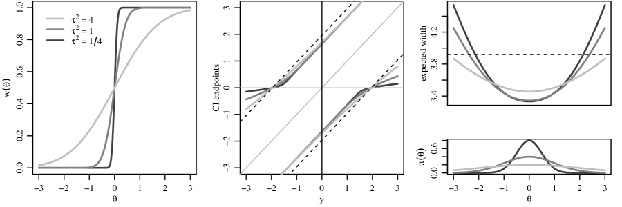
Figure 1: Descriptions of the FAB $z$-procedure. The left plot gives Bayes-optimal $w$-functions for three values of $\tau^{2}$, at level $\alpha=0.05$. The middle plot gives the corresponding confidence interval procedures, with the UMAU procedure given by dashed lines. The top plot on the right gives the risk functions (expected widths) of the 95% FAB $z$-intervals for the three values of $\tau^{2}$, with the corresponding prior densities plotted below.

2.2 FAB $t$-intervals

Adoption of Pratt’s $z$-interval has been limited, possibly due to two factors: First, in most applications the population variance is unknown, and second, the prior distribution for $\theta$ must be specified. We now address this first issue by developing a FAB $t$-interval. Suppose we have a sample $Y_{1},\ldots,Y_{n}\sim$ i.i.d. $N(\theta,\sigma^{2})$, with sufficient statistics $(\bar{Y},S^{2})$, the sample mean and (unbiased) sample variance. The standard UMAU $t$-interval is given by $\{\theta:\bar{y}+\tfrac{s}{\sqrt{n}}t_{\alpha/2}<\theta<\bar{y}+\tfrac{s}{\sqrt{n}}t_{1-\alpha/2}\}$. This interval is symmetric around $\bar{y}$, with the same tail-area probability ($\alpha/2$) defining the lower and upper endpoints. The development of the $w$-function described in the previous subsection suggests viewing the UMAU $t$-interval as belonging to the larger class of CRPs, given by

$$C_{w}(\bar{y},s^{2}) =\{\theta:\bar{y}+\tfrac{s}{\sqrt{n}}t_{\alpha(1-w(\theta))}<\theta<\bar{y}+\tfrac{s}{\sqrt{n}}t_{1-\alpha w(\theta)}\},$$ (4)

for some $w:\mathbb{R}\rightarrow(0,1)$. Any procedure thus defined satisfies $\Pr(\theta\in C_{w}(\bar{Y},S^{2})|\theta)=1-\alpha$ for any value of $\theta$. Additionally, $C_{w}$ is a CIP as long as $w$ is a continuous nondecreasing function:

Lemma 2.3.

Let $w:\mathbb{R}\rightarrow(0,1)$ be a continuous nondecreasing function. Then the set $C_{w}(\bar{y},s^{2})=\{\theta:\bar{y}+\tfrac{s}{\sqrt{n}}t_{\alpha(1-w(\theta))}<\theta<\bar{y}+\tfrac{s}{\sqrt{n}}t_{1-\alpha w(\theta)}\}$ is an interval and can be written as $(\theta^{L},\theta^{U})$, where $\theta^{L}$ and $\theta^{U}$ are solutions to $\theta^{L}=\bar{y}+\tfrac{s}{\sqrt{n}}t_{\alpha(1-w(\theta^{L}))}$ and $\theta^{U}=\bar{y}+\tfrac{s}{\sqrt{n}}t_{1-\alpha w(\theta^{U})}$.

For a given $w$-function, the endpoints of the interval can be reëxpressed as

$$F\left(\frac{\bar{y}-\theta^{U}}{s/\sqrt{n}}\right) =\alpha w(\theta^{U})$$ (5)

$$F\left(\frac{\bar{y}-\theta^{L}}{s/\sqrt{n}}\right) =1-\alpha(1-w(\theta^{L})),$$ (6)

where $F$ is the CDF of the $t_{n-1}$ distribution. Using the same logic as at the beginning of Section 2, the Bayes risk of a CRP for a prior distribution $\pi$ on $\theta$ and $\sigma^{2}$ is $R(\pi,C)=\int\Pr((\bar{Y},S^{2})\in A(\theta^{\prime}))\,d\theta^{\prime}$, where $\Pr((\bar{Y},S^{2})\in A(\theta^{\prime}))$ is the prior predictive (marginal) probability of $(\bar{Y},S^{2})$ being in the acceptance region $A(\theta^{\prime})$ under the prior distribution $\pi$. Given a prior $\pi$ that corresponds to a continuous, nondecreasing $w$-function, the Bayes-optimal FAB interval can be obtained numerically by using an iterative algorithm to solve (5) and (6). However, this requires computation of the $w$-function, which for each $\theta$ is the minimizer in $w$ of $\Pr((\bar{Y},S^{2})\in A_{w}(\theta))$, where

$$A_{w}(\theta)=\left\{(\bar{y},s^{2}):t_{\alpha w}<\frac{\bar{y}-\theta}{s/\sqrt{n}}<t_{1-\alpha(1-w)}\right\}.$$ (7)

Obtaining the optimal $w$-function will generally involve numerical integration. Consider a $N(\mu,\tau^{2})$ prior on $\theta$ and so conditionally on $\sigma^{2}$ we have $\bar{Y}\sim N(\mu,\sigma^{2}/n+\tau^{2})$ and $(n-1)S^{2}/\sigma^{2}\sim\chi^{2}_{n-1}$. From this we can show that $c(\bar{Y}-\theta)/(S/\sqrt{n})$ has a noncentral $t_{n-1}$ distribution with noncentrality parameter $\lambda=c\tfrac{\mu-\theta}{\sigma/\sqrt{n}}$, where $c=\sqrt{\sigma^{2}/n}/\sqrt{\sigma^{2}/n+\tau^{2}}$. Therefore, the probability of the event $\{(\bar{Y},S^{2})\in A(\theta)\}$, conditional on $\sigma^{2}$, can be written as

$$\Pr(\{\bar{Y},S^{2}\}\in A(\theta)|\sigma^{2})=F_{\lambda}(ct_{1-\alpha(1-w)})-F_{\lambda}(ct_{\alpha w}),$$

where $F_{\lambda}$ is the CDF of the noncentral $t_{n-1}$ distribution with parameter $\lambda=c\tfrac{\mu-\theta}{\sigma/\sqrt{n}}$. The Bayes-optimal $w$-function is therefore given by

$$w_{\pi}(\theta)=\arg\min_{w}\int\left(F_{\lambda}(ct_{1-\alpha(1-w)})-F_{\lambda}(ct_{\alpha w})\right)p_{\pi}(\sigma^{2})\,d\sigma^{2},$$ (8)

where $p_{\pi}(\sigma^{2})$ is the prior density over $\sigma^{2}$.

In the replication material for this article we provide R-code for obtaining $w_{\pi}(\theta)$ and the corresponding Bayes-optimal $t$-interval $C_{\pi}(\bar{y},s^{2})$ for the class of priors where $\theta$ and $\sigma^{2}$ are a priori independently distributed as normal and inverse-gamma random variables. Here, we provide some descriptions of this FAB $t$-interval procedure for some parameter values that make the interval comparable to the $z$-interval from Section 2.1. Specifically, we consider the case that $n=10$, $1/\sigma^{2}\sim$ gamma$(1,10)$ and $\theta\sim N(0,\tau^{2})$ for $\tau^{2}\in\{1/4,1,4\}$. This makes the prior median of $\sigma^{2}$ near 10, and the variance of $\bar{Y}$ near 1 (and so the variance of $\bar{Y}$ here is comparable to the variance of $Y$ in Section 2.1). The left panel of Figure 2 gives the $w$-functions, which are very similar to those of the FAB $z$-procedure displayed in Figure 1, but with somewhat larger derivatives near $\mu$. The second panel gives the FAB $t$-intervals as functions of $\bar{y}$, with $s^{2}$ fixed at 10. Again, the intervals resemble the corresponding $z$-intervals, but are slightly wider due to the use of $t$-quantiles instead of $z$-quantiles. The effect of not knowing $\sigma^{2}$ is more noticeable in the plot of the risk functions, given in the right-upper plot. While the shapes of the risk functions are similar to those of the analogous $z$-intervals, the risks (expected widths) are larger due to the fact that the width of a $t$-interval is dependent on $S^{2}$, which is proportional to a $\chi^{2}_{9}$ random variable having non-trivial skew.

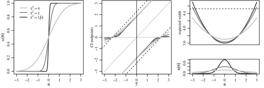
Figure 2: Descriptions of the FAB $t$-procedure. The left plot gives Bayes-optimal $w$-functions for three values of $\tau^{2}$, at level $\alpha=0.05$. The middle plot gives the corresponding confidence interval procedures with $s^{2}$ fixed at 10. The top plot on the right gives the expected widths of the 95% FAB $t$-intervals for the three values of $\tau^{2}$, with the corresponding prior densities plotted below.

3 Empirical FAB intervals for multigroup data

A potential obstacle to the adoption of FAB confidence intervals is the aversion that many researchers have to specifying a distribution over $\theta$. However, in multigroup data settings, probabilistic information about the mean $\theta_{j}$ of one group is may be obtained from data of the other groups. This information can be used to specify a probability distribution $\pi$ for the likely values of $\theta_{j}$, from which an empirical FAB interval may be constructed. Such an interval will have exact $1-\alpha$ coverage for every value of $\theta_{j}$, but a shorter expected width for values that are deemed likely by $\pi$. For the usual homoscedastic hierarchical normal model having a common within-group variance, we develop such a procedure that may be used in practice, and show that it is risk-optimal asymptotically in the number of groups. We also develop a similar procedure for the case of heteroscedastic groups.

3.1 Asymptotically optimal procedure for homoscedastic groups

Consider the case of $p$ normal populations with means $\theta_{1},\ldots,\theta_{p}$ and common variance and sample size, so that $Y_{1,j},\ldots Y_{n,j}\sim$ i.i.d. $N(\theta_{j},\sigma^{2})$ independently across groups (common sample sizes are used here solely to simplify notation). The standard hierarchical normal model posits that the heterogeneity across groups can be described by a normal distribution, so that $\theta_{1},\ldots,\theta_{p}\sim\text{i.i.d.}\,N(\mu,\tau^{2})$. In the multigroup setting, this normal distribution is not considered to be a prior distribution for a single $\theta_{j}$, but instead is a statistical model for the across-group heterogeneity of $\theta_{1},\ldots,\theta_{p}$. The parameters describing the across- and within-group heterogeneity are $\psi=(\mu,\tau^{2},\sigma^{2})$.

For each group $j$ let $C^{j}$ be a $1-\alpha$ CRP for $\theta_{j}$ that possibly depends on data from all of the other groups. Letting ${\boldsymbol{C}}=\{C^{1},\ldots,C^{p}\}$ we define the risk of such a multigroup confidence procedure as

$$R({\boldsymbol{C}},\psi)=\frac{1}{p}\sum_{j=1}^{p}{\text{E}}[|C^{j}({\boldsymbol{Y}})|],$$

where ${\boldsymbol{Y}}$ is the data from all of the groups and the expectation is over both ${\boldsymbol{Y}}$ and $\theta_{1},\ldots,\theta_{p}$. Under the hierarchical normal model, the risk at a value of $\psi$ is minimized by letting each $C^{j}$ be equal to $C_{w_{\psi}}(\bar{y}_{j})$, the FAB $z$-interval defined in Section 2 but with $\psi=(\mu,\tau^{2},\sigma^{2}/n)$, since ${\text{Var}}[\bar{Y}_{j}|\theta_{j}]=\sigma^{2}/n$. The oracle multigroup confidence procedure is then ${{\boldsymbol{C}}}_{w_{\psi}}=\{C_{w_{\psi}}(\bar{y}_{1}),\ldots,C_{w_{\psi}}(\bar{y}_{p})\},$ which has risk

$$R({{\boldsymbol{C}}}_{w_{\psi}},\psi)=\frac{1}{p}\sum_{j=1}^{p}{\text{E}}[|C_{w_{\psi}}(\bar{y}_{j})|]={\text{E}}[|C_{w_{\psi}}(\bar{y})|],$$

where $\bar{y}\sim N(\theta,\sigma^{2}/n)$ and $\theta\sim N(\mu,\tau^{2})$. While this oracle procedure is generally unavailable in practice, estimates of $\psi$ may be obtained from the data and used to construct a multigroup CIP that achieves the oracle risk asymptotically as $p\rightarrow\infty$. To show how to do this, we first construct a $1-\alpha$ CIP for a single $\theta$ based on $\bar{Y}\sim N(\theta,\sigma^{2}/n)$ and independent estimates $S^{2}$ and $\hat{\psi}$ of $\sigma^{2}$ and $\psi$. We show how the risk of this CIP converges to the oracle risk as $S^{2}\stackrel{{\scriptstyle a.s.}}{{\rightarrow}}\sigma^{2}$ and $\hat{\psi}\stackrel{{\scriptstyle a.s.}}{{\rightarrow}}\psi$, and then show how to use this fact to construct an asymptotically optimal multigroup CIP.

The ingredients of our FAB CIP for a single population mean $\theta$ are as follows: Let $\bar{Y}\sim N(\theta,\sigma^{2}/n)$ and $qS^{2}/\sigma^{2}\sim\chi^{2}_{q}$ be independent. Consider the $1-\alpha$ CRP for $\theta$ given by

$$C_{w}(\bar{y},s^{2})=\{\theta:\bar{y}+\tfrac{s}{\sqrt{n}}t_{\alpha(1-w(\theta))}<\theta<\bar{y}+\tfrac{s}{\sqrt{n}}t_{1-\alpha w(\theta)}\},$$ (9)

where the $t$-quantiles are those of the $t_{q}$-distribution. As described in Section 2.2, this procedure has $1-\alpha$ coverage for every value of $\theta$ and is an interval if $w:\mathbb{R}\rightarrow(0,1)$ is a continuous nondecreasing function. This holds for non-random $w$-functions as well as for random $w$-functions that are independent of $\bar{Y}$ and $S^{2}$. In particular, suppose we have estimates $\hat{\psi}=(\hat{\mu},\hat{\tau}^{2},\hat{\sigma}^{2}/n)$ that are independent of $\bar{Y}$ and $S^{2}$. We can then let $w=w_{\hat{\psi}}$, the $w$-function of the Bayes optimal $z$-interval assuming a prior distribution $\theta\sim N(\hat{\mu},\hat{\tau}^{2})$ and that ${\text{Var}}[\bar{Y}|\theta]=\hat{\sigma}^{2}/n$. Note that we are not assuming $(\mu,\tau^{2},\sigma^{2}/n)$ actually equals $(\hat{\mu},\hat{\tau}^{2},\hat{\sigma}^{2}/n)$, we are just using these values to approximate the optimal $w$-function by $w_{\hat{\psi}}$ and the optimal CIP by $C_{w_{\hat{\psi}}}$.

The random interval $C_{w_{\hat{\psi}}}(\bar{Y},S^{2})$ differs from the optimal interval $C_{w_{\psi}}(\bar{Y})$ in three ways: First, the former uses $S^{2}$ instead of $\sigma^{2}$ to scale the endpoints of the interval. Second, the former uses $t$-quantiles instead of standard normal quantiles. Third, the former uses $\hat{\psi}$ to define the $w$-function, instead of $\psi$. Now as $q$ increases, $S^{2}\stackrel{{\scriptstyle a.s.}}{{\rightarrow}}\sigma^{2}$ and the $t$-quantiles in (9) converge to the corresponding $z$-quantiles. If we are also in a scenario where $\hat{\psi}$ can be indexed by $q$ and $\hat{\psi}\stackrel{{\scriptstyle a.s.}}{{\rightarrow}}\psi$, then we expect that $w_{\hat{\psi}}$ converges to $w_{\psi}$ and that the risk of $C_{w_{\hat{\psi}}}$ converges to the oracle risk:

Proposition 3.1.

Let $\bar{Y}\sim N(\theta,\sigma^{2}/n)$, $qS^{2}/\sigma^{2}\sim\chi^{2}_{q}$, and $\hat{\psi}$ be independent for each value of $q$, with $\hat{\psi}\stackrel{{\scriptstyle a.s.}}{{\rightarrow}}\psi$ as $q\rightarrow\infty$. Then

1. $C_{w_{\hat{\psi}}}$ defined in (9) is a $1-\alpha$ CIP for each value of $\theta$ and $q$;

2. ${\text{E}}[|C_{w_{\hat{\psi}}}|]\rightarrow{\text{E}}[|C_{w_{\psi}}|]$ as $q\rightarrow\infty$.

We now return to the problem of constructing an asymptotically optimal multigroup procedure. Let $\bar{Y}_{j}$ and $S^{2}_{j}$ be the sample mean and variance for a given group $j$. Divide the remaining groups into two sets, with $p_{1}-1$ in the first set and $p_{2}=p-p_{1}+1$ in the second. Pool the group-specific sample variances of the first set of groups with $S_{j}^{2}$ to obtain an estimate $\tilde{S}^{2}_{j}$ of $\sigma^{2}$, so that $p_{1}(n-1)\tilde{S}^{2}_{j}/\sigma^{2}\sim\chi^{2}_{p_{1}(n-1)}$. From the remaining groups, obtain a strongly consistent estimate $\hat{\psi}_{j}$ of $\psi$ (such as the MLE or a moment-based estimate). Then $\bar{Y}_{j}$, $\tilde{S}^{2}_{j}$ and $\hat{\psi}_{j}$ are independent for each value of $p$. Therefore, a $1-\alpha$ CIP for $\theta_{j}$ is given by

$$C_{w_{\hat{\psi}_{j}}}(\bar{y}_{j},\tilde{s}_{j}^{2})=\{\theta_{j}:\bar{y}_{j}+\tfrac{\tilde{s}_{j}}{\sqrt{n}}t_{\alpha(1-w_{\hat{\psi}_{j}}(\theta_{j}))}<\theta_{j}<\bar{y}_{j}+\tfrac{\tilde{s}_{j}}{\sqrt{n}}t_{1-\alpha w_{\hat{\psi}_{j}}(\theta_{j})}\},$$ (10)

where the quantiles are those of the $t_{p_{1}(n-1)}$ distribution. If $p_{1}$ is chosen so that it remains a fixed fraction of $p$ as $p$ increases, then $\tilde{S}^{2}_{j}$ and $\hat{\psi}_{j}$ converge to $\sigma^{2}$ and $\psi$ respectively, and the $t$-quantiles converge to the corresponding standard normal quantiles. By Proposition 3.1, the risk of this interval converges to that of the oracle risk. Repeating this construction for each group $j$ results in a multigroup confidence procedure that has $1-\alpha$ coverage for each group conditional on $(\theta_{1},\ldots,\theta_{p})$, but is also asymptotically optimal on average across the $N(\mu,\tau^{2})$ population of $\theta$-values.

In practice for finite $p$, different choices of $p_{1}$ and $p_{2}$ will affect the resulting confidence intervals. Since the minimal width of each interval is directly tied to the degrees of freedom $p_{1}(n-1)$ of the variance estimate $\tilde{S}_{j}^{2}$, we suggest choosing $p_{1}$ to ensure that the quantiles of the $t_{p_{1}(n-1)}$ distribution are reasonably close to those of the standard normal distribution. If either $p$ or $n$ are large, this can be done while still allowing $p_{2}$ to be large enough for $(\hat{\mu},\hat{\tau}^{2},\hat{\sigma}^{2}/n)$ to be useful.

3.2 A procedure for heteroscedastic groups

If a researcher is unwilling to assume a common within-group variance, constant $1-\alpha$ group-specific coverage can still be ensured by using intervals of the form

$$C_{w_{j}}(\bar{y}_{j},s^{2}_{j})=\{\theta_{j}:\bar{y}_{j}+\tfrac{s_{j}}{\sqrt{n_{j}}}t_{\alpha(1-w_{j}(\theta_{j}))}<\theta_{j}<\bar{y}_{j}+\tfrac{s_{j}}{\sqrt{n_{j}}}t_{1-\alpha w_{j}(\theta_{j})}\},$$ (11)

where $w_{j}$ is an estimate of the Bayes-optimal $w$-function discussed at the end of Section 2.2, estimated with data from groups other than $j$. We recommend obtaining $w_{j}$ from a hierarchical model for both the group-specific means and variances, as this allows across-group sharing of information about both of these quantities. For example, the replication material for this article provides code to obtain estimates of the $w$-function that is optimal for the following model of across-group heterogeneity:

$$\theta_{1},\ldots,\theta_{p} \sim\text{i.i.d.}\ N(\mu,\tau^{2})$$ (12)

$$1/\sigma_{1}^{2},\ldots,1/\sigma_{p}^{2} \sim\text{i.i.d.}\ \text{gamma}(a,b).$$

We estimate the across-group heterogeneity parameters $(\mu,\tau^{2},a,b)$ as follows: For each group $j$ let $X_{j}^{2}=\sum_{i}(Y_{i,j}-\bar{Y}_{j})^{2}\sim\sigma^{2}_{j}\chi^{2}_{n_{j}-1}$. If $1/\sigma^{2}_{j}\sim\text{gamma}(a,b)$ independently for each $j$ then the marginal density of $X_{1}^{2},\ldots,X_{p}^{2}$ can be shown to be

$$p(x_{1}^{2},\ldots,x_{p}^{2}|a,b)\prod_{j=1}^{p}c(x^{2}_{j})\frac{\Gamma(a+(n_{j}-1)/2)b^{a}}{\Gamma(a)(b+x^{2}_{j}/2)^{a+(n_{j}-1)/2}},$$

where $c$ is a function that does not depend on $a$ or $b$. This quantity can be maximized to obtain marginal maximum likelihood estimates of $\hat{a}$ and $\hat{b}$. Now if $\sigma^{2}_{1},\ldots,\sigma^{2}_{p}$ were known, then a maximum likelihood estimate of $(\mu,\tau^{2})$ could be obtained based on the fact that under the hierarchical model, $\bar{Y}_{j}\sim N(\mu,\sigma^{2}_{j}/n_{j}+\tau^{2})$ independently across groups. Since the $\sigma^{2}_{j}$’s are not known we use empirical Bayes estimates, given by $\hat{\sigma}^{2}_{j}=(\hat{b}+x_{j}^{2}/2)/(\hat{a}+(n_{j}-1)/2)$, to obtain the “plug-in” marginal likelihood estimates $(\hat{\mu},\hat{\tau}^{2})$:

$$(\hat{\mu},\hat{\tau}^{2})=\arg\max_{\mu,\tau^{2}}\prod_{j}\frac{1}{\sqrt{\hat{\sigma}^{2}_{j}/n_{j}+\tau^{2}}}\phi\left(\frac{\bar{y}_{j}-\mu}{\sqrt{\hat{\sigma}^{2}_{j}/n_{j}+\tau^{2}}}\right),$$

where $\phi$ is the standard normal probability density function.

To create a FAB $t$-interval for a given group $j$, we obtain estimates $(\hat{\mu}_{j},\hat{\tau}^{2}_{j},\hat{a}_{j},\hat{b}_{j})$ using the procedure described above with data from all groups except group $j$. The $w$-function $w_{j}$ for group $j$ is taken to be the Bayes-optimal $w$-function defined by Equation 8, under the estimated prior $\theta_{j}\sim N(\hat{\mu}_{j},\hat{\tau}^{2}_{j})$ and $1/\sigma^{2}_{j}\sim\text{gamma}(\hat{a}_{j},\hat{b}_{j})$. The independence of $(\bar{Y}_{j},S^{2}_{j})$ and $(\hat{\mu}_{j},\hat{\tau}^{2}_{j},\hat{a}_{j},\hat{b}_{j})$ ensures that the resulting FAB $t$-interval has exact $1-\alpha$ coverage, conditional on $\theta_{1},\ldots,\theta_{p}$ and $\sigma_{1}^{2},\ldots,\sigma_{p}^{2}$.

We speculate that this procedure enjoys similar optimality properties to those of the approach for homoscedastic groups described in Section 3.1: If the hierarchical model given by (12) is correct, then as the number $p$ of groups increases, the estimates $(\hat{\mu}_{j},\hat{\tau}^{2}_{j},\hat{a}_{j},\hat{b}_{j})$ will converge to $(\mu,\tau^{2},a,b)$ and the interval for a given group will converge to the corresponding Bayes-optimal interval. So far we have been unable to prove this, the primary difficulty being that the Bayes-optimal $w$ function given by Equation 8 is a non-standard integral involving the non-central $t$-distribution, and is not easily studied analytically.

4 Radon data example

A study by the U.S. Environmental Protection Agency measured radon levels in a random sample of homes. Price et al. (1996) use a subsample of these data to estimate county-specific mean radon levels (on a log scale) in the state of Minnesota. This dataset consists of log radon values measured in 919 homes, each being located in one of $p=85$ counties. County-specific sample sizes ranged from 1 to 116 homes. In this section we obtain a $95\%$ FAB confidence interval for each county-specific mean radon level, based on data from all of the counties, and compare these intervals to the corresponding UMAU intervals. Also, in a simulation study based on these data, we compare the expected widths of these two types of intervals to empirical Bayes posterior intervals, and show how the latter do not provide constant coverage across values of the county-specific means.

4.1 County-specific confidence intervals

Letting $Y_{i,j}$ be the radon measurement for home $i$ in county $j$, we assume throughout this section that $Y_{1,j}\ldots,Y_{n_{j},j}\sim$ i.i.d. $N(\theta_{j},\sigma^{2}_{j})$ and that the data are independently sampled across counties. Under the assumptions of a constant across-county variance and the normal hierarchical model $\theta_{1},\ldots,\theta_{p}\sim$ i.i.d. $N(\mu,\tau^{2})$, the maximum likelihood estimates of $\sigma^{2}$, $\mu$ and $\tau^{2}$ are $\hat{\sigma}^{2}=0.637$, $\hat{\mu}=1.313$ and $\hat{\tau}^{2}=0.096$. The estimate of the across-county variability is substantially smaller than the estimate of within-county variability, suggesting that there is useful information to be shared across the groups. However, Levene’s test of heteroscedasticity (an $F$-test using the absolute difference between the data and group-specific medians) rejects the null of homoscedasticity with a $p$-value of 0.011. For this reason, we use the FAB $t$-interval procedure described in Section 3.2 for each group, having the form $\{\theta_{j}:\bar{y}_{j}+\sqrt{s^{2}_{j}/n_{j}}\times t_{\alpha(1-w_{j}(\theta_{j}))}<\theta_{j}<\bar{y}_{j}+\sqrt{s^{2}_{j}/n_{j}}\times t_{1-\alpha w_{j}(\theta_{j})}\}$, where $\alpha=.05$, $\bar{y}_{j}$ and $s^{2}_{j}$ are the sample mean and variance from county $j$, and $w_{j}$ is the optimal $w$-function assuming $\theta_{j}\sim N(\hat{\mu}_{j},\hat{\tau}^{2}_{j})$ and $1/\sigma^{2}_{j}\sim$ gamma$(\hat{a}_{j},\hat{b}_{j})$, where $\hat{\mu}_{j},\hat{\tau}^{2}_{j},\hat{a}_{j}$ and $\hat{b}_{j}$ are estimated from the counties other than county $j$. Such intervals have 95% coverage for each county, assuming only within-group normality.

We constructed FAB and UMAU intervals for each county that had a sample size greater than one, i.e. counties for which we could obtain an unbiased within-sample variance estimate. Intervals for counties with sample sizes greater than two are displayed in Figure 3 (intervals based on a sample size of two were excluded from the figure because their widths make smaller intervals difficult to visualize). The UMAU intervals are wider than the FAB intervals for 77 of the 82 counties having a sample size greater than 1, and are 30% wider on average across counties. Generally speaking, the counties for which the FAB intervals provide the biggest improvement are those with smaller sample sizes and sample means near the across-group average. Conversely, the five counties for which the UMAU intervals are narrower than the FAB interval are those with moderate to large sample sizes, and sample means somewhat distant from the across-group average.

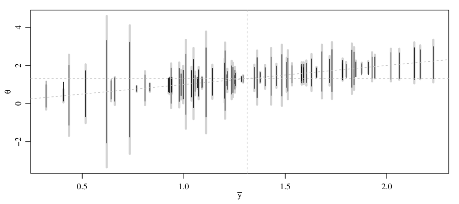
Figure 3: FAB and UMAU 95% confidence intervals for the radon dataset. The UMAU intervals are plotted as wide gray lines, the FAB intervals as narrow black lines. Vertical and horizontal lines are drawn at $\sum\bar{y}_{j}/p$.

4.2 Risk performance and comparison to posterior intervals

Assuming within-group normality, the FAB interval procedure described above has 95% coverage for each group $j$ and for all values of $\theta_{1},\ldots,\theta_{p}$. Furthermore, the procedure is designed to approximately minimize the expected risk under the hierarchical model $\theta_{1},\ldots,\theta_{p}\sim$ i.i.d. $N(\mu,\tau^{2})$, among all $95\%$ CRPs. However, one may wonder how well the FAB procedure works for fixed values of $\theta_{1},\ldots,\theta_{p}$. This question is particularly relevant in cases where the hierarchical model is misspecified, or if a hierarchical model is not appropriate (e.g., if the groups are not sampled). We investigate this for the radon data with a simulation study in which we take the county-specific sample means and variances as the true county-specific values, that is, we set $\theta_{j}=\bar{y}_{j}$ and $\sigma^{2}_{j}=s_{j}^{2}$ for each county $j$. We then simulate $n_{j}$ observations for each county $j$ from the model $Y_{1,j},\ldots,Y_{n_{j},j}\sim$ i.i.d. $N(\theta_{j},\sigma^{2}_{j})$.

We generated 10,000 such simulated datasets. For each dataset, we computed the widths of the 95% FAB and UMAU confidence intervals for each county having a sample size greater than one. Additionally, for comparison we also computed empirical Bayes posterior intervals, which are often used in hierarchical modeling. The posterior interval for group $j$ is given by $\hat{\theta}_{j}\pm t_{1-\alpha/2}\times(1/\hat{\tau}^{2}+n_{j}/\hat{s}^{2}_{j})^{-1/2}$, where $\hat{\theta}_{j}$ is the empirical Bayes estimator given by

$$\hat{\theta}_{j}=\frac{\hat{\mu}/\hat{\tau}^{2}+\bar{y}_{j}n_{j}/s_{j}^{2}}{1/\hat{\tau}^{2}+n_{j}/s_{j}^{2}},$$

and $t_{1-\alpha/2}$ is the $1-\alpha/2$ quantile of the $t_{n-1}$-distribution. As discussed in the Introduction, such intervals are always narrower than the corresponding UMAU intervals but will not have $1-\alpha$ frequentist coverage for each group. Instead, such intervals generally have $1-\alpha$ coverage on average, or in expectation with respect to the hierarchical model over the $\theta_{j}$’s.

The results of this simulation study are displayed in Figure 4. The left panel of the figure gives the expected widths of the FAB and Bayes procedures relative to those of the UMAU procedure. Based on the 10,000 simulated datasets, the estimated expected widths across counties were about 2.28, 1.60 and 1.61, respectively for the UMAU, FAB and Bayes procedures respectively. As with the actual interval widths for the non-simulated data, expected widths of the FAB intervals are smaller than those of the UMAU intervals for most counties (79 out of 82). The Bayes intervals are always narrower than the UMAU intervals for all groups by construction. However, while they tend to be narrower than the FAB intervals for $\theta_{j}$’s far from $\bar{\theta}=\sum\theta_{j}/p$, near this average they are often wider than the FAB intervals. This is not too surprising - the FAB intervals are at their narrowest near this overall average, while the Bayes intervals tend to over-cover here. This latter issue is illustrated in the right panel of the figure, which shows how the Bayes credible intervals do not have constant coverage across groups. This is because the Bayes intervals are centered around biased estimates that are shrunk towards the estimated overall mean $\bar{\theta}$. If $\theta_{j}$ is far from $\bar{\theta}$ then the bias is high and the coverage is too low, whereas if $\theta_{j}$ is near $\bar{\theta}$ the coverage is too high since the variability of the shrinkage estimate $\hat{\theta}_{j}$ is lower than that of $\bar{y}_{j}$. The group-specific coverage rates of the Bayes intervals vary from about 91% to 98%, although the average coverage rate across groups is approximately 95%. In summary, the UMAU procedure provides constant $1-\alpha$ coverage across groups, but wider intervals than those obtained from the FAB and Bayes procedures. The Bayes procedure provides narrower intervals but non-constant coverage. The FAB procedure provides both narrower intervals and constant coverage.

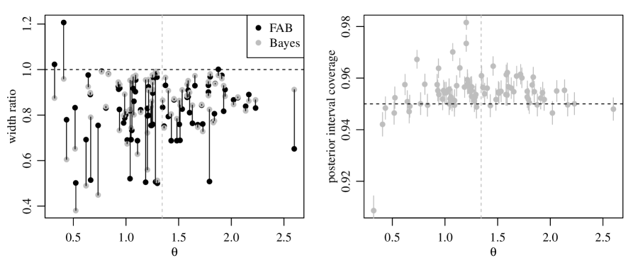
Figure 4: Simulation results. The left panel gives relative expected interval widths of the FAB and Bayes procedures relative to the UMAU procedure. The right panel indicates how coverage rates of Bayes posterior intervals are not constant across groups. Points are coverage rates based on 10,000 simulated datasets, and vertical lines are nominal 95% intervals representing Monte Carlo standard error. Vertical lines are drawn at $\sum\theta_{j}/p$ in each panel.

5 Discussion

Standard analyses of multilevel data utilize multigroup confidence interval procedures that either have constant coverage but do not share information across groups, or share information across groups but lack constant coverage. These latter procedures typically do maintain a pre-specified coverage rate on average across groups, but the value of this property is unclear if one wants to make group-specific inferences. The FAB procedures developed in this article have coverage rates that are constant in the mean parameter, and so maintain constant coverage for each group selected into the dataset, while also making use of across-group information. The FAB procedures are approximately optimal among constant coverage procedures if the across-group heterogeneity is well-represented by a normal hierarchical model.

If the across-group heterogeneity is not well-represented by a hierarchical normal model, then the FAB procedure will still maintain the chosen constant coverage rate but may not be optimal. We speculate that in such cases, the FAB procedure based on a hierarchical normal model, while not optimal, will still have better risk than the UMAU procedure when the across-group heterogeneity corresponds to any probability distribution with a finite second moment. This is partly because the UMAU procedure is a limiting case of the FAB procedure as the across-group variance goes to infinity. We have developed an analytical argument of this and have gathered computational evidence, but a complete proof of the dominance of a misspecified FAB procedure over the UMAU procedure is still a work in progress. Of course, the basic idea behind the FAB procedure could be implemented with alternative models describing across-group heterogeneity, such as models that allow for sparsity among the group-level parameters. We have implemented a few such procedures computationally, but studying them analytically is challenging.

Replication code for this article can be found at the second author’s website. The multigroup FAB procedures discussed in Sections 3 and 4 are provided by the R-package fabCI.

Appendix: Proofs

Proof of Lemma 2.1.

This lemma follows from Ferguson (1967, Section 5.3), which says that for any level-$\alpha$ test of a point null hypothesis for a one-parameter exponential family, there exists a two-sided test of equal or greater power. Let $\{\tilde{\phi}_{\theta}(y):\theta\in\mathbb{R}\},\{\tilde{A}(\theta):\theta\in\mathbb{R}\}$ be the test functions and acceptance regions corresponding to the CRP $\tilde{C}(y)$. The coverage of $\tilde{C}$ is

$$\Pr(Y\in\tilde{A}(\theta)|\theta)=1-{\text{E}}[\tilde{\phi}_{\theta}(Y)|\theta].$$ (13)

By Theorem 2 from Ferguson (1967, Section 5.3), for each $\theta\in\mathbb{R}$ there exists a two-sided test $\phi_{\theta}$ such that

$${\text{E}}[\phi_{\theta}(Y)|\theta]={\text{E}}[\tilde{\phi}_{\theta}(Y)|\theta].$$ (14)

Denote the acceptance regions corresponding to these two-sided test as $\{A(\theta):\theta\in\mathbb{R}\}$. Inverting these regions gives a CIP $C(y)$. The coverage of $C(y)$ is

$$\Pr(Y\in A(\theta)|\theta)=1-{\text{E}}[\phi_{\theta}(Y)|\theta].$$ (15)

Hence by (13), (15), and (14), the coverage of $C(y)$ is the same as the coverage of $\tilde{C}(y)$. The width of $\tilde{C}(y)$ is:

$$W(y)=\int_{\mathbb{R}}1(t\in\tilde{C}(y))dt=\int_{\mathbb{R}}1(y\in\tilde{A}(t))dt=\int_{\mathbb{R}}(1-\tilde{\phi}_{t}(y))dt.$$

The expected width of $\tilde{C}(y)$ is:

$${\text{E}}[\tilde{W}|\theta]=\int_{\mathbb{R}}W(y)p(y|\theta)dy=\int_{\mathbb{R}}\int_{\mathbb{R}}(1-\tilde{\phi}_{t}(y))p(y|\theta)dydt$$ (16)

where $p(y|\theta)$ is the density of $Y$ given $\theta$. Similarly, the expected width of $C(y)$ is

$${\text{E}}[W|\theta]=\int_{\mathbb{R}}\int_{\mathbb{R}}(1-\phi_{t}(y))p(y|\theta)dydt.$$ (17)

Again, by Theorem 2 from Ferguson (1967, Section 5.3), for every $\theta\in\mathbb{R}$

$$\int_{\mathbb{R}}\phi_{t}(y)p(y|\theta)dy\geq\int_{\mathbb{R}}\tilde{\phi}(y)p(y|\theta)dy.$$

Thus

$$\int_{\mathbb{R}}(1-\phi_{t}(y))p(y|\theta)dy\leq\int_{\mathbb{R}}(1-\tilde{\phi}_{t}(y))p(y|\theta)dy.$$ (18)

Therefore by (16), (17), (18), we have ${\text{E}}[W|\theta]\leq{\text{E}}[\tilde{W}|\theta]$. ∎

Proof of Proposition 2.1.

Without loss of generality, we prove the proposition for the simple case when $\mu=0$ and $\sigma^{2}=1$. Other cases can be obtained by reparametrizing as $\tilde{Y}=(Y-\mu)/\sigma$, $\tilde{\theta}=(\theta-\mu)/\sigma$ and $\tilde{\tau}^{2}=\tau^{2}/\sigma^{2}$ so that $\tilde{Y}\sim N(\tilde{\theta},1)$ and $\tilde{\theta}\sim N(0,\tilde{\tau}^{2})$.

The Bayes optimal procedure minimizes the Bayes risk $R(\psi,C_{w})=\int\Pr(Y\in A(\theta))\,d\theta$, where $Y$ has the marginal density $N(0,1+\tau^{2})$. For a given $w$-function, the Bayes risk is

$$R(\psi,C_{w}) =\int_{\mathbb{R}}\Phi(\frac{\theta-l}{\sqrt{1+\tau^{2}}})-\Phi(\frac{\theta-u}{\sqrt{1+\tau^{2}}})\ d\theta$$ (19)

$$=\int_{\mathbb{R}}\Phi(\frac{\theta-\Phi^{-1}(\alpha(1-w))}{\sqrt{1+\tau^{2}}})-\Phi(\frac{\theta-\Phi^{-1}(1-\alpha w)}{\sqrt{1+\tau^{2}}})\ d\theta.$$

We will show that, as a function of $w$, the integrand $H$ is minimized at $w_{\psi}(\theta)$ as given in the proposition statement. First, we obtain the derivative of $H$ with respect to $w$:

$$H^{\prime}(w)= \exp(-\frac{1}{2}\frac{(\theta-\Phi^{-1}(\alpha(1-w)))^{2}}{1+\tau^{2}})\frac{1}{\sqrt{1+\tau^{2}}}\frac{\alpha}{\exp(-\frac{1}{2}(\Phi^{-1}(\alpha(1-w)))^{2})}$$

$$-\exp(-\frac{1}{2}\frac{(\theta-\Phi^{-1}(1-\alpha w))^{2}}{1+\tau^{2}})\frac{1}{\sqrt{1+\tau^{2}}}\frac{\alpha}{\exp(-\frac{1}{2}(\Phi^{-1}(1-\alpha w))^{2})}.$$

Setting this to zero and simplifying shows that a critical point $w_{\psi}$ satisfies

$${2\theta}/{\tau^{2}}=\Phi^{-1}(w\alpha)-\Phi^{-1}((1-w)\alpha).$$ (20)

Let the right side of (20) be $g(w)$. It’s not difficult to verify that $g(w)$ a continuous and strictly increasing function of $w$, with range $(-\infty,\infty)$. Thus there is a unique solution $w_{\psi}(\theta)$ to the equation above, $w_{\psi}(\theta)=g^{-1}({2\theta/\tau^{2}})$, which is a continuous and strictly increasing function of $\theta$. Since $H^{\prime}(w)$ is continuous on $(0,1)$ with only one root, and $\lim_{w\rightarrow 0}\hskip 5.69046ptH^{\prime}(w)=-\infty$, $\lim_{w\rightarrow 1}\hskip 5.69046ptH^{\prime}(w)=\infty$, then $H(w)$ is minimized by $w_{\psi}(\theta)$. Therefore $w_{\psi}(\theta)$ minimizes the Bayes risk, and $C_{w_{\psi}}$ is the Bayes-optimal procedure among all CRPs. ∎

Proof of Lemma 2.2.

$C_{w}(y)$ can be written as $C_{w}(y)=\{\theta:y<\theta-\sigma l(\theta)\;\textrm{and}\;\theta-\sigma u(\theta)<y\}$. Letting $f_{1}(\theta)=\theta-\sigma u(\theta)$, $f_{2}(\theta)=\theta-\sigma l(\theta)$, we first prove that $C_{w}(y)$ can also be written as $C_{w}(y)=\{\theta:f_{2}^{-1}(y)<\theta\;\textrm{and}\;\theta<f_{1}^{-1}(y)\}$. Note that both $\Phi^{-1}$ and $w(\theta)$ are continuous nondecreasing functions. Therefore $f_{1}(\theta)=\theta-\Phi^{-1}(1-\alpha w(\theta))$ is a strictly increasing continuous function, with $\lim_{\theta\to-\infty}\theta-\Phi^{-1}(1-\alpha w(\theta))=-\infty$ and $\lim_{\theta\to+\infty}\theta-\Phi^{-1}(1-\alpha w(\theta))=+\infty.$ Hence, $f_{1}^{-1}$ exists, and is a strictly increasing continuous function with range $(-\infty,\infty)$. Thus $f_{1}(\theta)<y$ can also be expressed as $\theta<f_{1}^{-1}(y)$. Similarly, $y<f_{2}(\theta)$ can also be expressed as $f_{2}^{-1}(y)<\theta$. Next, in order to show that $C_{w}(y)$ is an interval, we need to show that $f_{2}^{-1}(y)<f_{1}^{-1}(y)$. To see this, we only need to show

$$\theta-\sigma\Phi^{-1}(1-\alpha w(\theta))<\theta-\sigma\Phi^{-1}(\alpha(1-w(\theta))),$$

or that $\Phi^{-1}(\alpha w(\theta))<\Phi^{-1}(1-\alpha(1-w(\theta)))$. This follows since $\Phi^{-1}(x)$ is a strictly increasing function. Thus $C_{w}(y)=\{\theta:f_{2}^{-1}(y)<\theta<f_{1}^{-1}(y)\}$, which is an interval. ∎

Proof of Lemma 2.3.

The proof is basically the same as the proof of Lemma 2.2. We only need to replace $y$ with $\bar{y}$, $\sigma$ with $s/\sqrt{n}$, and the $z$-quantiles with $t$-quantiles, and then use the same logic as in the proof of Lemma 2.2. ∎

The proof of Proposition 3.1 requires the following lemma that bounds the width of the FAB $t$-interval:

Lemma.

The width of $C_{w_{\psi}}(\bar{y},s^{2})$ satisfies

$$|C_{w_{\psi}}(\bar{y},s^{2})|<|\bar{y}-\mu|+\tfrac{s}{\sqrt{n}}(|t(\alpha/2)|+|t(1-\alpha/2)|),$$ (21)

where $t$-quantiles are those of the $t_{q}$-distribution.

Proof.

For notational convenience, for this proof and the proof of Proposition 3.1, we write $t_{\alpha}$ as $t(\alpha)$. By previous results, the endpoints $\theta^{L}$ and $\theta^{U}$ of $C_{w_{\psi}}(\bar{y},s^{2})$ are solutions to

$$\begin{array}[]{l}\theta^{U}-\tfrac{s}{\sqrt{n}}t(1-\alpha w_{\psi}(\theta^{U}))=\bar{y}\\ \theta^{L}-\tfrac{s}{\sqrt{n}}t(\alpha(1-w_{\psi}(\theta^{L})))=\bar{y}.\\ \end{array}$$ (22)

Here $w_{\psi}(\theta)$ is defined as $w_{\psi}(\theta)=g^{-1}(\tfrac{2(\theta-\mu)}{{\tau}^{2}/\sigma})$, where $g(w)=\Phi^{-1}(\alpha w)-\Phi^{-1}(\alpha(1-w))$. At the upper endpoint, we have $w_{\psi}(\theta^{U})=F((\bar{y}-\theta^{U})/(s/\sqrt{n}))/\alpha$, where $F$ is the CDF of the $t_{q}$-distribution. When $\theta^{U}>\mu$, we have $w_{\psi}(\theta^{U})>g^{-1}(0)=1/2$. Thus $\theta^{U}<\bar{y}-\tfrac{s}{\sqrt{n}}t(\alpha/2)$. Also, $g^{-1}(\tfrac{2(\theta^{U}-\mu)}{\tau^{\prime 2}/\sigma})<1$, so $\theta^{U}>\bar{y}-\tfrac{s}{\sqrt{n}}t(\alpha)$. When $\theta^{U}<\mu$, $\bar{y}-\tfrac{s}{\sqrt{n}}t(\alpha/2)<\theta^{U}$. This implies that

$$\bar{y}-\tfrac{s}{\sqrt{n}}t(\alpha)<\theta^{U}<\bar{y}-\tfrac{s}{\sqrt{n}}t(\alpha/2) \ \text{if}\ \theta^{U}>\mu$$

$$\bar{y}-\tfrac{s}{\sqrt{n}}t(\alpha/2)<\theta^{U}<\mu \ \text{if}\ \theta^{U}<\mu.$$

Similarly we have

$$\mu<\theta^{L}<\bar{y}-\tfrac{s}{\sqrt{n}}t(1-\alpha/2) \ \text{if}\ \theta^{L}>\mu$$

$$\bar{y}-\tfrac{s}{\sqrt{n}}t(1-\alpha/2)<\theta^{L}<y-\tfrac{s}{\sqrt{n}}t(1-\alpha) \ \text{if}\ \theta^{L}<\mu.$$

Therefore

$$|C_{w_{\psi}}(\bar{y},s)|=\theta^{U}-\theta^{L}<|\bar{y}-\mu|+\tfrac{s}{\sqrt{n}}(|t(\alpha/2)|+|t(1-\alpha/2)|).$$

∎

Proof of Proposition 3.1.

That $C_{w_{\hat{\psi}}}$ is a $1-\alpha$ CIP follows by construction of the interval and that $\hat{\psi}$ is independent of $\bar{Y}$ and $S^{2}$. To prove the convergence of the risk, we denote the endpoints of the oracle CIP $C_{w_{\psi}}$ as $\theta^{U}$ and $\theta^{L}$, which are the solutions to

$$\begin{array}[]{l}\theta^{U}-\tfrac{\sigma}{\sqrt{n}}\Phi^{-1}(1-\alpha w_{\psi}(\theta^{U}))=\bar{Y}\\ \theta^{L}-\tfrac{\sigma}{\sqrt{n}}\Phi^{-1}(\alpha(1-w_{\psi}(\theta^{L})))=\bar{Y}.\\ \end{array}$$

We denote the endpoints of $C_{w_{\hat{\psi}}}$ as $\theta^{U}_{q}$ and $\theta^{L}_{q}$, which are the solutions to

$$\begin{array}[]{l}\theta^{U}_{q}-\tfrac{S}{\sqrt{n}}t(1-\alpha w_{\hat{\psi}}(\theta^{U}_{q}))=\bar{Y}\\ \theta^{L}_{q}-\tfrac{S}{\sqrt{n}}t(\alpha(1-w_{\hat{\psi}}(\theta^{L}_{q})))=\bar{Y}.\\ \end{array}$$

We first prove that $|C_{w_{\hat{\psi}}}|-|C_{w_{\psi}}|=(\theta^{U}_{q}-\theta^{U})+(\theta^{L}-\theta^{L}_{q})\stackrel{{\scriptstyle a.s.}}{{\rightarrow}}0$ as $q\to\infty$ for each fixed $\bar{Y}$. We can write the upper endpoints as $\theta^{U}=G(\psi,\bar{Y},\sigma^{2})$, and $\theta^{U}_{q}=G_{q}(\hat{\psi},\bar{Y},S^{2})$, where $G$ and $G_{q}$ are continuous functions of their parameters. The difference between $G$ and $G_{q}$ is that the former is obtained based on $z$-quantiles, while the later is based on $t$-quantiles. We have

$$|\theta^{U}_{q}-\theta^{U}| =|G_{q}(\hat{\psi},\bar{Y},S^{2})-G(\psi,\bar{Y},\sigma^{2})|$$ (23)

$$\leq|G_{q}(\hat{\psi},\bar{Y},S^{2})-G(\hat{\psi},\bar{Y},S^{2})|+|G(\hat{\psi},\bar{Y},S^{2})-G(\psi,\bar{Y},\sigma^{2})|.$$ (24)

The first term in (24) converges to zero because the convergence of $G_{q}\to G$ is uniform, and the second term converges to zero because $(\hat{\psi},S^{2})\stackrel{{\scriptstyle a.s.}}{{\rightarrow}}(\psi,\sigma^{2})$. Elaborating on the convergence of the first term, note that $G_{q}$ is a monotone sequence of continuous functions: Given $q_{2}>q_{1}$, we have $t_{q_{2}}(1-\alpha w)<t_{q_{1}}(1-\alpha w)$. Hence $\theta-\tfrac{S}{\sqrt{n}}t_{q_{2}}(1-\alpha w_{\hat{\psi}}(\theta))>\theta-\tfrac{S}{\sqrt{n}}t_{q_{1}}(1-\alpha w_{\hat{\psi}}(\theta))$. Therefore $G_{q_{2}}(\hat{\psi},\bar{Y},S^{2})<G_{q_{1}}(\hat{\psi},\bar{Y},S^{2})$, and so by Dini’s theorem, $G_{q}\rightarrow G$ uniformly on a compact set of $(\hat{\psi},S^{2})$ values. Since $(\hat{\psi},S^{2})\stackrel{{\scriptstyle a.s.}}{{\rightarrow}}(\psi,\sigma^{2})$, with probability one there is an integer $Q$ such that when $q>Q$, $|\hat{\psi}-\psi|\leq c_{1}$ and $|S^{2}-\sigma^{2}|\leq c_{2}$ for any to positive constants $c_{1}$ and $c_{2}$. Thus, $G_{q}$ converges to $G$ uniformly on this compact set and the first term in (24) converges to zero.

Now we show the expected width converges to the oracle width by integrating over $\bar{Y}$. This is done by finding a dominating function for $|C_{w_{\hat{\psi}}}(\bar{Y},S^{2})|$ and applying the dominated convergence theorem. By the previous lemma we know that

$$|C_{w_{\hat{\psi}}}(\bar{Y},S^{2})|<|\bar{Y}|+|\hat{\mu}|+\tfrac{S}{\sqrt{n}}(|t(\alpha/2)|+|t(1-\alpha/2)|).$$

Note that $|t(\alpha/2)|+|t(1-\alpha/2)|<|t_{1}(\alpha/2)|+|t_{1}(1-\alpha/2)|$, where $t_{1}$ is the $t$-quantile with one degree of freedom. Similar to the argument earlier in this proof, given two constants $c_{1},c_{2}>0$, we can find a $Q$ such that when $q>Q$, we have $|\hat{\mu}|<|\mu|+c_{1}$ and $S^{2}<\sigma^{2}+c_{2}$ a.s.. Now we have an dominating function for $|C_{w_{\hat{\psi}}}(\bar{Y},S^{2})|$

$$|C_{w_{\hat{\psi}}}(\bar{Y},S^{2})|<\bar{W}(\bar{Y},S^{2},\hat{\psi})=|\bar{Y}|+|\mu|+c_{1}+\tfrac{\sqrt{\sigma^{2}+c_{2}}}{\sqrt{n}}(|t_{1}(\alpha/2)|+|t_{1}(1-\alpha/2)|).$$

Since $|\bar{Y}|$ is a folded normal random variable with finite mean, it’s easy to see that this dominating function is integrable. Therefore, by dominated convergence theorem we have $\lim_{q\rightarrow\infty}{\text{E}}[|C_{w_{\hat{\psi}}}|]={\text{E}}[|C_{w_{\psi}}|]$.

∎

References

- Berger (1980) Berger, J. (1980). A robust generalized Bayes estimator and confidence region for a multivariate normal mean. Ann. Statist. 8(4), 716–761.
- Casella and Hwang (1986) Casella, G. and J. T. Hwang (1986). Confidence sets and the Stein effect. Comm. Statist. A—Theory Methods 15(7), 2043–2063.
- Evans et al. (2005) Evans, S. N., B. B. Hansen, and P. B. Stark (2005). Minimax expected measure confidence sets for restricted location parameters. Bernoulli 11(4), 571–590.
- Farchione and Kabaila (2008) Farchione, D. and P. Kabaila (2008). Confidence intervals for the normal mean utilizing prior information. Statist. Probab. Lett. 78(9), 1094–1100.
- Ferguson (1967) Ferguson, T. S. (1967). Mathematical statistics: A decision theoretic approach. Probability and Mathematical Statistics, Vol. 1. Academic Press, New York-London.
- He (1992) He, K. (1992). Parametric empirical Bayes confidence intervals based on James-Stein estimator. Statist. Decisions 10(1-2), 121–132.
- Hwang et al. (2009) Hwang, J., J. Qiu, and Z. Zhao (2009). Empirical Bayes confidence intervals shrinking both means and variances. Journal of the Royal Statistical Society: Series B (Statistical Methodology) 71(1), 265–285.
- Kabaila and Tissera (2014) Kabaila, P. and D. Tissera (2014). Confidence intervals in regression that utilize uncertain prior information about a vector parameter. Australian & New Zealand Journal of Statistics 56(4), 371–383.
- Laird and Louis (1987) Laird, N. M. and T. A. Louis (1987). Empirical Bayes confidence intervals based on bootstrap samples. J. Amer. Statist. Assoc. 82(399), 739–757. With discussion and with a reply by the authors.
- Morris (1983) Morris, C. N. (1983). Parametric empirical Bayes confidence intervals. In Scientific inference, data analysis, and robustness (Madison, Wis., 1981), Volume 48 of Publ. Math. Res. Center Univ. Wisconsin, pp. 25–50. Academic Press, Orlando, FL.
- Pratt (1963) Pratt, J. W. (1963). Shorter confidence intervals for the mean of a normal distribution with known variance. The Annals of Mathematical Statistics 34(2), 574–586.
- Price et al. (1996) Price, P. N., A. V. Nero, and A. Gelman (1996). Bayesian prediction of mean indoor radon concentrations for Minnesota counties. Health Physics 71(6), 922–936.
- Snijders and Bosker (2012) Snijders, T. A. B. and R. J. Bosker (2012). Multilevel analysis (Second ed.). Sage Publications, Los Angeles, CA. An introduction to basic and advanced multilevel modeling.
- Tseng and Brown (1997) Tseng, Y.-L. and L. D. Brown (1997). Good exact confidence sets for a multivariate normal mean. Ann. Statist. 25(5), 2228–2258.