A new approach to predict changes in physical condition: A new extension of the classical Banister model

Abstract

In this article, a new model based on techniques of differential equations is introduced to predict the athletic performance based training load and a data sample of the physical form of athletes arises. This model is an extension of the classical model of Banister but, in this case, unlike the classical Banister model, the variation produced in the athletic performance depends, not only on the current training load, but also on the training performed the previous day. The model has been validated with the training data of a cyclist taken from the reference [6], obtaining an excellent fit of the predicted data with respect to the experimental data.

1 Introduction

Athletes, in their quest to optimize performance, try to use mathematical tools (Issurin, 2010 [12]), but nowadays there are no tools to know the effect of workout on the final performance (González Badillo & Gorostiaga, 1995 [10]). A first attempt at the problem of modeling and predicting changes induced by fitness training appeared in 1975 with the contribution of the physiologist Banister and his coworkers (Banister et al., 1975 [1]), whose model has been frequently used in the literature to predict the effects of training on physical performance, see, for example, its validation in triathlon athletes by Banister et al. in 1999 [2], the case of a swimmer presented in 1976 by Calvert et al. [4], studies in cross-country skiers made in 1992 by Candau et al. [5], the convenience to exercise physiology practitioners and researchers in the use of mathematical models (see Clarke & Skiba, 2013 [6]), the optimal design of a training strategy (see Fitz-Clarke et al., 1991 [9]), the performance of runners analyzed in 1990 by Morton et al. [13], or the recent consideration of altitude training by Rodríguez et al. [16], among others. The interest of the application of computational intelligence in sports has also been defended (see [8]).

Since the introduction of the Banister model, there have been proposed modified versions of the model, some of which are those introduced by Busso in 2003 [3], or Coggan in 2006 [7], among others, and some new models have been built through regression techniques, neural networks (see Pfeiffer & Hohmann, 2012 [15]) or time series (see Pfeiffer, 2008). In this paper, we propose a new model based on techniques of functional differential equations and nonlinear regression that substantially improves the accuracy of the above methods, besides overcoming some of their limitations (see Hellard et al., 2006 [11]). The model proposed has been successfully applied to study and predict the effect of training a cyclist in the task of optimizing a workout plan, constituting what might be a reliable and useful tool for the future, in their decision making and when applied to other sports.

2 Mathematical model

In the work [14], the authors consider the following equation:

$$g^{\prime}(t)=-\frac{1}{\tau_{1}}g(t)+w(t),$$

whose solution is given by

$$g(t)=g(0)+\int_{0}^{t}w(s)e^{\frac{-1}{\tau_{1}}(t-s)}\,ds=\int_{0}^{t}w(s)e^{\frac{-1}{\tau_{1}}(t-s)}\,ds,$$

which gives the following approximation

$$g(n)=\sum_{i=0}^{n-1}w(i)e^{\frac{-1}{\tau_{1}}(n-i)}.$$

If we consider $w(0)=0$, then it coincides with equation (3) in [14].

Next, we consider the delay differential model

$$g^{\prime}(t)=-\frac{1}{\tau_{1}}g(t)-\frac{1}{\tau_{2}}g(t-1)+w(t).$$ (1)

and consider an equivalent formulation.

Theorem 1.

The equation (1) is equivalent to

$$g(t)e^{\frac{1}{\tau_{1}}(t-k)}-g(k)=\int_{k}^{t}\left[w(s)-\frac{1}{\tau_{2}}g(s-1)\right]e^{\frac{1}{\tau_{1}}(s-k)}\,ds,$$

for $t\in(k,k+1]$, $k=0,1,\ldots$

From Theorem 1, we have

$$g(t)=g(k)e^{-\frac{1}{\tau_{1}}(t-k)}+\int_{k}^{t}\left[w(s)-\frac{1}{\tau_{2}}g(s-1)\right]e^{-\frac{1}{\tau_{1}}(t-s)}\,ds,$$

for $t\in(k,k+1]$, $k=0,1,\ldots$, so that we can consider the following approximation:

$$\begin{split}g(k+1)&=g(k)e^{-\frac{1}{\tau_{1}}}+\left[w(k)-\frac{1}{\tau_{2}}g(k-1)\right]e^{-\frac{1}{\tau_{1}}}\\ &=\left[w(k)+g(k)-\frac{1}{\tau_{2}}g(k-1)\right]e^{-\frac{1}{\tau_{1}}},k=0,1,\ldots\end{split}$$

Note that, for $t\in[0,1]$, we get

$$g(t)=\int_{0}^{t}\left[w(s)-\frac{1}{\tau_{2}}g(s-1)\right]e^{-\frac{1}{\tau_{1}}(t-s)}\,ds=\int_{0}^{t}w(s)e^{-\frac{1}{\tau_{1}}(t-s)}\,ds,$$

which is coincident with [14].

Other way to calculate the solution to (1), by integration between $0$ and $t$, which provides a model more similar to that in [14], would be to write the equation equivalently as

$$g(t)e^{\frac{1}{\tau_{1}}t}=g(0)+\int_{0}^{t}\left[w(s)-\frac{1}{\tau_{2}}g(s-1)\right]e^{\frac{1}{\tau_{1}}s}\,ds,\quad t\geq 0,$$

or

$$\begin{split}g(t)&=g(0)e^{-\frac{1}{\tau_{1}}t}+\int_{0}^{t}\left[w(s)-\frac{1}{\tau_{2}}g(s-1)\right]e^{-\frac{1}{\tau_{1}}(t-s)}\,ds\\ &=\int_{0}^{t}\left[w(s)-\frac{1}{\tau_{2}}g(s-1)\right]e^{-\frac{1}{\tau_{1}}(t-s)}\,ds,\quad t\geq 0,\end{split}$$

therefore

$$g(n)=\int_{0}^{n}\left[w(s)-\frac{1}{\tau_{2}}g(s-1)\right]e^{-\frac{1}{\tau_{1}}(n-s)}\,ds,\quad t\geq 0,$$

and we can take, similarly to the study in [14], the approximation

$$g(n)=\sum_{i=0}^{n-1}\left[w(i)-\frac{1}{\tau_{2}}g(i-1)\right]e^{\frac{-1}{\tau_{1}}(n-i)}.$$

If we suppose that $w(0)=0$, since $g(-1)=0$, the previous expression is equal to

$$g(n)=\sum_{i=1}^{n-1}\left[w(i)-\frac{1}{\tau_{2}}g(i-1)\right]e^{\frac{-1}{\tau_{1}}(n-i)}.$$ (2)

2.1 Model proposed

The model proposed is based on the study of the properties of differential equations with delay and the estimation of parameters. We first state the problem in mathematical terms, as follows:

$$p(t)=p(0)+k_{1}g(t)-k_{2}h(t),$$ (3)

where $k_{1}$ and $k_{2}$ are two positive constants and $p(0)$ is the initial physical condition. The values of the functions $g(t)$ and $h(t)$ are obtained by solving the following system of differential equations:

$$\left\{\begin{array}[]{c}g^{\prime}(t)=w(t)-\frac{1}{\tau_{1}}g(t)-\frac{1}{\tau_{2}}g(t-1),\\ \\ h^{\prime}(t)=w(t)-\frac{1}{\tau_{3}}h(t)-\frac{1}{\tau_{4}}h(t-1),\end{array}\right.$$

where $w(t)$ represents the load at the instant of time $t$ and $\tau_{1}$, $\tau_{2}$, $\tau_{3}$, $\tau_{4}$ are positive constants. Since, in practice, we work with measurements at fixed times, we consider a discrete model and approximate the solution to the differential system by considering the following difference equation (see (2)):

$$p(n)=k_{1}\sum_{i=1}^{n-1}\left[w(i)-\frac{1}{\tau_{2}}g(i-1)\right]e^{\frac{1}{\tau_{1}}(n-i)}-k_{2}\sum_{i=1}^{n-1}\left[w(i)-\frac{1}{\tau_{4}}h(i-1)\right]e^{\frac{1}{\tau_{3}}(n-i)},$$

where $n$ denotes the $n$th instant of time. The last equation represents the explicit solution of the discretized (difference) equation of problem (3).

At this point, we can use nonlinear regression techniques, or any heuristic algorithm, to estimate the constants $k_{1},k_{2},\tau_{1},\tau_{2},\tau_{3},\tau_{4}$ by the method of least squares, using a sample of physical condition $p(1),\ldots,p(s)$, at different times. In this work, we use the experimental data of a cyclist extracted from the 2013 article by Clarke & Skiba [6]. To optimize the constants, we use the Solver in Microsoft Office and we represent the results with the statistical package R.

2.2 Results obtained

The result of the $R^{2}$ test between the experimental data and the mathematical model proposed is $0.9903$. In Figure 1, we find a graph where the red points represent the data and the blue curve the solution predicted by the model. In Figure 2, we see the athlete on his training-workload, which determines the change in his physical condition. We observe that this graph presents high and low values, which correspond to the effect of the assimilation of the training and the fatigue states, respectively, what actually happens in reality.

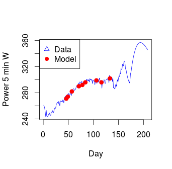
Figure 1: Experimental data (in red) and the solution predicted by the model (in blue)

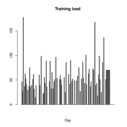
Figure 2: Function $w(t)$

3 Other formulations of the model

In this section, we show other different formulations of the model.

3.1 Problem with three delays

Next, we consider

$$g^{\prime}(t)=-\frac{1}{\tau_{1}}g(t)-\frac{1}{\tau_{2}}g(t-1)-\frac{1}{\tau_{3}}g(t-2)-\frac{1}{\tau_{4}}g(t-3)+w(t).$$ (4)

The solution to (4) can be written as:

$$g(t)=g(0)e^{-\frac{1}{\tau_{1}}t}+\int_{0}^{t}\left[w(s)-\sum_{k=1}^{3}\frac{1}{\tau_{k+1}}g(s-k)\right]e^{-\frac{1}{\tau_{1}}(t-s)}\,ds,\quad t\geq 0,$$

that is,

$$g(t)=\int_{0}^{t}\left[w(s)-\sum_{k=1}^{3}\frac{1}{\tau_{k+1}}g(s-k)\right]e^{-\frac{1}{\tau_{1}}(t-s)}\,ds,\quad t\geq 0,$$

so that,

$$g(n)=\int_{0}^{n}\left[w(s)-\sum_{k=1}^{3}\frac{1}{\tau_{k+1}}g(s-k)\right]e^{-\frac{1}{\tau_{1}}(n-s)}\,ds$$

and we can take, similarly to [14], the approximation

$$g(n)=\sum_{i=0}^{n-1}\left[w(i)-\sum_{k=1}^{3}\frac{1}{\tau_{k+1}}g(i-k)\right]e^{\frac{-1}{\tau_{1}}(n-i)}$$

or

$$g(n)=\sum_{i=0}^{n-1}\left[w(i)-\frac{1}{\tau_{2}}g(i-1)-\frac{1}{\tau_{3}}g(i-2)-\frac{1}{\tau_{4}}g(i-3)\right]e^{\frac{-1}{\tau_{1}}(n-i)}.$$

If we suppose that $w(0)=0$, since $g(s)=0$, $\forall s\in[-3,0]$, we have

$$\begin{split}g(n)&=\sum_{i=1}^{n-1}\left[w(i)-\frac{1}{\tau_{2}}g(i-1)-\frac{1}{\tau_{3}}g(i-2)-\frac{1}{\tau_{4}}g(i-3)\right]e^{\frac{-1}{\tau_{1}}(n-i)}\\ &=\sum_{i=1}^{n-1}w(i)e^{\frac{-1}{\tau_{1}}(n-i)}-\frac{1}{\tau_{2}}\sum_{i=1}^{n-1}g(i-1)e^{\frac{-1}{\tau_{1}}(n-i)}-\frac{1}{\tau_{3}}\sum_{i=1}^{n-1}g(i-2)e^{\frac{-1}{\tau_{1}}(n-i)}\\ &\hskip 30.00005pt-\frac{1}{\tau_{4}}\sum_{i=1}^{n-1}g(i-3)e^{\frac{-1}{\tau_{1}}(n-i)}\\ &=\sum_{i=1}^{n-1}w(i)e^{\frac{-1}{\tau_{1}}(n-i)}-\frac{1}{\tau_{2}}\sum_{i=1}^{n-1}g(i-1)e^{\frac{-1}{\tau_{1}}(n-i)}-\frac{1}{\tau_{3}}\sum_{j=0}^{n-2}g(j-1)e^{\frac{-1}{\tau_{1}}(n-j-1)}\\ &\hskip 30.00005pt-\frac{1}{\tau_{4}}\sum_{j=-1}^{n-3}g(j-1)e^{\frac{-1}{\tau_{1}}(n-j-2)}\\ &=\sum_{i=1}^{n-1}w(i)e^{\frac{-1}{\tau_{1}}(n-i)}-\frac{1}{\tau_{2}}\sum_{i=1}^{n-1}g(i-1)e^{\frac{-1}{\tau_{1}}(n-i)}-\frac{1}{\tau_{3}}\sum_{j=1}^{n-2}g(j-1)e^{\frac{-1}{\tau_{1}}(n-j-1)}\\ &\hskip 30.00005pt-\frac{1}{\tau_{4}}\sum_{j=1}^{n-3}g(j-1)e^{\frac{-1}{\tau_{1}}(n-j-2)}\\ &=\sum_{i=1}^{n-1}w(i)e^{\frac{-1}{\tau_{1}}(n-i)}-\sum_{i=1}^{n-3}g(i-1)\left[\frac{1}{\tau_{2}}e^{\frac{-1}{\tau_{1}}(n-i)}+\frac{1}{\tau_{3}}e^{\frac{-1}{\tau_{1}}(n-i-1)}+\frac{1}{\tau_{4}}e^{\frac{-1}{\tau_{1}}(n-i-2)}\right]\\ &\hskip 30.00005pt-g(n-3)\left[\frac{1}{\tau_{2}}e^{\frac{-2}{\tau_{1}}}+\frac{1}{\tau_{3}}e^{\frac{-1}{\tau_{1}}}\right]-g(n-2)\frac{1}{\tau_{2}}e^{\frac{-1}{\tau_{1}}}\\ &=\sum_{i=1}^{n-1}w(i)e^{\frac{-1}{\tau_{1}}(n-i)}-\sum_{i=1}^{n-3}g(i-1)\left[\frac{1}{\tau_{2}}+\frac{1}{\tau_{3}}e^{\frac{1}{\tau_{1}}}+\frac{1}{\tau_{4}}e^{\frac{2}{\tau_{1}}}\right]e^{\frac{-1}{\tau_{1}}(n-i)}\\ &\hskip 30.00005pt-g(n-3)\left[\frac{1}{\tau_{2}}e^{\frac{-2}{\tau_{1}}}+\frac{1}{\tau_{3}}e^{\frac{-1}{\tau_{1}}}\right]-g(n-2)\frac{1}{\tau_{2}}e^{\frac{-1}{\tau_{1}}}.\end{split}$$

Following for problem (4) a formulation similar to the first one exposed, we have:

$$g(t)=g(k)e^{-\frac{1}{\tau_{1}}(t-k)}+\int_{k}^{t}\left[w(s)-\frac{1}{\tau_{2}}g(s-1)-\frac{1}{\tau_{3}}g(s-2)-\frac{1}{\tau_{4}}g(s-3)\right]e^{-\frac{1}{\tau_{1}}(t-s)}\,ds,$$

for $t\in(k,k+1],$ $k=0,1,\ldots$, so that, we can give the following approximation:

$$\begin{split}g(k+1)&=g(k)e^{-\frac{1}{\tau_{1}}}+\left[w(k)-\frac{1}{\tau_{2}}g(k-1)-\frac{1}{\tau_{3}}g(k-2)-\frac{1}{\tau_{4}}g(k-3)\right]e^{-\frac{1}{\tau_{1}}}\\ &=\left[w(k)+g(k)-\frac{1}{\tau_{2}}g(k-1)-\frac{1}{\tau_{3}}g(k-2)-\frac{1}{\tau_{4}}g(k-3)\right]e^{-\frac{1}{\tau_{1}}},\end{split}$$ (5)

for $k=0,1,\ldots$

3.2 Modelling through an integral equation

We consider

$$g^{\prime}(t)=-\frac{1}{\tau_{1}}g(t)+\tau_{5}\int_{0}^{t}\delta(t,s)g(s)\,ds+w(t).$$ (6)

We can impose, for instance, that $\delta(t,s)=0$ for $s<t-4$. The solution to (6) is obtained as

$$\begin{split}g(t)&=g(0)e^{-\frac{1}{\tau_{1}}t}+\int_{0}^{t}\left[w(u)+\tau_{5}\int_{0}^{u}\delta(u,s)g(s)\,ds\right]e^{-\frac{1}{\tau_{1}}(t-u)}\,du\\ &=\int_{0}^{t}\left[w(u)+\tau_{5}\int_{0}^{u}\delta(u,s)g(s)\,ds\right]e^{-\frac{1}{\tau_{1}}(t-u)}\,du,\quad t\geq 0,\end{split}$$

what gives the approximation

$$\begin{split}g(n)&=\sum_{i=0}^{n-1}\left[w(i)+\tau_{5}\int_{0}^{i}\delta(i,s)g(s)\,ds\right]e^{-\frac{1}{\tau_{1}}(n-i)}\\ &=\sum_{i=0}^{n-1}\left[w(i)+\tau_{5}\sum_{j=0}^{i-1}\delta(i,j)g(j)\right]e^{-\frac{1}{\tau_{1}}(n-i)}.\end{split}$$

From this identity, taking into account that $w(0)=0$ and $g(0)=0$, we get

$$\begin{split}g(n)&=\sum_{i=0}^{n-1}w(i)e^{-\frac{1}{\tau_{1}}(n-i)}+\tau_{5}\sum_{i=0}^{n-1}\sum_{j=0}^{i-1}\delta(i,j)g(j)e^{-\frac{1}{\tau_{1}}(n-i)}\\ &=\sum_{i=1}^{n-1}w(i)e^{-\frac{1}{\tau_{1}}(n-i)}+\tau_{5}\sum_{i=0}^{n-1}\sum_{j=1}^{i-1}\delta(i,j)g(j)e^{-\frac{1}{\tau_{1}}(n-i)}\\ \end{split}$$

If we understand that $\delta(i,j)\neq 0$ only if $j=i-3,i-2,i-1$, we get

$$\begin{split}&\sum_{i=0}^{n-1}\sum_{j=1}^{i-1}\delta(i,j)g(j)e^{-\frac{1}{\tau_{1}}(n-i)}\\ &=\delta(2,1)g(1)e^{-\frac{1}{\tau_{1}}(n-2)}+\sum_{j=1}^{2}\delta(3,j)g(j)e^{-\frac{1}{\tau_{1}}(n-3)}+\sum_{j=1}^{3}\delta(4,j)g(j)e^{-\frac{1}{\tau_{1}}(n-4)}\\ &\hskip 20.00003pt+\sum_{j=1}^{4}\delta(5,j)g(j)e^{-\frac{1}{\tau_{1}}(n-5)}+\cdots+\sum_{j=1}^{n-3}\delta(n-2,j)g(j)e^{-\frac{2}{\tau_{1}}}\\ &\hskip 20.00003pt+\sum_{j=1}^{n-2}\delta(n-1,j)g(j)e^{-\frac{1}{\tau_{1}}}\\ &=\delta(2,1)g(1)e^{-\frac{1}{\tau_{1}}(n-2)}+\sum_{j=1}^{2}\delta(3,j)g(j)e^{-\frac{1}{\tau_{1}}(n-3)}+\sum_{j=1}^{3}\delta(4,j)g(j)e^{-\frac{1}{\tau_{1}}(n-4)}\\ &\hskip 20.00003pt+\sum_{j=2}^{4}\delta(5,j)g(j)e^{-\frac{1}{\tau_{1}}(n-5)}+\cdots+\sum_{j=n-5}^{n-3}\delta(n-2,j)g(j)e^{-\frac{2}{\tau_{1}}}\\ &\hskip 20.00003pt+\sum_{j=n-4}^{n-2}\delta(n-1,j)g(j)e^{-\frac{1}{\tau_{1}}}\\ &=\left[\delta(2,1)e^{-\frac{1}{\tau_{1}}(n-2)}+\delta(3,1)e^{-\frac{1}{\tau_{1}}(n-3)}+\delta(4,1)e^{-\frac{1}{\tau_{1}}(n-4)}\right]g(1)\\ &\hskip 20.00003pt+\left[\delta(3,2)e^{-\frac{1}{\tau_{1}}(n-3)}+\delta(4,2)e^{-\frac{1}{\tau_{1}}(n-4)}+\delta(5,2)e^{-\frac{1}{\tau_{1}}(n-5)}\right]g(2)+\cdots\\ &\hskip 20.00003pt+\left[\delta(n-3,n-4)e^{-\frac{3}{\tau_{1}}}+\delta(n-2,n-4)e^{-\frac{2}{\tau_{1}}}+\delta(n-1,n-4)e^{-\frac{1}{\tau_{1}}}\right]g(n-4)\\ &\hskip 20.00003pt+\left[\delta(n-2,n-3)e^{-\frac{2}{\tau_{1}}}+\delta(n-1,n-3)e^{-\frac{1}{\tau_{1}}}\right]g(n-3)\\ &\hskip 20.00003pt+\delta(n-1,n-2)e^{-\frac{1}{\tau_{1}}}g(n-2)\\ &=\sum_{j=1}^{n-4}\left[\sum_{i=j+1}^{j+3}\delta(i,j)e^{-\frac{1}{\tau_{1}}(n-i)}\right]g(j)+\left[\sum_{i=n-2}^{n-1}\delta(i,n-3)e^{-\frac{1}{\tau_{1}}(n-i)}\right]g(n-3)\\ &\hskip 20.00003pt+\delta(n-1,n-2)e^{-\frac{1}{\tau_{1}}}g(n-2).\end{split}$$

We can proceed by assigning fixed values in $(0,1)$ to

$$\delta(i,i-1),\>\delta(i,i-2),\>\delta(i,i-3),$$

that can be always of the same type, for instance,

$$\delta(i,i-1)=0.5,\>\delta(i,i-2)=0.3,\>\delta(i,i-3)=0.2.$$

Following for problem (6) a formulation similar to the first one exposed, we get:

$$g(t)=g(k)e^{-\frac{1}{\tau_{1}}(t-k)}+\int_{k}^{t}\left[w(u)+\tau_{5}\int_{0}^{u}\delta(u,s)g(s)\,ds\right]e^{-\frac{1}{\tau_{1}}(t-u)}\,du,$$

for $t\in(k,k+1],$ $k=0,1,\ldots$, so that, we can give the approximation:

$$g(k+1)=g(k)e^{-\frac{1}{\tau_{1}}}+\left[w(k)+\tau_{5}\int_{0}^{k}\delta(k,s)g(s)\,ds\right]e^{-\frac{1}{\tau_{1}}}$$

and, taking again an approximation, we get the recursive formula

$$g(k+1)=\left[w(k)+g(k)+\tau_{5}\sum_{j=k-3}^{k-1}\delta(k,j)g(j)\right]e^{-\frac{1}{\tau_{1}}},k=0,1,\ldots$$

If we select always

$$\delta(k,k-1)=0.5,\>\delta(k,k-2)=0.3,\>\delta(k,k-3)=0.2,$$

the recurrence formula is given by:

$$g(k+1)=\left[w(k)+g(k)+0.5\,\tau_{5}\,g(k-1)+0.3\,\tau_{5}\,g(k-2)+0.2\,\tau_{5}\,g(k-3)\right]e^{-\frac{1}{\tau_{1}}},$$ (7)

for $k=0,1,\ldots$, so that, choosing $\delta$ this way, we obtain something similar to the retarded approach, since choosing $\tau_{2}$, $\tau_{3}$ and $\tau_{4}$ such that: $-\frac{1}{\tau_{2}}=0.5\tau_{5}$, $-\frac{1}{\tau_{3}}=0.3\tau_{5}$ and $-\frac{1}{\tau_{4}}=0.2\tau_{5}$, the recurrence formula (7) coincides with (5).

4 Conclusions

In this work, we have shown that, using the model proposed, it is possible to obtain an excellent fit with respect to the experimental data, calculating the positive and negative effects of the training with the ability to predict the effect of training loads in fitness. The improvement of the accuracy in the predicted data leads us definitely to an important tool for planning sports coaching, and new gadgets and software that attempt to control the effect that sports training has on the athlete individually. Besides, this model could be adapted for weight control or to predict the risk of injury or the emotional state of the athlete, issues which play an important role in athletic performance.

We have also provided different models which include several delays or an integro-differential approach.

References

• [1] Banister, E., Calvert, T., Savage, M., and Bach, T. (1975), ‘A systems model of training for athletic performance’, Australian Journal of Sports Medicine 7(3), 57–61.
• [2] Banister, E., Carter, J., and Zarkadas, P. (1999), ‘Training theory and taper: validation in triathlon athletes’, European Journal of Applied Physiology and Occupational Physiology 79(2), 182–191.
• [3] Busso, T. (2003), ‘Variable dose-response relationship between exercise training and performance’, Medicine and Science in Sports and Exercise 35(7), 1188–1195.
• [4] Calvert, T., Banister, E., Savage, M., and Bach, T. (1976), ‘A systems model of the effects of training on physical performance’, IEEE Transactions on Systems, Man and Cybernetics SMC-6(2), 94–102.
• [5] Candau, R., Busso, T., and Lacour, J. (1992), ‘Effects of training on iron status in cross-country skiers’, European Journal of Applied Physiology and Occupational Physiology 64(6), 497–502.
• [6] Clarke, D., and Skiba, P. (2013), ‘Rationale and resources for teaching the mathematical modeling of athletic training and performance’, Advances in Physiology Education 37(2), 134–152.
• [7] Coggan, A. (2006), ‘Training and racing using a power meter: an introduction’.
• [8] Fister, I. Jr., Ljubič, K., Suganthan, P. N., Perc, M., and Fister, I. (2015), ‘Computational intelligence in sports: Challenges and opportunities within a new research domain’, Applied Mathematics and Computation 262, 178–186.
• [9] Fitz-Clarke, J. R., Morton, R. H., and Banister, E. W. (1991) ‘Optimizing athletic performance by influence curves’, Journal of Applied Physiology 71(3), 1151–1158.
• [10] González Badillo, J., and Gorostiaga, E. (1995), Fundamentos del entrenamiento de la fuerza. Aplicación al alto rendimiento deportivo, INDE (in Spanish).
• [11] Hellard, P., Avalos, M., Lacoste, L., Barale, F., Chatard, J.-C., and Millet, G. (2006), ‘Assessing the limitations of the Banister model in monitoring training’, Journal of Sports Sciences 24(5), 509–520.
• [12] Issurin, V. (2010), ‘New horizons for the methodology and physiology of training periodization’, Sports Medicine 40(3), 189–206.
• [13] Morton, R., Fitz-Clarke, J., and Banister, E. (1990), ‘Modeling human performance in running’, Journal of Applied Physiology 69(3), 1171–1177.
• [14] Pfeiffer, M. (2008), ‘Modeling the relationship between training and performance - A Comparison of two antagonistic concepts’, International Journal of Computer Science in Sport, 7(2), 13–32.
• [15] Pfeiffer, M., and Hohmann, A. (2012), ‘Applications of neural networks in training science’, Hum. Mov. Sci. 31(2), 344–359.
• [16] Rodríguez F. A., Iglesias X., Feriche B., Calderón -Soto C., Chaverri D., Wachsmuth N. B., Schmidt W., and Levine B. D. (2015), ‘Altitude Training in Elite Swimmers for Sea Level Performance (Altitude Project)’, Med. Sci. Sports Exerc. 47(9), 1965–1978.