Antiferromagnetic Ising model in an imaginary magnetic field

Abstract

We study the two-dimensional antiferromagnetic Ising model with a purely imaginary magnetic field, which can be thought of as a toy model for the usual $\theta$ physics. Our motivation is to have a benchmark calculation in a system which suffers from a strong sign problem, so that our results can be used to test Monte Carlo methods developed to tackle such problems.

We analyze here this model by means of analytical techniques, computing exactly the first eight cumulants of the expansion of the effective Hamiltonian in powers of the inverse temperature, and calculating physical observables for a large number of degrees of freedom with the help of standard multi-precision algorithms. We report accurate results for the free energy density, internal energy, standard and staggered magnetization, and the position and nature of the critical line, which confirm the mean-field qualitative picture, and which should be quantitatively reliable, at least in the high-temperature regime, including the entire critical line.

I Introduction

One of the major challenges for high-energy and solid-state theorists is the numerical simulation of systems with a severe sign problem. If we denote the microscopic states of a given physical system by $s$, and the thermodynamics of such system is described by a partition function of the form ${\mathcal{Z}}=\sum_{s}P(s)$, we say that the system in question presents a sign problem if the “weights” $P(s)$ are not real and positive: This implies that we cannot interpret $P(s)$ as a proper probability distribution, and the standard, efficient Monte Carlo algorithms cannot be applied. Not all sign problems are equally severe. Let us restrict ourselves for simplicity to the case where the $P(s)$ are real but not positive definite. One can easily devise a reweighting algorithm that uses the absolute value $\left|P(s)\right|$ as the weight of each state, and shifts the sign of $P(s)$ into the observables. Now a standard Monte Carlo method is applicable, and in the limit of infinite statistics we should obtain the correct result. With finite statistics, however, a key quantity is the thermodynamic average of the sign of each contribution to the partition function, that is, $\left<\text{sign}(P(s))\right>$. If this quantity goes to zero exponentially with the volume, $\left<\text{sign}\right>\propto e^{-\alpha V}$, then we would need an exponential amount (in the volume of the system $V$) of statistics to get correct results, which is of course impossible in practice. In this case we say that the sign problem is severe.

QCD at finite baryon density, QCD with a topological term in the action, chains of quantum spins with antiferromagnetic interactions, the two-dimensional O(3) non linear sigma model with a topological term, and the Hubbard model are some of the most popular examples of relevant physical systems where a SSP is present. The existence of a SSP is the main reason for the little progress made on the theoretical understanding of these physical systems outside of phenomenological models.

In order to check novel Monte Carlo methods designed to tackle such problems, it is highly desirable to have a set of benchmark calculations as extensive as possible. For very few systems an analytic solution is known, for example, the one-dimensional antiferromagnetic Ising model with an imaginary magnetic field, the two-dimensional compact U(1) model with topological term, or the two-dimensional Ising model with an imaginary magnetic field $h=i\pi/2$. In a few other cases the sign problem can be avoided by reformulating the physical system with new degrees of freedom, taking advantage of the fact that a good choice of these degrees of freedom provides an equivalent physical system free from the sign problem, which can therefore be simulated by standard methods.

Our motivation for this paper is to provide a benchmark calculation for a system for which we do not have an analytic solution available, nor a reformulation that avoids the sign problem. We study the two-dimensional antiferromagnetic Ising model with a purely imaginary magnetic field, which can be thought of as a toy model for the usual $\theta$ physics. Indeed the Euclidean partition function for QCD with a nonvanishing $\theta$ term can be written in the form

$${\mathcal{Z}}_{V}(\theta)=\sum_{n}p_{V}(n)e^{i\theta n}$$ (1)

where $n$, the topological charge, is an integer, and $p_{V}(n)$ is, up to a normalization, the probability of the topological sector $n$ at $\theta=0$. This has the same structure as the partition function of the antiferromagnetic Ising model in an external purely imaginary magnetic field, as we will see in detail later on, and we expect that the SSP in both systems should also be similar.

This system was studied in Matveev and Shrock (2008) by locating the zeros of the partition function in the complex temperature-magnetic field plane, and they find, for purely imaginary magnetic field, a rich phase structure with two phases characterized by a vanishing (nonvanishing) staggered magnetization, separated by a phase transition line. We study this system by an exact cumulant expansion to eighth order, followed by the analytic computation of the partition function and other physical quantities for a large number of degrees of freedom with the help of a standard multiprecision algorithm. This amounts essentially to the computation of the effective Hamiltonian up to order $T^{-8}$, and therefore is expected to work well in the high-temperature regime, and we provide strong evidence that this is indeed the case. Our results are consistent with Matveev and Shrock (2008), and extend the results of Azcoiti et al. (2011), obtained through the application of algorithms developed in Azcoiti et al. (2002, 2003), and through a mean-field analysis. We are able to obtain a more precise quantitative determination of the transition line separating the paramagnetic and antiferromagnetic phases of the model.

For some systems with a SSP, we know a priori that the partition function will be positive, for example systems in thermal equilibrium with a (Hermitian) Hamiltonian description. Such is the case in a quantum field theory with a $\theta$ term. In the toy model we study here, although we do not have a rigorous proof in this case, we have evidence that, at least in the region where the approximation we use is valid, the partition function is indeed positive (it is trivially always real).

Such evidence is twofold. First, we can prove rigorously that up to the fifth cumulant, the partition function is indeed positive. Unfortunately we have not been able to extend this proof to higher cumulants, but in our multiprecision calculations with up to eight cumulants, we have never seen an instance where the partition function is negative or vanishes. This is highly nontrivial: If instead of a constant imaginary magnetic field we try, for example, to put a staggered imaginary field in our lattice (this is of course equivalent to the ferromagnetic model with a constant imaginary field), we immediately get a fluctuating sign for the partition function.

Second, there have been studies locating the Lee-Yang zeros of the two-dimensional antiferromagnetic Ising model up to $14^{2}$ lattices Kim (2004), and in $12\times 13$ lattices Matveev and Shrock (2008). Up to that size there is no sign of any zeros cutting the imaginary axis at any temperature.

Whereas this by no means amounts to a rigorous proof, we believe it provides a strong indication that, at least in the region of interest for this paper, this model should have a positive partition function.

This paper is organized as follows. Section II is devoted to formulate the model and to recall the main ingredients and results of the mean-field approximation developed in Azcoiti et al. (2011). In Sec. III we introduce the cumulant expansion, report the analytical results for the first eight cumulants in the two-dimensional model, and write the analytical expressions for the free energy and mean values of interesting physical quantities. The results for the staggered magnetization, susceptibility, and phase diagram of the model are reported in Sec. IV, where we also compare our results at $h=0$ and $i\pi/2$ with the analytical solutions of Onsager (1944); Lee and Yang (1952); McCoy and Wu (1967). In Sec. V we report our conclusions. The technical details of the analytical computation of the cumulant expansion can be found in Appendix A, and several tables with numerical results can be found in Appendix B.

II Two-dimensional Ising model

The Ising model Ising (1925); Onsager (1944); Lee and Yang (1952); McCoy and Wu (1967); Matveev and Shrock (1995); McCoy and Wu (1973); Matveev and Shrock (2008) has been studied for a long time now, and it has known analytical solutions in the one-dimensional case at any external magnetic field $h$ Ising (1925), and in two dimensions only for the case without magnetic field $h$ Onsager (1944) and for $h=i\theta/2=i\pi/2$ Lee and Yang (1952); McCoy and Wu (1967). The model with a pure imaginary magnetic field suffers from a SSP in any number of dimensions. In addition to that, the expected phase diagram for $d\geq 2$ is non trivial Azcoiti et al. (2011), making the reconstruction of the $\theta$ dependence of the observables even more challenging. All this makes the model a good theoretical laboratory to test new methods designed to deal with the SSP. It is therefore worthwhile to carry out a detailed study of this model at purely imaginary magnetic field, particularly because little progress has been achieved on reconstructing the $\theta$ dependence of the observables, apart from the analysis of Azcoiti et al. (2011) and the recent study in de Forcrand and Rindlisbacher (2016).

The partition function of the model, following the conventions of Azcoiti et al. (2011), is:

$${\mathcal{Z}}=\sum_{\{s_{i}\}}\exp{\left(F\sum_{<ij>}{s_{i}s_{j}}+i\theta\dfrac{1}{2}\sum_{i}{s_{i}}\right)}.$$ (2)

The half magnetization

$$\dfrac{M}{2}\equiv\dfrac{1}{2}\sum_{i}s_{i},$$ (3)

is an integer taking any value between $-N/2$ and $N/2$, where $N$ is an even number denoting the total number of spins in the lattice. It is in this sense that we identify $M/2$ with a topological charge and regard the imaginary magnetic field term in the action as a $\theta$ term. It is important to mention that, from now on, we will consider only the antiferromagnetic case $F<0$, since the model with imaginary field does not define a unitary theory for arbitrary values of the ferromagnetic coupling Lee and Yang (1952); Azcoiti and Galante (1999).

As we shall see in detail in the next section, by dividing the rectangular lattice into two sublattices, introducing the respective magnetizations $M_{1}$ and $M_{2}$, making a cumulant expansion and keeping only the first cumulant, we arrive at the following approximation to the partition function (where $d$ denotes the dimensionality of the lattice):

$${\mathcal{Z}}_{1c}(F,\theta)=\sum_{\{s_{i}\}}\exp\left(i\theta\dfrac{M_{1}+M_{2}}{2}+4\dfrac{Fd}{N}M_{1}M_{2}\right).$$ (4)

We recall now the mean-field analysis carried out in Azcoiti et al. (2011). The resulting partition function,

$${\mathcal{Z}}_{MF}(F,\theta)=\sum_{\{s_{i}\}}\exp\left(i\theta\dfrac{M_{1}+M_{2}}{2}-\dfrac{Fd}{N}(M_{1}-M_{2})^{2}\right),$$ (5)

is different from Eq. (4). However, it can be seen to give the same qualitative results for the observables and the phase diagram. In this regard, we will consider the first-cumulant expansion ${\mathcal{Z}}_{1c}$ as a mean-field approximation to ${\mathcal{Z}}$, and the general expansion itself as an improvement of it, at least for small $F$, where the expansion is expected to converge.

Applying standard saddle-point techniques to the mean-field partition function Azcoiti et al. (2011), one obtains the $F-\theta$ phase diagram shown in Fig. 1. A second order critical line,

$$dF_{c}=\dfrac{1}{2}\cos^{2}{\dfrac{\theta_{c}}{2}},$$ (6)

separates two different phases: a staggered one, with $\langle m_{s}\rangle\neq 0$, for $\theta\geq\theta_{c}$, and a paramagnetic one, with $\langle m_{s}\rangle=0$, for $\theta<\theta_{c}$.

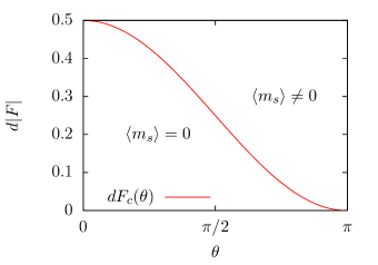
Figure 1: Phase diagram of the mean-field approach of Azcoiti et al. (2011) to the antiferromagnetic Ising model in the $F-\theta$ plane.

III Cumulant expansion and observables

Our interest is focused on the antiferromagnetic model, where the staggered magnetization is a good order parameter. From now on we will work with a rectangular two-dimensional lattice, although the method is easily generalizable to any number of dimensions. We divide the lattice into two sublattices $\Omega_{1}$ and $\Omega_{2}$ in a chessboard fashion. In the two-dimensional lattice this means that if $i$ and $j$ index, respectively, the row and the column of a given spin, this spin will be in the first (second) sublattice if the sum $i+j$ is even (odd). For simplicity we will require that both lengths of the lattice be even. Denoting by $N$ the total number of points in the lattice, we define the magnetization densities $m_{1}$ and $m_{2}$ as

$$m_{j}\equiv\dfrac{M_{j}}{N/2}\equiv\dfrac{\sum_{i\in\Omega_{j}}s_{i}}{N/2}\qquad j=1,2,$$ (7)

and the density of staggered magnetization is

$$m_{s}\equiv\dfrac{m_{1}-m_{2}}{2}.$$ (8)

Let us denote by $g(m_{1},m_{2})$ the number of microstates with magnetization densities $m_{1}$ and $m_{2}$ in sublattices $\Omega_{1}$ and $\Omega_{2}$, respectively, that is,

$$g(m_{1},m_{2})=\sum_{\{s_{i}\}}\delta\left(\sum_{i\in\Omega_{1}}s_{i}-M_{1}\right)\delta\left(\sum_{i\in\Omega_{2}}s_{i}-M_{2}\right).$$ (9)

A trivial computation gives:

$$g(m_{1},m_{2})=\binom{N/2}{N_{1+}}\binom{N/2}{N_{2+}},$$ (10)

with $N_{j+}\equiv N(1+m_{j})/4$ for $j=1,2$. Defining now the expected value at fixed $m1,m2$ as:

$$\left<\mathcal{O}\right>_{m_{1},m_{2}} \equiv \frac{1}{g(m_{1},m_{2})}$$

$$\times\sum_{\{s_{i}\}}\delta(\sum_{i\in\Omega_{1}}s_{i}-M_{1})\delta(\sum_{i\in\Omega_{2}}s_{i}-M_{2})\;\mathcal{O}$$

we can rewrite the partition function (2) in the form:

$${\mathcal{Z}} = \sum_{m_{1},m_{2}}g(m_{1},m_{2})$$ (12)

$$\times\left<\exp{\left(i\frac{\theta}{2}\sum_{i}s_{i}+F\sum_{<ij>}{s_{i}s_{j}}\right)}\right>_{m_{1},m_{2}}.$$

The $\theta$ term in Eq. (12) is just $i\theta\left(m_{1}+m_{2}\right)N/4$, and therefore constant under fixed $m_{1}$ and $m_{2}$; we can take it out of the expected value, arriving at

$${\mathcal{Z}} = \sum_{m_{1},m_{2}}g(m_{1},m_{2})e^{\frac{1}{4}Ni\theta(m_{1}+m_{2})}$$ (13)

$$\times\left<\exp{\left(F\sum_{<ij>}{s_{i}s_{j}}\right)}\right>_{m_{1},m_{2}}.$$

We cannot evaluate exactly the expectation value in Eq. (13), as that would be equivalent to solving exactly the model for arbitrary values of the external field. Instead we perform a cumulant expansion and truncate at a given order. Let us recall the definition:

$$\left<e^{tX}\right>\equiv\exp{\left(\sum_{n=1}^{\infty}\kappa_{n}\dfrac{t^{n}}{n!}\right)},$$ (14)

where the $n$th cumulant $\kappa_{n}$ is an $n$th degree polynomial in the first $n$ noncentral moments of $X$, given by the following recursion formula:

$$\kappa_{n}=\mu^{\prime}_{n}-\sum_{m=1}^{n-1}\binom{n-1}{m-1}\kappa_{m}\mu^{\prime}_{n-m},\qquad\mu^{\prime}_{n}\equiv\left<X^{n}\right>.$$ (15)

By expanding in cumulants in our partition function, taking $t=F$ and $X=\sum s_{i}s_{j}$, we obtain

$${\mathcal{Z}} = \sum_{m_{1},m_{2}}g(m_{1},m_{2})$$

$$\times\exp{\left(\frac{1}{4}Ni\theta(m_{1}+m_{2})+\sum_{n=1}^{\infty}\kappa_{n}(m_{1},m_{2})\dfrac{F^{n}}{n!}\right)},$$

where now the moments are given by

$$\mu^{\prime}_{n}=\left<\left(\sum_{<i,j>}s_{i}s_{j}\right)^{n}\right>_{m_{1},m_{2}}.$$ (17)

The computation of these quantities is somewhat involved, and we relegate the details to Appendix A. We calculate the cumulants using a numerical (but exact) method, up to $n=8$. The results, at leading order in $N$, for $d=2$, are

$$\kappa_{1} = 2Nm_{1}m_{2},$$

$$\kappa_{2} = 2N({m_{1}}^{2}-1)({m_{2}}^{2}-1),$$

$$\kappa_{3} = 8Nm_{1}m_{2}({m_{1}}^{2}-1)({m_{2}}^{2}-1),$$

$$\kappa_{4} = 4N(21{m_{1}}^{2}{m_{2}}^{2}-9({m_{1}}^{2}+{m_{2}}^{2})+5)$$

$$\times({m_{1}}^{2}-1)({m_{2}}^{2}-1),$$

$$\kappa_{5} = 32N(51{m_{1}}^{2}{m_{2}}^{2}-39{m_{1}}^{2}-39{m_{2}}^{2}+31)$$

$$\times m_{1}m_{2}({m_{1}}^{2}-1)({m_{2}}^{2}-1),$$

$$\kappa_{6} = 64N(675{m_{1}}^{4}{m_{2}}^{4}-690[{m_{1}}^{4}{m_{2}}^{2}+{m_{1}}^{2}{m_{2}}^{4}]$$

$$+705{m_{1}}^{2}{m_{2}}^{2}+75[{m_{1}}^{4}+{m_{2}}^{4}-{m_{1}}^{2}-{m_{2}}^{2}]+8)$$

$$\times({m_{1}}^{2}-1)({m_{2}}^{2}-1),$$

$$\kappa_{7} = 128N(10935m_{1}^{4}m_{2}^{4}-13950[m_{1}^{4}m_{2}^{2}+m_{1}^{2}m_{2}^{4}]$$

$$+3375[m_{1}^{4}+m_{2}^{4}]+17760m_{1}^{2}m_{2}^{2}-4290[m_{1}^{2}+m_{2}^{2}]$$

$$+1051)m_{1}m_{2}(m_{1}^{2}-1)(m_{2}^{2}-1).$$

$$\kappa_{8} = 32N(1685565{m_{1}}^{6}{m_{2}}^{6}-2604735[{m_{1}}^{6}{m_{2}}^{4}$$ (18)

$$+{m_{1}}^{4}{m_{2}}^{6}]+994455[{m_{1}}^{6}{m_{2}}^{2}+{m_{1}}^{2}{m_{2}}^{6}]$$

$$-55125[{m_{1}}^{6}+{m_{2}}^{6}]+4026645{m_{1}}^{4}{m_{2}}^{4}$$

$$-1541085[{m_{1}}^{4}{m_{2}}^{2}+{m_{1}}^{2}{m_{2}}^{4}]+85575[{m_{1}}^{4}+{m_{2}}^{4}]$$

$$+595077{m_{1}}^{2}{m_{2}}^{2}-33663[{m_{1}}^{2}+{m_{2}}^{2}]+2125)$$

$$\times(m_{1}^{2}-1)(m_{2}^{2}-1)$$

Now we can compute an approximation to the expected value of any observable of the form $\mathcal{O}(m_{1},m_{2})$ as follows:

$$\left<\mathcal{O}\right> = \dfrac{1}{{\mathcal{Z}}}\sum_{m_{1},m_{2}}\mathcal{O}(m_{1},m_{2})g(m_{1},m_{2})$$

$$\times\exp\left\{i\theta\dfrac{M_{1}+M_{2}}{2}+\sum_{n=1}^{n_{max}}\dfrac{F^{n}}{n!}\kappa_{n}(m_{1},m_{2})\right\},$$

where $\left<\mathcal{O}\right>$ depends implicitly on the number of cumulants included in the approximation, $n_{max}$, and on the number of spins of the system $N$. Taking the limit of both $n_{max}$ and $N$ to infinity, we should recover the exact result in the thermodynamic limit. Using this technique, we have computed several observables, such as the density of free energy $\phi$, the density of internal energy $e$, the specific heat $c_{v}$ and both the usual and the staggered magnetization $\langle m\rangle$ and $\langle m_{s}\rangle$, respectively. The precise definitions of the computed observables are the following:

$$\phi \equiv -\dfrac{1}{NF}\log{\mathcal{Z}},$$ (20)

$$e \equiv -\dfrac{1}{2N}\dfrac{d\log{\mathcal{Z}}}{dF},\qquad c_{v}\equiv-F^{2}\dfrac{d}{dF}e,$$ (21)

$$\langle m\rangle \equiv \left<\dfrac{m_{1}+m_{2}}{2}\right>,\qquad\langle m_{s}\rangle\equiv\left<\dfrac{m_{1}-m_{2}}{2}\right>.$$ (22)

It must be noted that at $\theta=\pi$, where the model has an analytical solution, the free energy has a singularity at $F=0$ Lee and Yang (1952); McCoy and Wu (1967). In the next section we will talk about its nonsingular part, which is simply the result of subtracting the singular term from the full expression:

$$\phi\equiv\phi_{ns}-\dfrac{1}{2F}\log{(1-e^{4F})}.$$ (23)

As we have mentioned before, the complex-valued exponentials in Eq. (LABEL:sumExponentials) give rise to a severe sign problem. To deal with it we use a multiprecision algorithm, which allows us to keep as many digits as needed. In order to crosscheck our calculations we have used several multiprecision libraries (GMP, GNU MPFR, GNU MPC, gmpy2) to do the sum over $m_{1}$ and $m_{2}$. The computational cost when computing the observables grows on one hand with $N^{2}$ due to the number of summands in (LABEL:sumExponentials). In addition to that, the number of digits needed grows linearly with $N$, increasing the cost of each multiprecision operation.

IV Results

At $\theta=0$ and $\pi$ we know the analytical solution for the two-dimensional Ising model Onsager (1944); Lee and Yang (1952); McCoy and Wu (1967), and therefore we can compare the exact results with the approximations obtained from Eq. (LABEL:sumExponentials). We can see in Figs. 2 and 3 the density of free energy as a function of the coupling $|F|$, for different approximations. Concretely we show the approximations obtained by keeping only the first, up to the fourth, and up to the eighth cumulant. For clarity we show only the results corresponding to the largest size $N$ that we have calculated, although we have carefully checked that the finite-size effects are tiny at that value of $N$. We can see that the agreement with the exact result, especially for the fourth and eighth approximations, is excellent at small $|F|$, where we can expect the cumulant expansion to be well behaved. At $|F|\gtrsim 0.57$ the approximations start to drift away from the analytic result, especially the eighth, possibly indicating the lack of convergence of the cumulant expansion at such larger couplings.

The above results are consistent with those of the density of internal energy, which we can see in Figs. 4-6. The same can be said about the specific heat for $\theta=\pi$, in Fig. 7. The results of the specific heat for $\theta=0$, in Fig. 8, show also a good agreement with the analytical solution, as long as we are far from the critical point. In the neighborhood of the critical point we can see that keeping a finite number of cumulants has a strong impact. However, the results seem to converge to the exact solution quickly when we increase the number of cumulants, and indeed the peak when including all eight cumulants is not far from the analytic result.

The agreement with the exact results both at $\theta=0$ and at $\pi$ suggests that the cumulant expansion can be trusted at all values of $\theta$, as long as $|F|\lesssim 0.57$.

We expect a nonvanishing value of $\langle m_{s}\rangle$ to signal the transition from the paramagnetic to the staggered phase. Because of translational symmetry, we cannot simply compute this observable, since for a finite $N$ system it is always zero [permuting $m_{1}$ and $m_{2}$ leaves Eq. (LABEL:sumExponentials) invariant]. However, we can compute $\langle m_{s}^{2}\rangle$, which also separates the weak and strong coupling phases.

In Fig. 9 we show results for $\langle m_{s}^{2}\rangle$ at $\theta=2$. One can see how, as we approach the thermodynamic limit, $\langle m_{s}^{2}\rangle$ becomes a steeper function of $|F|$. To obtain the critical line for a given cumulant approximation, we numerically calculate the quantity $\frac{d}{d\theta}\langle m_{s}^{2}\rangle$ (which should diverge in the thermodynamic limit at the critical line), and find the maximum along lines of constant $\theta$. This gives us, for each size $N$ and each value of $\theta$, $F_{c}(\theta)$. We can see in Fig. 10 the behavior of such quantity as a function of $F$ and $N$, for the specific value $\theta=2$, in the eight cumulant approximation. The height of the peak does not scale as $N$, at least at the volumes we have been able to calculate, therefore suggesting a continuous phase transition; however, our data are not extensive enough to calculate the critical exponents.

The phase diagram obtained in this way is shown in Fig. 11, for several truncation orders of the cumulant expansion. The transition lines that we obtain lie entirely below $|F|=.45$, where we have good evidence that the cumulant expansion works well. The change from the line corresponding to $k=1$ and $4$ is very large, but the results seem to stabilize quickly with the order of the expansion, and the lines corresponding to $k=4$ and $8$ are quite close together. Therefore we expect the phase diagram for $k=8$ to be a quite accurate approximation to the exact one. Further evidence of this is the agreement with the few maximal values for $F_{c}$ estimated in Matveev and Shrock (2008) from the computation of the zeros of the partition function of the model in the complex temperature-magnetic field plane. As can be seen in the plot, they lie above but quite close to our $k=8$ line.

As another crosscheck we show in Fig. 12 results for the specific heat at $\theta=2$ in the eight cumulant approximation, computed for several system sizes. The behavior is similar to the one in Fig. 10: a peak of increasing height in the vicinity of the critical point, and smooth behavior and small finite N effects elsewhere.

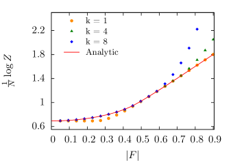
Figure 2: Free energy ($-F\phi$) at $\theta=0,N=2000$ for the square-lattice AF Ising model in the $k$th cumulant approximation.

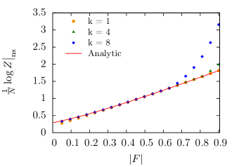
Figure 3: Nonsingular part of the free energy ($-F\phi$) at $\theta=\pi,N=2000$.

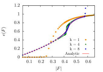
Figure 4: Internal energy $e(F)$ computed for one, four, and eight cumulants at $\theta=0$ and $N=2000$.

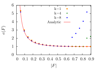
Figure 5: Internal energy density $e(F)$ at $\theta=\pi,N=2000$ at several cumulant expansions.

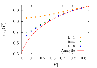
Figure 6: nonsingular part of the internal energy at $\theta=\pi,N=2000$.

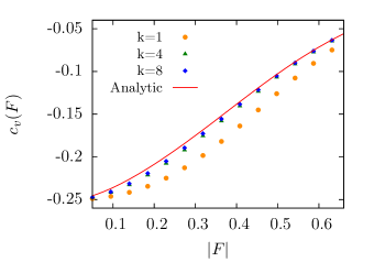
Figure 7: Specific heat at $\theta=\pi,N=2000$, plotted against the analytical expression.

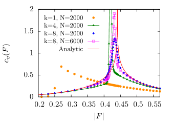
Figure 8: Specific heat at $\theta=0$, plotted against the analytical solution. At $\theta=0$, $F_{c}=\log(1+\sqrt{2})/2\approx 0.4407$.

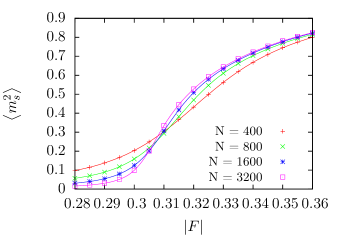
Figure 9: $\langle m_{s}^{2}\rangle$ curves at $\theta=2,k=8$. Solid lines are just a guide to the eye.

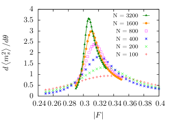
Figure 10: Scaling of $d\langle m_{s}^{2}\rangle/d\theta$ at $\theta=2,k=8$. Solid lines are a guide to the eye.

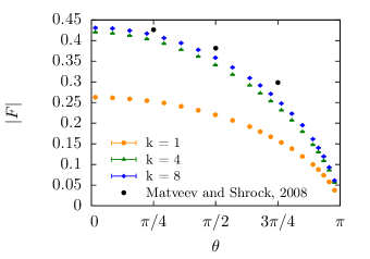
Figure 11: The critical line $F_{c}(\theta)$, computed as the maximum of $d\langle m_{s}^{2}\rangle/d\theta$ at $N=2000$. The maximal $F$ points obtained in Matveev and Shrock (2008) are also shown.

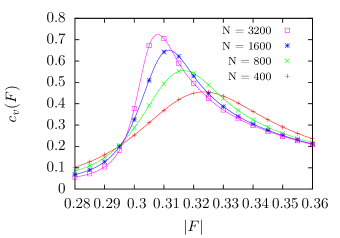
Figure 12: Specific heat $c_{v}$ with $k=8$ and $\theta=2$. Solid lines are just a guide to the eye.

V Conclusions

We have analyzed the two-dimensional antiferromagnetic Ising model with an imaginary magnetic field by analytical techniques. We have calculated the first eight cumulants of what is essentially the expansion of the effective Hamiltonian in powers of the inverse temperature, and computed physical quantities for a large number of degrees of freedom with the help of multiprecision algorithms. The motivation for such a calculation was to have an example of a physical system with SSP and nontrivial phase structure, the dynamics of which is well known, at least in the high-temperature region.

Our results confirm the qualitative picture described in Azcoiti et al. (2011), and predict the existence of two phases in this model, which can be characterized by the staggered magnetization as an order parameter. The finite-size scaling suggests that the two phases are separated by a continuous phase transition line. The position of the critical point at $\theta=0$ is in very good agreement with the exact result $F_{c}=\log(1+\sqrt{2})/2\approx 0.4407$, and the free and internal energy densities at $\theta=\pi$ agree also well with the analytical prediction, at least in the high-temperature regime, thus giving reliability to our results in this region. Therefore this model could be a good laboratory to check proposals to simulate physical systems afflicted by a SSP.

Appendix A Computation of the cumulants $\kappa_{n}$

In order to use expressions (LABEL:ZenKappas) and (LABEL:sumExponentials), we need to compute the cumulants $\kappa_{n}$. The $n$th cumulant can be calculated in terms of the first $n$ noncentral moments $\mu^{\prime}_{n}$,

$$\mu^{\prime}_{n}\equiv\left<\left(\sum_{<ij>}s_{i}s_{j}\right)^{n}\right>_{m_{1},m_{2}},$$ (24)

by means of the recursion relation (15). The summation over $<ij>$ runs over each couple of neighboring spins, or in other words, over each link. Two neighboring spins always belong to different sublattices.

Before going further, let us comment on two intermediate results. First, we consider a lattice of $N$ spins, the magnetization of which is the sum $m=\sum_{i}s_{i}$, and ask about the expected value of the product of $n$ of these spins at fixed $m$ (or fixed $N_{+}$, the number of positive spins), that is, $\langle s_{1}s_{2}\cdots s_{n}\rangle_{m}$. One can perform this calculation by means of the microcanonical formalism, arriving at

$$\langle s_{1}s_{2}\cdots s_{n}\rangle_{m}=\dfrac{1}{\binom{N}{N_{+}}}\sum_{k=0}^{n}(-1)^{k}\binom{n}{k}\binom{N-n}{N_{+}-n+k}.$$ (25)

In the above expression, $k$ can be read as the number of negative spins in the product $s_{1}s_{2}\cdots s_{n}$. In this way, the first summand, $k=0$, counts the number of states with zero negative spins in the product $s_{1}s_{2}\cdots s_{n}$ and multiplies it by the expected value of the product in this case, $(-1)^{0}=1$. The second one, $k=1$, does the same for one negative spin in $s_{1}\cdots s_{n}$, and so on. Dividing the sum by the total number of configurations with magnetization $m=2N_{+}/N-1$, one obtains the previous expected value at fixed $m$. Secondly, consider an observable $\mathcal{O}(m_{1},m_{2})$ in our two sublattice system, with a dependence on $m_{1}$ and $m_{2}$ such as we can write it as $\mathcal{O}_{1}(m_{1})\mathcal{O}_{2}(m_{2})$. In this case, from the definition (LABEL:defmicro) of the expected value at fixed $m_{1}$ and $m_{2}$, we have

$$\left<\mathcal{O}_{1}(m_{1})\mathcal{O}_{2}(m_{2})\right>_{m_{1},m_{2}}=\left<\mathcal{O}_{1}(m_{1})\right>_{m_{1}}\left<\mathcal{O}_{2}(m_{2})\right>_{m_{2}}.$$ (26)

This immediately applies to the spin product $s_{1}s_{2}\cdots s_{n}$. We can always divide it into two products $s_{a}\cdots s_{b}$ and $s_{\alpha}\cdots s_{\beta}$, each one containing the spins of one of the sublattices, and then

$$\left<s_{1}s_{2}\cdots s_{n}\right>_{m_{1},m_{2}}=\left<s_{a}\cdots s_{b}\right>_{m_{1}}\left<s_{\alpha}\cdots s_{\beta}\right>_{m_{2}}.$$ (27)

With the previous couple of results, we come back to Eq. (24), and apply the linearity of the expected value, arriving at

$$\mu^{\prime}_{n}=\sum_{<ij>,<kl>,\cdots,<pq>}\left<s_{i}s_{j}s_{k}s_{l}\cdots s_{p}s_{q}\right>_{m_{1},m_{2}},$$ (28)

which is the sum of the expected values of the product of $n$ links, running over all permutations with repetitions of these links. Then, in every summand we have the product of $2n$ spins, in some cases with some of them identical. Taking into account that $s_{i}^{2}=1\>\forall i$, each summand can be reduced to the expected value of the product of $n_{1}+n_{2}$ different spins, $n_{1}$ and $n_{2}$ being the number of spins in each sublattice. Since by means of Eq. (25) we already have an expression that computes $\langle s_{1}\cdots s_{n}\rangle_{m}$, the problem is reduced to count how many summands in Eq. (28) have $(n_{1},n_{2})$ spins. We call these numbers geometrical factors, and denote them by $\mathcal{G}(n_{1},n_{2})$. Following this convention, we can write the $n$th central moment as

$$\mu^{\prime}_{n}=\sum_{\{n_{1},n_{2}\}}\mathcal{G}(n_{1},n_{2})\langle\underbrace{s_{a}\cdots s_{b}}_{n_{1}\>\text{spins}}\rangle_{m_{1}}\langle\underbrace{s_{\alpha}\cdots s_{\beta}}_{n_{2}\>\text{spins}}\rangle_{m_{2}},$$ (29)

where the sum runs over the couples of integers $(n_{1},n_{2})$ the sum of which is even and less than or equal to $n$.

The computation of the geometrical factors $\mathcal{G}(n_{1},n_{2})$ can be done by hand for the first few cumulants. As an example, for the second noncentral moment $\mu^{\prime}_{2}$ we have to compute four cases: the two links being the same (sharing both spins), sharing only one spin belonging to the first or the second sublattice, and finally not sharing any spin at all. That is, in terms of the previous notation,

$$\{(n_{1},n_{2})\}=\{(0,0),(2,0),(0,2),(2,2)\}.$$ (30)

The factors $\mathcal{G}(n_{1},n_{2})$ can be computed easily in this case, even for an hypercubic lattice of arbitrary dimension $d$, arriving at the following expression for the second moment

$$\mu^{\prime}_{2} = Nd\langle 1\rangle+Nd(d-1)(\langle s_{1}s_{2}\rangle_{m_{1}}+\langle s_{1}s_{2}\rangle_{m_{2}})$$

$$+Nd(Nd-2(d-1)-1)\langle s_{1}s_{2}\rangle_{m_{1}}\langle s_{1}s_{2}\rangle_{m_{2}}.$$

We can use this expression to calculate the second cumulant $\kappa_{2}$,

$$\kappa_{2}=\mu^{\prime}_{2}-{\mu^{\prime}}_{1}^{2}\xrightarrow{N\to\infty}Nd(m_{1}^{2}-1)(m_{2}^{2}-1),$$ (32)

where we have taken the thermodynamic limit, keeping only the terms of order $\mathcal{O}(N)$, which is the leading order for all cumulants. Subleading orders can be preserved if needed, but they are not relevant for our paper. The difficulty of the previous computation escalates quickly with the order $n$ of the cumulant, and it is quite cumbersome for just $n\geq 4$. In order to get beyond this limitation, we have developed a program which computes the geometrical factors $\mathcal{G}(n_{1},n_{2})$ numerically for a finite $L\times L$ bidimensional lattice. Since these factors $\mathcal{G}(n_{1},n_{2})$ are polynomials in $N$ of order $\leq n$ (and with integer coefficients), we can run the program for lattices of $n+1$ different sizes, obtaining a set of ($N$,$\mathcal{G}(N)$) points, which we can use to recover the exact integer coefficients of each geometrical factor, by means of the Lagrange interpolation formula.

The basic idea of the program is very simple. We just construct a periodic rectangular $L\times M$ lattice, with $L,M>n$, $n$ being the order of the cumulant we want to compute. With this restriction we avoid products of links crossing the entire lattice, that would not appear in the thermodynamic limit for any finite cumulant. Once we have this, we start a loop running over all the permutations with repetitions of $n$ links, and perform the following steps,

• We have a product of $n$ links, or equivalently $2n$ spins, $s_{1}\cdots s_{2n}$.

• Recursively, we remove couples of equal spins from this product.

• We classify the remaining product by the number of spins in each sublattice, $(n_{1},n_{2})$.

• We add one to the geometric factor $\mathcal{G}(n_{1},n_{2})$ and proceed to the next iteration.

When the algorithm finishes, we obtain all the $\mathcal{G}(n_{1},n_{2})$ values for a given $N=LM$. The computational cost is associated to the number of iterations of the main loop, which grows as ${(LM)}^{n}$, that is, exponentially with the order of the cumulant. In practice, we have only reached the computation of the fourth cumulant with this program. However, a number of optimizations can be implemented in order to reach higher order cumulants, which we summarize in what follows.

A.1 Translational symmetry

Our lattice is symmetric under translations, implying that all geometrical factors are proportional to $Nd$, the number of links. Fixing, e.g., the first link of the product, one obtains the same $\mathcal{G}(n_{1},n_{2})$, but divided by a common factor $Nd$. The same factor is gained in the overall speed of the program. In addition to that, the degree of the polynomials $\mathcal{G}(n_{1},n_{2})$ is also reduced by one, and it suffices with $n$ (instead of $n+1$) different sizes in order to recover the $N$ dependence. One can go even further by realizing that the geometrical factor corresponding to non-neighboring links, $\mathcal{G}(n,n)$, is the only one with maximum degree $N^{n-1}$. This allows us to express it in terms of the remaining factors,

$$\dfrac{1}{Nd}\mathcal{G}(n,n) = (Nd)^{n-1}$$ (33)

$$-\dfrac{1}{Nd}\sum_{\{(n_{1},n_{2})\}\backslash(n,n)}\mathcal{G}(n_{1},n_{2}),$$

which are only of order $n-2$ or less. This means that it is enough to run the program for $n-1$ lattice sizes, compute all the geometrical factors but $\mathcal{G}(n,n)$ via the Lagrange interpolator, and then with the previous expression find the $N$ dependence of this last factor.

A.2 From permutations to combinations

The product of links commutes, so its contribution to the geometrical factors is the same regardless of the order. Then, we can change the main loop over permutations with repetition to a loop over combinations with repetition, by taking into account the multiplicity of each combination. Schematically, we perform

$$\sum_{i,j,\dots,k} \text{contrib}(l_{i}l_{j}\cdots l_{k})$$ (34)

$$\rightarrow\sum_{i\leq j\leq\cdots\leq k}\text{mult}\times\text{contrib}(l_{i}l_{j}\cdots l_{k}),$$

where contrib represents a function in our program that takes a product of links and returns the contribution to the geometrical factors. If there are $r$ different links, each one appearing $k_{1},\dots,k_{r}$ times, the multiplicity of the combination is given by

$$\text{mult}=\dfrac{n!}{k_{1}!\cdots k_{r}!}.$$ (35)

A.3 Blocks - Grouping links together

Many of the link products have few, if any, repeated spins, and their contributions to the geometrical factors can be counted without having to analyze one by one each of them. This is possible by grouping them in sets of links that we will call in what follows blocks, and replacing the loop over link products by a loop over block products. When the blocks in a product are not neighbors (i.e., they do not have any common spin), we do not need to perform the computation link by link and the contribution can be summed up trivially. Let $b_{1}$ and $b_{3}$ be two non-neighboring blocks, each one composed by $N_{b}$ links, and let us denote the contributions to the geometrical factors by $\lambda(n_{1},n_{2})$, where $\lambda$ is an integer counting how many products of links have $n_{1}$ ($n_{2}$) spins in the first (second) sublattice. Then we have

$$contrib(b_{1}b_{3})=N_{b}^{2}(2,2),$$ (36)

or in general, for the product of $k$ non-neighboring blocks, $N_{b}^{k}(k,k)$. Following this strategy, we divide our lattice into unidimensional blocks of $2M$ links, in a way that the $j$th block, $b_{j}$, contains all links the first spin of which belongs to the $j$th column. As a consequence, $b_{j}$ is a neighbor of blocks $j-1$ and $j+1$, and, taking into account the boundary conditions, $b_{0}$ and $b_{L-1}$ are neighbors too.

When we have a product of neighboring blocks, we proceed as before, analyzing the link products one by one, and there is no computational saving. But when the $n$ blocks are not neighbors, we move from $(Nd)^{n}$ iterations to a single one.

A.4 Clusters of blocks

The block method, as defined above, fails to save any computation time if two or more blocks are neighbors in a given block product. However, we can extend the method by dividing each block product into several subproducts, which we will denote as clusters. In each cluster, one can always connect one block to another by the equivalence relation of being neighbors (sharing spins). And in the same way, in each product different clusters never share any spin. This allows us to compute the contributions of each cluster separately, and then compose them with the following law,

$$\lambda_{1}(a,b)\oplus\lambda_{2}(c,d)=\lambda_{1}\lambda_{2}(a+c,b+d).$$ (37)

If the contributions of the clusters involve more than one geometrical factor, linearity applies,

$$\sum_{ab}\lambda_{ab}(a,b) \oplus \sum_{cd}\lambda_{cd}(c,d)=$$ (38)

$$\sum_{ab,cd}\lambda_{ab}\lambda_{cd}(a+c,b+d).$$

Processing one cluster with $k$ blocks takes a computing time proportional to $(Nd)^{k}$. So dividing the whole block product in smaller clusters implies for almost every block product a significant amount of time saved. Only when all the blocks are part of the same cluster there is no speed up.

Another major optimization can be performed by realizing that translational invariance can also be applied here, since a given cluster, say $b_{0}b_{1}b_{1}$, and any of its translations, $b_{0+t}b_{1+t}b_{1+t}$, have the same contribution to the geometrical factors. Then, when a cluster is going to be computed, we can express it in terms of its equivalence class, compute its contribution, and store it in memory. Every time one of its translations appears, we just take the value from the memory, saving a lot of computing time. In addition to that, once we have computed the factors $\mathcal{G}(n_{1},n_{2})$ for the first size $L\times M$, we know in advance all the cluster contributions for any $L^{\prime}\times M$ lattice (the blocks keep its size constant). Since almost all the computing time is spent in figuring out the cluster contributions, we reduce in this way the full problem of computing the geometrical factors in lattices of $n-1$ different sizes to only one size, the smallest one, $M\times M$. In practice, the time spent by the rest of the sizes needed is barely the $1-2\%$ of that of the first size.

A.5 Computation of a cluster

The last optimization concerns the computation of the clusters themselves. Until now it is done simply by performing a loop over each possible permutation of links belonging to each of the blocks in the cluster. However, one can go one step further and divide the blocks composing the cluster into smaller sets, that we will call sites. A site is simply the set of two links the first spin of which lies in the site $i,j$, that is,

$$\text{site}(i,j)\equiv\{s_{ij}s_{i+1,j},s_{ij}s_{i,j+1}\}.$$ (39)

With this new subdivision, we can apply in the same way the techniques described above. In order to compute the cluster $b_{1}\dots b_{k}$, we start a loop over every permutation of sites $s_{1}\dots s_{k}$, with $s_{i}\in b_{i}$. Each site product is divided into clusters, the contributions of which can be summed with Eq. (38) and are calculated by performing another loop over each link product ($2^{k}$ iterations for a site product of $k$ elements). Finally, by summing up each site product contribution, we obtain the whole cluster contribution.

All the described optimizations do not remove the exponential dependence on $n$ of the algorithm. However, they allow us to reach the eighth cumulant, which takes about three days of computing time in a modern laptop.

Appendix B Numerical tables

In this appendix we present some of the data corresponding to the figures in Sec. IV. In addition to that, we provide numerical results for several observables at $\theta=2$ and $k=8$.

Table 1: Numerical data for $\theta=0$, Fig. 2.

$|F|$	$-F\phi(k=1)$	$-F\phi(k=4)$	$-F\phi(k=8)$
0.0500	0.693	0.696	0.696
0.0947	0.693	0.702	0.702
0.1395	0.693	0.713	0.713
0.1842	0.693	0.728	0.728
0.2289	0.694	0.748	0.748
0.2737	0.700	0.773	0.773
0.3184	0.736	0.803	0.804
0.3632	0.792	0.840	0.842
0.4079	0.860	0.883	0.888
0.4526	0.935	0.945	0.947
0.4974	1.015	1.021	1.021
0.5421	1.098	1.101	1.102
0.5868	1.183	1.185	1.188
0.6316	1.270	1.271	1.312
0.6763	1.358	1.358	1.466
0.7211	1.446	1.446	1.660
0.7658	1.534	1.565	1.908
0.8105	1.623	1.709	2.224
0.8553	1.712	1.870	2.630
0.9000	1.801	2.049	3.152

Table 2: Numerical data for $\theta=\pi$, Fig. 3.

$|F|$	$-F\phi_{ns}(k=1)$	$-F\phi_{ns}(k=4)$	$-F\phi_{ns}(k=8)$
0.0500	0.277	0.329	0.335
0.0947	0.352	0.392	0.397
0.1395	0.427	0.458	0.461
0.1842	0.503	0.526	0.528
0.2289	0.579	0.596	0.598
0.2737	0.655	0.668	0.669
0.3184	0.733	0.742	0.743
0.3632	0.811	0.817	0.818
0.4079	0.890	0.894	0.895
0.4526	0.970	0.973	0.973
0.4974	1.051	1.053	1.053
0.5421	1.133	1.134	1.134
0.5868	1.215	1.216	1.216
0.6316	1.299	1.299	1.300
0.6763	1.383	1.383	1.446
0.7211	1.468	1.468	1.650
0.7658	1.554	1.554	1.903
0.8105	1.640	1.640	2.223
0.8553	1.726	1.800	2.632
0.9000	1.813	1.986	3.155

Table 3: Numerical data for $\theta=\pi$, Fig. 5.

$|F|$	$e(k=1)$	$e(k=4)$	$e(k=8)$
0.0500	5.350	5.210	5.189
0.0947	3.008	2.893	2.877
0.1395	2.180	2.086	2.073
0.1842	1.765	1.689	1.680
0.2289	1.521	1.461	1.455
0.2737	1.364	1.318	1.313
0.3184	1.258	1.223	1.220
0.3632	1.184	1.159	1.156
0.4079	1.132	1.114	1.112
0.4526	1.095	1.082	1.080
0.4974	1.068	1.059	1.058
0.5421	1.048	1.042	1.041
0.5868	1.034	1.030	1.030
0.6316	1.024	1.022	1.021
0.6763	1.017	1.016	2.121
0.7211	1.012	1.011	2.588
0.7658	1.009	1.008	3.222
0.8105	1.006	1.006	4.068
0.8553	1.004	2.019	5.185
0.9000	1.003	2.220	6.638

Table 4: Numerical data for $\theta=\pi$, Fig. 6.

$|F|$	$e|_{ns}(k=1)$	$e|_{ns}(k=4)$	$e|_{ns}(k=8)$
0.0500	0.833	0.693	0.672
0.0947	0.837	0.721	0.705
0.1395	0.841	0.747	0.735
0.1842	0.847	0.771	0.762
0.2289	0.854	0.794	0.787
0.2737	0.861	0.815	0.810
0.3184	0.870	0.835	0.831
0.3632	0.879	0.853	0.851
0.4079	0.889	0.870	0.869
0.4526	0.899	0.886	0.885
0.4974	0.909	0.900	0.899
0.5421	0.919	0.913	0.912
0.5868	0.929	0.925	0.924
0.6316	0.937	0.935	0.934
0.6763	0.946	0.944	2.049
0.7211	0.953	0.952	2.529
0.7658	0.960	0.959	3.173
0.8105	0.965	0.965	4.027
0.8553	0.970	1.985	5.151
0.9000	0.975	2.192	6.610

Table 5: Numerical data for the phase diagram of Fig. 11.

$\theta$	$F_{c}(k=1)$	$F_{c}(k=4)$	$F_{c}(k=8)$
0.050000	0.263	0.420	0.431
0.266667	0.261	0.417	0.430
0.483333	0.259	0.412	0.424
0.700000	0.255	0.404	0.417
0.916667	0.249	0.393	0.406
1.133333	0.241	0.378	0.394
1.350000	0.231	0.361	0.378
1.566667	0.220	0.341	0.358
1.783333	0.207	0.317	0.335
2.000000	0.192	0.292	0.309
2.133333	0.179	0.272	0.292
2.266667	0.167	0.253	0.271
2.400000	0.153	0.231	0.248
2.533333	0.138	0.207	0.223
2.666667	0.119	0.179	0.195
2.800000	0.100	0.148	0.162
2.868319	0.088	0.130	0.141
2.936637	0.074	0.109	0.119
3.004956	0.058	0.086	0.093
3.073274	0.038	0.056	0.061

Table 6: Numerical data for $\theta=2$ and $N=400$, eight cumulants.

$|F|$	$-F\phi$	$-i\langle m\rangle$	$\langle m_{s}^{2}\rangle$	$e$	$c_{v}$
0.280	0.5954	0.3406	0.0976	0.6847	0.1021
0.285	0.6023	0.3315	0.1153	0.6919	0.1278
0.290	0.6093	0.3218	0.1379	0.7006	0.1607
0.295	0.6163	0.3113	0.1668	0.7111	0.2023
0.300	0.6235	0.2998	0.2034	0.7239	0.2529
0.305	0.6308	0.2872	0.2488	0.7393	0.3106
0.310	0.6383	0.2734	0.3033	0.7573	0.3693
0.315	0.6460	0.2585	0.3655	0.7775	0.4190
0.320	0.6538	0.2429	0.4323	0.7991	0.4492
0.325	0.6619	0.2273	0.4994	0.8210	0.4541
0.330	0.6703	0.2122	0.5626	0.8418	0.4359
0.335	0.6788	0.1982	0.6192	0.8608	0.4028
0.340	0.6875	0.1854	0.6681	0.8776	0.3638
0.345	0.6963	0.1738	0.7096	0.8923	0.3255
0.350	0.7053	0.1633	0.7447	0.9051	0.2910
0.355	0.7144	0.1537	0.7744	0.9162	0.2612
0.360	0.7236	0.1450	0.7999	0.9259	0.2357

Table 7: Numerical data for $\theta=2$ and $N=3200$, eight cumulants.

$|F|$	$-F\phi$	$-i\langle m\rangle$	$\langle m_{s}^{2}\rangle$	$e$	$c_{v}$
0.280	0.5928	0.3513	0.0161	0.6633	0.0551
0.285	0.5995	0.3438	0.0214	0.6672	0.0720
0.290	0.6062	0.3360	0.0311	0.6724	0.1042
0.295	0.6129	0.3269	0.0513	0.6804	0.1815
0.300	0.6198	0.3143	0.0991	0.6954	0.3780
0.305	0.6269	0.2947	0.2013	0.7243	0.6725
0.310	0.6343	0.2705	0.3347	0.7622	0.7053
0.315	0.6421	0.2488	0.4447	0.7954	0.5897
0.320	0.6502	0.2305	0.5276	0.8222	0.4958
0.325	0.6585	0.2148	0.5920	0.8443	0.4244
0.330	0.6671	0.2010	0.6437	0.8628	0.3710
0.335	0.6758	0.1887	0.6865	0.8786	0.3302
0.340	0.6846	0.1775	0.7226	0.8923	0.2976
0.345	0.6936	0.1673	0.7537	0.9044	0.2705
0.350	0.7027	0.1579	0.7807	0.9151	0.2472
0.355	0.7119	0.1492	0.8043	0.9247	0.2268
0.360	0.7212	0.1411	0.8251	0.9332	0.2086

References

- Matveev and Shrock (2008) V. Matveev and R. Shrock, “On properties of the Ising model for complex energy/temperature and magnetic field,” Journal of Physics A Mathematical General 41, 135002 (2008), arXiv:0711.4639 [cond-mat.stat-mech] .
- Azcoiti et al. (2011) Vicente Azcoiti, Eduardo Follana, and Alejandro Vaquero, “Progress in numerical simulations of systems with a vacuum like term: The two and three-dimensional Ising model within an imaginary magnetic field,” Nucl. Phys. B851, 420 (2011), arXiv:1105.1020 [hep-lat] .
- Azcoiti et al. (2002) Vicente Azcoiti, Giuseppe Di Carlo, Angelo Galante, and Victor Laliena, “New proposal for numerical simulations of thetavacuum - like systems,” Phys. Rev. Lett. 89, 141601 (2002), arXiv:hep-lat/0203017 [hep-lat] .
- Azcoiti et al. (2003) V. Azcoiti, G. Di Carlo, A. Galante, and V. Laliena, “theta vacuum systems via real action simulations,” Phys. Lett. B563, 117 (2003), arXiv:hep-lat/0305005 [hep-lat] .
- Kim (2004) Seung-Yeon Kim, “Yang-lee zeros of the antiferromagnetic ising model,” Phys. Rev. Lett. 93, 130604 (2004).
- Onsager (1944) Lars Onsager, “Crystal statistics. 1. A Two-dimensional model with an order disorder transition,” Phys. Rev. 65, 117 (1944).
- Lee and Yang (1952) T. D. Lee and Chen-Ning Yang, “Statistical theory of equations of state and phase transitions. 2. Lattice gas and Ising model,” Phys. Rev. 87, 410 (1952).
- McCoy and Wu (1967) Barry M. McCoy and Tai Tsun Wu, “Theory of Toeplitz Determinants and the Spin Correlations of the Two-Dimensional Ising Model. II,” Phys. Rev. 155, 438 (1967).
- Ising (1925) Ernst Ising, “Contribution to the Theory of Ferromagnetism,” Z. Phys. 31, 253 (1925).
- Matveev and Shrock (1995) Victor Matveev and Robert Shrock, “Complex temperature properties of the 2-D Ising model with Beta H = (+- i pi/2),” J. Phys. A28, 4859 (1995), arXiv:hep-lat/9412105 [hep-lat] .
- McCoy and Wu (1973) Barry M. McCoy and Tai Tsun Wu, The Two-Dimensional Ising Model (Harvard University Press, Cambridge Massachusetts, 1973).
- de Forcrand and Rindlisbacher (2016) P. de Forcrand and T. Rindlisbacher, “The density of states method applied to the ising model with an imaginary magnetic field,” (2016), XQCD 2016, Plymouth.
- Azcoiti and Galante (1999) Vicente Azcoiti and Angelo Galante, “Parity and CT realization in QCD,” Phys. Rev. Lett. 83, 1518 (1999), arXiv:hep-th/9901068 [hep-th] .