Obliquities of Exoplanet Host Stars from Precise Distances
and Stellar Angular Diameters

Abstract

The next generation of exoplanet space photometry missions proposed by both NASA and ESA promise to discover small transiting planets around the nearest and brightest main-sequence stars. The physical and rotational properties of these stars, in conjunction with Gaia-precision distances, can be used to determine the inclination of the stellar rotation axis. Given edge-on orbital paths for transiting planets, stellar inclinations can be interpreted as obliquities projected into the line of sight, which can be used to more clearly reveal the system architectures of small planets and the factors that drive their orbital evolution. To demonstrate the method, we use a sample of simulated target stars for the NASA Transiting Exoplanet Survey Satellite (TESS) mission. Based on predicted characteristics of these stars and likely measurement uncertainties, we show that the expected TESS discoveries will allow us to finely differentiate the true underlying obliquity distribution. Under conservative assumptions in our illustrative example—in which the true distribution is assumed to contain systems drawn from both well-aligned and isotropic distributions (e.g., due to multiple migration channels)—the correct fractions can be determined to within $0.15$, thus enabling constraints on the evolutionary processes that shape system architectures. Moreover, because of the excellent astrometric precision expected from Gaia, this technique will also be applicable to the large number of planets already discovered by Kepler orbiting much more distant stars.

Published in ApJ December 16, 2016

1 Introduction

The stellar obliquity of a planetary system ($\psi$, the angle between the orbital momentum vector and the stellar rotational momentum vector) is shaped by a combination of several factors, including the degree of primordial misalignment between the stellar spin and the protoplanetary disk out of which the planet forms, dynamical interactions with other planets or stars, and tidal or magnetic interaction with the host star (see review by Winn & Fabrycky, 2015). The obliquity can thus potentially provide valuable observational constraints on the planetary environment at formation, the architecture of planetary systems, and the processes that most often drive changes in planetary systems.

While direct measurements of the obliquity are in practice difficult, observational techniques exist that allow for precise measurements of two different projections of the obliquity. The first of these is the projection of obliquity on the plane of the sky, commonly referred to as $\lambda$ (see Figure 1 from Schlaufman, 2010); this measures how azimuthally aligned the vectors are, but does not constrain the inclination along our line of sight. Techniques that enable measurements of $\lambda$ include the Rossiter–McLaughlin effect (Rossiter, 1924; McLaughlin, 1924; Queloz et al., 2000; Winn et al., 2007), Doppler tomography (e.g., Collier Cameron et al., 2010), and planets that transit spotted stellar surfaces (e.g., Sanchis-Ojeda et al., 2011; Nutzman et al., 2011; Désert et al., 2011) or gravity-darkened stars (e.g., Barnes et al., 2011). In special cases, the Doppler beaming "photometric Rossiter–McLaughlin" effect has been used (Groot, 2012; Shporer et al., 2012), but this is not widely applicable.

Recent use of these techniques for hot Jupiter systems provides good examples of the potential for projected obliquity measurements to place constraints on the dynamical evolution of planetary systems. One seminal result is that hot Jupiters are found with a wide range of obliquities, including orbits that are highly inclined, polar (e.g., WASP-7b; Albrecht et al., 2012a), or even retrograde (e.g., WASP-15b; Triaud et al., 2010), which is interpreted as evidence that inward migration is often driven by multi-body interactions (rather than through the gas disk). Moreover, hot Jupiters orbiting hot stars (${\gtrsim}6250$ K) often have high obliquities, whereas cool stars (${\lesssim}6250$ K) tend to be well-aligned (e.g., Winn et al., 2010), which suggests a difference in formation, migration, or dynamical interaction between the two groups. Following a more physical motivation, the sample can as easily be divided into stars with short and long timescales for tidal dissipation (Albrecht et al., 2012b) or stars with strong versus weak magnetic braking (Dawson, 2014), perhaps indicating that all hot Jupiters initially have a range of obliquities, but cool stars are able to realign more efficiently. This dichotomy could also be explained by realignment between the star and an initially misaligned planet-forming disk (Spalding & Batygin, 2015), as low-mass T-Tauri stars have much stronger magnetic fields than their high-mass counterparts.

While these observations are beginning to place helpful constraints on the dynamical interactions that are important for shaping systems of gas giant planets, relatively little is known about the orbital histories of small planets, despite their relative abundance (e.g., Swift et al., 2013; Fressin et al., 2013; Dressing & Charbonneau, 2013; Petigura et al., 2013; Muirhead et al., 2015; Ballard & Johnson, 2016). This is because the techniques that can successfully measure $\lambda$ are currently extremely difficult or infeasible for small planets due to the slight flux they occult. Nevertheless, population analyses of the stars that host small planets are providing indirect evidence of typical spin-axis orientations. For example, Mazeh et al. (2015) found that the average amplitude of photometric rotational modulation of cool Kepler transiting planet hosts is larger than that for stars with no transits. They conclude that this is the result of typically edge-on equators (well-aligned with the orbital plane) for cool hosts (${<}6000$ K), and they further show that this result extends to orbital periods of at least $50$ days. While extension to such long periods would be unexpected if alignment were due solely to tidal realignment, as has been proposed for hot Jupiters, Li & Winn (2016) expand upon this to show that the photometric amplitude is larger for shorter orbital periods, seemingly corroborating the idea that tides may play a role.

It is also now well known that systems of small planets tend to be mutually well-aligned (i.e., coplanar; Fabrycky et al., 2014; Fang & Margot, 2012), which is suggestive of a calmer dynamical history for small planets compared to hot Jupiters—small planets inside the ice line may have predominantly experienced disk migration, or very little migration at all if many of them form in situ (e.g., Hansen & Murray, 2012; Chiang & Laughlin, 2013). However, measurement of the inclination of the orbital planes with respect to the star is in most cases unknown. While one would generally expect spin-orbit alignment for systems with mutual orbital alignment, the disk itself could become misaligned as a consequence of the chaotic environment of star formation (e.g., Bate et al., 2010; Thies et al., 2011; Fielding et al., 2015), or through star–disk interactions (Lai et al., 2011; Batygin & Adams, 2013). Gravitational perturbation from outer companions may also tilt orbital planes while the inner planets remain mutually coplanar. This has been proposed as the mechanism responsible for Kepler-56, a system with spin-orbit misalignment, but two coplanar (transiting) planets and an outer massive companion (Huber et al., 2013). Direct measures of the obliquities of small planets could elucidate the formation conditions and processes that drive spin-orbit misalignment for small planets.

A second projection of the obliquity—its projection onto our line of sight—is equivalent to the inclination of the stellar spin axis $i_{\star}$ since the presence of transits implies that $i_{\rm orb}\mathord{\sim}90^{\circ}$; this measures how similar the inclinations are, but does not constrain their relative azimuthal orientation. The advantage to using measurements of $i_{\star}$ over measurements of $\lambda$ is that it depends only upon the properties of the star; $i_{\star}$ can be measured equally well for stars that host either small or large planets.

For example, Dumusque (2014) demonstrate that a sophisticated star spot and stellar activity model can constrain $i_{\star}$, but this is relatively imprecise and requires significant spectroscopic follow-up. The stellar inclination can also be measured via asteroseismic modeling of the rotational splitting of oscillation modes in the stellar interior (e.g., Chaplin et al., 2013; Huber et al., 2013; Quinn et al., 2015). While this does not depend on the size of the planet, it unfortunately requires long time span, precise photometry and strong stellar oscillations; even among the Kepler data set, only a small fraction of main sequence stars is amenable to this technique. A classic and perhaps more robust method for estimating $i_{\star}$ relies on using the rotation period, $P_{\rm rot}$, the stellar radius, $R_{\star}$, and the projected rotational velocity, $v\sin{i_{\star}}$.

$$\sin{i_{\star}}=\frac{v\sin{i_{\star}}P_{\rm rot}}{2\pi R_{\star}}.$$ (1)

Sometimes called the $v\sin{i_{\star}}$ method, we refer to this as “inclination from projected rotation”, or IPR, and use this initialism throughout for brevity. The main drawback of IPR is that even when precise measurements of $P_{\rm rot}$ are acquired (e.g., from the same photometry used to discover a transiting planet), only very rough constraints on $i_{\star}$ (several tens of degrees) have generally been possible due to significant uncertainties associated with estimates of $R_{\star}$ and, for slow rotators, with $v\sin{i_{\star}}$. Furthermore, because the sine function flattens near $90^{\circ}$, obliquities for well-aligned systems will be imprecise, even for high precision measurements. IPR is therefore most effective for identifying misaligned orbits. Nevertheless, the growing population of these systems is beginning to provide statistical constraints on the obliquities of hosts of both large and small exoplanets.

Schlaufman (2010) employed IPR for hot Jupiters in a statistical sense, adopting predicted values for $P_{\rm rot}$ and model-dependent radii to show agreement with emerging overall obliquity trends, and to identify anomalously slow rotators likely indicative of misalignment. Others (Hirano et al., 2012, 2014; Walkowicz & Basri, 2013; Morton & Winn, 2014) have applied IPR to Kepler systems, to interesting effect. Hirano et al. (2014) report a statistical tendency for alignment among $25$ systems, and identify several that may be misaligned. Using a sample of $70$ systems and a more sophisticated statistical framework, Morton & Winn (2014) characterize the obliquity distribution according to the Fisher distribution parameter $\kappa$, and find a hint that multiple-transiting systems have lower obliquities than systems with a single transiting planet. They suggest this may be evidence that the singles are actually part of a population of “dynamically hot” multiple planet systems that have large mutual inclinations, distinct from the remarkably flat systems revealed by the presence of multiple transiting planets. Li & Winn (2016) also find evidence (via the enhanced photometric amplitudes of Kepler hosts with multiple transiting planets) for these distinct populations. A more detailed characterization of the obliquity distribution should shed light on the formation and evolutionary processes that have shaped these planetary systems.

In this paper, we highlight a confluence of new observational surveys and facilities that will enable more precise measurements of $i_{\star}$ for large samples of nearby transiting exoplanet systems. Paramount to this is the success of proposed photometric survey satellite missions designed to identify small transiting exoplanets orbiting the nearest and brightest main sequence stars. Proposed for launch in 2017 is an ESA S-class mission, the CHaracterizing ExOPlanet Satellite (CHEOPS; Broeg et al., 2013). CHEOPS will observe $\sim 500$ nearby stars with previously identified transiting planets via radial velocity and/or photometric measurements. It will thereby increase the total number of known nearby transiting planet systems. Also scheduled for launch in 2017 is a NASA Explorer mission, the Transiting Exoplanet Survey Satellite (TESS; Ricker et al., 2014). TESS will monitor at least $\mathord{\sim}200,\!000$ nearby main sequence stars to identify new transiting exoplanets; most exoplanet discoveries will be short period ($<20$ days) because of its observing strategy. Within the next decade (circa 2022–2024) ESA proposes to launch the Planetary Transits and Oscillations of stars mission (PLATO 2.0; Rauer et al., 2014). PLATO 2.0 will survey up to 1 million nearby main sequence stars with an observing strategy that will identify and characterize terrestrial planets at orbital distances that extend to the habitable zone for Sun-like stars. The observational goals and thus observing strategy of PLATO 2.0 may evolve depending upon the discoveries of CHEOPS and TESS (Rauer et al., 2014).

Likely prior to any of these transit missions being launched, precise distances for all of these stars will be available from ESA’s Gaia mission, which is currently measuring trigonometric parallaxes with a predicted precision of $\lesssim 10\ \mu$as (de Bruijne, 2012; de Bruijne et al., 2014). Once combined with broadband photometry now available for the majority of nearby stars (e.g., Stassun et al., 2014), these distances will enable much more accurate determinations of bolometric fluxes and estimated radii. The proximity of the bright stars targeted in these missions will also permit long baseline optical/infrared interferometry to directly measure the sizes of many, from which radii can very accurately be determined (e.g., von Braun et al., 2014), or from which relations that improve radius estimates can be extracted (e.g., Boyajian et al., 2014). The dramatically improved precision of these measurements of nearby stars will lead to a corresponding improvement in the efficacy of IPR and, consequently, the resulting constraints on processes that shape orbital architectures.

In Section 2, we describe IPR using observed stellar angular diameters and distances, rather than radius estimates as has been employed previously. In Section 3 we define the adopted simulated stellar population, including the rotational properties of this population. We discuss appropriate observational uncertainties and simulate the observations in Section 4, and we present results—obliquities of individual systems and constraints on underlying obliquity distributions—in Section 5. Finally, we consider additional applications and offer further discussion in Sections 6 and 7.

2 The Method

As seen in Equation 1, the idea behind IPR is mathematically straightforward: the sine of the stellar inclination can be calculated by dividing the projected rotational velocity ($v\sin{i_{\star}}$) by the true rotational velocity. The latter quantity can be expressed as the circumference divided by the rotation period ($v=2\pi R_{\star}/{P_{\rm rot}}$). If the distance ($d$) to the star is known, the radius can be expressed relative to the observable stellar angular diameter ($\Theta$) so that in terms of direct observables, Equation 1 becomes

$$\sin{i_{\star}}=\frac{v\sin{i_{\star}}P_{\rm rot}}{\pi\Theta d},$$ (2)

where $\pi$ refers to the mathematical constant (as opposed to the parallax). The precision with which the sine of the stellar inclination can be determined can thus be expressed in terms of the uncertainties in these four observables:

$$\bigg{(}\frac{\sigma_{\sin{i_{\star}}}}{\sin{i_{\star}}}\bigg{)}^{\!2}=\bigg{(}\frac{\sigma_{{v\sin{i_{\star}}}}}{{v\sin{i_{\star}}}}\bigg{)}^{\!2}+\bigg{(}\frac{\sigma_{{P_{\rm rot}}}}{{P_{\rm rot}}}\bigg{)}^{\!2}+\bigg{(}\frac{\sigma_{\Theta}}{\Theta}\bigg{)}^{\!2}+\bigg{(}\frac{\sigma_{d}}{d}\bigg{)}^{\!2}$$ (3)

We note that $v\sin{i_{\star}}$ and $P_{\rm rot}$ will tend to be inversely correlated, so there will be a contribution to the error from the covariance term, but this will be small compared to other error terms. Similarly, while the derivation of angular diameters is potentially dependent on distance (more specifically, affected by distance-dependent interstellar reddening), we argue that this covariance can be accounted for through independent means, so we do not consider a correlated error term. We discuss these issues in more detail in Section 4.

We leave the results in this form rather than taking the inverse sine to obtain the inclination itself, because measurement errors will, in some cases, result in an unphysical measurement of ${\sin{i_{\star}}}>1$, which clearly presents problems for estimating $i_{\star}$. If one must report the inclination—e.g., for an individual system—this can be addressed by working with the posteriors for ${\sin{i_{\star}}}$ and $i_{\star}$ to arrive at an appropriate confidence interval (see Morton & Winn, 2014, particularly the discussion of their Figure 2). For our purposes, the expected distribution of ${\sin{i_{\star}}}$ for various underlying obliquity distributions can be modeled as easily as that of $i_{\star}$, and comparisons can be made directly to the results obtained using Equation 2, even though some fraction of systems will appear to have ${\sin{i_{\star}}}>1$.

In this paper, we consider the application of IPR for stars that TESS is likely to survey for transiting planets. We select these stars because TESS is the first of the large surveys proposed, and both candidate input catalogs (Stassun et al., 2014) and simulated stellar and planetary populations (Sullivan et al., 2015, hereafter citecite.sullivan:2015S15) exist for this mission. A similar analysis could be conducted for PLATO 2.0 stars once its stellar sample is better defined. We also note that because of the excellent astrometric precision of Gaia, this technique will be applicable to the stars around which Kepler has already found planets, despite their significantly greater typical distances. Measurement precisions will determine the utility of IPR for individual systems, whereas the power of a population analysis will depend critically on obtaining a large sample of measurements. With this in mind, we simulate results for two observationally distinct samples:

1. Stars with precisely measured angular diameters—the number of which will be set by the number of stars resolvable by current (and near-term) facilities, and is likely to be relatively small ($N\mathord{\sim}10^{3}$); and

2. Stars with angular diameters estimated from photometric energy distributions or color relations—the number of which will be much greater ($N\mathord{\sim}10^{5}$) and, despite their lower precision, should be more amenable to a population analysis

The results for Case (ii) will also depend upon the number of stars TESS surveys. The simulated catalog of citecite.sullivan:2015S15 contains $200,\!000$ stars monitored with $2$ minute cadence, and the authors note that a large number of planets will be found using the full-frame images (FFIs), which will sample $95\%$ of the sky with a $30$ minute cadence (similar to that of Kepler). We directly consider only the short cadence sample, but discuss the potential value of the larger sample from the FFIs in § 7.

Through Case (i), we hope to determine for which stars—and how many stars—this method can provide a well constrained measure of the obliquity, and through Case (ii), we hope to understand how well the underlying obliquity distribution of small planets can be constrained via such measurements.

3 The Stellar Sample

3.1 Simulating TESS Targets

At the time of this publication, specific TESS targets have not yet been selected, but there are working catalogs (e.g., Stassun et al., 2014), from which at least $200,\!000$ dwarf stars will ultimately be selected, and a simulated target sample and expected planetary population described by citecite.sullivan:2015S15. We adopt the careful simulations of citecite.sullivan:2015S15, which employ the TRILEGAL model of the galaxy (Girardi et al., 2005) to generate the stellar population, with slight modifications (e.g., to improve the agreement of the simulated stellar radii with observations). Using this input stellar catalog, the known frequency of exoplanets, and the expected instrumental and survey characteristics of TESS, and a target selection process based on planet detectability criteria, citecite.sullivan:2015S15 then simulate the stars around which TESS will detect planets and the types of planets it will detect; they report one such planet catalog in their Table 6. We used $10$ realizations of the simulated TESS planet catalog provided to us by P. Sullivan to run the obliquity simulations described below. One realization contains an average of $1860$ simulated planet hosts, and almost all are main sequence stars. While the stars span spectral types B6 to M9, there are relatively few early type hosts—$86\%$ are later-type than G0 (${T_{\rm eff}}<5920$ K), and $57\%$ are M dwarfs (${T_{\rm eff}}<3850$ K). Figure 1 and Figure 2 illustrate some relevant properties of the planet hosts, but for a more detailed description of the stellar and planetary samples, please refer to citecite.sullivan:2015S15.

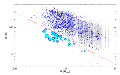
Figure 1: Distance as a function of stellar radius for the sample of planet hosts. All $10$ realizations are plotted here (gray dots). The CHARA R-band resolution limit ($0.24$ mas) is indicated with a red dashed line. Stars that are resolvable lie below this line. Blue dots indicate stars with measured $\sin{i_{\star}}$—i.e., those that pass our observational cuts in $v\sin{i_{\star}}$ and $P_{\rm rot}$ and have detectable photometric rotational modulation, as described in Section 5.1. Large cyan circles represent those stars that also pass the resolution, magnitude ($R<10$), and declination ($\delta>-30^{\circ}$) limits of the CHARA array—i.e., the subset with measured $\sin{i_{\star}}$ from directly measured diameters (Case (i)). The sizes of the circles are scaled logarithmically by their projected rotational velocities, which range from $2$ to $\mathord{\sim}120$ km s^-1.

We also point out that while citecite.sullivan:2015S15 treated stellar multiplicity with care to ensure realistic TESS planet yields, we do not explicitly include the effects of multiplicity in our calculations in the following sections. The primary effect is likely to be a small bias in some systems when fitting the photometric energy distribution to estimate radii, but we adopt conservative errors to mitigate this.

3.2 Calculating the Observable Quantities

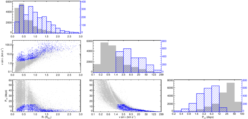
Figure 2: Comparison between the full sample of TESS planet hosts (gray) and the sample for which we expect $\sin{i_{\star}}$ measurements (blue). We show correlation plots and histograms for $R_{\star}$, $v\sin{i_{\star}}$, and $P_{\rm rot}$. The right (blue) axes in the histograms correspond to the measured $\sin{i_{\star}}$ sample, plotted as blue hatched histograms. All $10$ realizations of the planet simulations are plotted, and we have assumed $f_{\rm al}=0.7$ to generate the plotted $v\sin{i_{\star}}$ sample. It is clear that the smallest stars (slowest rotators) are most stongly affected by our observational cuts of ${v\sin{i_{\star}}}>2$ and ${P_{\rm rot}}<14$.

The stellar properties provided by citecite.sullivan:2015S15 include the distance modulus, $R_{\star}$, $T_{\rm eff}$, and absolute $V$ magnitude, which we can use to derive the observable quantities from Equation 2. We first trivially calculate $d$ from the distance modulus and $\Theta$ from $R_{\star}$ and $d$.

Next, we use the gyrochronological relation from Mamajek & Hillenbrand (2008) to calculate rotation periods:

$${P_{\rm rot}}=0.407\ [(B-V)-0.495]^{0.325}\ t^{0.566}$$ (4)

For this, we need the $B$ magnitudes, which we derive using the $T_{\rm eff}$–color table presented by E. Mamajek and Pecaut & Mamajek (2013). There is significant uncertainty in the four constants in Equation 4 (because real stars display a scatter about this relation), so we draw a new set of the four constants for each star, using the errors on these constants reported by the authors. This produces a stellar sample with a realistic scatter of rotation periods about the gyrochronological relation. We further note that the sample includes a handful of early type stars and a large number of M dwarfs, but the above relation is only calibrated for $0.5\mathrel{\hbox to0.0pt{\lower 4.0pt\hbox{\hskip 1.0pt$\sim$}\hss}\raise 1.0pt\hbox{$<$}}(B-V)\mathrel{\hbox to0.0pt{\lower 4.0pt\hbox{\hskip 1.0pt$\sim$}\hss}\raise 1.0pt\hbox{$<$}}0.9$ (F7-K2). Mamajek & Hillenbrand (2008) note that F3V–F6V spectral types appear to be where gyrochronology fails due to the thinning of convective envelopes and the loss of magnetic dynamos, thus preventing the magnetic braking from which spin-down laws emerge. These earlier types should therefore spin faster than their slightly less massive counterparts. As an approximation, we assign rotation periods for earlier types by assuming $(B-V)=0.5$, which may slightly overestimate the rotation periods for the hottest stars. For late-type dwarfs with $(B-V)>0.9$, we simply apply Equation 4 and acknowledge that these less massive, and in some cases fully convective, stars probably obey a somewhat different spin-down law. We argue that this is unlikely to significantly bias our results. Qualitatively, cooler stars will spin more slowly, so the declining rotation period relation should be correct to first order. Moreover, some very late-type stars are expected to have significant rotation—the predictable, monotonic spin-down seen in solar-type stars gives way to a bimodality for later types that includes both fast and slow rotators (e.g., Irwin et al., 2011; McQuillan et al., 2014). While this bimodality is most pronounced for the coolest stars, it begins to emerge even for stars as hot as $\mathord{\sim}4500$ K. At even lower masses, many brown dwarfs rotate with periods on the order of hours (e.g., Metchev et al., 2015, and references therein). In all cases, by erring toward overestimated rotation periods, we will also overestimate uncertainties for $P_{\rm rot}$ and $v\sin{i_{\star}}$, thereby obtaining more conservative results. That said, one must also worry that comparisons between observed data and simulated data could introduce systematically biased results if the properties of the simulated data do not reflect the properties of real stars. Since Equation 4 is expected to break down for late-type stars, we explore simulations of a more conservative sample selection — one for which gyrochronology is better suited — in Section 5.4.

A further complication in simulating $P_{\rm rot}$ is that measured rotation periods (including those used to derive gyrochronology relations) track the rotational velocity at the active spot latitudes rather than at the equator—the rotation periods we assigned are therefore the periods at the active latitudes. We can assign equatorial rotation periods by assuming a differential rotation law and spot latitude distribution. Following the approach of Hirano et al. (2014) and Morton & Winn (2014), we adopt the functional form for differential rotation from Collier Cameron (2007):

$${P_{\rm rot}}(\ell)=\frac{P_{\rm rot,eq}}{1-\alpha\sin^{2}\ell},$$ (5)

and we draw spot latitudes from a distribution $\ell=20\pm 20^{\circ}$, and assume the strength of differential rotation is similar to the Sun ($\alpha=0.23$).

Hirano et al. (2014) showed that differential rotation will similarly result in a measured $v\sin{i_{\star}}$ that is too large by a factor $\mathord{\sim}(1-\alpha/2)^{-1}$. While applying this correction to observations of real systems has the potential to introduce a small error if the true strength of differential rotation is significantly different from the assumed solar value of $\alpha=0.23$, in our simulations the true and observed values would both receive the same correction, so we ignore this small factor.

With the equatorial $P_{\rm rot}$ and $R_{\star}$ in hand, we can generate $v\sin{i_{\star}}$ by drawing $i_{\star}$ from an appropriate distribution. We note that an isotropic distribution is most likely not the correct choice for this distribution—our hypothetical planets all transit, so if $\psi$ is preferentially low (well-aligned), then $i_{\star}$ must be preferentially high (edge-on rotation). We explore the effect of different obliquity distributions in Section 5.

4 Assigning Uncertainties and Simulating Observations

4.1 Distance Uncertainty

The most uniform and complete set of distances currently available for nearby Sun-like stars (${<}100$ pc) comes from the Hipparcos mission (ESA, 1997). van Leeuwen (2007) quoted a mean parallax precision for single stars of $0.33$ mas for $H_{P}<7$ mag, and $0.56$ mas for $H_{P}<9$ mag, which corresponds to distance precisions of $\mathord{\sim}1\%$ for Sun-like stars at $30$ pc, and $\mathord{\sim}4\%$ for those at $75$ pc. For many of the fainter TESS targets, this uncertainty easily becomes the dominant term in the error budget of Equation 3. Fortunately, the Gaia mission (Perryman et al., 2001) promises to improve upon this considerably, by providing parallax measurements to roughly 1 billion stars; first estimates of these distances are expected to be available prior to the launch of TESS. de Bruijne (2012) quoted an anticipated precision of better than $10\ \mu$as for $G<12$ mag stars— corresponding to a distance precision better than $0.1\%$ at $100$ pc and better than $1\%$ at $1$ kpc—although faint stars and some very close visual binaries may carry additional measurement errors. Evaluation of in-orbit commissioning data suggests that despite some minor operational hiccups (e.g., significant stray light levels, larger than expected instability of the basic angle between the lines of sight of the two telescopes) the astrometric performance will remain within the $20\%$ science margin set before launch; the updated performance predictions given by de Bruijne et al. (2014) suggest that the majority of the TESS stars will carry a parallax error smaller than $\mathord{\sim}15\ \mu$as. We approximate distance errors by propagating a constant $15\ \mu$as uncertainty in parallax, $\sigma_{d}=15\times 10^{-6}d^{2}$ pc.

4.2 Stellar Angular Diameters: Available Populations and Uncertainties

Stellar angular diameters can either be measured directly from interferometric measurements or estimated from bolometric fluxes and effective temperatures: $\Theta^{2}=4F_{\rm bol}/(\sigma T_{\rm eff}^{4}$). Since the directly measured values translate to stellar inclinations with the smallest uncertainties, we consider this population first. For a star to be spatially resolved, it must be both bright enough for precise measurements and larger than the resolution limit. Currently the world’s longest baseline interferometer operating at optical and infrared wavelengths, where photospheres are the brightest, is Georgia State University’s CHARA Array, located on Mt. Wilson in California (ten Brummelaar et al., 2005). With a long baseline of $331$ m, the Array yields an angular resolution ($\lambda/2B$) of $0.51$ mas in the H band and $0.24$ mas in the R band; an adaptive optics system is currently being installed that is predicted to achieve limiting magnitudes of $9.0$ at H and $10.0$ at R (ten Brummelaar et al., 2012, 2014); current limiting magnitudes for precision measurements are $7.0$ and $7.0$, respectively.

To determine the number of stars that the CHARA Array is likely to spatially resolve, we adopt the R band adaptive optics limits of $\theta_{\rm res}=0.24$ mas and $R_{\rm lim}=10.0$ mag, and assume a declination limit of $\delta>-30^{\circ}$. These limits are applied to the $10$ realizations of the TESS simulated planetary population, and yield a mean of $14.8$ TESS transiting planet hosts resolvable by CHARA. This subset of stars is illustrated in Figure 1. We note that for all but the very latest types, the primary limitation is their small angular sizes, rather than their faint $R$ magnitudes; relative to the CHARA limits, the typical TESS planet host is small but not necessarily faint. The brightness of these stars will enable high signal-to-noise ratio observations that are important for achieving precise size measurements, and their small sizes are not an insurmountable obstacle; Huber et al. (2012), for example, obtained angular diameters to within $2\%$ for several bright stars close to (and even beyond) the nominal resolution limit using a modest number of observations. It thus seems plausible that the majority of these stars that are large enough and bright enough for CHARA to resolve and could have their sizes measured with similar precisions. We therefore adopt a $2\%$ uncertainty in directly measured angular diameters.

Since the subsample that can be spatially resolved with CHARA represents only a small fraction of the expected TESS planet hosts, we also consider the precision with which radii can be estimated. Boyajian et al. (2014) demonstrate that angular diameters can be predicted with a precision of $5\%$ from single color relations and an absolute magnitude, based on the dispersions about the best fit relation for nearby stars with interferometrically measured radii and Hipparcos distances. However, applying these relations blindly to TESS targets will likely yield biased results since the sample extends to distances of $\mathord{\sim}500$ pc (see Figure 1) and many stars likely experience modest extinction. There are two promising methods to account and correct for this. First, the precise distances that Gaia will provide, coupled with spectroscopically determined temperatures, will yield all sky extinction maps (Schultheis et al., 2015) and enable first order corrections. And for planet hosts with a spectroscopically determined temperature, their observed photometric energy distribution can be compared to that expected for their temperature to derive their line-of-sight extinction. Thus, with very accurate Gaia distances and extinction corrections, photometric energy distributions (as opposed to single color relations) can be used to get accurate bolometric fluxes. When combined with spectroscopically determined temperatures, these will yield accurate angular diameters via the Stefan–Boltzmann Law—$\Theta\propto\left(F_{\rm bol}\right)^{0.5}\left({T_{\rm eff}}\right)^{-2}$. We adopt a conservative $5\%$ uncertainty in estimated angular diameters, since that precision has already been demonstrated using single colors, but we expect that it should be possible to do better using the full photometric energy distribution.

4.3 Rotation Period Uncertainty

The photometric precision and high cadence ($\mathord{\sim}2$ minute) observations of TESS will enable the detection of a large number of stellar rotation periods. For example, McQuillan et al. (2014) report $34,\!000$ rotation periods among the Kepler sample, corresponding to a recovery rate of $\mathord{\sim}25\%$ for cool (${<}6500$ K) dwarfs without eclipsing binary companions.

The TESS and Kepler dwarf samples will differ in several ways, and while we discuss these differences below, we ultimately argue that adopting detection rates from the Kepler sample is justified in our simulations. Perhaps the most important difference between data sets will be the typical time span of observations for TESS stars. In general, they will not have the luxury of the long-term monitoring that Kepler provided—most TESS stars will be monitored for only $27.4$ days (one spacecraft pointing), though near the ecliptic poles, field overlap will allow $\mathord{\sim}1$ year of continuous monitoring. We therefore expect that precise rotation periods will only be determined for ${P_{\rm rot}}<14$ days, and remove slower rotators from our simulations. This observational constraint is likely to limit TESS detection of rotation periods mainly to stars younger or earlier-type than the Sun (i.e., rotating faster than $P_{\rm rot,\odot}\mathord{\sim}26$ days), and may hinder detections for slowly rotating late-type stars. However, in the context of Kepler rotation periods, the former limitation may not be important, as McQuillan et al. (2014) suggest that very few rotation periods of stars older than the Sun were detected. Similarly, in the context of Case (i) (interferometrically determined $\Theta$), relatively few late type stars will be resolvable because of their small sizes and large magnitudes; reduced sensitivity to rotation periods of late-type stars will have relatively little effect on the overall results. For Case (ii) (photometrically determined $\Theta$), TESS might not observe multiple full rotations for old or cool stars, which could hinder the application of IPR. However, the typical amplitudes of variation are large enough ($\mathord{\sim}1$ to $22$ mmag in the $5^{\rm th}$ to $95^{\rm th}$ percentile) that ground-based follow-up should in most cases be capable of determining the rotation periods. This would not be ideal, but is not an insurmountable obstacle.

Because TESS will observe the brightest stars in the sky, it is worth comparing TESS and Kepler photon noise. TESS targets will typically be $30$–$100$ times brighter than Kepler targets. However, the TESS aperture has an area $100$ times smaller than Kepler and photon noise will therefore generally be comparable to or greater than for Kepler. Kepler’s longer duration is also an asset to beat down noise, and the results will ultimately depend on the photometric precision TESS is able to achieve. The brightness of TESS targets will at least better enable ground-based follow-up, e.g., to determine or improve rotation periods of stars for which TESS does not observe many rotation periods.

We assume that the fractional uncertainties in the measured $P_{\rm rot}$ reported by McQuillan et al. (2014) are also roughly indicative of the precisions one can expect from TESS, at least for periods short enough to be determined reliably. This assumption may ultimately prove to be optimistic, so we also run simulations that adopt a more conservative $P_{\rm rot}$ error estimate in Section 5.4. Here, however, we assume that the combination of sophisticated analysis and photometric follow-up can provide rotation periods with precisions similar to those determined using Kepler data. Among $34,\!000$ main sequence Kepler stars for which McQuillan et al. (2014) detect rotation periods, the highest probability density (and $1\sigma$ error) of the fractional period uncertainty is $0.29\%^{+1.51\%}_{-0.29\%}$; the period uncertainty is on average dependent upon the rotation period itself. To account for this, we assign uncertainties as a function of rotation period using the McQuillan et al. (2014) catalog. For each bin in $P_{\rm rot}$, we calculate the probability density function (PDF) of the fractional uncertainty using a kernel density estimator. For each star in that bin, we then draw a fractional uncertainty according to the PDF, which is trivially converted to an absolute uncertainty, $\sigma_{P_{\rm rot}}$. One complication is that the observed rotation period is actually the period at the active spot latitude rather than equatorial rotation. To account for this we first simulate the observed rotation period, $\hat{P}_{\rm rot}(\ell)=P_{\rm rot}(\ell)+x\sigma_{P_{\rm rot}}$, and then assume $\ell=20^{\circ}$ in order to estimate the correction needed to determine the equatorial rotation period: $\hat{P}_{\rm rot}=\hat{P}_{\rm rot}(\ell)(1-\alpha\sin^{2}(20\ {\rm deg}))=0.973\hat{P}_{\rm rot}(\ell)$. The cumulative effect of having to estimate the active spot latitude correction is typically an additional error in the equatorial rotation period of $\mathord{\sim}2.5\%$ (stemming from the uncertainty in $\ell$) that is not included explicitly in the measurement errors for the observed rotation period.

4.4 Projected Rotational Velocity Uncertainty

The projected (equatorial) rotational velocities, $v\sin{i_{\star}}$, can be obtained from high resolution spectroscopy. Unlike $T_{\rm eff}$, $\log{g}$, and $\rm{[Fe/H]}$, $v\sin{i_{\star}}$ is mostly free from degeneracy with the other parameters. For stars rotating sufficiently fast such that rotation is the dominant broadening mechanism ($v\sin{i_{\star}}$$\gtrsim$ 10), $v\sin{i_{\star}}$ can typically be determined to a few percent with high signal-to-noise ratio, high dispersion spectra (e.g., Siverd et al., 2012; Bieryla et al., 2015). However, for more slowly rotating stars, complicating effects such as the assumed macroturbulent velocities of convective cells ($v_{\rm mac}$) can directly affect the predicted spectral line profiles. For example, the difference in derived $v\sin{i_{\star}}$ if one assumes $v_{\rm mac}$ values of $2$ and $3$ km s^-1 is $\mathord{\sim}0.25$ km s^-1, or $2.5\%$ for a star with $10$ km s^-1 total line broadening. There is hope that observationally calibrated relationships between $T_{\rm eff}$, $\log{g}$, and $v_{\rm mac}$ (e.g., the asteroseismically calibrated relationship presented by Doyle et al., 2014) can be used to constrain $v_{\rm mac}$ and mitigate such a bias. In practice, however, even with perfect knowledge of $v_{\rm mac}$, current typical measurement uncertainties for stars with ${v\sin{i_{\star}}}<10$ km s^-1 are $0.2-0.3$ km s^-1, and thus approach a $10\%$ uncertainty for stars with $v\sin{i_{\star}}$ values of only a few km s^-1 (e.g. Gray, 2013; Tsantaki et al., 2014). We note that some more sophisticated analysis techniques may improve the precision several fold (Gray & Baliunas, 1997) if measuring $v\sin{i_{\star}}$, as opposed to simply accounting for it in a stellar model, were the goal. Finally, measurement of $v\sin{i_{\star}}$ values that are less than the instrumental resolution are possible, but become even more challenging. The HARPS-N spectrograph (Cosentino et al., 2012), for example, has a resolving power of $R\mathord{\sim}115,\!000$, corresponding to a resolution element of $2.6$ km s^-1; if $v\sin{i_{\star}}$ is much slower than this, then it is only a minor contributor to the total line broadening. Large fractional changes in $v\sin{i_{\star}}$ therefore have relatively little effect on the line profiles and cannot be measured precisely. In these cases it is best to assign an upper limit on the $v\sin{i_{\star}}$ value, although a proper choice for this limit, relative to the instrumental resolution, is also data quality dependent.

Given the above considerations, we adopt the following uncertainties for $v\sin{i_{\star}}$. For stars with ${v\sin{i_{\star}}}\geq 10\ {\rm km\thinspace s^{-1}}$, we assume an uncertainty of $2.5\%$. For stars with $10\ {\rm km\thinspace s^{-1}}\geq{v\sin{i_{\star}}}\geq 2\ {\rm km\thinspace s^{-1}}$, we assume a constant uncertainty of $0.25$ km s^-1, which corresponds to an uncertainty of $2.5\%$ at $10$ km s^-1 and $12.5\%$ at $2$ km s^-1. For stars with ${v\sin{i_{\star}}}<2$ km s^-1, we assume that only an upper limit can be inferred, and we remove these stars from our sample.

We acknowledge that much of the exoplanet literature quotes larger errors for slow rotators (often $\pm 0.5$ km s^-1), but we point out that this convention has arisen because the effort and/or telescope resources required to push toward more precise $v\sin{i_{\star}}$ would usually provide diminishing scientific returns; in most cases, improving the $v\sin{i_{\star}}$ precision would not affect the conclusions of the paper at all, so a adopting a conservative error makes sense. Achieving our assumed uncertainties may be a difficult pursuit, but it is one that is feasible with current techniques and in the context of this work, the scientific returns would be well worth the effort. Finally, we note that a concerted effort to make these measurements would not have to be carried out for all TESS hosts, but only the much smaller number to which IPR can be applied.

4.5 Simulating Measured Quantities

To determine which, and how many, systems will be amenable to projected obliquity measurements via IPR, we simulate observations of each star in our sample to arrive at simulated observed values of ${\sin{i_{\star}}}$. This simulated observed distribution has two uses. First, it can be populated with transiting planets according to realistic occurrence rates in order to calculate the likely yield of projected obliquities (and their distribution and uncertainties). Second, by running this simulation many times, we can build well-sampled, expected distributions of observed ${\sin{i_{\star}}}$ values under various assumptions (number and characteristics of survey targets, observational uncertainties and limits, etc.). These distributions can be used as comparison samples against which we can compare our observed distributions (e.g., in a Kolmogorov–Smirnov test). This will therefore allow us to test observed distributions against arbitrary underlying obliquity distributions.

We first point out that measurement precision as a function of stellar properties is somewhat nuanced, as the precision of several of the observables is expected to have a dependence on other stellar properties. We therefore must be careful when simulating observed quantities and their measurement uncertainties. Very generally, given the observable quantities $p=\{d,\Theta,{P_{\rm rot}},{v\sin{i_{\star}}}\}$ with true values $p_{i}$ as calculated in Section 3, we need to assign for each star in our sample the observed values, $\hat{p}_{i}$, and uncertainties, $\sigma_{p_{i}}$. Under the assumption of uncorrelated Gaussian errors, these quantities can be related simply by:

$$\hat{p}_{i}=p_{i}+x\sigma_{p_{i}},$$ (6)

where $x$ is drawn from a normal distribution, $x\mathord{\sim}\mathcal{N}(0,1)$.

Using the above relation we can simulate measured quantities for $d$, $\Theta$, and ${P_{\rm rot}}$. Simulating measurements of $v\sin{i_{\star}}$, however, requires assigning a distribution of $i_{\star}$ values, which are unlikely to be random for stars that host transiting planets. For example, if most planets are coplanar with the stellar equator, then for a sample of transiting planets, the underlying inclination distribution should be confined to near-$90^{\circ}$ orientations. However, if all systems experience significant evolution of their angular momenta, an isotropic distribution might be more appropriate. The true distribution may contain a mix of systems: well-aligned systems that have formed in an equatorial disk and experienced calm migration (or no migration at all), plus a more isotropic distribution caused by interaction of the planets or proto-planetary disk with a binary or additional planetary companions. For Case (i) (interferometric $\Theta$), we do not expect a large number of systems (or a powerful population analysis), and we thus confine our investigation to two simple inclination distributions: isotropic, in which the probability of observing a particular inclination is given by $P(i_{\star})\mathord{\sim}\cos{i_{\star}}$; and well-aligned, which we characterize as an isotropic distribution truncated to within $10^{\circ}$ of alignment. For Case (ii) (photometric $\Theta$), we expect many more systems, and therefore anticipate that we will be able to distinguish much more finely between underlying distributions. We therefore simulate many "mixed" distributions, comprised of varying fractions of the above isotropic and aligned distributions. We refer to these mixed distributions by the fraction of aligned systems—for a mixed distribution with $f_{\rm al}=0.7$, $70\%$ of systems are drawn from an aligned distribution and $30\%$ of systems are drawn from an isotropic distribution. Regardless of the distribution from which $i_{\star}$ is drawn, our observed projected rotational velocities are simply given by $\hat{v}{\sin{i_{\star}}}={v\sin{i_{\star}}}+x\sigma_{v\sin{i_{\star}}}$ (with $\sigma_{v\sin{i_{\star}}}$ chosen as outlined in Section 4.4).

For a given distribution of $i_{\star}$ values, all four measured quantities can be simulated and the uncertainty in $\sin{i_{\star}}$ can be determined from formal error propagation.

4.6 Resulting Uncertainty on the Stellar Inclination

As described in more detail above, a typical spatially resolvable star might have errors of $\sigma_{P_{\rm rot}}\mathord{\sim}1\%$, $\sigma_{\theta}\mathord{\sim}2\%$, and $\sigma_{d}\mathord{\sim}0.1\%$, with an additional $\mathord{\sim}2.5\%$ uncertainty in $\sigma_{P_{\rm rot}}$ introduced by correcting for differential rotation. The fractional error on $v\sin{i_{\star}}$ depends on $v\sin{i_{\star}}$ itself; for the example of a star rotating at $5\pm 0.25$ km s^-1 ($\sigma_{v\sin{i_{\star}}}\mathord{\sim}5\%$), this combination of uncertainties leads to $\sigma_{\sin{i_{\star}}}\mathord{\sim}6\%$. The corresponding constraint on $i_{\star}$ would depend on the inclination: for nearly edge-on rotation ($\sin{i_{\star}}\mathord{\sim}1$), one would derive an uncertainty in $i_{\star}$ of $\mathord{\sim}20^{\circ}$, but for lower stellar inclinations, the uncertainty may be only a few degrees. Thus, individual well-aligned systems will still be difficult to identify with confidence—especially around slow rotators for which the $v\sin{i_{\star}}$ fractional uncertainty is large—but misaligned systems should result in highly significant detections and precise measurements. Despite this difficulty for some individual systems, the population of ${\sin{i_{\star}}}$ measurements should be able to constrain the underlying obliquity distribution, and the smaller uncertainties resulting from IPR using precise distances and angular diameters should reduce the number of measurements required to do so.

5 Results

5.1 Expected Number of Obliquity Measurements

The above discussion quantifies how well the stellar inclination can be determined in any one case, and the simulated stellar population allows us to estimate the number of transiting systems for which these projected obliquity measurements can be realized. This number can be estimated by multiplying the initial number of targets successively by the fraction that hosts planets, the fraction for which a transit is detected, and the fraction that has detectable rotational modulation and rotational line broadening:

$$N_{\rm ob}=N_{\star}\times f_{\rm pl}\times p_{\rm tr}\times f_{\rm rot}.$$ (7)

By using their simulated TESS planet catalog, we have implicitly adopted the first three terms from citecite.sullivan:2015S15; briefly, they assume $N_{\star}=200,\!000$ and assign planet occurrence rates ($f_{\rm pl}\times p_{\rm tr}$) as a function of stellar properties and orbital period using the Kepler planet occurrence statistics reported by Fressin et al. (2013) and Dressing & Charbonneau (2013, 2015). Given the mean number of planets from $10$ realizations of the citecite.sullivan:2015S15 simulations, Equation 7 becomes $N_{\rm ob}=1863\times f_{\rm rot}$.

Not all stars are active enough to reveal their rotation periods, and activity level varies as a function of spectral type, so we cannot adopt a single value for $f_{\rm rot}$ in our simulations. Additionally, our fiducial simulation makes the assumption that $v\sin{i_{\star}}$ cannot be measured below $2$ km s^-1 and that rotation periods longer than $14$ days will not be identified by TESS, so systems that do not satisfy these criteria will be removed, even if the photometric amplitude of rotational modulation is expected to be detectable. To assess detectability of rotational modulation, we first assume that TESS will recover rotation periods at the same rate as Kepler. McQuillan et al. (2014) detected rotation in $83\%$ of cool stars (${<}4000$ K), but in only $\mathord{\sim}20\%$ of stars hotter than the Sun. To enforce this condition, we divide our sample into bins of $100$ K in $T_{\rm eff}$ and then flag stars as detectable with probability according to the PDF of the McQuillan et al. (2014) rotation periods in that $T_{\rm eff}$ bin, normalized to the detection rate for that $T_{\rm eff}$. In this way, our final distributions of rotation periods and detection rates as a function of $T_{\rm eff}$ broadly match the Kepler sample before we apply our observational cuts of ${P_{\rm rot}}<14$ days and ${v\sin{i_{\star}}}>2$ km s^-1. Finally, we note that the fraction of transiting planet host stars with ${v\sin{i_{\star}}}>2$ km s^-1 depends upon the underlying obliquity distribution: well-aligned systems will have larger $v\sin{i_{\star}}$ on average. This effect is seen in the results of our simulations. After assessing $P_{\rm rot}$ detectability and applying the observational cuts, we estimate $N_{\rm ob}\mathord{\sim}189$ for an isotropic distribution of obliquities and $N_{\rm ob}\mathord{\sim}214$ for a well-aligned distribution.

We compare the properties of the full planet host sample to those of the “measured $\sin{i_{\star}}$” sample in Figure 2. One can clearly see the primary result of the observational limits we have imposed: the excluded slow rotators tend to be the smallest stars, so the “measured $\sin{i_{\star}}$” sample is biased toward larger (more massive) stars than the full planet host sample. Furthermore, the M dwarfs for which $\sin{i_{\star}}$ will be measured belong to the rapidly rotating subset of M dwarfs, which may indicate comparative youth or perhaps more fundamental differences. The properties of planetary systems orbiting these stars may therefore not be representative of all M dwarf planets. This will be important to keep in mind when interpreting results. This also highlights an opportunity – the extension of observational limits to smaller $v\sin{i_{\star}}$ and larger $P_{\rm rot}$ through improved techniques and follow-up observations will provide a larger and more representative population for this analysis. We discuss this opportunity further in Section 6.

5.2 Constraints on the Underlying Obliquity Distribution from Interferometric Measurements

The discussion in Section 5.1 considers the large sample of Case (ii) (photometrically derived angular diameters), but the (small) number of CHARA-resolvable TESS planet hosts can also be determined directly from the distances and radii provided by the citecite.sullivan:2015S15 simulations. A mean of $14.8$ resolvable planet hosts are expected, but only $2.2$ (isotropic distribution) or $2.5$ (aligned distribution) are expected to have ${v\sin{i_{\star}}}>2$ km s^-1 and a detected ${P_{\rm rot}}<14$ days.

A handful of projected obliquity measurements is not sufficient for a population analysis, but this group of planetary systems is likely to be well-studied, since uncertainties in stellar properties are most often the strongest limitation on our understanding of the properties of transiting planets, and the precision afforded by directly measured radii allows greater insights into processes governing the structure and evolution of both stars and planets (e.g., Boyajian et al., 2015). It is therefore plausible that through careful follow-up observations, another handful of these $\mathord{\sim}15$ systems will have rotation periods and rotational velocities measured, even beyond the $14$ day and $2$ km s^-1 limits assumed above. In any case, for a strong constraint on the underlying obliquity distribution, we must turn to the larger sample of photometrically derived angular diameters.

5.3 Constraints on the Underlying Obliquity Distribution from Photometric Measurements

Determining $\Theta$ from the photometric energy distribution or color relations will be harder to apply to individual systems because of its less precise measurements, but it holds greater promise as a means to probe the population as a whole because we expect hundreds of systems to be amenable to this technique. We describe here one methodology that can be used to characterize the true obliquity distribution and demonstrate it using our simulated observations of TESS planet hosts.

Given an underlying obliquity distribution, one may simulate a stellar and planetary population and a set of observations of those systems in order to construct the distribution of $\sin{i_{\star}}$ values that one expects to recover through observation. We refer to this as the “expected distribution”. It is a distribution corresponding to the true underlying distribution once it has been subjected to our observational constraints (i.e., ${v\sin{i_{\star}}}>2$ km s^-1, ${P_{\rm rot}}<14$ days) and measurement errors. This expected distribution can then be used as a comparison against the $\sin{i_{\star}}$ distribution that arises from observations of TESS systems—the “observed distribution”. (Since TESS has not yet launched, we also simulate the observed distribution here, of course.) To constrain the true underlying distribution, we run a series of Kolmogorov–Smirnov (KS) tests to characterize the similarity between the observed distribution (for a given value of $f_{\rm al}$) and many expected distributions (for many different values of $f_{\rm al}$). For pairs with $p<0.05$ ($<5\%$ chance that the same parent distribution would produce both the observed and expected distributions), we consider the distributions inconsistent. For a given observed distribution, we report the best fit as the expected distribution with the largest $p$-value and assign errors to encompass the expected distributions that produced $p>0.05$. Figure 3 illustrates this comparison for our fiducial simulations and a range of underlying obliquity distributions. The results are summarized in Table 1. It can be seen clearly that the best fit distribution does indeed accurately recover the distribution from which our systems were drawn.

One advantage of the technique outlined herein is that by simulating the stellar sample, the observations, and ultimately the expected distribution, the observed distribution can be tested against any model distribution, and the expected distribution captures the observational biases that would not be accounted for in a direct fit to an assumed functional form for the true distribution. In practice, it makes sense to test physically motivated distributions—such as our examples that have been parametrized to include $f_{\rm al}$ aligned systems and $1-f_{\rm al}$ isotropic systems, or the Fisher distribution favored by Morton & Winn (2014)—but the model distributions need not be parametric, and the use of the KS test to reject model distributions allows a fully non-parametric analysis. One could, for example, directly use the results of arbitrarily complex dynamical evolution models as the comparison distributions.

A potential drawback to this technique is that the reported errors from the grid of KS tests are difficult to interpret in a standard way. To investigate how realistic the errors are, we also fit the observed cumulative distribution function (CDF) directly to a model CDF. For nodes in the observed CDF located at $(\hat{x},\hat{y})$, the corresponding nodes in the model CDF are located at $(\hat{x},y)$. The model CDF is taken to be a linear combination of aligned and isotropic CDFs:

$$\begin{split}{\bm{y}}(\hat{\bm{x}};f_{\rm al})&=\frac{1}{\beta}\Big{(}\alpha_{1}f_{\rm al}\ {\bm{y}}(\hat{\bm{x}};1)+\alpha_{0}(1-f_{\rm al})\ {\bm{y}}(\hat{\bm{x}};0)\Big{)};\\ \beta&=\alpha_{1}f_{\rm al}+\alpha_{0}(1-f_{\rm al}),\end{split}$$ (8)

where the $\alpha$ terms are weight parameters to account for more obliquities being measured in aligned distributions, and $\beta$ is simply the normalization. We fit to minimize $\chi^{2}$, with errors for the observed CDF at a given $\sin{i_{\star}}$ value assigned to be proportional to the square root of the $\sin{i_{\star}}$ PDF (equivalent to counting statistics), and scaled so that $\chi^{2}_{\rm red}=1$. The $1$-$\sigma$ errors from this direct fit, corresponding to the central $68.3\%$ highest probability density region, are typically about $\pm 0.09$. These errors roughly correspond to the errors one would get from the KS grid by assuming the $1$-$\sigma$ region is well-described by $p>0.317$. We therefore conclude that our reported errors are, if anything, conservative. We choose to retain the larger errors, as potential systematics in our method (discussed in Section 6) may reduce accuracy for real observations.

Based on these simulations, we conclude that the expected yield of projected obliquity measurements from TESS will enable identification of the likely true obliquity distribution for hosts of planets of all sizes. In our example—motivated by migration processes that might be expected to produce a bimodal distribution of obliquities (i.e., aligned or isotropic, depending on the migration mechanism or lack thereof)—TESS obliquities should determine the fraction of systems drawn from a well-aligned distribution to within $\mathord{\sim}0.15$. The results of such an analysis holds insight into the relative importance of various proposed formation and migration mechanisms.

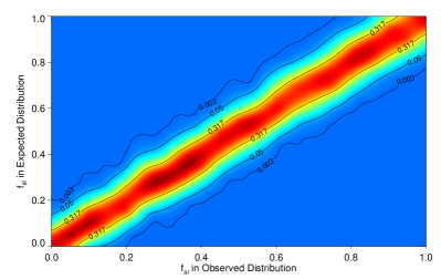
Figure 3: KS test $p$-values (colored contours) for observed and expected $\sin{i_{\star}}$ distributions comprised of $f_{\rm al}$ well-aligned systems (and $1-f_{\rm al}$ randomly oriented systems). Low $p$-values (blue regions) correspond to pairs of expected and observed distributions that are unlikely to arise from the same parent distribution. The most likely true fraction of aligned systems is that for which the expected distribution produces the largest $p$-value (red regions), and the distance over which the $p$-values decline characterizes the precision with which the true aligned fraction can be measured. For each observed distribution, we adopt the region with $p>0.05$ (red to cyan) as the uncertainty on $f_{\rm al}$ for the true underlying distribution. The results are summarized numerically in Table 1.

Table 1:
Constraints on the Underlying Obliquity Distribution

$f_{\rm al}$ drawn	$f_{\rm al}$ derived
${\kern-28.45274pt}0\%$	$0^{+14}_{-0}\%{\kern-28.45274pt}$
${\kern-28.45274pt}10\%$	$10^{+15}_{-10}\%{\kern-28.45274pt}$
${\kern-28.45274pt}20\%$	$20^{+15}_{-14}\%{\kern-28.45274pt}$
${\kern-28.45274pt}30\%$	$30^{+15}_{-14}\%{\kern-28.45274pt}$
${\kern-28.45274pt}40\%$	$40^{+14}_{-16}\%{\kern-28.45274pt}$
${\kern-28.45274pt}50\%$	$50^{+15}_{-15}\%{\kern-28.45274pt}$
${\kern-28.45274pt}60\%$	$60^{+16}_{-14}\%{\kern-28.45274pt}$
${\kern-28.45274pt}70\%$	$70^{+16}_{-14}\%{\kern-28.45274pt}$
${\kern-28.45274pt}80\%$	$80^{+16}_{-15}\%{\kern-28.45274pt}$
${\kern-28.45274pt}90\%$	$90^{+10}_{-15}\%{\kern-28.45274pt}$
${\kern-28.45274pt}100\%$	$100^{+0}_{-16}\%{\kern-28.45274pt}$

Note. — For each distribution from which we draw an observed sample (given in the first column and specified by the fraction of aligned systems in the distribution), we show the derived underlying distribution (see Section 5.3 and Fig. 3 for details). The population of $\sin{i_{\star}}$ measurements expected from the pre-selected TESS targets accurately recovers the correct distribution.

5.4 A More Conservative Simulation

As described in Section 4, the simulations presented to this point rely upon a number of assumptions about our understanding of stellar populations, achievable measurement precisions, and the power of analysis techniques that may in some cases be described as optimistic. In this section, we identify two of the more optimistic assumptions that we have made and we describe and summarize a second set of simulations in which we temper those assumptions and present a more conservative outlook for the application of IPR to TESS planetary systems.

At the heart of the technique we have outlined is the assumption that we can generate realistic $\sin{i_{\star}}$ distributions for the TESS stellar population. If our simulated stellar properties do not reflect reality, we may be introducing a systematic bias to our final results. In this context, we may worry about applying the gyrochronology relation of Equation 4 to stars outside of its intended color range. In particular, we apply this relation to generate rotation periods of late-type stars, but as discussed in Section 3, stars cooler than about $5000$ K are not expected to obey this relation. While this assumption leads to conservative rotation period errors, it almost certainly also leads to a slightly unrealistic distribution of rotation periods, which may bias final results. In our conservative simulations, we therefore remove from the sample all host stars cooler than $5000$ K. While these stars are numerous within the TESS parent sample, our previously imposed cuts requiring ${v\sin{i_{\star}}}>2\ {\rm km\thinspace s^{-1}}$ and ${P_{\rm rot}}<14$ days had already removed the vast majority of late-type stars. Nevertheless, because the fraction of systems displaying detectable photometric rotational modulation is much larger for late-type stars, they did represent about $35\%$ of the systems for which we expected to measure $\sin{i_{\star}}$. These conservative simulations therefore predict only about $130$ (instead of $\mathord{\sim}200$) measured $\sin{i_{\star}}$ values.

In addition to limiting the number of stars we include, we also consider the measurement uncertainties we assign to our observations. For example, we have assumed that TESS rotation periods will be determined as precisely as Kepler rotation periods. While the typical photon noise should be similar, TESS targets will only be observed for $27.4$ days per pointing, so they will not have the benefit of years-long observations. To estimate the TESS rotation period precisions, we simulate TESS photometric data sets with white noise of $200$ ppm, a cadence of $2$ minutes, and a duration of $27.4$ days. We vary spot latitudes and amplitudes, and stellar inclinations and rotation periods out to $14$ days, and we attempt to measure rotation periods by fitting the peaks of the autocorrelation function (see McQuillan et al., 2014). We confirm that for the typical photometric amplitudes observed by Kepler, we can recover the correct period, and we calculate a measurement precision that depends almost entirely on the rotation period itself (as was found by McQuillan et al., 2014). Our simple light curve simulations do not consider multiple spot groupings, potential instrumental systematics, or contamination from other stars in the aperture, so errors may be somewhat larger than our analysis predicts. There are also factors that may improve precisions (e.g., a more sophisticated analysis, the contribution of ground-based follow-up, or the fact that a large number of planet hosts will actually lie in fields observed by TESS for as long as a year), but we nevertheless inflate our calculated precisions by a factor of four in an attempt to qualitatively account for additional sources of uncertainty in $P_{\rm rot}$. The result is that we adopt $\sigma_{P_{\rm rot}}$ approaching $5\%$ for rotation periods near $14$ days (compared to ${P_{\rm rot}}\lesssim 1\%$ for similar stars in the Kepler sample).

Using these revised sample selection criteria and $P_{\rm rot}$ errors, we repeat the experiment described in previous sections to determine the precision with which we can differentiate the underlying obliquity distribution using a set of observed $\sin{i_{\star}}$ measurements. Despite the reduced sample size and precisions with which we can determine $P_{\rm rot}$, we again find promising results: we estimate that even in these more conservative simulations, $f_{\rm al}$ can be determined to within better than $0.2$. How such a promising result is obtained is not immediately obvious, but can be explained fairly easily. While our sample was reduced in size and individual measurement precision, the stars that were ultimately lost from the sample provided the least information about the underlying distribution. These cool stars are the ones with the slowest rotational velocities, and consequently the largest fractional uncertainties on their $v\sin{i_{\star}}$ measurements and the most poorly determined $\sin{i_{\star}}$ values. Their inclusion in the observed $\sin{i_{\star}}$ distribution therefore improves the counting statistics but smears the shape, both of which are used to distinguish between simulated distributions. As a result, removing a large number of them from the sample, as we have done in these conservative simulations, only slightly reduces the information in the $\sin{i_{\star}}$ distribution.

6 Applications and Improvements

While we have demonstrated the value of the IPR technique using precise Gaia distances and angular diameters (rather than estimated linear radii) for TESS transiting planets, it can easily be applied to other surveys and other types of systems. For example, Kepler systems can be examined almost immediately upon release of Gaia distances, as the planets and rotation periods have already been identified (with occurrence and detection rates well-understood), $v\sin{i_{\star}}$ measurements have already been made, and broadband photometry exists for most stars in the field. Similarly, as the two-wheeled Kepler mission (K2) continues to survey the ecliptic plane, the requisite data should become available. Furthermore, the all-sky TESS FFIs should enable detection of more planets than will observations of the pre-selected target stars (see citecite.sullivan:2015S15). Observations will be more difficult for these fainter stars, and measurement errors will be larger, but these samples should eventually contribute significantly to constraints on host star obliquities.

One caveat is that to apply IPR in the manner we have presented—to constrain the underlying obliquity distribution—one needs to understand the target sample and detection probabilities well enough to simulate an accurate stellar and planetary population. In addition, a large observing program would need to be undertaken to obtain high signal-to-noise, high resolution spectra of the planet hosts with known rotation periods in order to measure $v\sin{i_{\star}}$ (and $T_{\rm eff}$ for calculating $\Theta$ via $F_{\rm bol}$). Much of this data already exists for Kepler targets (and now K2 targets), and has been provided by the Kepler team and members of the broader exoplanet community as part of the Community Follow-up Observing Program (CFOP), but additional uncertainties may be introduced by the multiple instruments used and widely varying quality of the spectra. While another community effort will be most likely to provide the requisite data, an observing program dedicated to the task would ideally be carried out on a single suitable instrument. We note here that while the TESS target list and expected number of planet hosts are daunting, these observations would only need to be carried out for the $\mathord{\sim}200$ systems amenable to this analysis.

As for applying IPR to individual systems, the sky-plane projected obliquities have been measured for many hot Jupiters via the Rossiter–McLaughlin effect, and combination with the line-of-sight projection via IPR should, in some cases, provide the true obliquity, especially when using precise Gaia distances and angular diameters rather than radius estimates from stellar models.

It should also be noted that the orientation of angular momenta is an interesting diagnostic not only for short-period transiting planets. The same method can be used for eclipsing binaries, or even for non-transiting planets or debris disk systems. Directly imaged planet hosts, for example, tend to be bright, young, large, and nearby, all of which improve the measurements needed for IPR: young stars tend to rotate more rapidly (leading to precise $v\sin{i_{\star}}$) and with larger amplitudes (leading to easy $P_{\rm rot}$ detection), and their brightness, size, and proximity make them easily resolvable. While the orientation of the planet or disk is not limited to an edge-on orientation as is the case for transiting systems, if a planet shows an orbital arc, its orbital inclination can be constrained, and one could therefore probe angular momenta in planetary populations at wide separations. Similarly, debris disk orientation in relation to the stellar spin axis can constrain the primordial alignment in planetary systems.

Though the potential applications of IPR are exciting, the biggest hurdles will be improving measurement precision (thereby improving individual system obliquity determinations as well as the power of population analyses) and eliminating systematic uncertainties that might bias our results. In most cases, $v\sin{i_{\star}}$ is the limiting factor because slow rotation is difficult to measure precisely. Using ultra-high resolution spectrographs could reduce the error contributions from $v\sin{i_{\star}}$ (although this would increase observing costs), as could analysis techniques developed specifically for precise $v\sin{i_{\star}}$ determination, which has not typically been a goal in the exoplanet literature. Such improvements may also justify inclusion of more slowly rotating stars in our sample, perhaps down to $1.5$ or $1.0$ km s^-1, leading to a larger sample of obliquities around a wider range of spectral types, and therefore a more powerful, less biased population analysis. As we also demonstrated in the conservative simulations of Section 5.4, the precision of the measurements is as important as the sample size, and because $v\sin{i_{\star}}$ is the limiting factor for many systems—particularly low-mass hosts—improvements to $v\sin{i_{\star}}$ measurements would have a large effect on the power of IPR and would enable a study of obliquities across a wider range of stellar masses. Making use of extremely precise distances and color-angular diameter relations, stellar radius measurements can already be delivered to within $\mathord{\sim}5\%$, but using the full energy distribution to calculate the bolometric flux should in principle be better—careful development of this technique should also improve IPR. For TESS stars, rotation period measurements will be limited in most pointings to $<30$ days (and will not be precisely determined unless multiple periods are observed), but rotational variables can be identified and followed up from the ground since the stars will be so bright. This can again expand the sample for improved analysis and improve the $P_{\rm rot}$ precisions.

As measurement precisions increase, the method presented herein to constrain the true obliquity distribution of exoplanets will likely be limited by systematic uncertainties in the assumptions made while simulating $\sin{i_{\star}}$ distributions (e.g., that gyrochronology can predict rotation periods, or that macroturbulence can be accounted for correctly using $T_{\rm eff}$–$\log{g}$–$v_{\rm mac}$relations). That is, we have compared simulated observed and expected measurements under the same assumptions. If our assumptions contain a systematic bias, this is removed by comparing it against itself, but an analysis that compares against real observations will inherit that bias. In particular, differential rotation, macroturbulence, and stellar rotational evolution remain complicating (potentially systematic) factors. If typical spot latitudes and differential rotation strength can be well-characterized as a function of stellar properties, errors associated with rotation can be mitigated. Similarly, if characterization of macroturbulence as a function of stellar properties continues to improve, we can eliminate additional systematics in $v\sin{i_{\star}}$ measurements. The study of gyrochronology (and departures from standard spin-down laws) remains a very active field, further enabled by the same space missions with which we search for planets. Continued improvements in these areas of stellar astrophysics will benefit many areas of study, including that of planetary system architectures.

7 Summary

Measurements of the obliquities of the hosts of short-period giant planets have proven invaluable to the interpretation of their orbital evolution—the wide range of obliquities that has been observed is suggestive of an active dynamical past for the migrating planets and/or primordial planet-forming system. Initial results for small planets suggest that these systems are more likely than their larger counterparts to be flat, perhaps suggestive of a different dominant migration mechanism or in situ formation. However, comparatively little is known about the spin-orbit alignment for small planets—a large sample of obliquities for small planet hosts could lend strong evidence to the debate over in situ formation, the prevalence of primordially tilted disks, and the importance of wide companions in producing significant obliquity. We have presented a method to obtain such a sample by measuring the stellar inclinations of TESS planet hosts. To do so, we take advantage of an improvement in radius measurements made possible by precise distances that will be released by Gaia and angular diameters measured directly via interferometry or estimated from broadband photometry. Our simulations indicate that an analysis like the one presented here should be able to differentiate relatively finely between possible underlying obliquity distributions. In the example provided—in which the underlying distribution is modeled as a mixture of a fraction $f_{\rm al}$ aligned systems and ($1-f_{\rm al}$) randomly oriented systems—we expect an uncertainty in the derived aligned fraction of only $\sigma_{f_{\rm al}}\mathord{\sim}0.15$ ($\mathord{\sim}0.20$ under more conservative assumptions).

This technique will also be applicable to Kepler planets, results from K2 and ground-based surveys, eclipsing binaries, and directly imaged planets and disks, though it will be most useful as a population analysis for large samples. Finally, we point out that the power of this method can be improved by making precise measurements of $v\sin{i_{\star}}$, by furthering our understanding of stellar rotation and macroturbulence, and by carefully calibrating angular diameters derived from photometry.

References

- Albrecht et al. (2012a) Albrecht, S., Winn, J. N., Butler, R. P., et al. 2012a, ApJ, 744, 189
- Albrecht et al. (2012b) Albrecht, S., Winn, J. N., Johnson, J. A., et al. 2012b, ApJ, 757, 18
- Ballard & Johnson (2016) Ballard, S., & Johnson, J. A. 2016, ApJ, 816, 66
- Barnes et al. (2011) Barnes, J. W., Linscott, E., & Shporer, A. 2011, ApJS, 197, 10
- Bate et al. (2010) Bate, M. R., Lodato, G., & Pringle, J. E. 2010, MNRAS, 401, 1505
- Batygin & Adams (2013) Batygin, K., & Adams, F. C. 2013, ApJ, 778, 169
- Bieryla et al. (2015) Bieryla, A., Collins, K., Beatty, T. G., et al. 2015, AJ, 150, 12
- Boyajian et al. (2015) Boyajian, T., von Braun, K., Feiden, G. A., et al. 2015, MNRAS, 447, 846
- Boyajian et al. (2014) Boyajian, T. S., van Belle, G., & von Braun, K. 2014, AJ, 147, 47
- Broeg et al. (2013) Broeg, C., Fortier, A., Ehrenreich, D., et al. 2013, in European Physical Journal Web of Conferences, Vol. 47, European Physical Journal Web of Conferences, 03005
- Chaplin et al. (2013) Chaplin, W. J., Sanchis-Ojeda, R., Campante, T. L., et al. 2013, ApJ, 766, 101
- Chiang & Laughlin (2013) Chiang, E., & Laughlin, G. 2013, MNRAS, 431, 3444
- Collier Cameron (2007) Collier Cameron, A. 2007, Astronomische Nachrichten, 328, 1030
- Collier Cameron et al. (2010) Collier Cameron, A., Bruce, V. A., Miller, G. R. M., Triaud, A. H. M. J., & Queloz, D. 2010, MNRAS, 403, 151
- Cosentino et al. (2012) Cosentino, R., Lovis, C., Pepe, F., et al. 2012, in Proc. SPIE, Vol. 8446, Ground-based and Airborne Instrumentation for Astronomy IV, 84461V
- Dawson (2014) Dawson, R. I. 2014, ApJ, 790, L31
- de Bruijne (2012) de Bruijne, J. H. J. 2012, Ap&SS, 341, 31
- de Bruijne et al. (2014) de Bruijne, J. H. J., Rygl, K. L. J., & Antoja, T. 2014, in EAS Publications Series, Vol. 67, EAS Publications Series, 23
- Désert et al. (2011) Désert, J.-M., Charbonneau, D., Demory, B.-O., et al. 2011, ApJS, 197, 14
- Doyle et al. (2014) Doyle, A. P., Davies, G. R., Smalley, B., Chaplin, W. J., & Elsworth, Y. 2014, MNRAS, 444, 3592
- Dressing & Charbonneau (2013) Dressing, C. D., & Charbonneau, D. 2013, ApJ, 767, 95
- Dressing & Charbonneau (2015) —. 2015, ApJ, 807, 45
- Dumusque (2014) Dumusque, X. 2014, ApJ, 796, 133
- ESA (1997) ESA, ed. 1997, ESA Special Publication, Vol. 1200, The HIPPARCOS and TYCHO catalogues. Astrometric and photometric star catalogues derived from the ESA HIPPARCOS Space Astrometry Mission
- Fabrycky et al. (2014) Fabrycky, D. C., Lissauer, J. J., Ragozzine, D., et al. 2014, ApJ, 790, 146
- Fang & Margot (2012) Fang, J., & Margot, J.-L. 2012, ApJ, 761, 92
- Fielding et al. (2015) Fielding, D. B., McKee, C. F., Socrates, A., Cunningham, A. J., & Klein, R. I. 2015, MNRAS, 450, 3306
- Fressin et al. (2013) Fressin, F., Torres, G., Charbonneau, D., et al. 2013, ApJ, 766, 81
- Girardi et al. (2005) Girardi, L., Groenewegen, M. A. T., Hatziminaoglou, E., & da Costa, L. 2005, A&A, 436, 895
- Gray (2013) Gray, D. F. 2013, AJ, 146, 29
- Gray & Baliunas (1997) Gray, D. F., & Baliunas, S. L. 1997, ApJ, 475, 303
- Groot (2012) Groot, P. J. 2012, ApJ, 745, 55
- Hansen & Murray (2012) Hansen, B. M. S., & Murray, N. 2012, ApJ, 751, 158
- Hirano et al. (2012) Hirano, T., Sanchis-Ojeda, R., Takeda, Y., et al. 2012, ApJ, 756, 66
- Hirano et al. (2014) —. 2014, ApJ, 783, 9
- Huber et al. (2012) Huber, D., Ireland, M. J., Bedding, T. R., et al. 2012, MNRAS, 423, L16
- Huber et al. (2013) Huber, D., Carter, J. A., Barbieri, M., et al. 2013, Science, 342, 331
- Irwin et al. (2011) Irwin, J. M., Quinn, S. N., Berta, Z. K., et al. 2011, ApJ, 742, 123
- Lai et al. (2011) Lai, D., Foucart, F., & Lin, D. N. C. 2011, MNRAS, 412, 2790
- Li & Winn (2016) Li, G., & Winn, J. N. 2016, ApJ, 818, 5
- Mamajek & Hillenbrand (2008) Mamajek, E. E., & Hillenbrand, L. A. 2008, ApJ, 687, 1264
- Mazeh et al. (2015) Mazeh, T., Perets, H. B., McQuillan, A., & Goldstein, E. S. 2015, ApJ, 801, 3
- McLaughlin (1924) McLaughlin, D. B. 1924, ApJ, 60
- McQuillan et al. (2014) McQuillan, A., Mazeh, T., & Aigrain, S. 2014, ApJS, 211, 24
- Metchev et al. (2015) Metchev, S. A., Heinze, A., Apai, D., et al. 2015, ApJ, 799, 154
- Morton & Winn (2014) Morton, T. D., & Winn, J. N. 2014, ApJ, 796, 47
- Muirhead et al. (2015) Muirhead, P. S., Mann, A. W., Vanderburg, A., et al. 2015, ApJ, 801, 18
- Nutzman et al. (2011) Nutzman, P. A., Fabrycky, D. C., & Fortney, J. J. 2011, ApJ, 740, L10
- Pecaut & Mamajek (2013) Pecaut, M. J., & Mamajek, E. E. 2013, ApJS, 208, 9
- Perryman et al. (2001) Perryman, M. A. C., de Boer, K. S., Gilmore, G., et al. 2001, A&A, 369, 339
- Petigura et al. (2013) Petigura, E. A., Marcy, G. W., & Howard, A. W. 2013, ApJ, 770, 69
- Queloz et al. (2000) Queloz, D., Eggenberger, A., Mayor, M., et al. 2000, A&A, 359, L13
- Quinn et al. (2015) Quinn, S. N., White, T. R., Latham, D. W., et al. 2015, ApJ, 803, 49
- Rauer et al. (2014) Rauer, H., Catala, C., Aerts, C., et al. 2014, Experimental Astronomy, 38, 249
- Ricker et al. (2014) Ricker, G. R., Winn, J. N., Vanderspek, R., et al. 2014, in Proc. SPIE, Vol. 9143, Space Telescopes and Instrumentation 2014: Optical, Infrared, and Millimeter Wave, 914320
- Rossiter (1924) Rossiter, R. A. 1924, ApJ, 60
- Sanchis-Ojeda et al. (2011) Sanchis-Ojeda, R., Winn, J. N., Holman, M. J., et al. 2011, ApJ, 733, 127
- Schlaufman (2010) Schlaufman, K. C. 2010, ApJ, 719, 602
- Schultheis et al. (2015) Schultheis, M., Kordopatis, G., Recio-Blanco, A., et al. 2015, A&A, 577, A77
- Shporer et al. (2012) Shporer, A., Brown, T., Mazeh, T., & Zucker, S. 2012, New A, 17, 309
- Siverd et al. (2012) Siverd, R. J., Beatty, T. G., Pepper, J., et al. 2012, ApJ, 761, 123
- Spalding & Batygin (2015) Spalding, C., & Batygin, K. 2015, ApJ, 811, 82
- Stassun et al. (2014) Stassun, K. G., Pepper, J. A., Oelkers, R., et al. 2014, ArXiv e-prints, arXiv:1410.6379 [astro-ph.SR]
- Sullivan et al. (2015) Sullivan, P. W., Winn, J. N., Berta-Thompson, Z. K., et al. 2015, ApJ, 809, 77
- Swift et al. (2013) Swift, J. J., Johnson, J. A., Morton, T. D., et al. 2013, ApJ, 764, 105
- ten Brummelaar et al. (2014) ten Brummelaar, T., Che, X., McAlister, H., et al. 2014, in Proc. SPIE, Vol. 9148, Adaptive Optics Systems IV, 91484Q
- ten Brummelaar et al. (2005) ten Brummelaar, T. A., McAlister, H. A., Ridgway, S. T., et al. 2005, ApJ, 628, 453
- ten Brummelaar et al. (2012) ten Brummelaar, T. A., Sturmann, L., Sturmann, J., et al. 2012, in Proc. SPIE, Vol. 8447, Adaptive Optics Systems III, 84473I
- Thies et al. (2011) Thies, I., Kroupa, P., Goodwin, S. P., Stamatellos, D., & Whitworth, A. P. 2011, MNRAS, 417, 1817
- Triaud et al. (2010) Triaud, A. H. M. J., Collier Cameron, A., Queloz, D., et al. 2010, A&A, 524, A25
- Tsantaki et al. (2014) Tsantaki, M., Sousa, S. G., Santos, N. C., et al. 2014, A&A, 570, A80
- van Leeuwen (2007) van Leeuwen, F. 2007, A&A, 474, 653
- von Braun et al. (2014) von Braun, K., Boyajian, T. S., van Belle, G. T., et al. 2014, MNRAS, 438, 2413
- Walkowicz & Basri (2013) Walkowicz, L. M., & Basri, G. S. 2013, MNRAS, 436, 1883
- Winn et al. (2010) Winn, J. N., Fabrycky, D., Albrecht, S., & Johnson, J. A. 2010, ApJ, 718, L145
- Winn & Fabrycky (2015) Winn, J. N., & Fabrycky, D. C. 2015, ARA&A, 53, 409
- Winn et al. (2007) Winn, J. N., Johnson, J. A., Peek, K. M. G., et al. 2007, ApJ, 665, L167