Stochastic GW calculations for molecules

Abstract

Quasiparticle (QP) excitations are extremely important for understanding and predicting charge transfer and transport in molecules, nanostructures and extended systems. Since density functional theory (DFT) within the Kohn-Sham (KS) formulation does not provide reliable QP energies, many-body perturbation techniques such as the GW approximation are essential. The main practical drawback of GW implementations is the high computational scaling with system size, prohibiting its use in extended, open boundary systems with many dozens of electrons or more. Recently, a stochastic formulation of GW (sGW) was presented [Phys. Rev. Lett. 113, 076402 (2014)] with a near-linear-scaling complexity, illustrated for a series of silicon nanocrystals reaching systems of more than $3000$ electrons. This advance provides a route for many-body calculations on very larges systems that were impossible with previous approaches. While earlier we have shown the gentle scaling of sGW, its accuracy was not extensively demonstrated. Therefore, we show that this new sGW approach is very accurate by calculating the ionization energies of a group of sufficiently small molecules where a comparison to other GW codes is still possible. Using a set of 10 such molecules, we demonstrate that sGW provides reliable vertical ionization energies in close agreement with benchmark deterministic GW results [J. Chem. Theory Comput, 11, 5665 (2015)], with mean (absolute) deviation of 0.05 and 0.09eV. For completeness, we also provide a detailed review of the sGW theory and numerical implementation.

Fritz Haber Center for Molecular Dynamics, Institute of Chemistry, The Hebrew University of Jerusalem, Jerusalem 91904, Israel The Raymond and Beverly Sackler Center for Computational Molecular and Materials Science, Tel Aviv University, Tel Aviv, Israel 69978

1 Introduction

First-principles electronic structure calculations play a central role in predicting and understanding the behavior of molecules, nanostructures and materials. For the ground state, the methods of choice are density functional theory,^{1, 2} Hartree–Fock (HF), and to some extent post HF techniques such as the Möller–Plesset perturbation theory. Ground state calculations are routinely possible for extended, finite systems due to fast numerical electronic structure solvers and the increases in computational power (see Ref. 3 and references therein).

For charge (quasiparticle) and neutral (optical) excitations, the situation is more complex, and most if not all methods are limited to either small molecules or to periodic crystals with a relatively small unit cell.^{4, 5, 6, 7, 8, 9, 10, 11, 12, 13, 14, 15, 16, 17} While DFT is a theory for the ground state, recent developments using hybrid functionals^{18, 19, 20} extend the use of DFT to describe QP excitations, even in system with thousands of electrons.²¹ However, the description of the QP excitations within DFT hybrids lacks dynamical effects, such as screening and lifetime of the QPs. An alternative for describing electronic excitations is the many-body perturbation theory within the GW approximation for charged QPs ^{22, 4, 23, 24, 25, 26} and BSE for QPs associated with neutral excitations.^{27, 25, 28, 29} Both approaches scale steeply with system size and therefore are very expensive for large systems.

Recently, we developed a stochastic approach for both flavors, stochastic GW (sGW) ³⁰ and the stochastic Bethe-Salpeter equation (sBSE) approach.³¹ The former scales near-linearly and the latter scales quadratically with system size. Both stochastic methods extend significantly the size of systems that can be studied within many-body perturbation techniques. Furthermore, of the two, sGW is fully ab initio and can be therefore compared to other GW formulations.

In this paper we assess the accuracy and convergence of sGW versus other well-established codes. This is important since the GW literature contains a wide spread of results for the same systems.³² While the theoretical foundations of sGW are solid,³⁰ the approach has not been tested extensively for systems that are small enough so they can be studied by conventional deterministic programs. For this comparison, we selected a group of $10$ small molecules containing first row atoms (for which experimental geometries and vertical ionization potentials are available) and compared the sGW results for vertical ionization energies to those of well tested ³² state-of-the-art deterministic methods based on the GW implementation within TURBOMOLE ^{33, 14} and FHI-aims.^{34, 35}

In Section 2 we review the sGW formalism.³⁰ In Section 3 we summarize the results for the subset of $10$ molecules. Summary and conclusions follow in Section 4.

2 Stochastic formulation of the $G_{0}W_{0}$ approximation

2.1 $G_{0}W_{0}$ in the energy domain

It is possible to write a formal equation for the QP Dyson orbitals $\psi_{n}^{QP}\left(\boldsymbol{r}\right)$ and energies $\varepsilon_{n}^{QP}$:

$$-\frac{\hbar^{2}}{2m_{e}}\nabla^{2}\psi_{n}^{QP}\left(\boldsymbol{r}\right)+v_{\text{ext}}\left(\boldsymbol{r}\right)\psi_{n}^{{\rm QP}}\left(\boldsymbol{r}\right)+v_{\text{H}}\left(\boldsymbol{r}\right)\psi_{n}^{QP}\left(\boldsymbol{r}\right)+\int\tilde{\Sigma}\left(\boldsymbol{r},\boldsymbol{r}^{\prime},\varepsilon_{n}^{QP}\right)\psi_{n}^{QP}\left(\boldsymbol{r}^{\prime}\right){\rm d}\boldsymbol{r}^{\prime}=\varepsilon_{n}^{QP}\psi_{n}^{QP}\left(\boldsymbol{r}\right)$$ (1)

which is similar to a Schrï¿œdinger equation, containing kinetic energy and external potential energy ($v_{\text{ext}}\left(\boldsymbol{r}\right)$) operators as well as a mean electrostatic or Hartree potential

$$v_{\text{H}}\left(\boldsymbol{r}\right) =\int n\left(\boldsymbol{r}^{\prime}\right)u_{C}\left(\left|\boldsymbol{r}-\boldsymbol{r}^{\prime}\right|\right)d\boldsymbol{r}^{\prime},$$ (2)

where $n\left(\mathbf{r}\right)$ is the ground-state density of the $N$-electron system and $u_{C}\left(r\right)=\frac{e^{2}}{4\pi\epsilon_{0}r}$ is the bare Coulomb potential energy. This equation also contains a non-local energy-dependent self-energy term $\tilde{\Sigma}\left(\boldsymbol{r},\boldsymbol{r}^{\prime},\omega\right)$ which incorporates the many-body exchange and correlation effects into the system. Eq. (1) is exact, but requires the knowledge of the self-energy which cannot be obtained without imposing approximations. One commonly used approach is based on the GW approximation.²² However, even this theory is extremely expensive computationally and a further simplification is required leading to the so-called $G_{0}W_{0}$ approximation

$$\tilde{\Sigma}\left(\boldsymbol{r},\boldsymbol{r}^{\prime},\omega\right) = i\int_{-\infty}^{\infty}\frac{d\omega^{\prime}}{2\pi}\tilde{G}_{0}\left(\boldsymbol{r},\boldsymbol{r}^{\prime},\omega+\omega^{\prime}\right)\tilde{W}_{0}\left(\boldsymbol{r},\boldsymbol{r}^{\prime},\omega^{\prime}\right).$$ (3)

$\tilde{G}_{0}\left(\mathbf{r},\mathbf{r}^{\prime},\omega\right)$ is a time-ordered Green’s function given by:

$$\tilde{G}_{0}\left(\boldsymbol{r},\boldsymbol{r}^{\prime},\omega\right)=\lim_{\eta\to 0^{+}}\hbar\sum_{n}\phi_{n}^{KS}\left({\bf r}\right)\phi_{n}^{KS}\left({\bf r^{\prime}}\right)\left[\frac{f_{n}}{\hbar\omega-\varepsilon_{n}^{KS}-i\eta}+\frac{1-f_{n}}{\hbar\omega-\varepsilon_{n}^{KS}+i\eta}\right],$$ (4)

within a Kohn-Sham (KS) DFT starting point.^{1, 2} $\phi_{n}^{KS}\left({\bf r}\right)$ and $\varepsilon_{n}^{KS}$ are the real KS eigenstates and eigenvalues, respectively, of the KS Hamiltonian (henceforth, we use atomic units where $\hbar=m_{e}=e=4\pi\epsilon_{0}=1$)

$$\hat{h}_{KS}=-\frac{1}{2}\nabla^{2}+v_{{\rm ext}}\left(\boldsymbol{r}\right)+v_{{\rm H}}\left(\boldsymbol{r}\right)+v_{\text{xc}}\left(\boldsymbol{r}\right),$$ (5)

and $v_{\text{xc}}\left(\boldsymbol{r}\right)$ is the exchange-correlation potential that depends on the ground state density, $n\left(\boldsymbol{r}\right)$. In Eq. 4, $f_{n}$ is the occupation of the KS level $n$. In Eq. (3), $\tilde{W}_{0}\left(\boldsymbol{r},\boldsymbol{r}^{\prime},\omega^{\prime}\right)$ is the time-ordered screened Coulomb potential defined as

$$\tilde{W}_{0}\left(\boldsymbol{r},\boldsymbol{r}^{\prime},\omega\right)=\int\epsilon^{-1}\left(\boldsymbol{r},\boldsymbol{r}^{\prime\prime},\omega\right)u_{C}\left(\left|\boldsymbol{r}^{\prime\prime}-\boldsymbol{r}^{\prime}\right|\right)d\boldsymbol{r}^{\prime\prime},$$ (6)

where $\epsilon^{-1}\left(\boldsymbol{r},\boldsymbol{r}^{\prime},\omega\right)=\delta\left(\boldsymbol{r}-\boldsymbol{r}^{\prime}\right)+\int u_{C}\left(\left|\boldsymbol{r}-\boldsymbol{r}^{\prime\prime}\right|\right)\tilde{\chi}\left(\boldsymbol{r}^{\prime\prime},\boldsymbol{r}^{\prime},\omega\right)d\boldsymbol{r}^{\prime\prime}$ is the frequency dependent inverse dielectric function and $\tilde{\chi}\left(\boldsymbol{r},\boldsymbol{r}^{\prime},\omega\right)$ is the reducible polarizability.

Once the self-energy is generated via Eqs. (3)-(6) the QP energies of Eq. (1) can be estimated perturbatively, as a correction to the KS orbital energies. To first order:^{4, 23}

$$\varepsilon_{n}^{QP} =\varepsilon_{n}^{KS}-V_{XC}+\tilde{\Sigma}_{n}\left(\varepsilon_{n}^{QP}\right),$$ (7)

where $V_{XC}=\int v_{XC}\left(\boldsymbol{r}\right)\left|\phi_{n}^{KS}\left(\boldsymbol{r}\right)\right|^{2}d\boldsymbol{r}$ is the expectation value of the exchange-correlation potential, and $\tilde{\Sigma}_{n}\left(\omega\right)$ is the self energy expectation value at a frequency $\omega$:

$$\tilde{\Sigma}_{n}\left(\omega\right)=\iint\phi_{n}^{KS}\left(\boldsymbol{r}\right)\tilde{\Sigma}\left(\boldsymbol{r},\boldsymbol{r}^{\prime},\omega\right)\phi_{n}^{KS}\left(\boldsymbol{r}^{\prime}\right)d\boldsymbol{r}d\boldsymbol{r}^{\prime}.$$ (8)

2.2 $G_{0}W_{0}$ in the time domain

The computational challenge of $G_{0}$$W_{0}$ is to estimate the frequency-dependent function $\tilde{\Sigma}_{n}\left(\omega\right)$ involving integration over $6$-dimensional quantities. A simplification is achieved when we Fourier transform to the time domain

$$\Sigma_{n}\left(t\right)\equiv\int_{-\infty}^{\infty}\tilde{\Sigma}_{n}\left(\omega\right)e^{-i\omega t}\frac{d\omega}{2\pi},$$ (9)

since the self-energy in the time domain is a simple product of the time domain Green’s function and screened potential

$$\Sigma\left(\boldsymbol{r},\boldsymbol{r}^{\prime},t\right) =iG_{0}\left(\boldsymbol{r},\boldsymbol{r}^{\prime},t\right)W_{0}\left(\boldsymbol{r},\boldsymbol{r}^{\prime},t^{+}\right),$$ (10)

instead of the convolution in Eq. (3). In Eq. (10), $t^{+}$ is a time infinitesimally later than $t$ and $G_{0}\left(\boldsymbol{r},\boldsymbol{r}^{\prime},t\right)$ is the Fourier transform of $\tilde{G}_{0}\left(\boldsymbol{r},\boldsymbol{r}^{\prime},\omega\right)$, given by:

$$iG_{0}\left(\boldsymbol{r},\boldsymbol{r}^{\prime},t\right)=\sum_{n}\phi_{n}^{KS}\left(\boldsymbol{r}\right)\phi_{n}^{KS}\left(\boldsymbol{r}^{\prime}\right)e^{-i\varepsilon_{n}^{KS}t/\hbar}\left[\left(1-f_{n}\right)\theta\left(t\right)-f_{n}\theta\left(-t\right)\right].$$ (11)

The time domain screened potential $W_{0}\left(\boldsymbol{r},\boldsymbol{r}^{\prime},t\right)$ is the potential at point $\boldsymbol{r}$ and time $t$ due to a QP introduced at time $t=0$ at point $\boldsymbol{r}^{\prime}$. Hence it is composed of an instantaneous Coulomb term and a time dependent polarization contribution:

$$W_{0}\left(\boldsymbol{r},\boldsymbol{r}^{\prime},t\right) = u_{C}\left(\left|\boldsymbol{r}-\boldsymbol{r}^{\prime}\right|\right)\delta\left(t\right)+W_{P}\left(\boldsymbol{r},\boldsymbol{r}^{\prime},t\right).$$ (12)

$W_{P}\left(\boldsymbol{r},\boldsymbol{r}^{\prime},t\right)$ is the polarization potential of the density perturbation due to the QP:

$$W_{P}\left(\boldsymbol{r},\boldsymbol{r}^{\prime},t\right)=\iint u_{C}\left(\left|\boldsymbol{r}-\boldsymbol{r}^{\prime\prime}\right|\right)\chi\left(\boldsymbol{r}^{\prime\prime},\boldsymbol{r}^{\prime\prime\prime},t\right)u_{C}\left(\left|\boldsymbol{r}^{\prime\prime\prime}-\boldsymbol{r}^{\prime}\right|\right)d\boldsymbol{r}^{\prime\prime}d\boldsymbol{r}^{\prime\prime\prime},$$ (13)

which is given in terms of the time-ordered reducible polarization function $\chi\left(\boldsymbol{r},\boldsymbol{r}^{\prime},t\right)$. Using these definitions we write the self energy expectation value as a sum of instantaneous and time-dependent contributions:

$$\Sigma_{n}\left(t\right)=\Sigma_{n}^{X}\delta\left(t\right)+\Sigma_{n}^{P}\left(t\right).$$ (14)

Here, the instantaneous contribution is

$$\Sigma_{n}^{X}=-\iint\phi_{n}^{KS}\left(\boldsymbol{r}\right)u_{C}\left(\left|\boldsymbol{r}-\boldsymbol{r}^{\prime}\right|\right)\rho^{KS}\left(\boldsymbol{r},\boldsymbol{r}^{\prime}\right)\phi_{n}^{KS}\left(\boldsymbol{r}^{\prime}\right)d\boldsymbol{r}d\boldsymbol{r}^{\prime},$$ (15)

i.e., the expectation value of the exact exchange operator, where

$$\rho^{KS}\left(\boldsymbol{r},\boldsymbol{r}^{\prime}\right)=-iG_{0}\left(\boldsymbol{r},\boldsymbol{r}^{\prime},0^{-}\right)=\sum_{n}f_{n}\phi_{n}^{KS}\left(\boldsymbol{r}\right)\phi_{n}^{KS}\left(\boldsymbol{r}^{\prime}\right)$$ (16)

is the KS density matrix. Finally, the polarization self-energy is given by the integral

$$\Sigma_{n}^{P}\left(t\right)=\iint\phi_{n}^{KS}\left(\boldsymbol{r}\right)iG_{0}\left(\boldsymbol{r},\boldsymbol{r}^{\prime},t\right)W_{P}\left(\boldsymbol{r},\boldsymbol{r}^{\prime},t^{+}\right)\phi_{n}^{KS}\left(\boldsymbol{r}^{\prime}\right)d\boldsymbol{r}d\boldsymbol{r}^{\prime}.$$ (17)

Despite the fact that the time-dependent formalism circumvents the convolution appearing in the frequency-dependent domain, the numerical evaluation of $\Sigma_{n}^{P}\left(t\right)$ is a significant challenge with numerical effort typically scaling proportionally to $N_{e}^{4}$ or $N_{e}^{5}$.^{11, 36, 15} This is due to the fact that $G_{0}\left(\boldsymbol{r},\boldsymbol{r}^{\prime},t\right)$ involves all (occupied and unoccupied) KS orbitals and $W_{P}\left(\boldsymbol{r},\boldsymbol{r}^{\prime},t\right)$ involves 6-dimensional integrals (Eq. (13)) depending on the reducible polarization function $\chi\left(\boldsymbol{r}^{\prime\prime},\boldsymbol{r}^{\prime\prime\prime},t\right)$.

2.3 Stochastic $G_{0}W_{0}$

We now explain how stochastic orbitals enable an efficient near-linear-scaling calculation of $\Sigma_{n}\left(t\right)$.³⁰ The calculation uses a real space 3D Cartesian grid with equally spaced points $\boldsymbol{r}_{ijk}=\left(i\mathbf{\hat{x}}+j\mathbf{\hat{y}}+k\mathbf{\hat{z}}\right)h$, where $i$, $j$ and $k$ are integers and $h$ is the grid spacing, assumed for simplicity to be equal in the $x,y,z$ directions. The application of the Kohn-Sham Hamiltonian $\hat{h}_{KS}$ onto any function on the grid can be performed using Fast Fourier Transforms in $N_{g}\log N_{g}$ scaling, where $N_{g}$ is the size of the grid.

We now introduce a real stochastic orbital $\zeta\left(\boldsymbol{r}\right)$ on the grid assigning randomly $+h^{-3/2}$ or $-h^{-3/2}$ with equal probability to $\zeta\left(\boldsymbol{r}\right)$ at each grid point $\boldsymbol{r}$.^{37, 38} The average of the expectation value (expressed by $\left\langle\cdots\right\rangle_{\zeta}$) of the projection $\left\langle\>\left|\zeta\left\rangle\right\langle\zeta\right|\>\right\rangle_{\zeta}$ is equal to the unit matrix, $\left\langle\,\left|\zeta\right\rangle\left\langle\zeta\right|\,\right\rangle_{\zeta}=\hat{\boldsymbol{I}}$, resulting in a “stochastic resolution of identity”.³⁹ In practical calculations the expectation values, i.e., averages over $\zeta$, are estimated using a finite sample of $N_{\zeta}$ random states. According to the central limit theorem this average converges to the expectation value as $N_{\zeta}\to\infty$ (for a discussion of the convergence of the stochastic estimates see Sec. 3).

Using the stochastic resolution of the identity any operator can be represented as an average over a product of stochastic orbitals. For example, for the KS Green’s function:

$$iG_{0}\left(\boldsymbol{r},\boldsymbol{r}^{\prime},t\right)=\left\langle\,\,\,\zeta\left(\boldsymbol{r}^{\prime}\right)\zeta\left(\boldsymbol{r},t\right)\,\,\,\right\rangle_{\zeta},$$ (18)

where $\zeta\left(\boldsymbol{r}\right)=\left\langle\boldsymbol{r}|\zeta\right\rangle$ is the real random orbital and

$$\zeta\left(\boldsymbol{r},t\right) =\left\langle\boldsymbol{r}|i\hat{G}_{0}\left(t\right)|\zeta\right\rangle$$ (19)

$$=\left\langle\boldsymbol{r}|e^{-i\hat{h}_{KS}t/\hbar}\left[\theta\left(t\right)-\theta_{\beta}\left(\mu-\hat{h}_{KS}\right)\right]|\zeta\right\rangle$$

is the $G$-operated random orbital. Here, $\mu$ is the chemical potential, $\theta\left(t\right)$ is the Heaviside function, and $\theta_{\beta}\left(\varepsilon\right)=\frac{1}{2}\left[1+\text{erf}\left(\beta\varepsilon\right)\right]$ (in the limit $\beta\to\infty$, $\theta_{\beta}\left(\varepsilon\right)\to\theta\left(\beta\varepsilon\right)$). The application of $i\hat{G}_{0}\left(t\right)$ on $\zeta$ in Eq. (18) is performed using a Chebyshev expansion (for applying $\theta_{\beta}\left(\mu-\hat{h}_{KS}\right)$) and a split operator propagator for the time evolution, both taking advantage of the sparsity of the KS Hamiltonian in the real-space grid representation. The Chebyshev series includes a finite number of terms $N_{C}\approx 2\beta\Delta E$ where $\Delta E$ is the eigenvalue range of the KS Hamiltonian $\hat{h}_{KS}$ and where $\beta$ is large enough so that $\beta E_{g}\gg 1$ where $E_{g}$ is the occupied-unoccupied eigenvalue gap (see, e.g., Refs. 40, 41).

The representation used in Eq. (18) decouples the position-dependence on $\boldsymbol{r}$ and $\boldsymbol{r}^{\prime}$ and eliminates the need to represent $iG_{0}\left(\boldsymbol{r},\boldsymbol{r}^{\prime},t\right)$ by all occupied and unoccupied orbitals. The polarization part of the self-energy is recast as:

$$\Sigma_{n}^{P}\left(t\right)=\left\langle\,\,\Sigma_{n\zeta}(t)\,\,\right\rangle_{\zeta},$$

$$\Sigma_{n\zeta}^{P}\left(t\right)=\iint\phi_{n}^{KS}\left(\boldsymbol{r}\right)\zeta\left(\boldsymbol{r},t\right)W_{P}\left(\boldsymbol{r},\boldsymbol{r}^{\prime},t\right)\phi_{n}^{KS}\left(\boldsymbol{r}^{\prime}\right)\zeta\left(\boldsymbol{r}^{\prime}\right)d\boldsymbol{r}d\boldsymbol{r}^{\prime},$$ (20)

where $\zeta$ is the stochastic orbital used to characterize $G_{0}$. Further simplifications are obtained by inserting yet another, independent, real stochastic orbital $\xi\left(\boldsymbol{r}\right)$ using the identity

$$\phi_{n}^{KS}\left(\boldsymbol{r}\right)\zeta\left(\boldsymbol{r},t\right)W_{P}\left(\boldsymbol{r},\boldsymbol{r}^{\prime},t\right)=\left\langle\int d\boldsymbol{r}^{\prime\prime}\phi_{n}^{KS}\left(\boldsymbol{r}^{\prime\prime}\right)\zeta\left(\boldsymbol{r}^{\prime\prime},t\right)\xi\left(\boldsymbol{r}^{\prime\prime}\right)\xi\left(\boldsymbol{r}\right)W_{P}\left(\boldsymbol{r},\boldsymbol{r}^{\prime},t\right)\right\rangle_{\xi},$$

decoupling the two $t$-dependent functions. Therefore, the polarization part of the self-energy becomes an average over a product of two time-dependent stochastic functions $A_{n\zeta\xi}\left(t\right)$ and $B_{n\zeta\xi}\left(t\right)$:

$$\Sigma_{n\zeta}^{P}\left(t\right)=\left\langle\,\,A_{n\zeta\xi}\left(t\right)B_{n\zeta\xi}\left(t\right)\,\,\right\rangle_{\xi},$$ (21)

where

$$A_{n\zeta\xi}\left(t\right)=\int\phi_{n}^{KS}\left(\boldsymbol{r}\right)\zeta\left(\boldsymbol{r},t\right)\xi\left(\boldsymbol{r}\right)d\boldsymbol{r}$$ (22)

and

$$B_{n\zeta\xi}\left(t\right)=\iint\xi\left(\boldsymbol{r}\right)W_{P}\left(\boldsymbol{r},\boldsymbol{r}^{\prime},t\right)\phi_{n}^{KS}\left(\boldsymbol{r}^{\prime}\right)\zeta\left(\boldsymbol{r}^{\prime}\right)d\boldsymbol{r}d\boldsymbol{r}^{\prime}.$$ (23)

Calculating $B_{n\zeta\xi}\left(t\right)$ is done efficiently using the time-dependent Hartree (TDH) method equivalent to the popular random phase approximation (RPA).⁴² There is an important caveat, however. The real-time formulation based on TDH provides a description of the retarded $W^{r}\left(\boldsymbol{r},\boldsymbol{r}^{\prime},t\right)$ rather than the time-ordered $W_{P}\left(\boldsymbol{r},\boldsymbol{r}^{\prime},t\right)$ needed in Eq. 23. Fortunately, in linear-response, the two functions are simply related through the corresponding Fourier transforms:⁴³

$$\tilde{B}_{n\zeta\xi}\left(\omega\right)={\rm Re}\tilde{B}_{n\zeta\xi}^{r}\left(\omega\right)+i\,{\rm sign\left(\omega\right){\rm Im}}\tilde{B}_{n\zeta\xi}^{r}\left(\omega\right),$$ (24)

where $\tilde{B}_{n\zeta\xi}^{r}$ is obtained with $W^{r}\left(\boldsymbol{r},\boldsymbol{r}^{\prime},t\right)$. Consequently, we first provide a formulation for $B_{n\zeta\xi}^{r}\left(t\right)$ and then, as mentioned, use Eq. (24) to obtain the corresponding time-ordered function $B_{n\zeta\xi}\left(t\right)$.

$B_{n\zeta\xi}^{r}\left(t\right)$ are obtained by combining the linear response relation Eq. (13) (with $\chi^{r}$ replacing $\chi)$ with the definition Eq. (23) yielding

$$B_{n\zeta\xi}^{r}\left(t\right)=\iint\xi\left(\boldsymbol{r}\right)u_{C}\left(\left|\boldsymbol{r}-\boldsymbol{r}^{\prime}\right|\right)\Delta n_{n\zeta}^{r}\left(\boldsymbol{r}^{\prime},t\right)d\boldsymbol{r}d\boldsymbol{r}^{\prime},$$ (25)

which is calculated in near linear-scaling (rather than quadratic-scaling) using Fast Fourier Transforms for the convolutions. Here, $\Delta n_{n\zeta}^{r}\left(\boldsymbol{r},t\right)$ is formally given by:

$$\Delta n_{n\zeta}^{r}\left(\boldsymbol{r},t\right)=\int\chi^{r}\left(\boldsymbol{r},\boldsymbol{r}^{\prime},t\right)v_{n\zeta}\left(\boldsymbol{r}^{\prime}\right)d\boldsymbol{r}^{\prime},$$ (26)

with

$$v_{n\zeta}\left(\boldsymbol{r}^{\prime}\right)=\int u_{C}\left(\left|\boldsymbol{r}^{\prime}-\boldsymbol{r}^{\prime\prime}\right|\right)\phi_{n}^{KS}\left(\boldsymbol{r}^{\prime\prime}\right)\zeta\left(\boldsymbol{r}^{\prime\prime}\right)d\boldsymbol{r}^{\prime\prime}.$$ (27)

In practice, we calculate the density perturbation by taking $N_{\eta}$ stochastic orbitals $\bar{\eta}\left(\boldsymbol{r}\right)$ which are projected on the occupied space using the Chebyshev expansion of the operator $\theta_{\beta}\left(\mu-\hat{h}_{KS}\right)$,

$$\eta=\theta_{\beta}\left(\mu-\hat{h}_{KS}\right)\bar{\eta}.$$ (28)

Each orbital is then perturbed at time zero:

$$\eta_{\tau}\left(\boldsymbol{r},0\right)=e^{-iv_{n\zeta}\left(\boldsymbol{r}\right)\tau}\eta\left(\boldsymbol{r}\right)$$ (29)

where $\tau$ is a small-time parameter. In the RPA, the orbital is now propagated in time by a TDH equation similar to the stochastic time-dependent DFT:⁴⁴

$$i\frac{\partial}{\partial t}\eta_{\tau}\left(\boldsymbol{r},t\right)=\hat{h}_{KS}\,\eta_{\tau}\left(\boldsymbol{r},t\right)+\left(\int\frac{\Delta n_{n\zeta}^{r}\left(\boldsymbol{r}^{\prime},t\right)}{\left|\boldsymbol{r}-\boldsymbol{r}^{\prime}\right|}d\boldsymbol{r}^{\prime}\right)\eta_{\tau}\left(\boldsymbol{r},t\right),$$ (30)

where

$$\Delta n_{n\zeta}^{r}\left(\boldsymbol{r},t\right)=\frac{1}{\tau}\left\langle\left|\eta_{\tau}\left(\boldsymbol{r},t\right)\right|^{2}-\left|\eta_{\tau=0}\left(\boldsymbol{r},t\right)\right|^{2}\right\rangle_{\eta}.$$ (31)

From $\Delta n_{n\zeta}^{r}\left(\boldsymbol{r},t\right)$ we then evaluate $B_{n\zeta\xi}^{r}\left(t\right)$ via Eq. (28), and then Fourier transform the coefficients from time to frequency and back via Eq. (24) to yield the required $B_{n\zeta\xi}\left(t\right).$

Finally, the exchange part of the self energy is simplified, by replacing the 6-dimensional integral in Eq. 15 by two $3$-dimensional integrals involving projected occupied orbitals

$$\Sigma_{n}^{X}=-\left\langle\int\phi_{n}^{KS}\left(\boldsymbol{r}\right)\eta(\boldsymbol{r})v_{\eta}^{{\rm aux}}\left(\boldsymbol{r}\right)d\boldsymbol{r}\right\rangle_{\eta},$$ (32)

where the auxiliary potential is

$$v_{\eta}^{{\rm aux}}\left(\boldsymbol{r}\right)=\int u_{C}\left(\left|\boldsymbol{r}-\boldsymbol{r}^{\prime}\right|\right)\eta(\boldsymbol{r})\phi\left(\boldsymbol{r}^{\prime}\right)d\boldsymbol{r}^{\prime}.$$ (33)

Note that we are allowed to use the same projected states $\eta$ obtained from Eq. (28) also for calculating the exchange part, which is therefore obtained automatically as a byproduct of the polarization self-energy with essentially no extra cost.

2.4 The algorithm

We summarize the procedure above by the following algorithm for computing the sGW QP energies:

1. Generate a stochastic orbital $\zeta\left(\boldsymbol{r}\right)$ and $N_{\xi}$ stochastic orbitals $\xi\left(\boldsymbol{r}\right)$. Use Eq. (19) to generate the projected time-dependent orbital $\zeta\left(\boldsymbol{r},t\right)$.

2. Generate the set of $N_{\xi}$ time-dependent function $A_{n\zeta\xi}\left(t\right)$ from Eq. (22) using $\xi\left(\boldsymbol{r}\right)$ and $\zeta\left(\boldsymbol{r},t\right)$.

3. Generate $N_{\eta}$ independent stochastic orbitals, project each of them to the occupied subspace according Eq. (28), obtaining the projected $N_{\eta}$ functions $\eta(\boldsymbol{r})$ from which $\Sigma_{n}^{X}$ is computed using Eqs. (32)-(33).

4. Then use the same $N_{\eta}$ projected stochastic functions $\eta(\boldsymbol{r})$ together with $\zeta\left(\boldsymbol{r}\right)$ and the set of $\xi\left(\boldsymbol{r}\right)$ to generate $B_{n\zeta\xi}^{r}\left(t\right)$ using Eqs. (23)-(31), where $n_{n\zeta}^{r}\left(\boldsymbol{r},t\right)$ is obtained as an average over $\eta$.

5. Fourier transform $B_{n\zeta\xi}^{r}\left(t\right)\to\tilde{B}_{n\zeta\xi}^{r}\left(\omega\right)$ and convert to the time-ordered quantity $\tilde{B}_{n\zeta\xi}\left(\omega\right)$ using Eq. (24). Fourier transform back $\tilde{B}_{n\zeta\xi}^{TO}\left(\omega\right)\to B_{n\zeta\xi}^{TO}\left(t\right)$ and calculate, by averaging on $\xi$, the polarization self-energy $\Sigma_{n\zeta}^{P}\left(t\right)$ using Eq. (23).

6. Repeat steps 1-5 $N_{\zeta}$ times, averaging $\Sigma_{n}^{P}\left(t\right)=\frac{1}{N_{\zeta}}\sum_{\zeta}\big{(}\Sigma_{n\zeta}^{P}\left(t\right)\big{)}$ and similarly averaging $\Sigma_{n}^{X}$ .

7. Fourier transform $\Sigma_{n}^{P}\left(t\right)\to\tilde{\Sigma}_{n}^{P}\left(\omega\right)$ and using this function estimate the QP energy $\varepsilon_{n}^{QP}$ by solving Eq.(7) self-consistently

In practice, the stochastic error is then estimated by dividing the set of $N_{\zeta}$ calculations to e.g., 100 subsets (in each of which we use $\frac{N_{\zeta}}{100}$ stochastic orbitals) and then estimating the error based on the values of $\varepsilon_{n}^{QP}$ from each of the 100 subsets.

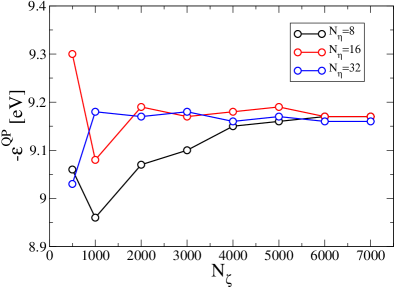
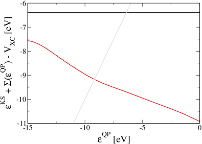
Figure 1: Left panel: Convergence of the sGW estimate of the QP hole energy for a benzene molecule as a function of $N_{\zeta}$ for different values of $N_{\eta}$. Right: A graphic representation of the self-consistent solution of Eq. (7) for $-IP=\varepsilon^{QP}$ of benzene. The solid red line represent the right hand side of Eq. (7). The intersect with the solid gray line represents the self-consistent solution. For reference, we also depict $\varepsilon^{KS}$ (solid black line).

3 Results

We now evaluate the performance of sGW by application to a set of 10 small enough molecules for which reliable deterministic calculations and experimental vertical ionization energies are available. The sGW calculation is based on the local density approximation, denoted henceforth as $\varepsilon_{\text{@LDA}}^{\text{sGW}}$ and implemented on a Fourier real-space grid using Troullier-Martins pseudopotentials ⁴⁵ and the technique for screening periodic charge images of Ref. Martyna1999. For all molecules experimental geometries were used, taken from the NIST database.⁴⁶

The sGW estimate of $\varepsilon_{\text{@LDA}}^{\text{sGW}}$ is governed by convergence of multiple parameters. The grid spacing was determined in the preparatory DFT step by requiring convergence of the LDA eigenvalues to better than 1meV (our LDA eigenvalues deviate by 0.03eV or less from those obtained by the QuantumEspresso program using the same pseudopotentials). For all molecules we chose the inverse temperature parameter as $\beta=200E_{h}^{-1}$ from which the Chebyshev expansion length $N_{C}$ was derived to be between 18,000 and 19,000 (see discussion appearing below Eq. (19)). The time propagation is performed using a discretized time-step of $\Delta t=0.05E_{h}^{-1}\hbar$ for both the Green’s function calculation as well as the RPA screening, we checked that this leads to QP energies converged to within less than 0.02eV.

Other parameters only negligibly influence the result. Specifically, the strength of the perturbation was controlled by the parameter $\tau$ (see Eq. (29)); changing its value between $0.01$ to $0.0001\;E_{h}^{-1}\hbar$ influences the QP energy by less than $0.001$eV. In practice we employ $\tau=0.001\;E_{h}^{-1}\hbar$. Furthermore, we used $N_{\xi}=100$ and ascertained that increasing this value to $200$ causes changes in the QP energies smaller than 0.01 eV.

The most influential parameters are $N_{\eta}$, the number of stochastic states $\eta$ used for the RPA screening calculation, and $N_{\zeta}$ used for representing the Green’s function. In the left panel of Fig. 1 the convergence of the QP energy for a benzene molecule is illustrated as a function of $N_{\zeta}$ for several values of $N_{\eta}$. Evidently, for this molecule, $N_{\zeta}=6000$ and $N_{\eta}=8$ are sufficient to converge the QP energy with a statistical error of $\pm 0.03\,\text{eV}$. Note that as $N_{\eta}$ increases the convergence towards the final QP value is reached after a smaller number of $N_{\zeta}$ stochastic orbitals.

When transforming from the time to the frequency domain we use a Gaussian damping factor, $\tilde{B}_{n\zeta\xi}^{r}\left(\omega\right)=\int_{0}^{T}dt\,e^{i\omega t}B_{n\zeta\xi}^{r}\left(t\right)\times e^{-\left(\gamma t\right)^{2}/2}$, where $\gamma=0.04E_{h}\hbar^{-1}$ and $T\approx 4/\gamma=100\hbar E_{h}^{-1}$ are enough to yield QP energies converged to within 0.01 eV. Note that a value of $N_{\eta}=8$ is sufficient for a stable and accurate time propagation up to $T=100\hbar E_{h}^{-1}$ but when longer times $T$ are used, $N_{\eta}$ must be increased accordingly due to an instability in stochastic TDDFT time propagation.³¹

The right panel of Fig. 1 provides a graphic representation of the self-consistent solution of Eq. (7) as the intersect between $\varepsilon^{QP}$ and $\varepsilon^{KS}+\Sigma\left(\varepsilon^{QP}\right)-V_{XC}$ . Note that even though the stochastic calculation has by its nature fluctuations, the energy dependence of $\Sigma\left(\varepsilon^{QP}\right)$ is smooth.

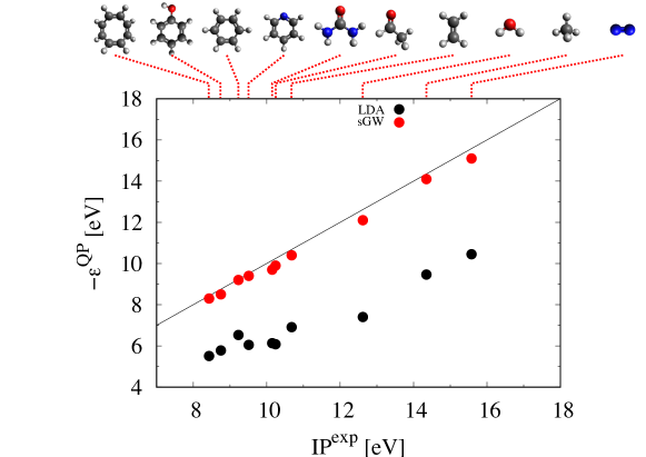
Figure 2: Ionization potentials as predicted by various calculations for the set of molecules listed in Table 1 are plotted against experimental values (note that the sGW statistical error bars are smaller than the corresponding symbol sizes). Each molecule is depicted above the graph and dotted red line points to its experimental ionization potential on the horizontal axis. The sketches of the individual molecules use black, white, blue and red spheres to indicate positions of C, H, N and O atoms respectively. LDA results that served as a starting point for the calculations are shown by black circles. $G_{0}$$W_{0}$ results are given by filled red circles. The black line represents the one-to-one correspondence to experimental values.

The sGW estimated vertical ionization energies $\varepsilon_{\text{@LDA}}^{\text{sGW}}$ were converged with respect to all parameters described above and especially, grid-size and number of stochastic orbitals $N_{\zeta}$. Hence, they should be compared to deterministic GW results which are of a complete basis set quality at the GW@LDA level, denoted $\varepsilon_{\text{@LDA}}^{\text{EXTRA}}$, extrapolated to the complete basis set limit. These results were based on the GW@PBE extrapolated results $\varepsilon_{\text{@PBE}}^{\text{EXTRA}}$ calculated under the FHI-aims code ^{34, 35} as given in Ref. 32, which were then augmented for LDA based energies using the relation:

$$\varepsilon_{\text{@LDA}}^{\text{EXTRA}}\equiv\varepsilon_{\text{@PBE}}^{\text{EXTRA}}+(\varepsilon_{\text{@LDA}}^{\text{RI}}-\varepsilon_{\text{@PBE}}^{\text{RI}}),$$ (34)

where $\varepsilon_{\text{@LDA}}^{\text{RI}}-\varepsilon_{\text{@PBE}}^{\text{RI}}$ is an estimate of the difference between PBE and LDA based GW results (typically a very small energy in the range 0.01-0.08 eV). $\varepsilon_{\text{@LDA}}^{\text{RI}}$ and $\varepsilon_{\text{@PBE}}^{\text{RI}}$ are the GW-TURBOMOLE ¹⁴ energies calculated using the def2-QZVP basis-set and the resolution-of-identity (RI) approximation. The switch between FHI-aims code and GW-TURBOMOLE codes is not expected to pose a problem since both give almost identical excitation energies ³². We have also ascertained, using several tests on small molecules, that $\varepsilon_{\text{@LDA}}^{\text{RI}}-\varepsilon_{\text{@PBE}}^{\text{RI}}$ is quite independent of the RI approximation (even though RI does affect the separate values of each energy).

System	Exp.	$\varepsilon_{\text{@PBE}}^{\text{EXTRA}}$	$\varepsilon_{\text{@LDA}}^{\text{RI}}-\varepsilon_{\text{@PBE}}^{\text{RI}}$	$\varepsilon{}_{\text{@LDA}}^{\text{EXTRA}}$	$\varepsilon_{\text{@LDA}}^{\text{sGW}}$	Diff	$h/a_{0}$	$N_{\zeta}$
benzene	9.23	9.10(0.01)	0.03	9.13	9.17(0.03)	0.04	0.30	6000
cyclooctatetraene	8.43	8.18(0.02)	0.02	8.20	8.33(0.03)	0.13	0.35	6000
acetaldehyde	10.20	9.66(0.03)	0.08	9.74	9.90(0.06)	0.16	0.30	8000
water	12.60	12.05(0.03)	0.08	12.13	12.10(0.02)	-0.04	0.25	8000
phenol	8.75	8.51(0.01)	0.05	8.56	8.61(0.03)	0.05	0.35	9000
urea	10.15	9.46(0.02)	0.12	9.58	9.65(0.05)	0.07	0.30	11000
methane	14.40	14.00(0.06)	0.03	14.03	14.09(0.01)	0.06	0.40	10000
nitrogen	15.60	15.05(0.04)	0.11	15.16	15.05(0.06)	-0.11	0.35	7000
ethylene	10.70	10.40(0.03)	0.03	10.43	10.40(0.06)	-0.03	0.35	12000
pyridine	9.50	9.17(0.01)	0.06	9.23	9.42(0.04)	0.19	0.35	7000
					Mean:	0.05
					Mean Abs:	0.09

Table 1: Vertical ionization energies (eV) for the indicated molecules. The complete-basis-set-limit-extrapolated GW@PBE result, $\varepsilon_{\text{@PBE}}^{\text{EXTRA}}$ (with extrapolation uncertainties in parenthesis) is taken from Ref. 32. $\varepsilon_{\text{@LDA}}^{\text{RI}}-\varepsilon_{\text{@PBE}}^{\text{RI}}$is the estimated GW@LDA to GW@PBE difference, calculated using GW-TURBOMOLE ¹⁴ within the RI approximation and the def2-QZVP basis-set. The extrapolated GW@LDA results $\varepsilon{}_{\text{@LDA}}^{\text{EXTRA}}$ represent our estimate of the fully converged GW@LDA energies (given in Eq. 34) which are used to benchmark the sGW@LDA energies $\varepsilon{}_{\text{@LDA}}^{\text{sGW}}$ (with statistical uncertainties given in parenthesis). For each molecule, the grid spacing $h$ and the number of stochastic orbitals $N_{\zeta}$ required for producing converged sGW to the indicated accuracy are given in the table.

In Table 1 we compare the GW and sGW LDA-based vertical ionization energies, showing a high level of agreement, with mean and absolute deviations of $0.05\,\text{eV}$ and $0.09$eV respectively, typically of the order of the given uncertainties in the deterministic and the stochastic calculations.

We also note that both these values are also in good overall agreement with experimental values, as seen in Fig. 2, although both results (stochastic or deterministic) generally underestimate the experiment by 0.1-0.5 eV. This is primarily due to the known limitations of the $\text{G}_{0}\text{W}_{0}$ approach, which can be improved using self consistent-GW.^{6, 13, 17, 47}

4 Conclusions

In conclusion, we reviewed in detail the sGW method and its algorithmic implementation. The sGW exhibits a near-linear scaling with system size complexity ³⁰ and hence for large systems it is expected to be much faster relative to the deterministic basis-set implementations having quartic or quintic ¹⁴ asymptotic scaling. Therefore, comparison of sGW estimations with those of deterministic GW can only be made on relatively small molecules and here we selected a set of 10 such molecules having $N_{e}=10-50$ electrons. For this set, the execution time of sGW was larger than that of deterministic GW codes and we estimate that the crossover would occur for molecules with $N_{e}\approx 200$. For the selected set of molecules, sGW and deterministic GW predicted vertical ionization energies which were very close, with maximal deviation smaller than 0.2 eV and average and absolute deviations of 0.05eV and 0.1eV. This work was supported by the Israel Science Foundation – FIRST Program (Grant No. 1700/14) and the Center for Computational Study of Excited-State Phenomena in Energy Materials at the Lawrence Berkeley National Laboratory, which is funded by the U.S. Department of Energy, Office of Science, Basic Energy Sciences, Materials Sciences and Engineering Division under Contract No. DE-AC02-05CH11231, as part of the Computational Materials Sciences Program. Some of the calculations were performed as part of the XSEDE computational project TG-CHE160092.

References

- Hohenberg and Kohn 1964 Hohenberg, P.; Kohn, W. Inhomogeneous Electron Gas. Phys. Rev. 1964, 136, B864
- Kohn and Sham 1965 Kohn, W.; Sham, L. J. Self-Consistent Equations Including Exchange and Correlation Effects. Phys. Rev. 1965, 140, A1133
- VandeVondele et al. 2012 VandeVondele, J.; Borstnik, U.; Hutter, J. r. Linear scaling self-consistent field calculations with millions of atoms in the condensed phase. J. Chem. Theory Comput. 2012, 8, 3565–3573
- Hybertsen and Louie 1985 Hybertsen, M. S.; Louie, S. G. First-principles theory of quasiparticles: calculation of band gaps in semiconductors and insulators. Phys. Rev. Lett. 1985, 55, 1418
- Steinbeck et al. 1999 Steinbeck, L.; Rubio, A.; Reining, L.; Torrent, M.; White, I.; Godby, R. Enhancements to the GW space-time method. Comput. Phys. Commun. 1999, 125, 05–118
- Shishkin and Kresse 2007 Shishkin, M.; Kresse, G. Self-consistent GW calculations for semiconductors and insulators. Phys. Rev. B 2007, 75, 235102
- Rostgaard et al. 2010 Rostgaard, C.; Jacobsen, K. W.; Thygesen, K. S. Fully self-consistent GW calculations for molecules. Phys. Rev. B 2010, 81, 085103
- Foerster et al. 2011 Foerster, D.; Koval, P.; Sánchez-Portal, D. An O (N3) implementation of Hedin’s GW approximation for molecules. J. Chem. Phys. 2011, 135, 074105
- Faber et al. 2011 Faber, C.; Attaccalite, C.; Olevano, V.; Runge, E.; Blase, X. First-principles GW calculations for DNA and RNA nucleobases. Phys. Rev. B 2011, 83, 115123
- Blase et al. 2011 Blase, X.; Attaccalite, C.; Olevano, V. First-principles GW calculations for fullerenes, porphyrins, phtalocyanine, and other molecules of interest for organic photovoltaic applications. Phys. Rev. B 2011, 83, 115103
- Deslippe et al. 2012 Deslippe, J.; Samsonidze, G.; Strubbe, D. A.; Jain, M.; Cohen, M. L.; Louie, S. G. BerkeleyGW: A massively parallel computer package for the calculation of the quasiparticle and optical properties of materials and nanostructures. Comput. Phys. Commun. 2012, 183, 1269 – 1289
- Marom et al. 2012 Marom, N.; Caruso, F.; Ren, X.; Hofmann, O. T.; Körzdörfer, T.; Chelikowsky, J. R.; Rubio, A.; Scheffler, M.; Rinke, P. Benchmark of GW methods for azabenzenes. Phys. Rev. B 2012, 86, 245127
- Caruso et al. 2012 Caruso, F.; Rinke, P.; Ren, X.; Scheffler, M.; Rubio, A. Unified description of ground and excited states of finite systems: The self-consistent GW approach. Phys. Rev. B 2012, 86, 081102
- van Setten et al. 2013 van Setten, M.; Weigend, F.; Evers, F. The GW-Method for Quantum Chemistry Applications: Theory and Implementation. J. Chem. Theory Comput. 2013, 9, 232–246
- Pham et al. 2013 Pham, T. A.; Nguyen, H.-V.; Rocca, D.; Galli, G. GW calculations using the spectral decomposition of the dielectric matrix: Verification, validation, and comparison of methods. Phys. Rev. B 2013, 87, 155148
- Govoni and Galli 2015 Govoni, M.; Galli, G. Large scale GW calculations. Journal of chemical theory and computation 2015, 11, 2680–2696
- Kaplan et al. 2016 Kaplan, F.; Harding, M. E.; Seiler, C.; Weigend, F.; Evers, F.; van Setten, M. J. Quasi-Particle Self-Consistent GW for Molecules. J. Chem. Theory Comput. 2016,
- Heyd et al. 2003 Heyd, J.; Scuseria, G. E.; Ernzerhof, M. Hybrid functionals based on a screened Coulomb potential. J. Chem. Phys. 2003, 118, 8207–8215
- Baer et al. 2010 Baer, R.; Livshits, E.; Salzner, U. Tuned Range-separated hybrids in density functional theory. Annu. Rev. Phys. Chem. 2010, 61, 85–109
- Kronik et al. 2012 Kronik, L.; Stein, T.; Refaely-Abramson, S.; Baer, R. Excitation Gaps of Finite-Sized Systems from Optimally Tuned Range-Separated Hybrid Functionals. J. Chem. Theory Comput. 2012, 8, 1515–1531
- Neuhauser et al. 2015 Neuhauser, D.; Rabani, E.; Cytter, Y.; Baer, R. Stochastic Optimally Tuned Range-Separated Hybrid Density Functional Theory. J. Phys. Chem. A 2015, 120, 3071–3078
- Hedin 1965 Hedin, L. New Method for Calculating the One-Particle Green’s Function with Application to the Electron-Gas Problem. Phys. Rev. 1965, 139, A796–A823
- Hybertsen and Louie 1986 Hybertsen, M. S.; Louie, S. G. Electron correlation in semiconductors and insulators: Band gaps and quasiparticle energies. Phys. Rev. B 1986, 34, 5390–5413
- Aryasetiawan and Gunnarsson 1998 Aryasetiawan, F.; Gunnarsson, O. The GW method. Rep. Prog. Phys. 1998, 61, 237–312
- Onida et al. 2002 Onida, G.; Reining, L.; Rubio, A. Electronic excitations: density-functional versus many-body Green’s-function approaches. Rev. Mod. Phys. 2002, 74, 601–659
- Friedrich and Schindlmayr 2006 Friedrich, C.; Schindlmayr, A. Many-body perturbation theory: the GW approximation. NIC Series 2006, 31, 335
- Rohlfing and Louie 2000 Rohlfing, M.; Louie, S. G. Electron-hole excitations and optical spectra from first principles. Phys. Rev. B 2000, 62, 4927–4944
- Benedict et al. 2003 Benedict, L. X.; Puzder, A.; Williamson, A. J.; Grossman, J. C.; Galli, G.; Klepeis, J. E.; Raty, J.-Y.; Pankratov, O. Calculation of optical absorption spectra of hydrogenated Si clusters: Bethe-Salpeter equation versus time-dependent local-density approximation. Phys. Rev. B 2003, 68, 085310
- Tiago and Chelikowsky 2006 Tiago, M. L.; Chelikowsky, J. R. Optical excitations in organic molecules, clusters, and defects studied by first-principles Green function methods. Phys. Rev. B 2006, 73, 205334
- Neuhauser et al. 2014 Neuhauser, D.; Gao, Y.; Arntsen, C.; Karshenas, C.; Rabani, E.; Baer, R. Breaking the Theoretical Scaling Limit for Predicting Quasiparticle Energies: The Stochastic G W Approach. Phys. Rev. Lett. 2014, 113, 076402
- Rabani et al. 2015 Rabani, E.; Baer, R.; Neuhauser, D. Time-dependent stochastic Bethe-Salpeter approach. Phys. Rev. B 2015, 91, 235302
- van Setten et al. 2015 van Setten, M. J.; Caruso, F.; Sharifzadeh, S.; Ren, X.; Scheffler, M.; Liu, F.; Lischner, J.; Lin, L.; Deslippe, J. R.; Louie, S. G.; Yang, C.; Weigend, F.; Neaton, J. B.; Evers, F.; Rinke, P. GW 100: Benchmarking G 0 W 0 for Molecular Systems. J. Chem. Theory Comput. 2015, 11, 5665–5687
- Furche et al. 2014 Furche, F.; Ahlrichs, R.; Hättig, C.; Klopper, W.; Sierka, M.; Weigend, F. Turbomole. Wiley Interdisciplinary Reviews: Computational Molecular Science 2014, 4, 91–100
- Blum et al. 2009 Blum, V.; Gehrke, R.; Hanke, F.; Havu, P.; Havu, V.; Ren, X.; Reuter, K.; Scheffler, M. Ab initio molecular simulations with numeric atom-centered orbitals. Computer Physics Communications 2009, 180, 2175–2196
- Ren et al. 2012 Ren, X.; Rinke, P.; Blum, V.; Wieferink, J.; Tkatchenko, A.; Sanfilippo, A.; Reuter, K.; Scheffler, M. Resolution-of-identity approach to Hartree–Fock, hybrid density functionals, RPA, MP2 and GW with numeric atom-centered orbital basis functions. New Journal of Physics 2012, 14, 053020
- Nguyen et al. 2012 Nguyen, H.-V.; Pham, T. A.; Rocca, D.; Galli, G. Improving accuracy and efficiency of calculations of photoemission spectra within the many-body perturbation theory. Phys. Rev. B 2012, 85, 081101
- Baer et al. 2013 Baer, R.; Neuhauser, D.; Rabani, E. Self-Averaging Stochastic Kohn-Sham Density-Functional Theory. Phys. Rev. Lett. 2013, 111, 106402
- Neuhauser et al. 2014 Neuhauser, D.; Baer, R.; Rabani, E. Communication: Embedded fragment stochastic density functional theory. J. Chem. Phys. 2014, 141, 041102
- Hutchinson 1990 Hutchinson, M. F. A stochastic estimator of the trace of the influence matrix for Laplacian smoothing splines. Communications in Statistics-Simulation and Computation 1990, 19, 433–450
- Baer and Head-Gordon 1997 Baer, R.; Head-Gordon, M. Chebyshev expansion methods for electronic structure calculations on large molecular systems. J. Chem. Phys. 1997, 107, 10003–10013
- Baer and Head-Gordon 1997 Baer, R.; Head-Gordon, M. Sparsity of the density matrix in Kohn-Sham density functional theory and an assessment of linear system-size scaling methods. Phys. Rev. Lett. 1997, 79, 3962–3965
- Baer and Neuhauser 2004 Baer, R.; Neuhauser, D. Real-time linear response for time-dependent density-functional theory. J. Chem. Phys. 2004, 121, 9803–9807
- Fetter and Walecka 1971 Fetter, A. L.; Walecka, J. D. Quantum Thoery of Many Particle Systems; McGraw-Hill: New York, 1971; p 299
- Gao et al. 2015 Gao, Y.; Neuhauser, D.; Baer, R.; Rabani, E. Sublinear scaling for time-dependent stochastic density functional theory. J. Chem. Phys. 2015, 142, 034106
- Troullier and Martins 1991 Troullier, N.; Martins, J. L. Efficient Pseudopotentials for Plane-Wave Calculations. Phys. Rev. B 1991, 43, 1993–2006
- 46 NIST Computational Chemistry Comparison and Benchmark Database NIST Standard Reference Database Number 101 Release 18, October 2016, Editor: Russell D. Johnson III http://cccbdb.nist.gov/,
- Vlček et al. 2017 Vlček, V.; Baer, R.; Rabani, E.; Neuhauser, D. Self-consistent band-gap renormalization GW. arXiv preprint arXiv:1701.02023 2017,