Realistic Injection Simulations of a Cyclotron Spiral Inflector using OPAL

Abstract

We present an upgrade to the particle-in-cell ion beam simulation code OPAL that enables us to run highly realistic simulations of the spiral inflector system of a compact cyclotron. This upgrade includes a new geometry class and field solver that can handle the complicated boundary conditions posed by the electrode system in the central region of the cyclotron both in terms of particle termination, and calculation of self-fields. Results are benchmarked against the analytical solution of a coasting beam. As a practical example, the spiral inflector and the first revolution in a 1 MeV/amu test cyclotron, located at Best Cyclotron Systems, Inc., are modeled and compared to the simulation results. We find that OPAL can now handle arbitrary boundary geometries with relative ease. Comparison of simulated injection efficiencies, and beam shape compare well with measured efficiencies and a preliminary measurement of the beam distribution after injection.

I Introduction

OPAL Adelmann et al. (2016) is a particle-in-cell (PIC) code developed for the simulation of particle accelerators. It is highly parallel and comes in two distinct flavors: OPAL-cycl (specific to cyclotrons and rings) and OPAL-t (general purpose). For the presented application, we focus on OPAL-cycl   which has been used very successfully to simulate existing high intensity cyclotrons like the PSI Injector II Yang et al. (2010), and PSI Ring Cyclotron Yang et al. (2010); Bi et al. (2011) as well as to design new cyclotrons like CYCIAE Zhang et al. (2012), DAE$\delta$ALUS Abs et al. (2012); Aberle et al. (2013), and IsoDAR Adelmann et al. (2012); Bungau et al. (2012).

However, one piece has been missing so far: the axial injection using a spiral inflector or an electrostatic mirror. Both are electrostatic devices that bend the beam from the axial direction into the mid-plane of the cyclotron where it is subsequently accelerated. A schematic view of this type of injection for a spiral inflector is shown in Figure 1.

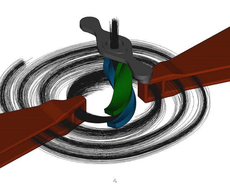
Figure 1: Schematic of a spiral inflector with particle trajectories from an OPAL simulation. The beam enters axially (from the top) through an aperture (grey) and is bent into the mid-plane by a combination of the electrostatic field generated by the spiral electrodes (green and blue, voltage typically symmetric at $+\mathrm{V}_{\textrm{spiral}}$ and $-\mathrm{V}_{\textrm{spiral}}$) and the cyclotron’s main magnetic field. Then it is accelerated by the two Dees (copper, Dummy-Dees not shown). Color online.

In order to enable OPAL-cycl to track particles through a complicated set of electrodes like a spiral inflector, the following additions have been made:

• The Smooth Aggregation Algebraic Multi Grid (SAAMG) solver Adelmann et al. (2010) has been extended to include arbitrarily shaped boundaries.

• A geometry class has been implemented that provides boundary conditions to the field solver and handles particle termination should their trajectories intersect with the electrodes.

• A number of improvements have been made to the internal coordinate transformations and the handling of beam rotations in OPAL-cycl in order to accommodate the injection off-mid-plane.

These additions will be discussed in Section II and references therein. At the end of this section, a benchmark against the analytical solution of a coasting beam in a grounded beam pipe with variable axial offset will be presented.

A specific example of the usefulness of realistic spiral inflector simulations is the ongoing R&D effort for the DAE$\delta$ALUS Abs et al. (2012); Aberle et al. (2013), and IsoDAR Adelmann et al. (2012); Bungau et al. (2012) experiments (described briefly in Section III). In both cases, a very high intensity beam ($\approx 10-30$ mA average) needs to be injected, which is higher than current state-of-the-art cyclotrons have demonstrated. Part of the R&D for these projects was an experiment in collaboration with Best Cyclotron Systems, Inc. (BCS) in Vancouver, Canada to test a flat-field ECR ion source, transport through the Low Energy Beam Transport System (LEBT) and finally injection into a small test cyclotron through a spiral inflector. The results of this campaign are described in much detail in Alonso et al. (2015) and the most important points will be reiterated in Section III, before OPAL simulation results are bench-marked against the experimental results.

II The particle-in-cell code OPAL

For this discussion we briefly introduce OPAL-cycl Yang et al. (2010), one of the four flavours of OPAL.

II.1 Governing equation

The collision between particles can be neglected in the cyclotron under consideration, because the typical bunch densities are low. The general equations of motion of charged particles in electromagnetic fields can be expressed in time domain by

$$\frac{d\mathbf{p}(t)}{dt}=q\left(c\mbox{\boldmath$\beta$}\times\mathbf{B}+\mathbf{E}\right),\\$$

where $m_{0},q,\gamma$ are rest mass, charge and the relativistic factor. With $\mathbf{p}=m_{0}c\gamma\mbox{\boldmath$\beta$}$ we denote the momentum of a particle, $c$ is the speed of light, and $\mbox{\boldmath$\beta$}=(\beta_{x},\beta_{y},\beta_{z})$ is the normalized velocity vector. The time ($t$) and position ($\mathbf{x}$) dependent electric and magnetic vector fields are written in abbreviated form as $\mathbf{E}$ and $\mathbf{B}$.

If $\mathbf{p}$ is normalized by $m_{0}c$, Eq. (II.1) can be rewritten component wise in Cartesian coordinates as

$$\frac{dp_{x}}{dt} = \frac{q}{m_{0}c}E_{x}+\frac{q}{\gamma m_{0}}(p_{y}B_{z}-p_{z}B_{y}),$$

$$\frac{dp_{y}}{dt} = \frac{q}{m_{0}c}E_{y}+\frac{q}{\gamma m_{0}}(p_{z}B_{x}-p_{x}B_{z}),$$ (1)

$$\frac{dp_{z}}{dt} = \frac{q}{m_{0}c}E_{z}+\frac{q}{\gamma m_{0}}(p_{x}B_{y}-p_{y}B_{x}).$$

The evolution of the beam’s distribution function

$$f(\mathbf{x},c\mbox{\boldmath$\beta$},t):(\Re^{M}\times\Re^{M}\times\Re)\rightarrow\Re$$

can be expressed by a collisionless Vlasov equation:

$$\frac{df}{dt}=\partial_{t}f+c\mbox{\boldmath$\beta$}\cdot\nabla_{x}f+q(\mathbf{E}+c\mbox{\boldmath$\beta$}\times\mathbf{B})\cdot\nabla_{c\mbox{\boldmath$\beta$}}f=0.$$ (2)

Here we have assumed that $M$ particles of the same species are within the beam. In this particular case, $\mathbf{E}$ and $\mathbf{B}$ include both external applied fields and space charge fields, all other fields are neglected.

$$\mathbf{E} = \mathbf{E}_{\mathrm{ext}}+\mathbf{E}_{\mathrm{sc}},$$

$$\mathbf{B} = \mathbf{B}_{\mathrm{ext}}+\mathbf{B}_{\mathrm{sc}}.$$ (3)

II.2 Bunch rotations

In OPAL-cycl, the coordinate system is different from OPAL-t: The x and y coordinates are the horizontal coordinates (the cyclotron mid-plane) and z is the vertical coordinate. Internally, both Cartesian (x, y, z) and cylindrical (r, $\Theta$, z) coordinate systems are used. For simplicity, in the past, the injection of bunches in OPAL-cycl had to happen on the cyclotron mid-plane with the option to include an offset in z direction within the particle distribution itself. The global coordinates of the beam centroid were thus restricted to r and $\Theta$. In order to accommodate the injection of a bunch far away from the mid-plane and a mean momentum aligned with the z-axis, the handling of rotations in OPAL-cycl was updated from 2D rotations in the mid-plane to arbitrary rotations/translations in three-dimensional (3D) space. Quaternions Hamilton (1844) were chosen to avoid gimbal-lock Mitchell and Rogers (1965) and a set of rotation functions was implemented. These are now used throughout OPAL-cycl. Outside of the new SPIRAL mode, quaternions are also used to align the mean momentum of the bunch with the y axis before solving for self-fields in order to simplify the inclusion of relativistic effects in the calculation of self-fields. In the SPIRAL mode, no relativistic effects are taken into account due to the low injection energy (typically $<100$ keV).

II.3 Fieldsolver

The space charge fields can be obtained by a quasi-static approximation. In this approach, the relative motion of the particles is non-relativistic in the beam rest frame, so the self-induced magnetic field is practically absent and the electric field can be computed by solving Poisson’s equation

$$\nabla^{2}\phi(\mathbf{x})=-\frac{\rho(\mathbf{x})}{\varepsilon_{0}},$$ (4)

where $\phi$ and $\rho$ are the electrostatic potential and the spatial charge density in the beam rest frame. The electric field can then be calculated by

$$\mathbf{E}_{\mathrm{sc}}=-\nabla\phi,$$ (5)

and back transformed to yield both the electric and the magnetic fields, in the lab frame, required in Eq. (II.1) by means of a Lorentz transformation. As mentioned in the previous section, this step is omitted in the SPIRAL mode of OPAL-cycl by setting $\gamma=1$.

A parallel 3D Poisson solver for the electrostatic potential computation in a round beam pipe geometry with open-end boundary conditions is presented in  Adelmann et al. (2010).

In this section, we present a method for solving the space charge Poisson problem (6) in much more complex geometries of particle accelerators. The problem discretization takes into account the complex geometries of beam pipe elements and the space charge forces are computed within the geometry. This assures that the space charge components are taken properly into account in any type of geometry.

$$-\Delta\phi =\frac{\rho}{\epsilon_{0}}\ \text{in}\ \Omega,$$ (6)

$$\phi =g\equiv 0\ \text{on}\ \partial\Omega$$

where $\Omega$ represents the computational domain, and $\partial\Omega$ the boundary surface of the geometry. Our approach solving the Poisson problem in complex geometries includes the unstructured and structured meshes. Unstructured meshes are used to define the complex geometry because they are easy to conform a block to a complicated shape, and structured meshes are used for the finite-difference discretization method.

II.3.1 Spatial discretization

To solve the Poisson problem (6) on $\Omega$, we use a cell-centered discretization for Laplacian. A grid point is called interior if all its neighbors are in $\Omega$, or near-boundary point otherwise. The discrete Laplacian with mesh spacing $h$ on interior points is defined as the regular seven-point finite difference approximation of $-\Delta$.

$$L{\hat{\phi}}(\mathbf{x})=\sum_{i=1}^{3}\frac{-{\hat{\phi}}(\mathbf{x}-h\mathbf{e}_{i})+2{\hat{\phi}}(\mathbf{x})-{\hat{\phi}}(\mathbf{x}+h\mathbf{e}_{i})}{h^{2}},$$ (7)

where $\mathbf{e}_{i}$ is the $i$th coordinate vector Forsythe and Wasow (1960).

At near-boundary point, $\mathbf{x}$ in Figure 2 where not all its neighbors are in the domain, we use an approximation for Laplacian and the value of $\hat{\phi}$ at near-boundary point is obtained by one of the extrapolation method described in Adelmann et al. (2010). The approximation is based on linear extrapolation of near-boundary points ($0<s\leq 1$):

$$L{\hat{\phi}}(\mathbf{x})=\sum_{i=1}^{3}-\frac{1}{sh}{\hat{\phi}}(\mathbf{x}_{L})+\frac{1}{h}\left(\frac{1}{s}+\frac{1}{h}\right){\hat{\phi}}(\mathbf{x})-\frac{1}{h^{2}}{\hat{\phi}}(\mathbf{x}_{R}),$$ (8)

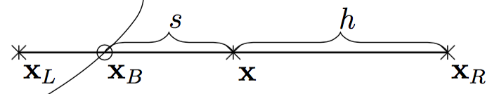
Figure 2: $\mathbf{x}_{L}=\mathbf{x}-h\mathbf{e}_{i}$, $\mathbf{x}_{B}=\mathbf{x}-sh\mathbf{e}_{i}$, $\mathbf{x}$ and $\mathbf{x}_{R}=\mathbf{x}+h\mathbf{e}_{i}$ are the point outside of $\Omega$, boundary point, near-boundary point and interior point.

The value of ${\hat{\phi}}$ at $\mathbf{x}_{L}$ is defined through one of the extrapolation method in Eq. (9).

$$\rm{Constant:}\ {\hat{\phi}}(\mathbf{x}_{L}) =g(\mathbf{x}_{B})$$ (9)

$$\rm{Linear:}\ {\hat{\phi}}(\mathbf{x}_{L}) =\left(1-\frac{1}{s}\right){\hat{\phi}}(\mathbf{x})+\frac{1}{s}g(\mathbf{x}_{B})$$

II.3.2 Implementation

The query class, an interface to search for the points inside of the irregular domain is implemented. Once the points inside the irregular domain are detected, their intersection values in six different directions are stored in containers. The coordinates values are mapped into its intersection values to be used as a fast look-up table. The distances between the near-boundary point and its intersection values are used for the linear extrapolation.

The finite difference approximation of the Poisson problem requires solving a system of linear equations to compute the electrostatic potential. The resulting linear system is solved using the preconditioned conjugate gradient algorithm complemented by an algebraic multigrid preconditioner using the Trilinos framework Heroux et al. (2005). Trilinos is a collection of software packages that support parallel linear algebra computations on distributed memory architectures, in particular the solution of linear systems of equations. Epetra provides the data structures that are needed in the linear algebra libraries. Amesos, AztecOO, and Belos are packages providing direct and iterative solvers. ML is the multi-level package, that constructs and applies the smoothed aggregation-based multigrid preconditioners.

II.4 External fields

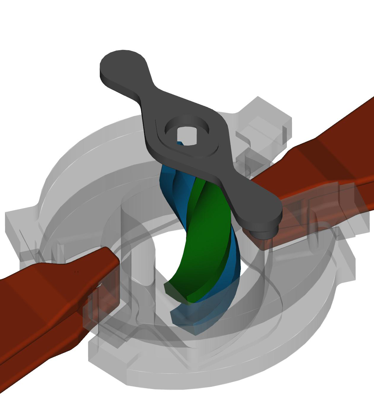
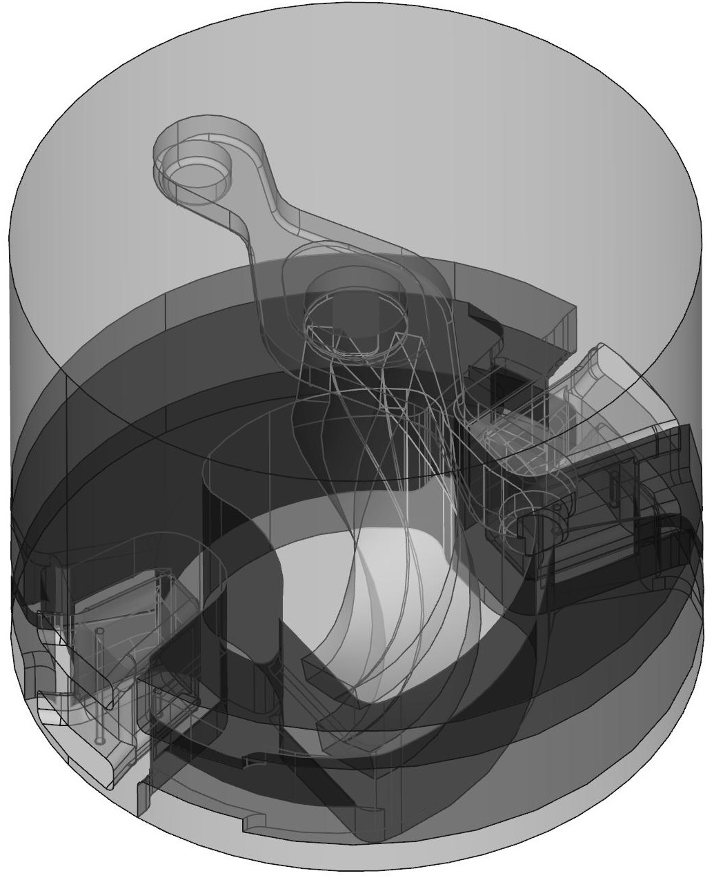
(a) CAD Model	(b) Inverted
(c) Meshed	(d) Voxels

Figure 3: The four stages of OPAL geometry preparation: (a) Initial CAD model of the electrodes in the system. (b) An inverted solid is created by subtraction of all elements in (a) from a “master volume” (in this case a cylindrical outer chamber). (c) The inverted geometry is saved in stp format and a mesh is generated using GMSH Geuzaine and Remacle (2009). (d) During the initialization phase, OPAL creates a voxel mesh to speed up the tests that have to be performed every time-step (cf. text).

With respect to the external magnetic field two possible situations can be considered: in the first situation, the real field map is available on the median plane of the existing cyclotron machine using measurement equipment. In most cases concerning cyclotrons, the vertical field, $B_{z}$, is measured on the median plane ($z=0$) only. Since the magnetic field outside the median plane is required to compute trajectories with $z\neq 0$, the field needs to be expanded in the $Z$ direction. According to the approach given by Gordon and Taivassalo Gordon and Taivassalo (1985), by using a magnetic potential and measured $B_{z}$ on the median plane at the point $(r,\theta,z)$ in cylindrical polar coordinates, the 3$rd$ order field can be written as

$$\vec{B}_{\mathrm{ext}}(r,\theta,z)=\begin{pmatrix}z\frac{\partial B_{z}}{\partial r}-\frac{1}{6}z^{3}C_{r}\\ \frac{z}{r}\frac{\partial B_{z}}{\partial\theta}-\frac{1}{6}\frac{z^{3}}{r}C_{\theta}\\ B_{z}-\frac{1}{2}z^{2}C_{z}\end{pmatrix}$$ (10)

where $B_{z}\equiv B_{z}(r,\theta,0)$ and

$$C_{r} = \frac{\partial^{3}B_{z}}{\partial r^{3}}+\frac{1}{r}\frac{\partial^{2}B_{z}}{\partial r^{2}}-\frac{1}{r^{2}}\frac{\partial B_{z}}{\partial r}+\frac{1}{r^{2}}\frac{\partial^{3}B_{z}}{\partial r\partial\theta^{2}}-\frac{2}{r^{3}}\frac{\partial^{2}B_{z}}{\partial\theta^{2}},$$

$$C_{\theta} = \frac{1}{r}\frac{\partial^{2}B_{z}}{\partial r\partial\theta}+\frac{\partial^{3}B_{z}}{\partial r^{2}\partial\theta}+\frac{1}{r^{2}}\frac{\partial^{3}B_{z}}{\partial\theta^{3}},$$ (11)

$$C_{z} = \frac{1}{r}\frac{\partial B_{z}}{\partial r}+\frac{\partial^{2}B_{z}}{\partial r^{2}}+\frac{1}{r^{2}}\frac{\partial^{2}B_{z}}{\partial\theta^{2}}.$$

All the partial differential coefficients are computed on the median plane data by interpolation, using Lagrange’s 5-point formula. In the other situation, the 3D field for the region of interest is calculated numerically by building a 3D model using commercial software during the design phase of a new cyclotron. In this case the calculated field will be more accurate, especially at large distances from the median plane, i.e. a full 3D field map can be calculated. For all calculations in this paper, we use the second method. Fields (where applicable) are generated as 3D field maps with VectorFields OPERA OPERA3D (2013). In case of RF fields, OPAL-cycl varies the field with a cosine function:

$$\vec{E}_{\mathrm{OPAL}}(t)=\vec{E}_{\mathrm{OPERA}}\cdot\cos(\omega_{\mathrm{rf}}t-\phi_{S})$$ (12)

where $t$ is the time of flight, $\omega_{\mathrm{rf}}$ the RF frequency, and $\phi_{S}$ the starting phase of the particle.

Finally, in this paper, both the external fields and self-fields are used to track particles during each time step using a 4^th order Runge-Kutta (RK) integrator, in which the fields are evaluated four times in each time step. Space charge fields are assumed to be constant during one time step, because their variation is typically much slower than that of external fields.

II.5 Geometry

For the simulation of precise beam dynamics, an exact modelling of the accelerator geometry is essential. Usually a CAD model of the accelerator or part of it is already available (Figure 3(a)). From these models we need to create the vacuum chamber or beam-pipe for specifying the boundary, i.e. the simulation domain ($\Omega$ in Eq. 6). In case of the spiral inflector, we have to add a cylinder to limit the vacuum chamber (figure Figure 3(b)). This modified CAD model can be used to create a triangle mesh $T$ modeling the vacuum chamber of the inflector (Figure 3(c)).

Facilitating a meshed vacuum chamber or beam-pipe, OPAL is able to model arbitrary accelerator geometries and provides methods for

1. testing whether a particle will collide with the inner surface of the geometry (boundary, $\partial\Omega$) in the next time step

2. computing the distance $d=|x_{0}-I|$ from a given point $x_{0}$ to the boundary intersection point $I$ with $\partial\Omega$ (c.f. Figure 4)

3. testing whether a given point $x_{0}$ is inside the geometry. Only points inside the geometry are in the computational domain $\Omega$.

The geometry can consist of multiple parts. Each part must be modeled as a 3D closed volume. The used methods are based on well known methods in computer graphics, especially ray tracing Sunday .

II.5.1 Initializing the geometry

For testing whether a particle will collide with the boundary in then next time step, we can run a line segment/triangle intersection test for all triangles in the mesh. Even to be able to model simple structures, triangle meshes with thousands of elements are required. Applying a brute force algorithm, we have to run this test for all particles per time-step, rendering the naive approach as not feasible due to performance reasons.

In computer graphics this problem is efficiently solved by using voxel meshes. A voxel is a volume pixel representing a value on a regular 3D grid. Voxel meshes are used to render and model 3D objects.

To reduce the number of required line segment – triangle intersection tests, a voxel mesh $V$ covering the triangle mesh $T$ is created during initialization of OPAL. In this step, all triangles are assigned to their intersecting voxels. Whereby a triangle usually intersects with more than one voxel.

For the line segment/triangle intersection tests we can now reduce the required tests to the triangles assigned to the voxels intersecting the line segment. The particle boundary collision test can be improved further by comparing the particle momentum and the inward pointing normal $\vec{n}$ of the triangles.

In the following, we use the following definitions:

$T$

represents the set of triangles in the triangulated mesh.

$V$

represents the set of voxels modelling the voxelized triangle mesh.

$L$

a closed line segment bounded by points $x_{0}$ and $x_{1}$ (c.f. figure Figure 4).

$R$

a ray defined by the starting point $x_{0}$ passing through $x_{1}$.

$T_{v}\subset T$

represents the subset of triangles $t\in T$ which have intersections with $v\in V$.

$V_{L}\subset V$

represents the subset of voxels $v\in V$ which intersections with the line segment $L$.

$I_{t,L}$

represents an intersection point of a line segment $L$ with a triangle $t\in T$.

$T_{L}$

represents the set of tuples $(t_{L},I_{t,L})$ with $t_{L}\in T$ intersects with $L$.

II.5.2 Basic ray/line-segment boundary intersection test

In the first step, we have to compute $V_{L}$, which is the set of voxels in the voxel mesh $V$ which have intersections with the given line-segment or ray $L$. With

$$T_{v}=\{t\in T\,|\,t\,\textrm{\it intersects with }v\}$$

we can compute a small subset of triangles

$$T_{V,L}=\{\cup T_{v},\forall\,v\in V_{L}\}$$

which might have intersections with $L$. We have to run the ray/line-segment triangle test only for all triangles in $T_{V,L}$.

Figure 4: The boundary $\partial\Omega$ is discretized by a set of triangles $T$. Shown is the line $(x_{0},x_{1})$ triangle $t\in T$ intersection test, with intersection at $\mathbf{I}\in\partial\Omega$.

(85, 55)[basicIntersectionTest(L)] $V_{L}=\{v\in V\,|\,v\,\textrm{\it intersects with }L\}$ $T_{V,L}=\{t\in T\,|\,t\,\textrm{\it intersects with a voxel }v\in V_{L}\}$ $T_{L}=\{\}$ // result $\textrm{\it for each}\,t\in T_{V,L}$

II.6 Simple Test Case

Figure 5: Cross-sectional view of beam off-centered by $\xi$ along the x-axis. A mirror line charge of $-\rho_{L}$ is also depicted at $\frac{r_{p}^{2}}{\xi}$. Adapted from (Reiser, 2008, p229).

In order to test the proper functionality of the SAAMG fieldsolver in combination with an external geometry file, we compared the calculated fields and potentials of a FLATTOP distribution (uniformly populated cylinder) inside a geometry generated according to the previous subsection with the analytical solution of a uniformly charged cylindrical beam inside a conducting pipe. The geometry file we used contained a 1 m long beam pipe with 0.1 m radius. For a concentric beam, a regular Fast Fourier Transform (FFT) field solver is sufficient. However, if the beam is off-centered by an amount $\xi$ (see Figure 5) and especially, when it is close to the conducting walls of the beam pipe, the electric field calculated by the FFT solver does no longer reproduce reality. This is even more true for complicated geometries like a spiral inflector. To compare the simulated results with the analytical solution presented below, all simulations were run in such a way that the bunch frequency $f_{b}$ was adjusted such that for a given bunch length $l_{b}$ and beam velocity $v_{b}$ the given beam current $I$ corresponded to the equivalent DC beam current (i.e. subsequent bunches are head-to-tail):

$$f_{b}=\frac{v_{b}}{l_{b}}$$ (13)

The bunch radius $r_{b}$ was chosen to be 0.01 m and the length $l_{b}$ to be 0.6 m so that in the center of the bunch to very good approximation the conditions of an infinitely long beam hold.

Figure 6: $\chi^{2}_{\mathrm{red}}$ of the calculated $\Phi$ compared to the simulated values. It can be seen that the results are slightly worse for a beam close to the beam pipe. Also, for number of mesh cells in x-direction $>256$, only marginal improvement can be seen. These simulations were performed with a total number of particles $\mathrm{NP}=8000\cdot\mathrm{MX}$ where MX denotes the number of mesh cells in x-direction (the independent variable in the plot).

Figure 7: $\Phi$ and $E_{x}$ along the x-axis for different offsets $\xi$. Dots are values calculated by OPAL, while solid lines are the analytical solution. Excellent agreement can be seen with a reduced $0.01<\chi^{2}_{\mathrm{red}}<0.02$ for the potential and $0.03<\chi^{2}_{\mathrm{red}}<1.3$ for the field.

For such an infinitely long beam, $E$ and $\Phi$ are independent of z, $E_{z}(x,y)=0$, and $E_{x,y}(x,y)$ and $\Phi(x,y)$ can be calculated from Poisson’s equation using the method of image charges. With

$$\Delta\phi=\frac{I}{4\pi\epsilon_{0}v_{b}}.$$ (14)

(where $I$ is the beam current and $v_{b}$ the beam velocity), the resulting expressions for inside and outside (superscript “in” and “out”) of the beam envelope are then:

$$\Phi^{\mathrm{in}} =\Delta\phi\left[1+\ln\left(\frac{\chi}{r_{p}^{2}r_{b}^{2}}\right)-\frac{(x-\xi)^{2}+y^{2}}{r_{b}^{2}}\right]$$ (15)

$$\Phi^{\mathrm{out}} =\Delta\phi\ln\left[\frac{\chi}{r_{p}^{2}(x-\xi)^{2}+r_{p}^{2}y^{2}}\right]$$ (16)

$$E_{x}^{\mathrm{in}} =2\Delta\phi\left[\frac{x-\xi}{r_{b}^{2}}-\eta_{x}\right]$$ (17)

$$E_{y}^{\mathrm{in}} =2\Delta\phi\left[\frac{y}{r_{b}^{2}}-\eta_{y}\right]$$ (18)

$$E_{x}^{\mathrm{out}} =2\Delta\phi\left[\frac{x-\xi}{(x-\xi)^{2}+y^{2}}-\eta_{x}\right]$$ (19)

$$E_{y}^{\mathrm{out}} =2\Delta\phi\left[\frac{y}{(x-\xi)^{2}+y^{2}}-\eta_{y}\right]$$ (20)

where

$$\eta_{x} = \frac{\xi^{2}x-\xi r_{p}^{2}}{\chi}$$

$$\eta_{y} = \frac{\xi^{2}y}{\chi}$$

and

$$\chi=\xi^{2}y^{2}+(\xi x-r_{p}^{2})^{2}.$$

A wide parameter space was mapped in terms of mesh size, number of particles, beam length, and position of the beam inside the beam pipe. As can be expected, the comparison between theory and simulation gets better with higher resolution (i.e. higher number of mesh cells), and larger number of particles. The reduced $\chi$-square was chosen to compare the simulated results to the theoretical prediction and a plot of $\chi^{2}_{\mathrm{red}}$ for variation of mesh size and particle number is shown in Figure 6. It can be seen that the agreement is better for a centered beam and so it is especially important to choose a high enough resolution when the beam is close to the beam pipe (or other electrodes in the system). For this particular case, it was found that a total number of mesh cells of 256 in x-direction ($\approx 25$ across the beam diameter) together with $\approx 2\cdot 10^{6}$ particles gave excellent agreement even when the beam was touching the pipe, with only slight or no further improvement at larger numbers.

As another representative example, the OPAL results of a 0.6 m long beam in a 10 cm diameter beam pipe, using 2048000 particles and a mesh of dimensions 256 x 128 x 512, are plotted together with the analytical solution from equations 15 – 20 for a beam with varying offset $\xi$ in x-direction from the center of the beam pipe in Figure 7.

In summary, the SAAMG solver performed as expected when tested with the simple test-case of a quasi-infinite uniform beam in a conducting pipe. In the next section, the solver will be applied to a real world problem and results will be compared to measurements.

III Bench-marking Against Experiments

An important step in bench-marking new simulation software is the comparison with experiments. During the summers of 2013 and 2014, a measurement campaign was held at Best Cyclotron Systems Inc. (BCS), to test the production of a high intensity H_2^+ beam in an off-resonance ECR ion source and its injection into a compact (test) cyclotron through a spiral inflector. These tests were performed within the ongoing R&D effort for the DAE$\delta$ALUS and IsoDAR experiments (cf. next section) and provided a good opportunity to compare results of injected beam measurements with OPAL simulations using the new spiral inflector capability.

III.1 DAE$\delta$ALUS and IsoDAR

The Decay At-rest Experiment for $\delta_{\mathrm{CP}}$ studies At a Laboratory for Underground Science (DAE$\delta$ALUS) Abs et al. (2012); Aberle et al. (2013) is a proposed experiment to measure CP violation in the neutrino sector. A schematic view of one DAE$\delta$ALUS complex is shown in Figure 8. H_2^+ is produced in an ion source, transported to the DAE$\delta$ALUS Injector Cyclotrons (DIC), and accelerated to 60 MeV/amu. The reason for using H_2^+ instead of protons is to overcome space charge limitations of the high required beam intensity of 10 emA of protons on target. H_2^+ gives 2 protons for each unit of charge transported, thus mitigating the risk. The ions are subsequently extracted from the cyclotron and injected into the DAE$\delta$ALUS Superconducting Ring Cyclotron (DSRC) where they are accelerated to 800 MeV/amu. During the highly efficient stripping extraction, the 5 emA of H_2^+ become 10 emA of protons which impinge on the neutrino production target (carbon) producing a neutrino beam virtually devoid of ¯ν_e. In a large detector, one can then look for ¯ν_e appearance through neutrino oscillations. As is depicted in Figure 8, the injector stage of DAE$\delta$ALUS can be used for another experiment: The Isotope Decay At Rest experiment IsoDAR Adelmann et al. (2012); Bungau et al. (2012). In IsoDAR, the $60\text{\,}\mathrm{M}\mathrm{e}\mathrm{V}\mathrm{/}\mathrm{a}\mathrm{m}\mathrm{u}$ H_2^+ will impinge on a beryllium target creating a high neutron flux. The neutrons are captured on ⁷Li surrounding the target. The resulting ⁸Li beta-decays producing a very pure, isotropic ¯ν_e beam which can be used for ¯ν_e disappearance experiments. IsoDAR is a definitive search for so-called “sterile neutrinos”, proposed new fundamental particles that could explain anomalies seen in previous neutrino oscillation experiments.

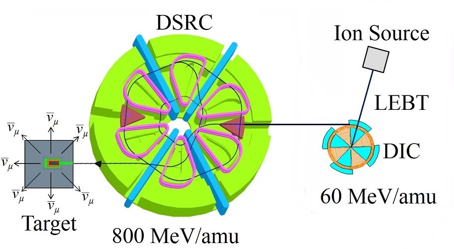
Figure 8: Schematic of the DAE$\delta$ALUS facility. H_2^+ is produced in the ion source, transported to the DAE$\delta$ALUS Injector Cyclotrons (DIC) and accelerated to $60\text{\,}\mathrm{M}\mathrm{e}\mathrm{V}\mathrm{/}\mathrm{a}\mathrm{m}\mathrm{u}$. Ions are subsequently extracted from the cyclotron and injected into the DAE$\delta$ALUS Superconducting Ring Cyclotron (DSRC), where they are accelerated to $800\text{\,}\mathrm{M}\mathrm{e}\mathrm{V}\mathrm{/}\mathrm{a}\mathrm{m}\mathrm{u}$. During the highly efficient stripping extraction, $5\text{\,}\mathrm{e}\mathrm{m}\mathrm{A}$ of H_2^+ becomes $10\text{\,}\mathrm{e}\mathrm{m}\mathrm{A}$ of protons which impinge on the neutrino production target.

At the moment, OPAL-cycl is used for the simulation of three very important parts of the DAE$\delta$ALUS and IsoDAR systems:

1. The spiral inflector

2. The DAE$\delta$ALUS Injector Cyclotron (DIC), which is identical to the IsoDAR cyclotron.

3. The DAE$\delta$ALUS Superconducting Ring Cyclotron (DSRC) for final acceleration.

For the topic of bench-marking, we will restrict ourselves to item 1., the injection through the spiral inflector.

III.2 The Teststand

As mentioned before, the results of the injection tests are reported in detail in Alonso et al. (2015). Here, we will summarize the items pertinent to a comparison to OPAL, specifically, how we obtain the particle distribution at the end of the LEBT (entrance of the cyclotron), used as initial beam in the subsequent injection simulations with the SAAMG solver.

The test stand was comprised of the following parts:

1. Versatile Ion Source (VIS) Miracoli et al. (2012). An off-resonance Electron Cyclotron Resonance (ECR) ion source.

2. The Low Energy Beam Transport (LEBT). The LEBT contained:

   1. First solenoid magnet, for separation of protons and H_2^+.

   2. Beam diagnostics (emittance scanner, faraday cup).

   3. Steering magnets.

   4. Second solenoid magnet (final focusing into the cyclotron).

3. Cyclotron with spiral inflector.

During the experiment, it was possible to transport up to 8 mA of H_2^+ as a DC beam along the LEBT to the cyclotron and transfer 95% of it through the spiral inflector onto a paddle probe. The 4-rms normalized emittances stayed below 1.25 $\pi$-mm-mrad. Capture efficiency into the RF “bucket” was 1-2% because of reduced dee voltage ($\mathrm{V}_{\textrm{dee}}$) due to an under-performing RF amplifier (cf. discussion in Alonso et al. (2015)).

III.3 Initial Conditions

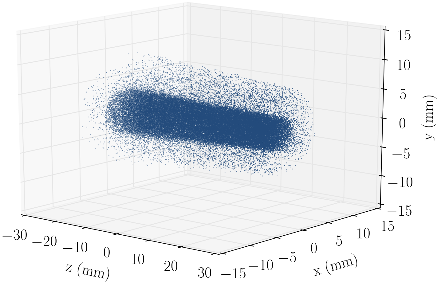
Figure 9: Initial distribution for injection through the spiral inflector, obtained by carefully simulating the LEBT Alonso et al. (2015). The length of the bunch corresponds to one full RF period at $49.2\text{\,}\mathrm{M}\mathrm{H}\mathrm{z}$ and injection energy of $62.7\text{\,}\mathrm{k}\mathrm{e}\mathrm{V}$, centered at the synchronous phase, thus, to first order, representing a DC beam.

The quality of any simulation result depends on the initial conditions. In the case of the OPAL SAAMG simulations of the injection through the spiral inflector, the initial particle distribution consisted of 66021 particles obtained by carefully simulating the ion source extraction (using KOBRA-INP Spädtke (2000)) and the subsequent LEBT (using WARP Grote et al. (2004)) and comparing the simulation results to the measurements, with good agreement as reported in Alonso et al. (2015). During the WARP simulations of the LEBT, the “xy-slice-mode” was used in which the self-fields are calculated only for the transverse direction (assuming only very slow changes in beam diameter along the z-axis compared to the length of each simulation step) and neglecting longitudinal self-fields (which is a sensible approach for DC beams). Space charge compensation played a big role in order to obtain good agreement and was taken into account using a semi-analytical formula Winklehner and Leitner (2015). The final particle distribution that was obtained for the set of parameters recorded during the measurements is shown in Figure 9. It should be noted that the bunch was generated from the xy-slice at a position 13 cm away from the cyclotron mid-plane and coaxial with the cyclotron center by randomly backward and forward-projecting particles according to their respective momenta. It can be seen that this beam enters the spiral inflector converging, which has been found experimentally to give the best injection efficiency. The important parameters of the injected beam are listed in Table 1.

Table 1: Beam and cyclotron parameters for inflection and acceleration studies.

Parameter	Value
Species	H_2^+
Initial Beam Energy	62.7 keV
2-rms Beam Diameter	10.6 mm
4-rms Normalized Emittance	1.19 $\pi$-mm-mrad
Cyclotron Magnetic Field	1.1 T average
Spiral Inflector Upper / Lower	-10.0 kV/+10.15 kV
Beam Current	7.0 mA
Approximate Dee Voltage	$\approx 60$ kV

III.4 Results

The beam described in the previous section was then transported through the spiral inflector using the standard FFT and the new SAAMG field solver described in Section II.3, and putting in place the geometry seen in Figure 3.

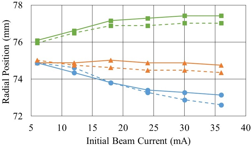
Figure 10: Radial positions of the peak of each finger of the five-finger probe (cf. text). Blue (circles): Finger 2, orange (triangles): Finger 3, green (squares): Finger 4, solid: FFT, dashed: SAAMG.

Inside the cyclotron, 45^∘ after the exit of the spiral inflector, a radial probe was placed which had 5 fingers of $\approx 5$ mm vertical extent, and $\approx 1$ mm radial extent each. On these fingers, the electrical beam current was measured. The probe was slowly moved from a position blocking the beam completely, to just outside of the radial extent of first turn, thereby giving the beam current distribution shown in the top plot of Figure 11. In the same plot, the results from OPAL simulations using the same parameters as recorded during the measurement (see Table 1) are plotted. Good qualitative agreement can be seen for both the FFT and the SAAMG solver. Due to the tail towards low radius, two Gaussians are used to fit each peak in the left column. The full widths at half maximum (FWHM) of the dominant Gaussians are listed in Table 2. There seems to be a slight shift towards higher vertical position that is better reproduced in the SAAMG solver, but this is well within the systematic errors of the measurement and how well the initial parameters like magnetic field, spiral inflector voltage and beam distribution were known, hence the conclusion is that both FFT and SAAMG reproduce the measured radial–vertical beam distribution equally well for a 6 mA beam. This shows that the SAAMG solver is working as expected.

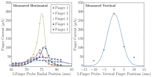
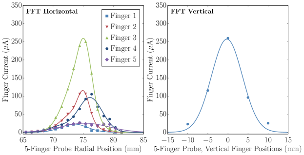
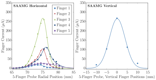
Figure 11: Measurement and simulation of a 5-finger probe (for description cf. to text) in the first turn of the BCS test cyclotron central region, 45^∘ after the exit of the spiral inflector. Each finger has a main peak and a tail towards lower radius. These are the particles that are not sufficiently accelerated. To guide the eye and to compare with the simulations, the data for each finger is fitted with two Gaussians.

Table 2: Full width at half maximum (FWHM) for the measured distribution and the OPAL results using the FFT and the SAAMG solver.

	Measured	FFT	SAAMG
Finger 1	16.26 mm	5.21 mm	5.47 mm
Finger 2	1.64 mm	2.19 mm	2.19 mm
Finger 3	2.03 mm	2.61 mm	2.52 mm
Finger 4	2.15 mm	4.75 mm	2.50 mm
Finger 5	12.31 mm	9.26 mm	9.28 mm
Vertical	8.22 mm	9.05 mm	8.99 mm

III.4.1 Higher beam currents

For initial beam currents up to 36 mA, the results of the FFT and SAAMG solvers start to show stronger (but still fairly subtle) discrepancies which can be attributed to the image charges on the electrodes only included with the SAAMG solver. An example is shown in Figure 10 where the expected spreading of the peak positions is accompanied by a noticeable overall shift towards smaller radii in case of the SAAMG solver.

IV Conclusion

IV.1 Summary and Discussion

For the first time a comprehensive and precise beam dynamics simulation model, from the ion source, throughout the LEBT, into the central region of a cyclotron was presented. The central region includes the spiral inflector and the first accelerating gap. From the exit of the LEBT, the open source code OPAL was used for the beam transport through the spiral inflector and the first turn of the test cyclotron. Key ingredients of the model are the the flexible handling of the complex geometry, and the field solvers for space charge calculation. In comparison with first measurements, both the FFT and the SAAMG solver perform well, with hints that image charge effects become more important at higher currents, where use of the SAAMG solver allows including the complicated boundary conditions posed by the electrode system. These ingredients - geometry and field solvers (FFT and SAAMG) are now included with OPAL. Validation of the model included simple test cases and comparison to measurements from a dedicated cyclotron test stand, injecting a DC beam of 7 mA of H_2^+. Both yielded good agreement. The level of detail available in this model now allows us to obtain a detailed understanding, and predict the complicated beam dynamics in the high current compact IsoDAR cyclotron.

IV.2 Outlook

Given this benchmarked model, a full start to end simulation of the IsoDAR cyclotron is ongoing, using first the detailed geometry for acceleration up to 1 MeV/amu, and then a simplified model with FFT only for the subsequent acceleration up to $60\text{\,}\mathrm{M}\mathrm{e}\mathrm{V}\mathrm{/}\mathrm{a}\mathrm{m}\mathrm{u}$. Recently, a proposal was put forward to test direct injection into the compact IsoDAR cyclotron using a Radio Frequency Quadrupole (RFQ) Winklehner et al. (2016). For the design of this device, OPAL-cycl and the new SPIRAL mode will play an essential role.