Synthesis of Tongue Motion and Acoustics From
Text using a Multimodal Articulatory Database

Abstract

We present an end-to-end text-to-speech (TTS) synthesis system that generates audio and synchronized tongue motion directly from text. This is achieved by adapting a 3D model of the tongue surface to an articulatory dataset and training a statistical parametric speech synthesis system directly on the tongue model parameters. We evaluate the model at every step by comparing the spatial coordinates of predicted articulatory movements against the reference data. The results indicate a global mean Euclidean distance of less than 2.8 mm, and our approach can be adapted to add an articulatory modality to conventional TTS applications without the need for extra data.

I Introduction

The sound of human speech is the direct result of production mechanisms in the human vocal tract. Air flows from the lungs through the glottis, whose vocal folds can be set to vibrate, the sound of which is then filtered by the shape of the tongue, lips, and other articulators, generating what we perceive as audible signals such as spoken language. Researchers in phonetics and linguistics have studied these speech production mechanisms for many years, but while the acoustic signal and facial movements can be observed and measured directly, doing the same for partially or fully hidden articulators such as the tongue and glottis is not as straightforward.

Consequently, sensing and imaging techniques have been applied to the challenge of observing speech production mechanisms in vivo, which has greatly improved our understanding of these processes. The corresponding modalities include, fluoroscopy [1], UTI [2], XRMB [3], EMA [4, 5], and real-time MRI [6, 7], among others. Some of these involve health hazards (due to ionizing radiation), and all are more or less invasive, but they produce biosignals which, in combination with simultaneous acoustic recordings, represent multimodal articulatory speech data. The benefits are tempered by the challenges of processing the imaging and/or point-tracking data, which in the field of speech processing has created new opportunities for collaboration with areas such as medical imaging and computer vision.

The biosignals that can be obtained using such modalities to record spoken language, provide opportunities to greatly enhance models of speech by integrating measurements of the underlying processes directly with the acoustic signal. This leads to more elegant and powerful approaches to speech analysis and synthesis [8, 9, 10]. However, it must be borne in mind that all of the biosignals produced by the modalities mentioned above represent a sampling of the articulators that is sparse in the temporal domain, the spatial domain, or both.

Depending on the manner in which the data is used for analysis or applications, the resolution may need to be increased, but the missing samples cannot be restored without prior knowledge, typically provided by a statistical model trained on other data.

In this study, we present an approach to multimodal TTS synthesis that generates the fully animated, 3D surface of the tongue, synchronized with synthetic audio, using data from a single-speaker, articulatory corpus that includes EMA motion capture of three tongue fleshpoints [11]. The audio and articulatory motion are synthesized using the HTS framework [12], while the surface restoration is performed by means of a multilinear statistical tongue model [13] trained on a multi-speaker, volumetric MRI dataset [14]. The potential application domains of this approach include audiovisual speech synthesis and CAPT, among others.

I-A Background

Deriving models suitable for producing speech related tongue motion is an active field of research. Such models can, for example, help to analyze and understand articulatory data that is very sparse in the spatial domain. Ideally, such tongue models should offer a good compromise between accuracy of the generated shape and the available DoF for manipulating it. This means that biomechanical models such as those presented by [15], [16], [17], or [18] might be too complex for this purpose. While such models aim to simulate the underlying mechanics of the human tongue as closely as possible, and can be used to visualize existing articulatory data, they can be challenging to control efficiently.

Geometric tongue models are less complex than their biomechanical counterparts. Here, we distinguish between generic and statistical tongue models. Generic tongue models are 3D models of the tongue that may be deformed and animated by using standard methods in computer graphics.

Statistical tongue models, on the other hand, are constructed by analyzing the DoF of the tongue shape in recorded articulatory data, such as MRI recordings of speech related vocal tract shapes. Roughly speaking, such an analysis can be carried out in two ways. The first variant investigates shape variations related to the tongue pose that are specific for speech production. Examples of such approaches are the works by [19, 20], and [21], who examined those variations in 3D MRI scans from a single speaker, respectively. These methods only estimate the DoF that are tongue pose related, while shape variations that may describe anatomical differences are missing.

Another class of methods aims at investigating those anatomy and tongue pose related shape variations separately. This paradigm offers several advantages: First, the results give access to tongue models that may be adapted to new speakers. Second, this type of analysis may also provide insight into how anatomical differences affect human articulation. For 2D MRI, such work was conducted, e.g., by [22] and [23]. [24] investigated those variations in a sparse point cloud extracted from 3D MRI. Most recently, we performed such an analysis on mesh representations of the tongue that were extracted from 3D MRI scans [13].

Such geometrical models have been successfully used in previous work to generate animations from provided articulatory data: [25] presented a real-time visual feedback system that deforms a generic tongue model using EMA data. However, due to the generic nature of the model, their approach did not take anatomical differences into account. A statistical model was used in the approach by [26], who used volumetric imaging data of one speaker to derive the tongue model, and EMA data of the same speaker to animate it. [27] followed a similar approach. Our own previous work utilized a multilinear statistical model to visualize EMA data, which allowed it to be adapted to different speakers [28].

Independently, there is a growing body of work on application-oriented research to combine articulatory data, and features derived from it, with speech technology applications, such as to recover articulatory movements from the acoustic signal (“articulatory inversion mapping”, cf. [29, 30] for examples), provide articulatory control for reactive TTS synthesis (e.g., [31, 32]), or predict sparse articulatory movements from a symbolic representation (e.g., [9, 33]).

Early studies on animating full 3D tongue surface models using EMA data for multimodal speech synthesis, such as those of [34] or [35], used concatenative TTS systems. Other approaches (e.g., [36]) for HMM based TTS with intra-oral animation also rely on acoustic-articulatory inversion mapping. However, to our knowledge, no previous study has presented an end-to-end system to directly synthesize acoustics and the motion of a full 3D model of the tongue surface from text using statistical parametric speech synthesis, particularly with a tongue model that can be easily adapted to the anatomy of different speakers.

II Method

II-A Multilinear Shape Space Model

In our approach, we utilize a multilinear model to describe different tongue shapes. This is achieved by using this model to create a function

$$f:\mathbb{R}^{m}\times\mathbb{R}^{n}\to\mathcal{M}$$ (1)

that maps the parameters $\vec{s}\in\mathbb{R}^{m}$ and $\vec{p}\in\mathbb{R}^{n}$ to a polygon mesh $M=(V,F)\in\mathcal{M}$. Such a mesh consists of a vertex set $V:=\{\vec{v}_{i}\}$ that contains positional data $\vec{v}_{i}\in\mathbb{R}^{3}$ and a face set $F$ that uses these vertices to form the collection of surface patches of the represented shape. We note that these meshes $M$ have the same face set and only differ in the positional data of their vertices. The used parameters in the function describe two distinct sets of features: On the one hand, the speaker parameter $\vec{s}$ determines the anatomical features of the generated tongue. The pose parameter $\vec{p}$, on the other hand, represents the shape properties that are related to articulation.

To compute the multilinear model, we use a database that consists of MRI scans of $m$ speakers showing their vocal tract configuration for $n$ different phonemes. By means of image processing and template matching methods, we extract tongue meshes $M\in\mathcal{M}$ from the MRI data, such that in the end, for each speaker, one mesh is available for each considered phoneme. This processing is described in detail by [37, 13]. We then proceed to derive the DoF of the anatomy and speech related variations. To this end, we center the obtained meshes and turn them into feature vectors by serializing the positional data of their vertices. Afterwards, we construct a tensor $A$ of third order consisting of these feature vectors, such that the first mode of the tensor corresponds to the speakers, the second one to the considered phonemes, and the third one to the positional data.

In a final step, we apply HOSVD [38] to obtain the following tensor decomposition:

$$A=C\times_{1}U_{1}\times_{2}U_{2}$$ (2)

In this decomposition, the tensor $C$ is of third order and represents our multilinear model. The operation $C\times_{n}U$ is the $n$-th mode multiplication of the tensor $C$ with the matrix $U$. The two matrices $U_{1}\in\mathbb{R}^{m\times m}$ and $U_{2}\in\mathbb{R}^{n\times n}$ contain the parameters for reconstructing the original feature vectors: Each row of $U_{1}$ is a speaker parameter and each row of $U_{2}$ a pose parameter. Basically, each speaker parameter represents a point in the $m$-dimensional speaker subspace and each pose parameter a point in the $n$-dimensional pose subspace that are linked together by the tensor $C$. We remark that, compared to a PCA model, such a multilinear model offers the advantage that it aims at capturing anatomical and articulation related shape variations separately.

The tensor $C$ can be used to create new positional data for provided parameters $\vec{s}$ and $\vec{p}$:

$$v(\vec{s},\vec{p})=\mu+C\times_{1}\vec{s}\times_{2}\vec{p}$$ (3)

where $\mu$ is a feature vector consisting of the positional data that corresponds to the mean mesh of the tongue shape collection. This generated information can be utilized to construct a new tongue shape: We reconstruct the vertex set by using the created positional data and combine it with the original face set to obtain our mesh. More details on how the model was derived and evaluated can be found in [13].

Figure 1: Rendered tongue model mesh, highlighting three vertices selected to correspond to the tongue coils in the EMA data; pink: T1, yellow: T2, purple: T3 (cf. Fig. 3).

In our framework, we use this model to register data of an EMA corpus in order to obtain the corresponding parameters, which is done as follows: In a first step, we manually align the EMA data to the model space by using a provided reference coil. As we want to register the EMA data, we have to decide which coil corresponds to which vertex of the model mesh. This process is done in a semi-supervised way: The parameters are first set to random values and the associated mesh $f(\vec{s},\vec{p})$ is generated. Next, for each considered coil the nearest vertex on the mesh is found. We then refine these correspondences iteratively by fitting the model to the coils and updating the nearest vertices. In the end, we keep the correspondences that resulted in the smallest average Euclidean distance. Finally, we inspect the result manually and repeat the experiment if the correspondences appear to be wrong. The tongue model mesh is shown in Fig. 1, highlighting the vertices selected to correspond with the three tongue coils in the EMA data. With these estimated correspondences, we fit the multilinear model to each considered EMA data frame of the corpus by minimizing the energy:

$$E(\vec{s},\vec{p})=E_{\text{Data}}(\vec{s},\vec{p})+\alpha\ E_{\text{SC}}(\vec{s})+\beta\ E_{\text{PS}}(\vec{p})$$ (4)

The data term $E_{\text{Data}}(\cdot)$ measures the distances between the selected vertices of the generated mesh $f(\vec{s},\vec{p})$ and the corresponding coil positions. The speaker consistency term $E_{\text{SC}}(\cdot)$ weighted by $\alpha>0$ generates energy if the current speaker parameter differs from the one of the previous time step. The remaining term, the pose smoothness term $E_{\text{PS}}(\cdot)$ weighted by $\beta>0$ fulfills a similar role: It penalizes changes of the pose parameter over time. As a minimizer of this energy is the best compromise between those mentioned assumptions, the fitting results will be close to the data and show smooth transitions over time. The degree of smoothness can be controlled by adjusting the weights $\alpha$ and $\beta$. As the multilinear model can be used to measure the probability of generated shapes, we can also choose how far the results are allowed to deviate from the model mean: We limit the possible values for each entry of the parameters to an interval $[m_{i}-c\ \sigma_{i},m_{i}+c\ \sigma_{i}]$ where $c>0$, $m_{i}$ is the mean and $\sigma_{i}$ the standard deviation of the corresponding entry in the training set of tongue meshes. In order to obtain a minimizer, we use a quasi-Newton solver [39] that supports limiting the solution to the given intervals.

II-B Multimodal Statistical Parametric Speech Synthesis

HTS

The HTS framework first presented by [40] is a standard statistical parametric speech synthesis system. The architecture comprises four main parts:

1. the parametrization of the signal,

2. the training of the models,

3. the parameter generation, and

4. the signal rendering.

The focus of our study impacts the parametrization (a) and the rendering (d) stages. Therefore, we use the standard training stage (b), described in [40], and the standard parameter generation algorithms (c), described in [41].

The parametrization of the signal can be performed using any suitable signal processing tool, as long as it is kept consistent with the signal rendering. In the standard procedure, this is generally accomplished by coupling STRAIGHT [42] with a MLSA filter [43]. First, STRAIGHT is used to extract the spectral envelope, the F0, and the aperiodicity. Generally, the F0 values are transformed into the logarithmic domain, to be more consistent with human hearing. Since the number of coefficients used of the spectral envelope and the aperiodicity is too high, the MLSA filter is used to parametrize these coefficients and to obtain the MGC and the BAP, respectively.

In this study, we propose to not only consider the parametrization of the acoustic signal but also the parametrization of speech articulation. In previous studies [8, 44, 9], EMA data was used as the articulatory representation. In the present study, we work towards replacing the EMA data by the tongue model parameters. Therefore, our goal is to train on the trajectories of the tongue model parameters using the standard HTS framework as presented by [40]. The training models in HTS are HMM, at a phone level, whose observations are composed by decision trees. The leaves of the decisions trees are GMM which are used to produce the parameters at the generation level. The generation level consists of applying the algorithm presented by [41]. Fig. 2 presents the details of the modified architecture.

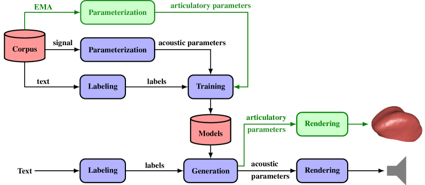
Figure 2: Architecture for multimodal HMM based synthesis adapted from [40]; the multimodal extensions are highlighted.

III Experiments

III-A Multilinear Model

As the database for deriving the multilinear model, we used MRI data from the Ultrax project [14] (11 speakers) and combined it with the data of [45] (1 speaker), which was recorded as part of the Ultrax project, but released separately. In the end, the resulting tongue mesh collection contained, for each speaker, estimated shapes for the phone set [i, e, E, a, A, 2, O, o, u, 0, @, s, S]. Accordingly, the resulting multilinear model has $12\text{\,}\ac{DoF}13\text{\,}\ac{DoF}$ for the anatomy and tongue pose, respectively. The tongue mesh we used for the template matching was manually extracted from one MRI scan, made symmetric to remove some bias towards the original speaker, and finally remeshed to be more isotropic. It consists of $3100$ vertices, $6102$ faces, and has a spatial resolution of $1.87\text{\,}\mathrm{mm}$.

III-B Database

The data used for the experiments in this study is taken from the mngu0 corpus, specifically the “day 1” EMA subset [11], which contains acoustic recordings, time-aligned phonetic transcriptions, and EMA motion capture data (sampled at $200\text{\,}\mathrm{Hz}$ using a Carstens AG500 articulograph). We selected the “basic” (as opposed to the “normalized”) release variant of the EMA data, because it preserves the silent (i.e., non-speech) intervals, as well as the 3D nature and true spatial coordinates of the sensor data (after head motion compensation). The EMA coil layout for this data is shown in Fig. 3; the coils are explained in Table I.

In order to manipulate the EMA data more flexibly, the files were first converted from the binary EST format to a JSON structure. Invalid values (i.e., NaN) were replaced by linear interpolation. No further modification, in particular no smoothing, was applied.

From the provided acoustic data, signal parameters were extracted using STRAIGHT [42] with a frame rate of $200\text{\,}\mathrm{Hz}$, matching that of the EMA data. As we follow the standard HTS methodology, we also kept the same parameters. Therefore, our signal parameters are $50\text{\,}\ac{MGC}$, $25\text{\,}\ac{BAP}$, and one coefficient for the F0.

From the $1354$ utterances in the data, $152$ ($11.2\text{\,}\mathrm{\char 37\relax}$, around $10\text{\,}\mathrm{min}$) were randomly selected and held back as a test set; the remaining $1202$ utterances (around $105\text{\,}\mathrm{min}$) were used as the training set to build HTS synthesis voices. A comparison of phone distributions in the training and test sets shows a satisfactory match (cf. Fig. 4).

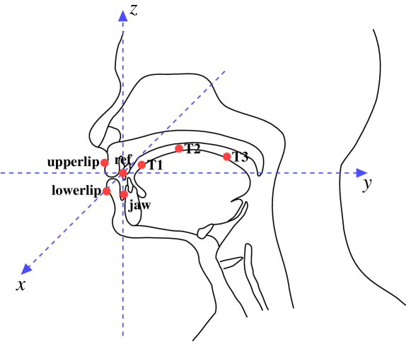
Figure 3: EMA coil layout in the “day 1” subset of the mngu0 corpus. All coils are close to the mid-sagittal plane. The ref coil on the upper incisors forms the origin of the coordinate space; the horizontal and vertical axes represent the $y$ and $z$ dimensions in the data, respectively, while the $x$ axis is perpendicular to the image plane. Adapted from [11].

Table I: EMA Coil Labels and Locations in the “Day 1” Subset
of the mngu0 Corpus.

Label	Location
T1	Tongue tip
T2	Tongue body
T3	Tongue dorsum
upperlip	Upper lip
lowerlip	Lower lip
ref	Upper incisor
jaw	Lower incisor

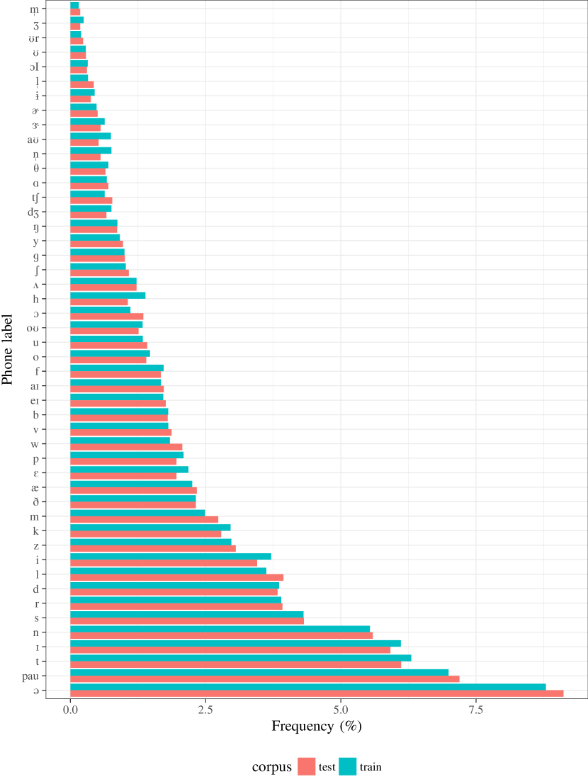
Figure 4: Distribution of phones across the training and test sets.

III-C Acoustic Synthesis

Table II: Global Evaluation Measures for the Acoustic Synthesis Baseline Conditions.

As a baseline, we first built a conventional TTS system using the acoustic data only. This served mainly to validate our voicebuilding process and ensure that the transcriptions provided, and labels generated from them, along with the acoustic signal parameters, were able to generate audio of sufficient quality. Accordingly, we did not undertake a formal subjective listening test, and instead evaluated this baseline experiment using objective measures only.

We synthesized the $152$ utterances in the test set using two conditions. The first condition is the standard synthesis process. This condition allows us to evaluate the duration accuracy. For the second condition, we imposed the acoustic phone durations from the provided transcriptions to allow direct comparison with the natural recordings. For the following experiments, we synthesized both conditions as well. The objective evaluation was conducted based on the following metrics.

For the duration evaluation, we calculated the duration RMSE at the phone level (in $\mathrm{ms}$) between the reference duration and the one synthesized using the first condition.

Considering the other coefficients, we compared the synthesis result ($s$), achieved using the second condition, to the reference ($r$) present in the test corpus. As the duration was imposed, we have the same number $T$ of frames for the produced utterance and the reference one. To evaluate the F0, we used three measures: the VUV error rate percentage $VUV(r,s)$ 6 to check the prediction of the F0, the RMSE in $\mathrm{Hz}$ 7, and the RMSE in cent 8. The latter measure focuses on the frames which are voiced in both conditions (original and predicted F0). Furthermore, it is a log scale measure adapted to the human perception.

$$v(x,y)=\left\{\begin{array}[]{ll}0&\text{x \& y are both voiced/unvoiced}\\ 1&\text{otherwise}\\ \end{array}\right.$$ (5)

$$VUV(r,s)=(\sum_{t=1}^{T}v(r_{t},s_{t})/T)*100$$ (6)

$$RMSE_{$\mathrm{Hz}$}(r,s)=\sqrt{\sum_{t=1}^{T}(r_{t}-s_{t})^{2}/T}$$ (7)

$$RMSE_{\text{cent}}(r,s)=\sqrt{1200*\sum_{t=1}^{T}(log(r_{t})-log(s_{t}))^{2}/T}$$ (8)

Finally, to evaluate the spectral envelope production, we computed the MCD between the MGC vectors of dimension $M$ in $\mathrm{dB}$:

$$d(x,y)=\sum_{m=2}^{M}(x(m)-y(m))^{2}$$ (9)

$$MCD(r,s)=\frac{10}{\ln 10}*\sqrt{2}*\sqrt{\sum_{t=1}^{T}d(r_{t},s_{t})/T}$$ (10)

Except for the duration, all parameters were evaluated at the frame level. Based on these measures, we can compare our results to previous studies, such as the one presented by [46].

The results of this evaluation are given in Table II and comprise the mean, standard deviation, and confidence interval with a $p$ value at $5\text{\,}\mathrm{\char 37\relax}$. Compared to [46], we achieved slightly better results, notwithstanding the different dataset. Therefore, we can conclude that our acoustic prediction is consistent with the state of the art in HTS.

III-D Combined Acoustic and EMA Synthesis

Adopting the paradigm of early multimodal fusion, we combined the acoustic signal parameters with the 3D positions of the seven EMA coils shown in Table I, increasing the vector size by $21$, to $97$ parameters per frame. Using the HTS framework, we then built another TTS system from this multimodal data.

Synthesizing the test set in this way, we obtained, in addition to the audio, synthetic trajectories of predicted EMA coil positions. To evaluate the combined acoustic and EMA synthesis, we computed the same objective measures as in Section III-C. We also computed the Euclidean distance in space between the observed and predicted positions for the EMA coils. Finally we computed the RMSE between the dynamics of the trajectories of the coils using a unit of millimeters per frame ($\mathrm{m}\mathrm{m}\mathrm{/}\mathrm{f}\mathrm{r}\mathrm{a}\mathrm{m}\mathrm{e}$). The results of this evaluation are given in Table III. We see that the differences in the acoustic measures compared to the acoustic-only synthesis (cf. Table II) are negligible.

The comparison between the observed and predicted trajectories for one test utterance is illustrated in Fig. 5. The observed and predicted (synthesized) positions of the three tongue coils are shown in each of the three dimensions in the data, along with the Euclidean distance. Silent intervals and consonants classified as coronal [t, d, n, l, s, z, S, Z, T, D] and dorsal [g, k, N], based on the provided phonetic transcription, have been highlighted. This helps visualize the correspondence between gestures of the tongue tip (coil T1) and tongue back (coils T2 and T3) for coronal and dorsal consonants, respectively, and the phonetic units they produce.

Several points merit discussion. First of all, there are large mismatches between the observed and predicted tongue EMA coil positions during the silent (pause) intervals at the beginning and end of the utterance. This can be attributed to the fact that the wide range of the speaker's tongue movements during non-speech intervals are not distinguished in the provided annotations, but invariably labeled with the same pause symbol. However, there are at least two very distinct shapes for the tongue during such silent intervals, including a “rest” and a “ready” position (just before speech is produced), in addition to other complex movements such as swallowing. In the absence of distinct labels corresponding to these positions and movements, none of this silent variation can be captured by the HMM trained on this data; instead, the tongue coils are unsurprisingly predicted to hover around global means.

Secondly, there is noticeable oversmoothing and target extrema are not always quite reached. This can typically be attributed to the HMM based synthesis technique, despite the integration of global variance. The dynamics, however, are well represented, and the predicted positional trajectories, as well as their derivatives, match the observed reference quite closely.

The $x$ axis appears to suffer from a greater amount of prediction error than the $y$ or $z$ axes. However, it should be noted that the positional variation along the $x$ axis is an order of magnitude smaller than that along the $y$ axis. It must also be borne in mind that nearly all of the speech-related movements occur in the mid-sagittal plane, represented by the $y$ (anterior/posterior) and $z$ (inferior/superior) axes; variation along the $x$ axis corresponds to lateral movements, which are infrequent during speech. Having said that, the $x$ axis can serve to illustrate the physical coil locations on the tongue in the “day 1” recording session; to wit, the tongue tip coil is actually attached out of plane, a few millimeters to one side.

The Euclidean distances during speech are in the millimeter range, indicating that the predictions of EMA coil positions are accurate to within the precision of the EMA measurements themselves. However, there appears to be a certain amount of fluctuation with a more or less regular range and shape. The peaks of this fluctuation appear to correlate with spikes in the rms channels of the provided EMA data, which supports the hypotheses that it is either an artifact of the algorithm which calculates the coil positions and orientations from the raw amplitudes [47], or measurement noise in the articulograph itself [48], or, conceivably, a combination of both factors. Of course, the noise in the Euclidean distance analysis is a direct consequence of our decision to refrain from smoothing the provided EMA data.

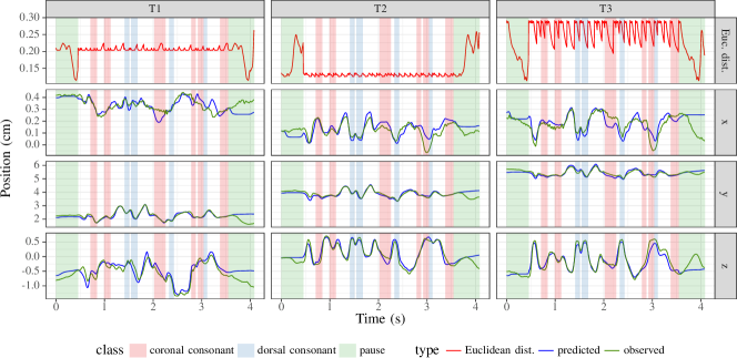
Figure 5: Observed and predicted position trajectories (along the $x$, $y$, and $z$ axis), and Euclidean distance (top), for the tongue EMA coils (T1, T2, T3) for one test utterance, using combined acoustic and EMA synthesis. The utterance is “Because these deer are gregarious, they go about in groups”. Based on the provided transcriptions, intervals containing silent (pause) and coronal and dorsal consonants have been highlighted.

Table III: Global Evaluation for the Combined Acoustic and EMA Synthesis.

III-E EMA Synthesis

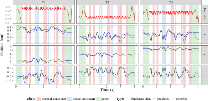
Figure 6: One test utterance produced using EMA-only synthesis; all other details are the same as in Fig. 5.

Table IV: Global Evaluation for the EMA-Only Synthesis.

While the combined acoustic and EMA synthesis produced satisfactory results, the requirement to train the system on a multimodal dataset such as mngu0 represents a significant drawback; compared to the reasonably wide availability of conventional, acoustic databases designed for speech synthesis, the number of suitable articulatory databases is extremely low. Encouraged by the practical equivalence in the evaluation of the acoustic measures described in Sections III-C and III-D, we therefore considered the question of decoupling the EMA synthesis completely from the acoustic data. Accordingly, we used the HTS framework to build another TTS system trained only on the EMA data, without the acoustic parameters.

Under this condition, the evaluation of the duration RMSE and Euclidean distances between the predicted and observed EMA coils, computed using the formula given by 7, is given in Table IV. As we can see, the results are nearly identical to those in Table III, which confirms the validity of this approach. Fig. 6 visualizes the comparison between the observed and predicted trajectories for one test utterance.

III-F Tongue-only EMA Synthesis

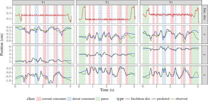
Figure 7: One test utterance produced using EMA-only synthesis restricted to the tongue coils; all other details are the same as in Fig. 5.

Table V: Global Evaluation for the EMA-Only Synthesis Restricted to the Tongue Coils.

In order to focus on the tongue in the following section, we first needed to investigate how far the tongue coil EMA positions can be predicted in isolation from the remaining EMA coils. To this end, we created a modified version of the TTS system described in the previous section, by including only the tongue coils (T1, T2, and T3), and excluding the rest of the EMA data from the training set.

Table V gives the evaluation of the EMA synthesis restricted to the three tongue coils. Comparing these results with those in Table IV, we observe that the values are virtually identical, which confirms the validity of this approach. As before, the comparison between the observed and predicted trajectories for one test utterance is shown in Fig. 7. It should be noted that despite the removal of the EMA coil on the lower incisor, some residual jaw motion is implicitly retained in the movements of the tongue coils.

III-G Model-based Tongue Motion Synthesis

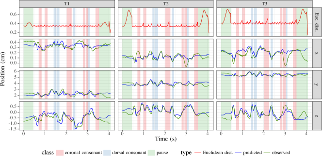
Figure 8: One test utterance produced using the tongue model parameters synthesis; all other details are the same as in Fig. 5.

Table VI: Global Evaluation for the Tongue Model Parameters Synthesis.

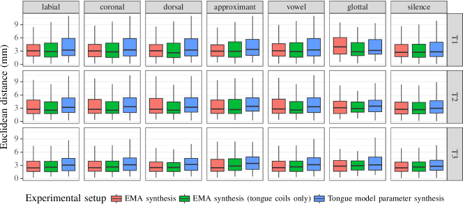
Figure 9: Distributions of Euclidean distances between observed and predicted tongue EMA coil positions for each experimental TTS setup, split by phone class and tongue EMA coil.

At last, having verified that the HTS framework can be used to synthesize audio and predict the movements of three tongue EMA coils using separate models trained on the mngu0 database, we prepared a new kind of TTS system to predict the shape and motion of the entire tongue surface, by integrating the multilinear model into the process.

To this end, we first estimated the anatomical features $\vec{s}$ (cf. Section II-A) of the speaker in the mngu0 dataset as follows: We used the upper incisor coil as a reference and estimated the correspondences between the three tongue coils and the model vertices, chosen as described in Section II-A. During this correspondence optimization, we used $c=0.25$. Thus, we limit the admissible values for each entry of the model parameters to the interval $[m_{i}-0.25\ \sigma_{i},m_{i}+0.25\ \sigma_{i}]$ where $m_{i}$ is the mean and $\sigma_{i}$ the standard deviation of the corresponding model parameter. By using such a small interval, we try to prevent overfitting during this step. Afterwards, we fitted the model to all EMA data frames and stored the obtained parameter values. Here, we used the speaker consistency weight $\alpha=20$ and the pose smoothness weight $\beta=10$ in the fitting energy. Thus, we demanded very smooth transitions in this case and especially penalized changes of the speaker's anatomy over time. In this step, we used $c=3$ to give the approach some freedom during the fitting. We then averaged all obtained speaker parameters to get an estimate of the considered speaker's anatomical features.

Next, we again fitted the model to all EMA data frames where, this time, we fixed the speaker parameter $\vec{s}$ to the estimated anatomy. We note that this approach causes the multilinear model to behave like a single-speaker PCA model. This time, we used the weight $\beta=1$ to increase the influence of the data term. However, we decided to use $c=2$ this time to motivate the approach to consider more plausible shapes.

We note that the settings for the fitting were selected manually by an expert. Of course, this selection might be optimized for the used EMA dataset by performing a thorough analysis.

The pose parameters resulting from this fitting step were taken as the training data, and we used the HTS framework to build a new TTS system that predicts the tongue model parameter values directly from the input text.

To evaluate the performance of this system against the reference EMA data, we extracted the spatial coordinates of the vertices assigned during the adaptation step (see above) to produce synthetic trajectories that served as a virtual surrogate for predicted EMA data.

We evaluated this synthetic EMA data against the reference as before; Table VI provides the Euclidean distances between the predicted and observed EMA coils, and one test utterance is visualized in Fig. 8. It should be noted that the tongue model itself contains a temporal smoothing term, which ensures that a noisy sequence of input frames does not cause the 3D mesh to change shape or position too rapidly; however, this extra smoothing contributes to widespread target undershoot in the comparison. Overall, the results of this evaluation are very promising, and we can confirm that as far as possible, with only three surface points on the tongue, the animation of the full tongue appears to closely match the observed reference.

Finally, in order to compare the three experimental TTS systems (trained without acoustic data), we analyzed the distribution of Euclidean distances between each system and the observed reference data over the entire test set; the results are shown in Fig. 9. The distances are slightly greater when the non-tongue EMA coils are excluded, and greater still when the EMA prediction is replaced by the direct synthesis of tongue model parameters. However, overall, the distances remain in the same range, which indicates that the latter approach perform no worse than synthesis of EMA data – while adding the full 3D tongue surface into the synthesis process.

IV Conclusion

In this study, we have presented a new process of synthesizing acoustic speech and synchronized animation of a full 3D surface model of the tongue. We used the HTS framework with a single-speaker, multimodal articulatory database containing EMA motion capture data. First, we demonstrated a conventional, fused multimodal approach, then separated the two modalities while ensuring that the objective evaluation measures remained comparable. Finally, we adapted a multi-linear statistical model of the tongue and integrated it into the TTS process, and evaluated its accuracy by comparing the spatial coordinates of vertices on the model surface to the reference EMA data from the original speaker's tongue movements. The results are very encouraging, and we believe that this will enable multimodal TTS applications that provide tongue animation with human-like performance.

It should be noted that the acoustic synthesis and predicted phone durations need not come from the same corpus as the one used for training the tongue model parameter synthesis system. Under certain conditions, it would be straightforward to use a different, conventional TTS system with speech recordings from a different speaker in combination with this tongue model parameter synthesis, perhaps adapting it in the speaker subspace automatically or by hand, to generate a multimodal TTS application with plausible, speech-synchronized tongue motion, without the requirement of having articulatory data available for the target speaker. In this way, it is possible to first synthesize the acoustic speech signal, and to provide the predicted acoustic durations to guide the synthesis of corresponding tongue model parameters, which are then used to render the animation of the 3D tongue model in real time.

However, there is clearly more work to be done, and in future research, we intend to refine and improve our system, and to evaluate it using human subjects who will rate it perceptually. Such a study can include intelligibility, such as the contribution of visible tongue movements during degraded, noisy, or absent audible speech. However, we also plan to assess the impact on perceived naturalness by integrating the tongue model into a realistic talking avatar (e.g., [49, 50]), and investigating the importance of naturalistic tongue movements for the overall impression of such avatars in multimodal spoken interaction scenarios with artificial characters. This may also lead us to model distinct non-speech poses for the tongue, such as separate “rest” and “ready” positions.

Regarding the tongue model integration, we plan to further investigate such factors as the impact of reducing the dimensionality of the model subspaces on synthesis performance, optimizing the vertex correspondence with EMA data, improving the fitting results by adjusting the weights for the smoothness terms, and exploring speaker adaptation using volumetric data, such as the MRI subset of the mngu0 corpus [51].

References

- [1] Kevin G. Munhall, Eric Vatikiotis-Bateson and Yoh'ichi Tohkura ``X-ray film database for speech research'' In J. Acoust. Soc. Am. 98.2, 1995, pp. 1222–1224 DOI: 10.1121/1.413621
- [2] Maureen Stone ``A guide to analysing tongue motion from ultrasound images'' In Clin. Linguistics Phonetics 19.6-7, 2005, pp. 455–501 DOI: 10.1080/02699200500113558
- [3] John R. Westbury ``X-ray Microbeam Speech Production Database User's Handbook'', 1994 Univ. Wisconsin URL: http://www.haskins.yale.edu/staff/gafos_downloads/ubdbman.pdf
- [4] Paul W. Schönle, Klaus Gräbe, Peter Wenig, Jörg Höhne, Jörg Schrader and Bastian Conrad ``Electromagnetic Articulography: Use of Alternating Magnetic Fields for Tracking Movements of Multiple Points Inside and Outside the Vocal Tract'' In Brain Lang. 31.1, 1987, pp. 26–35 DOI: 10.1016/0093-934X(87)90058-7
- [5] Phil Hoole and Andreas Zierdt ``Five-dimensional articulography'' In Speech Motor Control: New Developments in Basic and Applied Research Oxford Univ. Press, 2010, pp. 331–349
- [6] Aaron Niebergall, Shuo Zhang, Esther Kunay, Götz Keydana, Michael Job, Martin Uecker and Jens Frahm ``Real-time MRI of speaking at a resolution of 33 ms: Undersampled radial FLASH with nonlinear inverse reconstruction'' In Magn. Reson. Med. 69.2, 2012, pp. 477–485 DOI: 10.1002/mrm.24276
- [7] Shrikanth Narayanan, Asterios Toutios, Vikram Ramanarayanan, Adam Lammert, Jangwon Kim, Sungbok Lee, Krishna Nayak, Yoon-Chul Kim, Yinghua Zhu, Louis Goldstein, Dani Byrd, Erik Bresch, Prasanta Ghosh, Athanasios Katsamanis and Michael Proctor ``Real-time magnetic resonance imaging and electromagnetic articulography database for speech production research (TC)'' In J. Acoust. Soc. Am. 136.3, 2014, pp. 1307–1311 DOI: 10.1121/1.4890284
- [8] Zhen-Hua Ling, Korin Richmond, Junichi Yamagishi and Ren-Hua Wang ``Integrating Articulatory Features Into HMM-Based Parametric Speech Synthesis'' In IEEE Trans. Audio, Speech, Lang. Process. 17.6, 2009, pp. 1171–1185 DOI: 10.1109/tasl.2009.2014796
- [9] Zhen-Hua Ling, Korin Richmond and Junichi Yamagishi ``An Analysis of HMM-based prediction of articulatory movements'' In Speech Commun. 52.10, 2010, pp. 834–846 DOI: 10.1016/j.specom.2010.06.006
- [10] Korin Richmond, Zhen-Hua Ling and Junichi Yamagishi ``The use of articulatory movement data in speech synthesis applications: An overview'' In Acoust. Sci. Technol. 36.6, 2015, pp. 467–477 DOI: 10.1250/ast.36.467
- [11] Korin Richmond, Phil Hoole and Simon King ``Announcing the Electromagnetic Articulography (Day 1) Subset of the mngu0 Articulatory Corpus'' In Proc. Interspeech, 2011, pp. 1505–1508 URL: http://www.isca-speech.org/archive/interspeech_2011/i11_1505.html
- [12] Heiga Zen, Keiichi Tokuda and Alan W. Black ``Statistical parametric speech synthesis'' In Speech Commun. 51.11, 2009, pp. 1039–1064 DOI: 10.1016/j.specom.2009.04.004
- [13] Alexander Hewer, Stefanie Wuhrer, Ingmar Steiner and Korin Richmond ``A Multilinear Tongue Model Derived from Speech Related MRI Data of the Human Vocal Tract'' In Computer Speech & Language 51, 2018, pp. 68–92 DOI: 10.1016/j.csl.2018.02.001
- [14] Korin Richmond and Steve Renals ``Ultrax: An Animated Midsagittal Vocal Tract Display for Speech Therapy'' In Proc. Interspeech, 2012, pp. 74–77 URL: http://www.isca-speech.org/archive/interspeech_2012/i12_0074.html
- [15] John E. Lloyd, Ian Stavness and Sidney Fels ``ArtiSynth: A Fast Interactive Biomechanical Modeling Toolkit Combining Multibody and Finite Element Simulation'' In Studies in Mechanobiology, Tissue Engineering and Biomaterials Springer, 2012, pp. 355–394 DOI: 10.1007/8415_2012_126
- [16] Kele Xu, Yin Yang, A. Jaumard-Hakoun, C. Leboullenger, G. Dreyfus, P. Roussel, M. Stone and B. Denby ``Development of a 3D Tongue Motion Visualization Platform based on Ultrasound Image Sequences'' In Proc. 18th Int. Congr. Phonetic Scences, 2015, pp. 1–5 URL: https://www.internationalphoneticassociation.org/icphs-proceedings/ICPhS2015/Papers/ICPHS0360.pdf
- [17] Alan A. Wrench and Peter Balch ``Towards a 3D Tongue model for parameterising ultrasound data'' In Proc. 18th Int. Congr. Phonetic Sciences, 2015, pp. 1–5 URL: https://www.internationalphoneticassociation.org/icphs-proceedings/ICPhS2015/Papers/ICPHS0768.pdf
- [18] Jun Yu, Chen Jiang and Zengfu Wang ``Creating and simulating a realistic physiological tongue model for speech production'' In Multimedia Tools Appl. 76.13, 2017, pp. 14673–14689 DOI: 10.1007/s11042-016-3929-6
- [19] Olov Engwall ``A 3D tongue model based on MRI data.'' In Proc. 6th Int. Conf. Spoken Lang. Process., 2000, pp. 901–904 URL: http://www.isca-speech.org/archive/icslp_2000/i00_3901.html
- [20] Pierre Badin, Gerard Bailly, Lionel Reveret, Monica Baciu, Christoph Segebarth and Christophe Savariaux ``Three-dimensional linear articulatory modeling of tongue, lips and face, based on MRI and video images'' In J. Phonetics 30.3, 2002, pp. 533–553 DOI: 10.1006/jpho.2002.0166
- [21] Pierre Badin and Antoine Serrurier ``Three-dimensional linear modeling of tongue: Articulatory data and models'' In Proc. 7th Int. Semin. Speech Prod., 2006, pp. 395–402
- [22] Phil Hoole, Axel Wismüller, Gerda Leinsinger, Christian Kroos, Anja Geumann and Michiko Inoue ``Analysis of tongue configuration in multi-speaker, multi-volume MRI data'' In Proc. 5th Semin. Speech Prod., 2000, pp. 157–160
- [23] Gopal Ananthakrishnan, Pierre Badin, Julián Andrés Valdés Vargas and Olov Engwall ``Predicting unseen articulations from multi-speaker articulatory models.'' In Proc. Interspeech, 2010, pp. 1588–1591 URL: http://www.isca-speech.org/archive/interspeech_2010/i10_1588.html
- [24] Yanli Zheng, Mark Hasegawa-Johnson and Shamala Pizza ``Analysis of the three-dimensional tongue shape using a three-index factor analysis model'' In J. Acoust. Soc. Am. 113.1, 2003, pp. 478–486 DOI: 10.1121/1.1520538
- [25] William Katz, Thomas F Campbell, Jun Wang, Eric Farrar, J Coleman Eubanks, Arvind Balasubramanian, Balakrishnan Prabhakaran and Rob Rennaker ``Opti-Speech: a real-time, 3D visual feedback system for speech training.'' In Proc. Interspeech, 2014, pp. 1174–1178 URL: http://www.isca-speech.org/archive/interspeech_2014/i14_1174.html
- [26] Pierre Badin, Frédéric Elisei, Gérard Bailly and Yuliya Tarabalka ``An Audiovisual Talking Head for Augmented Speech Generation: Models and Animations Based on a Real Speaker's Articulatory Data'' In Articulated Motion and Deformable Objects Springer, 2008, pp. 132–143 DOI: 10.1007/978-3-540-70517-8_14
- [27] Olov Engwall ``Combining MRI, EMA and EPG measurements in a three-dimensional tongue model'' In Speech Commun. 41.2-3, 2003, pp. 303–329 DOI: 10.1016/S0167-6393(02)00132-2
- [28] Kristy James, Alexander Hewer, Ingmar Steiner and Stefanie Wuhrer ``A real-time framework for visual feedback of articulatory data using statistical shape models'' In Proc. Interspeech, 2016, pp. 1569–1570 URL: http://www.isca-speech.org/archive/Interspeech_2016/abstracts/2019.html
- [29] Simon King, Joe Frankel, Karen Livescu, Erik McDermott, Korin Richmond and Mirjam Wester ``Speech production knowledge in automatic speech recognition'' In J. Acoust. Soc. Am. 121.2, 2007, pp. 723–742 DOI: 10.1121/1.2404622
- [30] Vikramjit Mitra, Hosung Nam, Carol Y. Espy-Wilson, Elliot Saltzman and Louis Goldstein ``Articulatory Information for Noise Robust Speech Recognition'' In IEEE Trans. Audio, Speech, Lang. Process. 19.7, 2011, pp. 1913–1924 DOI: 10.1109/TASL.2010.2103058
- [31] Maria Astrinaki, Alexis Moinet, Junichi Yamagishi, Korin Richmond, Zhen-Hua Ling, Simon King and Thierry Dutoit ``Mage – Reactive articulatory feature control of HMM-based parametric speech synthesis'' In Proc. 8th ISCA Workshop Speech Synthesis, 2013, pp. 207–2011 URL: http://www.isca-speech.org/archive/ssw8/ssw8_207.html
- [32] Zhen-Hua Ling, Korin Richmond and Junichi Yamagishi ``Articulatory Control of HMM-Based Parametric Speech Synthesis Using Feature-Space-Switched Multiple Regression'' In IEEE Trans. Audio, Speech, Lang. Process. 21.1, 2013, pp. 207–219 DOI: 10.1109/tasl.2012.2215600
- [33] Ming-Qi Cai, Zhen-Hua Ling and Li-Rong Dai ``Statistical parametric speech synthesis using a hidden trajectory model'' In Speech Commun. 72, 2015, pp. 149–159 DOI: 10.1016/j.specom.2015.05.008
- [34] Olov Engwall ``Evaluation of a System for Concatenative Articulatory Visual Speech Synthesis'' In Proc. 7th Int. Conf. Spoken Lang. Process., 2002, pp. 665–668 URL: http://www.isca-speech.org/archive/icslp_2002/i02_0665.html
- [35] Sascha Fagel and Caroline Clemens ``An articulation model for audiovisual speech synthesis – Determination, adjustment, evaluation'' In Speech Commun. 44.1-4, 2004, pp. 141–154 DOI: 10.1016/j.specom.2004.10.006
- [36] Atef Ben Youssef ``Control of talking heads by acoustic-to-articulatory inversion for language learning and rehabilitation'', 2011 URL: https://tel.archives-ouvertes.fr/tel-00721957
- [37] Alexander Hewer, Stefanie Wuhrer, Ingmar Steiner and Korin Richmond ``Tongue mesh extraction from 3D MRI data of the human vocal tract'' In Perspectives in Shape Analysis Springer, 2016, pp. 345–365 DOI: 10.1007/978-3-319-24726-7_16
- [38] Ledyard R Tucker ``Some mathematical notes on three-mode factor analysis'' In Psychometrika 31.3, 1966, pp. 279–311 DOI: 10.1007/BF02289464
- [39] Dong C Liu and Jorge Nocedal ``On the limited memory BFGS method for large scale optimization'' In Math. Program. 45.1-3 Springer, 1989, pp. 503–528 DOI: 10.1007/BF01589116
- [40] Heiga Zen and Tomoki Toda ``An overview of Nitech HMM-based speech synthesis system for Blizzard Challenge 2005'' In Proc. Interspeech, 2005, pp. 93–96 URL: http://www.isca-speech.org/archive/interspeech_2005/i05_0093.html
- [41] Keiichi Tokuda, Takayoshi Yoshimura, Takashi Masuko, Takao Kobayashi and Tadashi Kitamura ``Speech parameter generation algorithms for HMM-based speech synthesis'' In Proc. IEEE Int. Conf. Acoust., Speech, Signal Process., 2000, pp. 1315–1318 DOI: 10.1109/ICASSP.2000.861820
- [42] Hideki Kawahara, Ikuyo Masuda-Katsuse and Alain Cheveigné ``Restructuring speech representations using a pitch-adaptive time-frequency smoothing and an instantaneous-frequency-based F0 extraction: Possible role of a repetitive structure in sounds'' In Speech Commun. 27.3-4, 1999, pp. 187–207 DOI: 10.1016/S0167-6393(98)00085-5
- [43] Toshiaki Fukada, Keiichi Tokuda, Takao Kobayashi and Satoshi Imai ``An adaptative Algorithm for mel-cepstral analysis of speech'' In Proc. IEEE Int. Conf. Acoust., Speech, Signal Process. 1, 1992, pp. 137–140 DOI: 10.1109/ICASSP.1992.225953
- [44] Zhen-Hua Ling, Korin Richmond and Junichi Yamagishi ``HMM-Based Text-to-Articulatory-Movement Prediction and Analysis of Critical Articulators'' In Proc. Interspeech, 2010, pp. 2194–2197 URL: http://www.isca-speech.org/archive/interspeech_2010/i10_2194.html
- [45] Adam Baker ``A biomechanical tongue model for speech production based on MRI live speaker data'', 2011 URL: http://www.adambaker.org/qmu.php
- [46] Shuji Yokomizo, Takashi Nose and Takao Kobayashi ``Evaluation of Prosodic Contextual Factors for HMM-Based Speech Synthesis'' In Proc. Interspeech, 2010, pp. 430–433 URL: http://www.isca-speech.org/archive/interspeech_2010/i10_0430.html
- [47] Massimo Stella, Paolo Bernardini, Francesco Sigona, Antonio Stella, Mirko Grimaldi and Barbara Gili Fivela ``Numerical instabilities and three-dimensional electromagnetic articulography'' In J. Acoust. Soc. Am. 132.6, 2012, pp. 3941 DOI: 10.1121/1.4763549
- [48] Christian Kroos ``Evaluation of the measurement precision in three-dimensional Electromagnetic Articulography (Carstens AG500)'' In J. Phonetics 40.3, 2012, pp. 453–465 DOI: 10.1016/j.wocn.2012.03.002
- [49] Sarah L. Taylor, Moshe Mahler, Barry-John Theobald and Iain Matthews ``Dynamic Units of Visual Speech'' In Proc. Eurograph./ACM SIGGRAPH Symp. Comput. Animation, 2012 DOI: 10.2312/SCA/SCA12/275-284
- [50] Dietmar Schabus, Michael Pucher and Gregor Hofer ``Joint Audiovisual Hidden Semi-Markov Model-Based Speech Synthesis'' In IEEE J. Sel. Topics Signal Process. 8.2, 2014, pp. 336–347 DOI: 10.1109/jstsp.2013.2281036
- [51] Ingmar Steiner, Korin Richmond, Ian Marshall and Calum D. Gray ``The magnetic resonance imaging subset of the mngu0 articulatory corpus'' In J. Acoust. Soc. Am. 131.2, 2012, pp. EL106–EL111 DOI: 10.1121/1.3675459