Convex Hull of Two Circles in $\mathbb{R}^{3}$

Abstract.

We describe convex hulls of the simplest compact space curves, reducible quartics consisting of two circles. When the circles do not meet in complex projective space, their algebraic boundary contains an irrational ruled surface of degree eight whose ruling forms a genus one curve. We classify which curves arise, classify the face lattices of the convex hulls and determine which are spectrahedra. We also discuss an approach to these convex hulls using projective duality.

1. Introduction

Convex algebraic geometry studies convex hulls of semialgebraic sets [15]. The convex hull of finitely many points, a zero-dimensional variety, is a polytope [8, 24]. Polytopes have finitely many faces, which are themselves polytopes. The boundary of the convex hull of a higher-dimensional algebraic set typically has infinitely many faces which lie in algebraic families. Ranestad and Sturmfels [13] described this boundary using projective duality and secant varieties. For a general space curve, the boundary consists of finitely many two-dimensional faces supported on tritangent planes and a scroll of line segments, called the edge surface. These segments are stationary bisecants, which join two points of the curve whose tangents meet.

We study convex hulls of the simplest nontrivial compact space curves, those which are the union of two circles lying in distinct planes. Zero-dimensional faces of such a convex hull are extreme points on the circles. One-dimensional faces are stationary bisecants. It may have two-dimensional faces coming from the planes of the circles. It may have finitely many nonexposed faces, either points of one circle whose tangent meets the other circle, or certain tangent stationary bisecants. Fig. 1 shows some of this diversity.

  

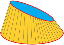
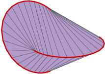
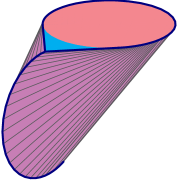
Figure 1. Some convex hulls of two circles.

In the convex hull on the left, the discs of both circles are faces, and every face is exposed. In the oloid in the middle, the discs lie in the interior, an arc of each circle is extreme, and the endpoints of the arcs are nonexposed. In the convex hull on the right, there are two nonexposed stationary bisecants lying on its two-dimensional face, which is the convex hull of one circle and the point where the other circle is tangent to the plane of the first.

These objects have been studied before. Paul Schatz discovered and patented the oloid in 1929 [16], this is the convex hull of two congruent circles in orthogonal planes, each passing through the center of the other. It has found industrial uses [2], and is a well-known toy. A curve in $\mathbb{R}^{3}$ may roll along its edge surface. When rolling, the oloid develops its entire surface and has area equal to that of the sphere [3] with equator one of the circles of the oloid. Other special cases of the convex hull of two circles have been studied from these perspectives [5, 10].

This paper had its origins in Subsection 4.1 of [13], which claimed that the edge surface for a general pair of circles is composed of cylinders. We show that this is only the case when the two circles either meet in two points or are mutually tangent—in all other cases, the edge surface has higher degree and it is an irrational surface of degree eight when the circles are disjoint in $\mathbb{C}\mathbb{P}^{3}$. This is related to Problem 3 on Convexity in [21], on the convex hull of three ellipsoids in $\mathbb{R}^{3}$. An algorithm was presented in [6] (see the video [7]), using projective duality. We sketch this in Section 5, and also apply duality to the convex hull of two circles.

In Section 2, we recall some aspects of convexity and convex algebraic geometry, and show that the convex hull of two circles is the projection of a spectrahedron. We study the edge surface and the edge curve of stationary bisecants of complex conics $C_{1},C_{2}\subset\mathbb{C}\mathbb{P}^{3}$ in Section 3. We show that the edge curve is a reduced curve of bidegree $(2,2)$ in $C_{1}\times C_{2}$ and, if $C_{1}\cap C_{2}=\emptyset$ and neither circle is tangent to the plane of the other, then the edge surface has degree eight. We also classify which curves of bidegree $(2,2)$ arise as edge curves to two conics. All possibilities occur, except a rational curve with a cusp singularity and a maximally reducible curve.

In Section 4, we classify the possible arrangements of two circles lying in different planes in terms that are relevant for their convex hulls. We determine the face lattice and the real edge curve of each type, and show that these convex hulls are spectrahedra only when the circles lie on a quadratic cone.

2. Convex algebraic geometry

We review some fundamental aspects of convexity and convex algebraic geometry, summarize our results about convex hulls of pairs of circles and their edge curves, and show that any such convex hull is the projection of a spectrahedron.

The convex hull of a subset $S\subset\mathbb{R}^{d}$ is

$${\color[rgb]{0,0,1}\operatorname{conv}(S)}\ :=\ \Bigl{\{}\sum_{i=1}^{n}\lambda_{i}s_{i}\mid s_{1},\dotsc,s_{n}\in S\,,\ 0\leq\lambda_{i}\,,\ \mbox{and }1=\sum_{i=1}^{n}\lambda_{i}\Bigr{\}}\,.$$

A set $K$ is convex if it equals its convex hull. A point $p\in K$ is extreme if $K\neq\operatorname{conv}(K\smallsetminus\{p\})$. A compact convex set is the convex hull of its extreme points.

A convex subset $F$ of a convex set $K$ is a face if $F$ contains the endpoints of any line segment in $K$ whose interior meets $F$. A supporting hyperplane $\Pi$ is one that meets $K$ with $K$ lying in one of the half-spaces of $\mathbb{R}^{d}$ defined by $\Pi$. A supporting hyperplane $\Pi$ supports a face $F$ of $K$ if $F\subset K\cap\Pi$, and it exposes $F$ if $F=K\cap\Pi$.

Not all faces of a convex set are exposed. The boundary of the convex hull of two coplanar circles in Fig. 2 consists of one arc on each circle and two bitangent segments. An endpoint $p$ of an arc is not exposed. The only line supporting $p$ is the tangent to the circle at $p$, and this line also supports the adjoining bitangent.

Figure 2. Convex hull of coplanar circles.

A fundamental problem from convex optimization is to describe the faces of a convex set, determining which are exposed, as well as their lattice of inclusions (the face lattice). For more on convex geometry, see [1].

Convex algebraic geometry is the marriage of classical convexity with real algebraic geometry. A real algebraic variety $X$ is an algebraic variety defined over $\mathbb{R}$. If $X$ is irreducible and contains a smooth real point, then its real points are Zariski-dense in $X$, so it is often no loss to consider only the real points. Conversely, many aspects of a real algebraic variety are best understood in terms of its complex points. Studying the complex algebraic geometry aspects of a question from real algebraic geometry is its algebraic relaxation. This relaxation enables the use of powerful techniques from complex algebraic geometry to address the original question.

As the real numbers are ordered, we also consider semialgebraic sets, which are defined by polynomial inequalities. By the Tarski–Seidenberg Theorem on quantifier elimination [19, 22], the class of semialgebraic sets is closed under projections and under images of polynomial maps. A closed semialgebraic set is basic if it is a finite intersection of sets of the form $\{x\mid f(x)\geq 0\}$, for $f$ a polynomial.

Motivating questions about convex algebraic geometry were raised in [15]. A fundamental convex semialgebraic set is the cone of positive semidefinite matrices (the $\operatorname{PSD}$ cone). These are symmetric matrices with nonnegative eigenvalues. The boundary of the $\operatorname{PSD}$ cone is (a connected component of) the determinant hypersurface and every face is exposed. A spectrahedron is an affine section $L\cap\operatorname{PSD}$ of this cone. Write $A{\color[rgb]{0,0,1}\succeq}0$ to indicate that $A\in\operatorname{PSD}$. Parameterizing $L$ shows that a spectrahedron is defined by a linear matrix inequality,

$$\{x\in\mathbb{R}^{m}\mid A_{0}+x_{1}A_{1}+\dotsb+x_{m}A_{m}\succeq 0\}\,,$$

where $A_{0},\dotsc,A_{m}$ are real symmetric matrices.

Images of spectrahedra under linear maps are spectrahedral shadows. Semidefinite programming provides efficient methods to optimize linear objective functions over spectrahedra and their shadows, and a fundamental question is to determine if a given convex semialgebraic set may be realized as a spectrahedron or as a spectrahedral shadow, and to give such a realization. Scheiderer showed that the convex hull of a curve is a spectrahedral shadow [17], and recently showed that there are many convex semialgebraic sets which are not spectrahedra or their shadows [18].

Since the optimizer of a linear objective function lies in the boundary, convex algebraic geometry also seeks to understand the boundary of a convex semialgebraic set. This includes determining its faces and their inclusions, as well as the Zariski closure of the boundary, called the algebraic boundary. This was studied for rational curves [20, 23] and for curves in $\mathbb{R}^{3}$ by Ranestad and Sturmfels [14]. They showed that the algebraic boundary of a space curve $C$ consists of finitely many tritangent planes and a ruled edge surface composed of stationary bisecant lines. A stationary bisecant is a secant $\overline{x,y}$ to $C$ ($x,y\in C$) such that the tangent lines $T_{x}C$ and $T_{y}C$ to $C$ at $x$ and $y$ meet. For a general irreducible space curve of degree $d$ and genus $g$, the edge surface has degree $2(d{-}3)(d{+}g{-}1)$ [11, 14].

For example, suppose that $C$ is a general space quartic (see [11, Rem. 5.5] or [14, Ex. 2.3]). This is the complete intersection of two real quadrics $P$ and $Q$, and has genus one by the adjunction formula [9, Ex. V.1.5.2]. Its edge surface has degree $2(4{-}3)(4{+}1{-}1)=8$ and is the union of four cones. In the pencil of quadrics that contain $C$, $sP+tQ$ for $[s,t]\in\mathbb{P}^{1}$, four are singular and are given by the roots of $\det(sP+tQ)$. Here, the quadratic forms $P,Q$ are expressed as symmetric matrices. Each singular quadric is a cone and each line on that cone is a stationary bisecant of $C$. A general point of $C$ lies on four stationary bisecants, one for each cone.

The union of two circles in different planes is also a space quartic, but it is not in general a complete intersection (the complex points of a complete intersection are connected). We therefore expect a different answer than for general space quartics. We give a taste of that which is to come.

Theorem 2.1.

Let $C_{1}$ and $C_{2}$ be circles in $\mathbb{R}^{3}$ lying in different planes. Their convex hull is a spectrahedron if and only if the scheme $C_{1}\cap C_{2}$ has length 2. When the complex points of the circles are disjoint and neither is tangent to the plane of the other, the edge surface is irreducible and has degree eight. Its rulings are parameterized by a smooth curve of genus one in $C_{1}\times C_{2}$. A general point of $C_{1}\cup C_{2}$ lies on two stationary bisecants.

Proof.

This is proven in Lemma 3.1, and in Theorems 3.3, 3.5 and  4.8. ∎

3. Stationary bisecants to two complex conics

We study stationary bisecants and edge surfaces in the algebraic relaxation of our problem of two circles, replacing circles in $\mathbb{R}^{3}$ by smooth conics in ${\color[rgb]{0,0,1}\mathbb{P}^{3}}=\mathbb{C}\mathbb{P}^{3}$.

A conic $C$ in $\mathbb{P}^{3}$ spans a plane. Let $C_{1}$ and $C_{2}$ be conics spanning different planes, $\Pi_{1}$ and $\Pi_{2}$, respectively. A stationary bisecant is spanned by points $p\in C_{1}$ and $q\in C_{2}$ with $p\neq q$ whose tangent lines $T_{p}C_{1}$ and $T_{q}C_{2}$ meet. Set ${\color[rgb]{0,0,1}\ell}:=\Pi_{1}\cap\Pi_{2}$.

Lemma 3.1.

A point $p\in C_{1}$ lies on two stationary bisecants unless the tangent line $T_{p}C_{1}$ meets $C_{2}$. If the tangent line meets $C_{2}$, then it is the unique stationary bisecant through $p$ unless $p\in C_{2}$ or $T_{p}C_{1}$ lies in the plane $\Pi_{2}$ of $C_{2}$. When $T_{p}C_{1}\subset\Pi_{2}$, the pencil of lines in $\Pi_{2}$ through $p$ are all stationary bisecants.

Proof.

See Fig. 3 for reference.

Figure 3. Stationary bisecants.

Consider the tangent line $T_{p}C_{1}$ for $p\in C_{1}$. Either

$$(i)\ T_{p}C_{1}\ \not\subset\ \Pi_{2}\qquad\mbox{or}\qquad(ii)\ T_{p}C_{1}\ \subset\ \Pi_{2}\,.$$

In case $(i)$, let $q$ be the point where $T_{p}C_{1}$ meets $\Pi_{2}$. There are further cases. When $q\not\in C_{2}$, there are two tangents to $C_{2}$ that meet $q$, and the lines through $p$ and each point of tangency ($r,s$ in Fig. 3) give two stationary bisecants through $p$. If $q\in C_{2}$ and $p\neq q$, then the tangent line $T_{p}C_{1}$ is the only stationary bisecant through $p$.

In case $(ii)$, the tangent line $T_{p}C_{1}$ meets every tangent to $C_{2}$, and every line in $\Pi_{2}$ through $p$ (except $T_{p}C_{2}$ if $p\in C_{2}$) meets $C_{2}$ and is therefore a stationary bisecant. If $p\in C_{2}$, then the tangent line $T_{p}C_{2}$ is a limit of such lines. ∎

Remark 3.2.

When $C_{1}$ is tangent to the plane $\Pi_{2}$ at a point $p$, the pencil of lines in $\Pi_{2}$ through $p$ are degenerate stationary bisecants. When $p\not\in C_{2}$, a general line in the pencil meets $C_{2}$ twice so that the map from $C_{2}$ to this pencil has degree two.

Lines that meet $C_{1}$ and $C_{2}$ in distinct points are given by points $(p,q)\in C_{1}\times C_{2}$ with $p\neq q$. The edge curve $E$ is the Zariski closure of the set of points $(p,q)$ such that $\overline{p,q}$ is a stationary bisecant. As a smooth conic is isomorphic to $\mathbb{P}^{1}$, the edge curve is a curve in $\mathbb{P}^{1}\times\mathbb{P}^{1}$. Subvarieties of products of projective spaces have a multidegree (see [4, § 2]). For a curve $C$ in $\mathbb{P}^{1}\times\mathbb{P}^{1}$, this becomes its bidegree $(a,b)$, where $a$ is the number of points in the intersection of $C$ with $\mathbb{P}^{1}\times\{q\}$ for $q$ general and $b$ the number of points in the intersection of $C$ with $\{p\}\times\mathbb{P}^{1}$ for $p$ general. As $\mathbb{P}^{1}\times\{q\}$ has bidegree $(0,1)$ and $\{p\}\times\mathbb{P}^{1}$ bidegree $(1,0)$, the intersection pairing on curves in $\mathbb{P}^{1}\times\mathbb{P}^{1}$, expressed in terms of bidegree, is

(1) $$(a,b)\cdot(c,d)\ =\ ad+bc\ \in\ \mathbb{Z}\,.$$

A curve of bidegree $(a,b)$ is defined in homogeneous coordinates $([s:t],[u:v])$ for $\mathbb{P}^{1}\times\mathbb{P}^{1}$ by a bihomogeneous polynomial that has degree $a$ in $s,t$ and $b$ in $u,v$.

Theorem 3.3.

The edge curve $E$ has bidegree $(2,2)$.

Proof.

In the projection to $C_{1}$, two points of $E$ map to a general point $p\in C_{1}$, by Lemma 3.1. Thus the intersection number of $E$ with $\{p\}\times C_{2}$ is 2 and vice-versa for $C_{1}\times\{q\}$, for general $q\in C_{2}$. Consequently, $E$ has bidegree $(2,2)$.

We compute the defining equation of $E$ to give a second proof. This begins with a parameterization of the conics. Let $f_{i,0},\dotsc,f_{i,3}\in H^{0}(\mathbb{P}^{1},\mathcal{O}(2))$ for $i=1,2$ be two quadruples of homogeneous quadrics that each span $H^{0}(\mathbb{P}^{1},\mathcal{O}(2))$. Each quadruple gives a map $f_{i}\colon\mathbb{P}^{1}\to\mathbb{P}^{3}$ whose image is a conic $C_{i}$. The plane $\Pi_{i}$ of $C_{i}$ is defined by the linear relation among $f_{i,0},\dotsc,f_{i,3}$, and we assume that $\Pi_{1}\neq\Pi_{2}$.

In coordinates, if $[s:t]\in\mathbb{P}^{1}$, then the image

$$f_{i}[s:t]\ =\ [f_{i,0}(s,t):f_{i,1}(s,t):f_{i,2}(s,t):f_{i,3}(s,t)]\,$$

is the corresponding point of $C_{i}$. Its tangent line is spanned by $\partial_{s}f_{i}$ and $\partial_{t}f_{i}$, where $\partial_{x}:=\frac{\partial}{\partial x}$, as $s\partial_{s}f+t\partial_{t}f=2f$, for a homogeneous quadric $f$. The points $f_{1}[s:t]$ and $f_{2}[u:v]$ span a stationary bisecant when their tangents meet. Equivalently, when

(2) $$E(s,t,u,v)\ :=\ \det\begin{pmatrix}\partial_{s}f_{1,0}&\ \partial_{s}f_{1,1}&\ \partial_{s}f_{1,2}&\ \partial_{s}f_{1,3}\\ \rule{0.0pt}{11.0pt}\partial_{t}f_{1,0}&\ \partial_{t}f_{1,1}&\ \partial_{t}f_{1,2}&\ \partial_{t}f_{1,3}\\ \rule{0.0pt}{11.0pt}\partial_{u}f_{2,0}&\ \partial_{u}f_{2,1}&\ \partial_{u}f_{2,2}&\ \partial_{u}f_{2,3}\\ \rule{0.0pt}{11.0pt}\partial_{v}f_{2,0}&\ \partial_{v}f_{2,1}&\ \partial_{v}f_{2,2}&\ \partial_{v}f_{2,3}\end{pmatrix}\ =\ 0\,.$$

As the first two rows have bidegree $(1,0)$ and the second two have bidegree $(0,1)$, this form $E(s,t,u,v)$ has bidegree $(2,2)$. ∎

Example 3.4.

Suppose that $C_{1}$ and $C_{2}$ are the unlinked unit circles where $C_{1}$ is centered at the origin and lies in the $xy$-plane and $C_{2}$ is centered at $(3,0,0)$ and lies in the $xz$-plane. If we choose homogeneous coordinates $[X_{0}:X_{1}:X_{2}:X_{3}]$ for $\mathbb{P}^{3}$ where $(x,y,z)=\frac{1}{X_{0}}(X_{1},X_{2},X_{3})$, then these admit parametrizations

$$[s:t]\ \longmapsto\ [s^{2}+t^{2}:s^{2}-t^{2}:2st:0]\quad\mbox{and}\quad[u:v]\ \longmapsto\ [u^{2}+v^{2}:2u^{2}+4v^{2}:0:2uv]\,.$$

Dividing the determinant (2) by $-16$ gives the equation for the edge curve $E$,

$$s^{2}u^{2}\ -\ 3s^{2}v^{2}\ -\ 3t^{2}u^{2}\ +\ 5t^{2}v^{2}\,,$$

which is irreducible. We draw $E$ below in the window $|s/t|,|u/v|\leq 5$ in $\mathbb{R}\mathbb{P}^{1}\times\mathbb{R}\mathbb{P}^{1}$.

(3)

The Zariski closure of the union of all stationary bisecants is the ruled edge surface $\mathcal{E}$. By Lemma 3.1, a general point of one of the conics lies on two stationary bisecants. Therefore, each conic is a curve of self-intersections of $\mathcal{E}$, and the multiplicity of $\mathcal{E}$ at a general point of a conic is $2$.

Theorem 3.5.

The edge surface $\mathcal{E}$ has degree eight when $C_{1}\cap C_{2}=\emptyset$ and neither is tangent to the plane of the other.

Proof.

The line $\ell=\Pi_{1}\cap\Pi_{2}$ meets each conic in two points and therefore meets $\mathcal{E}$ in at least four points. Any other point ${\color[rgb]{0,0,1}r}\in\ell\cap\mathcal{E}$ lies on a stationary bisecant $m$ between a point $p$ of $C_{1}$ and a point $q$ of $C_{2}$. As $p,r\in\Pi_{1}$, we have $m\subset\Pi_{1}$, and similarly $m\subset\Pi_{2}$. Thus $m=\ell$, but $\ell$ is not a stationary bisecant, a contradiction.

Each of the four points of $\ell\cap\mathcal{E}$ has multiplicity two on $\mathcal{E}$ by Lemma 3.1 and the observation preceding the statement of the theorem. Thus, $\mathcal{E}$ has degree eight.

We give a second proof. Let $m$ be a general line that meets $\mathcal{E}$ transversally. The points of $m\cap\mathcal{E}$ lie on stationary bisecants that meet $m$. We count these using intersection theory. Let ${\color[rgb]{0,0,1}M}\subset C_{1}\times C_{2}$ be the curve whose points are pairs $(p,q)$ such that the secant line spanned by $p$ and $q$ meets $m$. Stationary bisecants that meet $m$ are points of intersection of $M$ and the edge curve $E$. We compute the bidegree of $M$.

Fix a point $p\in C_{1}$ with $p\not\in\Pi_{2}$. Secant lines through $p$ rule the cone over $C_{2}$ with vertex $p$. As this cone meets $m$ in two points, we have $\deg(M\cap\{p\}\times C_{2})=2$. The symmetric argument with a point of $C_{2}$ shows that $M$ has bidegree $(2,2)$. By (1), $M$ meets $E$ in $(2,2)\cdot(2,2)=4+4=8$ points. This proves the theorem. ∎

The arguments in this proof using intersection theory are similar to arguments used in the contributions [4, 12] in this volume.

Remark 3.6.

Each irreducible component $C$ of the edge curve $E$ gives an algebraic family of stationary bisecants and an irreducible component $\mathcal{C}$ of the edge surface $\mathcal{E}$. If $C$ has bidegree $(a,b)$, then the corresponding component $\mathcal{C}$ of $\mathcal{E}$ has degree at most $(2,2)\cdot(a,b)=2(a+b)$. This is not an equality when the intersection $M\cap E$ has a basepoint or when the general point of $\mathcal{C}$ contains two stationary bisecants. This occurs when one circle is tangent to the plane of the other and there are one or more components of degenerate stationary bisecants.

Example 3.7.

The real points of the edge curve (3) of Example 3.4 had two connected components (the picture showed a patch of $\mathbb{R}\mathbb{P}^{1}\times\mathbb{R}\mathbb{P}^{1}$). Thus, the set of real points of the edge surface has two components. Stationary bisecants corresponding to the oval in the center of (3) lie along the convex hull, which shown on the left below. The others bound a nonconvex set that lies inside the convex hull. We display it in an expanded view on the right below.

            

The planes of the circles meet in the $x$-axis. For sufficiently small $\epsilon>0$, the line defined by $y=z=\epsilon$ meets $\mathcal{E}$ transversally. Near each point of a circle lying on the $x$-axis it meets $\mathcal{E}$ in two points, one for each of the two families of stationary bisecants passing through the nearby arc of the circle. These eight points are real.

A curve of bidegree $(2,2)$ on $\mathbb{P}^{1}\times\mathbb{P}^{1}$ has arithmetic genus one, by the adjunction formula [9, Ex. V.1.5.2]. If smooth, then it is an irrational genus one curve. Another way to see this is that the projection to a $\mathbb{P}^{1}$ factor is two-to-one, except over the branch points, of which there are four, counted with multiplicity. Indeed, writing its defining equation as a quadratic form in the variables $(u,v)$ for the second $\mathbb{P}^{1}$ factor, its coefficients are quadratic forms in the variables $s,t$ of the first $\mathbb{P}^{1}$. The projection to the first has branch points where the discriminant vanishes, which is a quartic form. By elementary topology, a double cover of $\mathbb{C}\mathbb{P}^{1}$ with four branch points has Euler characteristic zero, again implying that it has genus one.

Lemma 3.8.

For every set $S$ of four points of $C_{1}$, there is a conic $C_{2}$ such that the projection to $C_{1}$ of the edge curve is branched over $S$.

Proof.

Let $p$ be the point of intersection of two of the tangents to $C_{1}$ at points of $S$ and $q$ be the point of intersection of the other two tangents (see Fig. 4). Since the tangent $T_{s}C_{1}$ at any point $s\in S$ meets $C_{2}$ (in one of the points $p$ or $q$), Lemma 3.1 implies this is the unique stationary bisecant involving the point $s$. Thus, the points of $S$ are branch points of the projection to $C_{1}$ of the edge curve. ∎

Figure 4. Conic giving specified branch points.

Remark 3.9.

There are three families of conics $C_{2}$ giving an edge curve branched over $S$. These correspond to the three partitions of $S$ into two parts of size two. Each partition determines two points $p,q$ on the plane $\Pi_{1}$ of $C_{1}$ where the tangent lines at the points in each part meet. The corresponding family is the collection of conics $C_{2}$ that meet $\Pi_{1}$ transversally in $p$ and $q$.

If both $C_{1}$ and $S\subset C_{1}$ are real and we choose an affine $\mathbb{R}^{3}$ containing the points $p$ and $q$, then we may choose $C_{2}$ to be a circle.

The isomorphism class of a complex smooth genus one curve is determined by its $j$-invariant [9, § IV.4]. This may be computed from the branch points $S$ of any degree two map to $\mathbb{P}^{1}$. Explicitly, if we choose coordinates on $\mathbb{P}^{1}$ so that the branch points $S$ are $\{0,1,\lambda,\infty\}$, then the $j$-invariant is

$$2^{8}\cdot\frac{(\lambda^{2}-\lambda+1)^{3}}{\lambda^{2}(\lambda-1)^{2}}\,.$$

We have the following corollary of Lemma 3.8.

Theorem 3.10.

For every conic $C_{1}$ and every $J\in\mathbb{C}$, there is a conic $C_{2}$ such that the edge curve has $j$-invariant $J$. When $C_{1}$ and $S\subset C_{1}$ are real, $C_{2}$ may be a circle.

We now classify the possible edge curves $E$ to a pair of conics $C_{1}$ and $C_{2}$ lying in distinct planes $\Pi_{1}$ and $\Pi_{2}$. By Lemma 3.12, every component of $E$ is reduced. If $E=F\cup G$ is reducible, then we have that $(2,2)=\mbox{bidegree}(F)+\mbox{bidegree}(G)$. Thus, the bidegrees of the components of $E$ form a partition of $(2,2)$. If $E$ is irreducible, then either it is smooth of genus one or singular of arithmetic genus one and hence rational. Any curve of bidegree $(1,a)$ or $(a,1)$ is rational. Table 1 gives the different possibilities, along with pictures of a real curve.

smooth (generic)	nodal rational	cuspidal	$2(1,0)+2(0,1)$

$2(1,1)$	$(2,1)+(0,1)$	$(2,1)+(0,1)$	$(1,1)+(0,1)$	$(1,1)+(0,1)$
			$\ \ \ +(1,0)$	$\ \ \ +(1,0)$

Table 1. Types of $(2,2)$-curves.

Theorem 3.11.

All types of $(2,2)$-curves of Table 1 occur as the edge curve of a pair of conics $C_{1},C_{2}$ lying in distinct planes except a curve with a cusp and a reducible curve $2(1,0)+2(0,1)$ with four components.

For existence, see Tables 2, 3 and 4, which display edge curves of two circles in all possible configurations. We rule out edge curves with a cusp and reducible edge curves of type $2(1,0)+2(0,1)$. We first analyze the singularities of edge curves.

Lemma 3.12.

The edge curve $E$ is reduced. A point $(p,q)\in C_{1}\times C_{2}$ is a singular point of $E$ only if $p=q$ or $T_{p}C_{1}\subset\Pi_{2}$ or $T_{q}C_{2}\subset\Pi_{1}$. There are five possibilities for $p,q$ and the tangents, up to interchanging the conics $C_{1}$ and $C_{2}$.

1. $p=q$ and the tangent to each conic at $p$ does not lie in the plane of the other.

2. $p=q$ with $T_{p}C_{1}\subset\Pi_{2}$, but $T_{q}C_{2}\not\subset\Pi_{1}$.

3. $p=q$ with both $T_{p}C_{1}\subset\Pi_{2}$ and $T_{q}C_{2}\subset\Pi_{1}$.

4. $p\neq q$ and $T_{p}C_{1}\subset\Pi_{2}$, but $T_{q}C_{2}\not\subset\Pi_{1}$. Then $p\in T_{q}C_{2}$ is a stationary bisecant.

5. $p\neq q$ and $T_{p}C_{1}=T_{q}C_{2}$ is $\Pi_{1}\cap\Pi_{2}$, and is a stationary bisecant.

Proof.

Let $(p,q)\in C_{1}\times C_{2}$ be a point on a curve $E$ of bidegree $(2,2)$. If the fiber of $E$ in one of the projections from $(p,q)$, say to $C_{2}$, has exactly two points, then $E$ is smooth at $(p,q)$. Indeed, as $E$ is a $(2,2)$ curve, $E\cap(C_{1}\times\{q\})$ is either $C_{1}\times\{q\}$ or one double or two simple points, and if two, then $E$ is smooth at each point.

Consequently, there are three possibilities for points of $E$ in the fibers of the projections to $C_{1}$ and $C_{2}$ containing a singular point $(p,q)$. Either

1. $(p,q)$ is the only point of $E$ in both fibers,

2. $(p,q)$ is the only point in one fiber and the other fiber is a component of $E$, or

3. both fibers are components of $E$.

In Case 2, $E$ has at least one component with either linear bidegree $(1,0)$ or $(0,1)$, and in Case 3, it has at least one component with each linear bidegree.

Now let $E$ be the edge curve, which is smooth at any point $(p,q)$ where there is another point in one of the two fibers of projections to $C_{i}$. Lemma 3.1 implies that there are two points in $E$ over a general point of either conic, so every component of $E$ is smooth at a generic point and therefore $E$ is reduced. By Lemma 3.1 and the analysis above, a point $(p,q)\in E$ is singular if and only if both tangents meet the other conic for otherwise there is a second point in one of the fibers.

If $T_{p}C_{1}\subset\Pi_{2}$, then every line in $\Pi_{2}$ through $p$ is a stationary bisecant, so $E$ contains $\{p\}\times C_{2}$, which has bidegree $(1,0)$. If $T_{q}C_{2}\subset\Pi_{1}$, then as before $E$ contains $C_{1}\times\{q\}$, which has bidegree $(0,1)$. If neither occurs, but $E$ is singular at $(p,q)$, then we are in Case $(i)$. When $p=q$ and we are not in Case $(i)$, then, up to interchanging the indices 1 and 2, we are in either Case $(ii)$ or $(iii)$. When $p\neq q$, so that one circle is tangent to the plane of the other, then we are in either Case $(iv)$ or $(v)$. ∎

of Theorem 3.11.

We need only to rule out that the edge curve $E$ has type $2(1,0)+2(0,1)$ or has a cusp. By Lemma 3.12, $E$ has a component $\{p\}\times C_{2}$ of bidegree $(1,0)$ exactly when $C_{1}$ is tangent to the plane $\Pi_{2}$ at the point $p$. Since $\Pi_{1}\neq\Pi_{2}$, there is at most one such point of tangency on $C_{1}$, so $E$ has at most one component of bidegree $(1,0)$ and the same is true for a component of bidegree $(0,1)$. Thus the type $2(1,0)+2(0,1)$ cannot occur for an edge curve.

We show that if $(p,q)\in E$ is a singular point in Case $(i)$ of Lemma 3.12, then $E$ has a node at $(p,q)$, ruling out a cusp and completing the proof.

Suppose that $p=q$ and the tangents to each conic at $p$ do not lie in the plane of the other. Choose coordinates $x,y,z,w$ for $\mathbb{P}^{3}$ so that $\Pi_{1}$ is the plane $z=0$, $\Pi_{2}$ is the plane $x=0$, $T_{p}C_{1}$ is the line $y=z=0$, $T_{p}C_{2}$ is $x=y=0$, and $p=[0:0:0:1]$. Then we may choose parametrizations near $p$ for $C_{1}$ and $C_{2}$ of the form

(4) $$\begin{array}[]{rcl}C_{1}\ \colon\ s&\longmapsto&[\,s+as^{2}\,:\,bs^{2}\,:\,0\,:\,1+cs+ds^{2}\,]\\ \rule{0.0pt}{12.0pt}C_{2}\ \colon\ u&\longmapsto&[\,0\,:\,\beta u^{2}\,:\,u+\alpha u^{2}\,:\,1+\gamma u+\delta u^{2}\,]\,,\end{array}$$

for some $a,b,c,d,\alpha,\beta,\gamma,\delta\in\mathbb{C}$ where $b\beta\neq 0$. The edge curve is defined by

(5) $$\det\begin{pmatrix}s+as^{2}&bs^{2}&0&1+cs+ds^{2}\\ 1+2as\;&2bs&0&c+2ds\\ 0&\beta u^{2}&u+\alpha u^{2}&\;1+\gamma u+\delta u^{2}\;\\ 0&\;2\beta u\;&\;1+2\alpha u\;&\gamma+2\delta u\end{pmatrix}\\ \rule{0.0pt}{12.0pt}\ =\ \left(\beta(ac-d)-b(\alpha\gamma-\delta)\right)s^{2}u^{2}-2b\alpha s^{2}u+2a\beta su^{2}+\beta u^{2}-bs^{2}\,.$$

Indeed, the matrix has rows $f_{1}(s),f^{\prime}_{1}(s),f_{2}(u),f^{\prime}_{2}(u)$, where $f_{i}$ is the parameterization of $C_{i}$ (4). The determinant vanishes when the tangent to $C_{1}$ at $f_{1}(s)$ meets the tangent to $C_{2}$ at $f_{2}(u)$. The terms of lowest order in (5), $\beta u^{2}-bs^{2}$, have distinct linear factors when $b\beta\neq 0$. Thus $E$ has a node when $s=u=0$, which is $(p,p)$. ∎

4. Convex hull of two circles in $\mathbb{R}^{3}$

We classify the relative positions of two circles in $\mathbb{R}^{3}$ and show that the combinatorial type of the face lattice of their convex hull depends only upon their relative position. This relative position is determined by the combinatorial type of the face lattice and the real geometry of the edge curve. We use this classification to determine when the convex hull of two circles is a spectrahedron.

Let $C_{1},C_{2}$ be circles in $\mathbb{R}^{3}$ lying in distinct planes $\Pi_{1}$ and $\Pi_{2}$, respectively. The intersection $C_{1}\cap\Pi_{2}$ in $\mathbb{C}\mathbb{P}^{3}$ is either two real points, two complex conjugate points, or $C_{1}$ is tangent to $\Pi_{2}$ at a single real point. Let ${\color[rgb]{0,0,1}m_{1}}$ be the number of real points in this intersection, and the same for $m_{2}$. Order the circles so that $m_{1}\geq m_{2}$, and call $[m_{1},m_{2}]$ the intersection type of the pair of circles.

The configuration of the circles is determined by the order of their points along the line ${\color[rgb]{0,0,1}\ell}:=\Pi_{1}\cap\Pi_{2}\subset\mathbb{R}^{3}$. For example, $C_{1}$ and $C_{2}$ have order type $(1,2,1,2)$ along $\ell$ when they have intersection type $[2,2]$ and meet $\ell$ in distinct points which alternate. If $C_{1}\cap C_{2}\neq\emptyset$, then we write $S$ for that shared point. For example, if $C_{1}$ meets $\ell$ in two real points with $C_{2}$ tangent to $\ell$ at one, then this pair has order type $(1,S)$. The intersection type may be recovered from the order type.

A further distinction is necessary for intersection type $[0,0]$, when both circles meet $\ell$ in two complex conjugate points. In $\mathbb{C}\mathbb{P}^{3}$ either $C_{1}\cap C_{2}=\emptyset$ or $C_{1}\cap\ell=C_{2}\cap\ell$. Write $\emptyset$ for the order type in the first case and $(2c)$ in the second. By Lemma 3.12, the edge curve is smooth in order type $\emptyset$ and singular in order type $(2c)$.

Lemma 4.1.

There are fifteen possible order types of two circles in $\mathbb{R}^{3}$.

Proof.

See Tables 2, 3, and 4 for the order types of circles and their convex hulls.

The possible intersection types are $[0,0]$, $[1,0]$, $[1,1]$, $[2,0]$, $[2,1]$, and $[2,2]$. For $[0,0]$, we noted two order types, and intersection types $[1,0]$ and $[2,0]$ each admit one order type, namely $(1)$ and $(1,1)$, respectively.

For $[1,1]$, each circle $C_{i}$ is tangent to $\ell$ at a point $p_{i}$. Either $p_{1}\neq p_{2}$ or $p_{1}=p_{2}$, so there are two order types, $(1,2)$ and $(S)$.

For $[2,1]$, the line $\ell$ is secant to circle $C_{1}$ and $C_{2}$ is tangent to $\ell$ at a point $p_{2}$. Either $p_{2}$ is in the exterior of $C_{1}$ or it lies on $C_{1}$ or it is interior to $C_{1}$. These give three order types $\ell$, $(1,1,2)$, $(1,S)$, and $(1,2,1)$, respectively.

Finally, for $[2,2]$ there are three order types when all four point are distinct, $(1,1,2,2)$, $(1,2,1,2)$, and $(1,2,2,1)$. When one point is shared, we have $(1,2,S)$ or $(1,S,2)$. Finally, both points may be shared, giving $(S,S)$. ∎

$[0,0]$  $\emptyset$	$[2,0]$  $(1,1)$	$[2,2]$  $(1,2,2,1)$
$[2,2]$  $(1,1,2,2)$	$[2,2]$  $(1,2,1,2)$	$[2,2]$  $(1,S,2)$

Table 2. Some convex hulls, intersection and order types, and edge curves.

$[2,2]$  $(1,2,S)$	$[2,2]$  $(S,S)$	$[0,0]$  $(2c)$

Table 3. More convex hulls, intersection and order types, and edge curves.

$[2,1]$  $(1,2,1)$	$[2,1]$  $(1,S)$	$[2,1]$  $(1,1,2)$
$[1,0]$  $(1)$	$[1,1]$  $(1,2)$	$[1,1]$  $(S)$

Table 4. More convex hulls, intersection and order types, and edge curves.

The order type of the circles determines the combinatorial type of the face lattice of their convex hull $K$. Describing the face lattice means identifying all (families of) faces of $K$, their incidence relations, and which are exposed/not exposed. Throughout, $D_{i}$ is the disc of the circle $C_{i}$. We invite the reader to peruse our gallery in Tables 2, 3, and 4 while reading this classification. Our main result is the following.

Theorem 4.2.

The order type of $C_{1},C_{2}$ determines the combinatorial type of the face lattice of $K$, as summarized in Table 5. There are eleven distinct combinatorial types of face lattice. The combinatorial type of the face lattice, together with the real algebraic geometry of its edge curve, determines the order type.

We determine the face lattice for each order type. Some general statements are given in preliminary results which precede our proof of Theorem 4.2. The statements are asymmetric, with the symmetric statement obtained by interchanging 1 and 2. We first study the section ${\color[rgb]{0,0,1}\kappa_{1}}:=K\cap\Pi_{1}$ of $K$, which contains $D_{1}$.

Lemma 4.3.

$\kappa_{1}=\operatorname{conv}(C_{1},C_{2}\cap\Pi_{1})$.

Proof.

As $D_{i}=\operatorname{conv}(C_{i})$, $K=\operatorname{conv}(D_{1},D_{2})$. Therefore a point $x\in K$ is a convex combination $\lambda y+\mu z$ ($\lambda,\mu\geq 0$ with $\lambda+\mu=1$) of points $y\in D_{1}$ and $z\in D_{2}$. If $x\in\kappa_{1}\subset\Pi_{1}$, then as $y\in\Pi_{1}$, we must have that $z\in D_{2}\cap\Pi_{1}=\operatorname{conv}(C_{2}\cap\Pi_{1})$. ∎

Corollary 4.4.

If $C_{2}\cap\Pi_{1}\subset D_{1}$, then we have $\kappa_{1}=D_{1}$. Otherwise, $\kappa_{1}$ is the convex hull of $D_{1}$ and the one or two points of $C_{2}\cap\Pi_{1}$ exterior to $D_{1}$. A point $p\in C_{1}$ is an extreme point of $\kappa_{1}$ if and only if $C_{1}$ and $C_{2}\cap\Pi_{1}$ lie on the same side of $T_{p}C_{1}$. An extreme point $p\in C_{1}$ of $\kappa_{1}$ is not exposed if and only if $T_{p}C_{1}$ meets $C_{2}\smallsetminus\{p\}$. Extreme points of $\kappa_{1}$ are extreme points of $K$ and nonexposed points of $\kappa_{1}$ are nonexposed in $K$. Finally, $\kappa_{1}$ is a face of $K$ if and only if $m_{2}\leq 1$.

Proof.

The first two statements follow from Lemma 4.3. The next two about extreme points $p$ of $\kappa_{1}$ follow as $T_{p}C_{1}$ is the only possible supporting line to $\kappa_{1}$ at $p$. The next, about extreme points of $K$ and its section $\kappa_{1}$, follows by Lemma 4.3, and the last is immediate as $C_{2}$ lies on one side of $\Pi_{1}$ if and only if $|C_{2}\cap\Pi_{1}|<2$. ∎

By Lemma 3.1, a general point $p\in C_{1}$ lies on two stationary bisecants. If $p\in K$ is extreme, then these may support one-dimensional bisecant faces of $K$. We determine the bisecant faces meeting most extreme points. Any plane supporting an extreme point $p\in C_{1}$ contains $T_{p}C_{1}$. If such a plane does not meet $C_{2}$, then $p$ is exposed.

Lemma 4.5.

Let $p\in K$ be an extreme point of $K$. If $T_{p}C_{1}$ neither meets $C_{2}$ nor lies in $\Pi_{2}$, then $p$ is exposed. Such a point $p$ lies on one bisecant face if $m_{2}\leq 1$ and two if $m_{2}=2$. When there are two, one is on each side of $\Pi_{1}$.

Proof.

Let $p\in C_{1}$ be an extreme point of $K$ such that $T_{p}C_{1}$ neither meets $C_{2}$ nor lies in $\Pi_{2}$. By Corollary 4.4, $C_{1}$ and $C_{2}\cap\Pi_{1}$ lie on the same side of $T_{p}C_{1}$ in $\Pi_{1}$. In the pencil $\mathbb{R}\mathbb{P}^{1}$ of planes containing $T_{p}C_{1}$, those meeting $K$ form an interval $I$ containing $\Pi_{1}$ and an interval $\gamma$ of planes meeting $C_{2}$. Each endpoint of $\gamma$ is a plane containing a stationary bisecant through $p$. Our assumptions on $p$ and $T_{p}C_{1}$ imply that $I\neq\mathbb{R}\mathbb{P}^{1}$, so that $p$ is exposed. If $m_{2}\leq 1$, then $\Pi_{1}$ is one endpoint of $I$ and the other is an endpoint of $\gamma$, otherwise the endpoints of $I$ are the endpoints of $\gamma$ and $\Pi_{1}$ is an interior point, which proves the lemma. ∎

Remark 4.6.

Corollary 4.4 identifies the 2-faces, extreme points, and some nonexposed points of $K$. Lemma 4.5 identifies most exposed points and bisecant edges. The rest of the face lattice is determined in the proof of Theorem 4.2. We first understand the boundary of each section $\kappa_{i}=K\cap\Pi_{i}$. Fig. 5 shows the possibilities when $\kappa_{i}$ is not the disc $D_{i}$.

Figure 5. Some possible slices $\kappa_{i}$.

There, $q_{1}$ and $q_{2}$ are points of the other circle on the boundary of $\kappa_{i}$ and points $p_{j}$ are nonexposed points of $C_{i}$ as $T_{p_{j}}C_{i}$ meets $q_{1}$ or $q_{2}$. The line segment between $q_{1}$ and $q_{2}$ is where the disc of the second circle meets $\Pi_{i}$.

of Theorem 4.2.

We give separate arguments for each order type.

Order type $\emptyset$. By Corollary 4.4, both discs are faces of $K$, and every point of the circles is extreme. By Lemma 4.5, all points of the circles are exposed, and each point lies on exactly one bisecant face.

The same description holds for order type $(2c)$. As the edge curve for order type $\emptyset$ is smooth and of genus 1, while that for order type $(2c)$ is singular, the edge curve distinguishes these two order types.

Order type $(1,1)$. Since $m_{1}=2$ and $m_{2}=0$, $D_{1}$ is the only 2-face. The section $\kappa_{2}$ is similar to Fig. 5 (b), so the extreme points on $C_{2}$ form an arc $\wideparen{p_{1},p_{2}}$ whose endpoints are not exposed, each lying on one bisecant edge. The interior points of $\wideparen{p_{1},p_{2}}$ are exposed by Lemma 4.5 and each lies on two bisecant edges. Similarly, every point of $C_{1}$ is exposed and lies on one bisecant edge.

The same description holds for order type $(1,2,1)$. Its edge curve is singular, while order type $(1,1)$ has a smooth edge curve.

Order type $(1,2,2,1)$. Since $m_{1}=m_{2}=2$, $K$ has no 2-faces. Since $C_{2}$ meets the interior of $D_{1}$, Corollary 4.4 implies that every point of $C_{1}$ is extreme and $C_{2}$ has two intervals of extreme points. The four endpoints are not exposed and each lies on one bisecant edge. By Lemma 4.5, every point of $C_{1}$ and of the interior of the arcs on $C_{2}$ is exposed and lies on two bisecant edges.

Order type $(1,1,2,2)$. By Corollary 4.4, $K$ has no 2-faces and each circle has one arc of extreme points, as the sections $\kappa_{i}$ are similar to Fig. 5 (a). As before, each endpoint of an arc is not exposed and lies on one bisecant edge, and each interior point of an arc is exposed and lies on two bisecant edges.

The same description holds for order types $(1,2,1,2)$ and $(1,S,2)$. The edge curve in type $(1,1,2,2)$ has two real components as seen in Example 3.7, while for type $(1,2,1,2)$ there is one real component, and both are smooth. For type $(1,S,2)$, the edge curve is singular at the shared point.

Order type $(1,2,S)$. Again, $K$ has no 2-faces. All points of $C_{1}$ are extreme and $C_{2}$ has an arc of extreme points whose endpoints are not exposed and each lies on one bisecant edge. Also, all interior points of that arc and of $C_{1}$—except possibly the shared point $p$—are exposed and lie on two bisecant edges. The tangents $T_{p}C_{1}$ and $T_{p}C_{2}$ span a plane exposing $p$ and $p$ lies on no bisecant edges.

Order type $(S,S)$. There are no 2-faces and as in type $(1,2,S)$ every point of the circles is extreme, and the nonshared points are exposed and each lies on two bisecant edges. Each shared point is exposed by the plane spanned by the two tangents at that point and neither shared point lies on a bisecant edge.

Order type $(1,S)$. The only 2-face is $D_{1}$. Every point of $C_{1}$ is extreme and $C_{2}$ has an arc $\wideparen{p_{1},p_{2}}$ of extreme points with one endpoint, say $p_{1}$, the shared point where $C_{2}$ is tangent to $\Pi_{1}$. Neither endpoint is exposed and $p_{2}$ lies on one bisecant edge (the bisecant $T_{p_{1}}C_{2}$ meets the interior of $D_{1}$). By Lemma 4.5, every point of $C_{1}$ except $p_{1}$ lies on one bisecant edge and every interior point of $\wideparen{p_{1},p_{2}}$ lies on two bisecant edges, and all of these are exposed.

Order type $(1,1,2)$. The only 2-face is $\kappa_{1}$ and its shape is as in Fig 5 (a) with the vertex $q_{1}$ where $D_{2}$ is tangent to $\Pi_{1}$. There is an arc $\wideparen{p_{1},p_{2}}$ of extreme points of $C_{1}$ whose endpoints are not exposed with each lying on a bisecant edge $\overline{p_{i},q_{1}}$. The section $\kappa_{2}$ has the same shape and $C_{2}$ has an arc $\wideparen{q_{1},q_{2}}$ of extreme points with neither endpoint exposed. The point $q_{2}$ lies on one bisecant edge along $T_{q_{2}}C_{2}$ and $q_{1}$ lies on two bisecant edges $\overline{p_{i},q_{1}}$. Neither of the edges $\overline{p_{i},q_{1}}$ is exposed as $\Pi_{1}$ is the only supporting plane of $K$ containing either edge. Finally, by Lemma 4.5, interior points of the arcs are exposed, with those from $\wideparen{p_{1},p_{2}}$ lying on one bisecant edge and those from $\wideparen{q_{1},q_{2}}$ lying on two.

In the order types of the last row of Table 4, the circle $C_{2}$ is tangent to $\Pi_{1}$ at a point $q_{1}$ and the tangent $T_{q_{1}}C_{2}$ does not meet the interior of $D_{1}$. In the pencil of planes containing $T_{q_{1}}C_{2}$, $\Pi_{1}$ and $\Pi_{2}$ are the endpoints of an interval of planes meeting $K\smallsetminus T_{q_{1}}C_{2}$ and of an interval of planes that meet $K$ only in $T_{q_{1}}C_{2}\cap K$. Thus, both sections $\kappa_{1}$ and $\kappa_{2}$ are 2-faces of $K$ and the face $T_{q_{1}}C_{2}\cap K$ is exposed.

Order type $(1)$. Here, $m_{1}=1$ and $m_{2}=0$. The 2-face $\kappa_{2}$ has the same shape as in order type $(1,1,2)$. The description of the points and bisecant edges meeting $C_{2}$ is also the same. By Lemma 4.5 and the preceding observation, every point of $C_{1}$ is exposed, and all lie on a unique bisecant edge except $q_{1}$, which lies on the two nonexposed bisecant edges $\overline{p_{i},q_{1}}$.

Order type $(1,2)$. This is the most complicated. Each circle is tangent to the plane of the other, sharing a tangent line, and the description is symmetric in the indices $1$ and $2$. The 2-faces are the sections $\kappa_{1}$ and $\kappa_{2}$, with the description for each is nearly the same as for $\kappa_{1}$ in order type $(1,1,2)$. The exception is the bisecant edge $\overline{p_{1},q_{1}}$ lying along the shared tangent. This is exposed, but neither endpoint is exposed. It is also isolated from the other bisecant edges, which form a continuous family.

Order type $(S)$. The two circles are mutually tangent at a point $p$. The 2-faces are $D_{1}$ and $D_{2}$, every point of either circle is extreme, including $p$, and each (except for $p$) lies on one bisecant edge. ∎

Table 5 summarizes the face lattices by order type. In it, when $m_{i}=1$, $p_{i}$ is the point were $C_{i}$ is tangent to the plane of the other circle.

Order Type	0-faces	1-faces	2-faces
$\emptyset$	Points on $C_{1}\cup C_{2}$	One family parameterized by $C_{1}$	$D_{1}$, $D_{2}$
$(1,1)$	Points on $C_{1}$ and points on an arc of $C_{2}$	One family parameterized by $C_{1}$	$D_{1}$
$(1,2,2,1)$	Points on $C_{1}$ and points on two arcs of $C_{2}$	Two families parameterized by $C_{1}$	None
$(1,1,2,2)$	Points on an arc of $C_{1}$
and an arc of $C_{2}$	One family parameterized by a 2-fold branched cover of an arc	None
$(1,2,1,2)$	Same as order type $(1,1,2,2)$
$(1,S,2)$	Same as order type $(1,1,2,2)$
$(1,2,S)$	Points on $C_{1}$ and
an arc of $C_{2}$	Two families parameterized
by $C_{1}\smallsetminus C_{2}$	None
$(S,S)$	Points on $C_{1}\cup C_{2}$	Four families with two parameterized by each arc $C_{1}\smallsetminus C_{2}$	None
$(2c)$	Same as order type $\emptyset$
$(1,S)$	Points on $C_{1}$ and
an arc of $C_{2}$	One family parameterized
by $C_{1}\smallsetminus C_{2}$	$D_{1}$
$(1,1,2)$	Points on an arc of $C_{1}$
and an arc of $C_{2}$	One family parameterized by
the arc of $C_{1}$	$\operatorname{conv}(D_{1},p_{2})$
$(1,2,1)$	Same as order type $(1,1)$
$(1)$	Points on $C_{1}$ and
an arc of $C_{2}$	One family parameterized by
the arc on $C_{2}$	$D_{1}$, $\operatorname{conv}(D_{2},p_{1})$
$(1,2)$	Points on an arc of $C_{1}$
and an arc of $C_{2}$	One family parameterized by either arc, and an isolated bisecant $\overline{p_{1},p_{2}}$	$\operatorname{conv}(D_{1},p_{2})$, $\operatorname{conv}(D_{2},p_{1})$
$(S)$	Points on $C_{1}\cup C_{2}$	One family parameterized by either circle except the common point	$D_{1}$, $D_{2}$

Table 5. Face lattices.

By Theorem 2.1, the convex hull $K$ is a spectrahedral shadow. We use our classification to describe when $K$ is a spectrahedron.

Lemma 4.7.

Let $C_{1},C_{2}\in\mathbb{P}^{3}$ be conics in distinct planes $\Pi_{1}$ and $\Pi_{2}$. If $C_{1}\cap\Pi_{2}=C_{2}\cap\Pi_{1}$, then $C_{1}$ and $C_{2}$ lie on a pencil of quadrics.

Proof.

Since $C_{1},C_{2}$ lie on the singular quadric $\Pi_{1}\cup\Pi_{2}$, we need only find a second quadric containing them. Choose coordinates $[x:y:z:w]$ for $\mathbb{P}^{3}$ so that $\Pi_{1}$ is defined by $w=0$ and $\Pi_{2}$ by $z=0$. Then $C_{1}$ and $C_{2}$ are given by homogeneous quadratic polynomials $f(x,y,z)=0$ and $g(x,y,w)=0$. Since $C_{1}\cap\Pi_{2}=\Pi_{1}\cap C_{2}$, the forms $f(x,y,0)$ and $g(x,y,0)$ define the same scheme, so they are proportional. Scaling $g$ if necessary, we may assume that $f(x,y,0)=g(x,y,0)$. Define ${\color[rgb]{0,0,1}h(x,y,z,w)}$ to be $f(x,y,z)+g(x,y,w)-f(x,y,0)$. It follows that $h(x,y,z,0)=f(x,y,z)$ and $h(x,y,0,w)=g(x,y,w)$, and thus $C_{1}$ and $C_{2}$ lie on the quadric defined by $h$. ∎

Theorem 4.8.

The convex hull of two circles $C_{1}$ and $C_{2}$ lying in distinct planes in $\mathbb{R}^{3}$ is a spectrahedron only if they have order type $(SS)$ or $(2c)$ or $(S)$.

Proof.

We have that $C_{1}\cap\Pi_{2}=C_{2}\cap\Pi_{1}$ in $\mathbb{P}^{3}$ if and only if the circles have order type $(SS)$ or $(2c)$ or $(S)$. By Lemma 4.7, $C_{1}$ and $C_{2}$ lie on a pencil $Q_{1}+tQ_{2}$ of quadrics. Following Example 2.3 in [14], this pencil of quadrics contains singular quadrics given by the real roots of $\det(Q_{1}+tQ_{2})$. Such a singular quadric is given by the determinant of a $2\times 2$ matrix polynomial $Ax+By+Cz+D$, and the block diagonal matrix with blocks $A$, $B$, $C$, and $D$ represents $\operatorname{conv}(C)$ as a spectrahedron.

By Corollary 4.4, $K$ has a nonexposed face when a tangent line to one circle meets the other circle in a different point. This occurs for all the remaining order types of the circles $C_{1}$ and $C_{2}$, except type $\emptyset$ where $C_{1}\cap C_{2}=\emptyset$ in $\mathbb{P}^{3}$. In this case, the edge curve is irreducible with two connected real components and the edge surface meets the interior of $\operatorname{conv}(C)$ (as there are internal stationary bisecants). Thus, $\operatorname{conv}(C)$ is not a basic semialgebraic set and thus not a spectrahedron. ∎

5. Convex hulls through duality

We sketch an alternative approach to studying the convex hull $K$ of two circles that uses projective duality. This is inspired by the paper [6] and accompanying video [7] that explains a solution to the problem of determining the convex hull of three ellipsoids in $\mathbb{R}^{3}$.

Points $\check{\Pi}$ of the dual projective space $\check{\mathbb{P}}^{3}$ correspond to planes $\Pi$ of the primal space $\mathbb{P}^{3}$. A line $\check{\ell}$ represents the pencil of planes containing a fixed line $\ell\subset\mathbb{P}^{3}$, and a plane $\check{o}$ represents the net of planes incident on a point $o\in\mathbb{P}^{3}$. The dual ${\color[rgb]{0,0,1}\check{C}}\subset\check{\mathbb{P}}^{3}$ of a conic $C\subset\mathbb{P}^{3}$ is the set of planes that contain a line tangent to $C$.

Lemma 5.1.

The dual $\check{C}$ to a conic $C$ is a quadratic cone in $\check{\mathbb{P}}^{3}$ with vertex $\check{\Pi}$ corresponding to the plane $\Pi$ of $C$.

Proof.

The pencil of planes containing the tangent line $T_{p}C$ to $C$ is a line lying on $\check{C}$ that meets $\check{\Pi}$ as $T_{p}C\subset\Pi$. Thus, $\check{C}$ is a cone in $\check{\mathbb{P}}^{3}$ with vertex $\check{\Pi}$. Let $o\in\mathbb{P}^{3}$ be any point that is not on $\Pi$. Then the curve $\check{o}\cap\check{C}$ is the set of planes through $o$ that contain a tangent line $T_{p}C$ to $C$. As there are two such planes that contain a general line $\ell$ through $o$—$\ell$ meets two tangents to $C$—the curve $\check{o}\cap\check{C}$ is a conic in $\check{o}$ and $\check{C}$ is the cone over that conic with vertex $\check{\Pi}$. ∎

Let $C_{1},C_{2}$ be circles in $\mathbb{R}^{3}\subset\mathbb{R}\mathbb{P}^{3}$ lying in distinct planes $\Pi_{1},\Pi_{2}$ and let ${\color[rgb]{0,0,1}K}$ be the convex hull of $C_{1}\cup C_{2}$. Let $o$ be any point in the interior of $K$. We will consider the hyperplane $\check{o}\subset\check{\mathbb{R}\mathbb{P}}^{3}$ to be the hyperplane at infinity and set ${\color[rgb]{0,0,1}\check{\mathbb{R}}^{3}}:=\check{\mathbb{R}\mathbb{P}}^{3}\smallsetminus\check{o}$. This is an affine space that contains every hyperplane supporting $K$ as well as all those disjoint from $K$, as every hyperplane incident on $o$ meets the interior of $K$. It also contains the point $\check{\infty}$ corresponding to the hyperplane at infinity in $\mathbb{R}\mathbb{P}^{3}$.

For $i=1,2$, let $\check{C}_{i}$ be the cone in $\check{\mathbb{R}}^{3}$ dual to the conic $C_{i}$. If $o\in\Pi_{i}$, then the vertex $\check{\Pi}_{i}$ of $\check{C}_{i}$ lies at infinity ($\check{\Pi}_{i}\in\check{o}$) and $\check{C}_{i}$ is a cylinder. Neither dual cone contains the point $\check{\infty}$. Let $\check{K}$ be the closure of the component of $\check{\mathbb{R}}^{3}\smallsetminus\check{C}_{1}\smallsetminus\check{C}_{2}$ containing $\check{\infty}$.

Proposition 5.2.

Points $\check{\Pi}$ in the interior of $\check{K}$ are exactly those whose corresponding hyperplane $\Pi$ is disjoint from $K$. Points of the boundary of $\check{K}$ correspond to supporting hyperplanes of $K$, and $\check{K}$ is convex and bounded.

We present an elementary proof of this standard result about convex sets in $\mathbb{R}^{d}$.

Proof.

Choose coordinates $(x,y,z)$ for $\mathbb{R}^{3}$ so that $o=(0,0,0)$ is the origin. An affine hyperplane is defined by the vanishing of an affine form $\Lambda:=ax+by+cz+d$, whose coefficients $[a:b:c:d]$ give homogeneous coordinates for $\check{\mathbb{R}\mathbb{P}}^{3}$. In these coordinates, $\check{\infty}$ is the point $[0:0:0:1]$, $\check{o}$ has equation $d=0$, and the points of the affine $\check{\mathbb{R}}^{3}$ have coordinates $[a:b:c:1]$, so that $\check{\infty}$ is the origin in $\check{\mathbb{R}}^{3}$.

Let $v=(\alpha,\beta,\gamma)\in\mathbb{R}^{3}\smallsetminus\{(0,0,0)\}$ and consider the linear map ${\color[rgb]{0,0,1}\Lambda_{v}}\colon\mathbb{R}^{3}\to\mathbb{R}$,

$$\Lambda_{v}(x,y,z)\ :=\ \alpha x+\beta y+\gamma z\,.$$

Since $\Lambda_{v}^{-1}(0)$ is a plane containing the origin $o$, $\Lambda_{v}(K)$ is a closed interval $[\epsilon,\delta]$ with $0$ in its interior, so that $\epsilon<0<\delta$. Thus, the points

$$\Lambda_{v,t}\ \colon\ [t\alpha:t\beta:t\gamma:1]\ \ \mbox{for}\ \ -\tfrac{1}{\delta}<t<-\tfrac{1}{\epsilon}$$

of $\check{\mathbb{R}\mathbb{P}}^{3}$ are exactly the hyperplanes in $\mathbb{R}\mathbb{P}^{3}$ parallel to $\Lambda_{v}^{-1}(0)$ that are disjoint from $K$ as $\Lambda_{v,t}(K)\subset(0,\infty)$ for $-\tfrac{1}{\delta}<t<-\tfrac{1}{\epsilon}$.

All other planes parallel to $\Lambda^{-1}_{v}(0)$ meet $K$, with $\Lambda_{v,-1/\delta}$ and $\Lambda_{v,-1/\epsilon}$ the hyperplanes in this family that support $K$. These supporting hyperplanes necessarily lie on $\check{C}_{1}\cup\check{C}_{2}$. Hence, the interior of $\check{K}$ is exactly the set of all hyperplanes disjoint from $K$ and its boundary is exactly the set of hyperplanes supporting $K$.

As $o$ lies in the interior of $K$, there is a closed ball centered at $o$ of radius $1/\rho$ contained in the interior of $K$. For any unit vector $v$, the numbers $\epsilon,\delta$ defined by $\Lambda_{v}(K)=[\epsilon,\delta]$ satisfy $|1/\epsilon|,|1/\delta|<\rho$. Thus, the coordinates of points $[\alpha:\beta:\gamma:1]$ in $\check{K}$ satisfy $\|(\alpha,\beta,\gamma)\|<\rho$, proving that $\check{K}$ is bounded.

Let $\Lambda=[a:b:c:1]$ and $\Lambda^{\prime}=[a^{\prime}:b^{\prime}:c^{\prime}:1]$ be points of $\check{K}$. Then $\Lambda(K),\Lambda^{\prime}(K)\subset[0,\infty)$. Since $[0,\infty)$ is convex, for every $t\in[0,1]$, if $\Lambda_{t}:=t\Lambda+(1-t)\Lambda^{\prime}$, then $\Lambda_{t}(K)\subset[0,\infty)$ and so $\Lambda_{t}\in\check{K}$. This proves that $\check{K}$ is convex. ∎

Points in the boundary ($\partial K$) of $\check{K}$ are hyperplanes supporting $K$, and faces of $\check{K}$ correspond to exposed faces of $K$. For example, $\check{\Pi}_{i}\in\partial\check{K}$ if and only if the plane $\Pi_{i}$ of $C_{i}$ supports a two-dimensional face of $K$. Points of the curve in $\partial\check{K}$ where the cones $\check{C}_{1}$ and $\check{C}_{2}$ meet correspond to stationary bisecants, and line segments in the ruling of $\check{C}_{i}$ lying in $\partial\check{K}$ correspond to the exposed points of $C_{i}$ in $K$. This may be seen in Fig. 6,

    

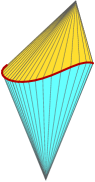
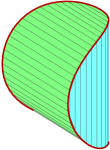
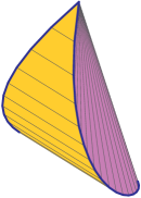
Figure 6. Duals to convex hulls.

which shows the dual bodies to the convex hulls of Fig. 1. For these, the origin $o$ is the midpoint of the segment joining the centers of the circles.

The intersection of two cones on the left has cone points corresponding to the planes of the discs in the boundary of the convex set on the left in Fig. 1. In the center is the dual of the oloid. The origin $o$ is in the interior of the discs of the circles, so both cones $\check{C}_{i}$ are elliptical cylinders. On the right is the intersection of a cone with a horizontal cylinder meeting its vertex. The cylinder is dual to the vertical circle in the rightmost convex set in Fig. 1. The vertex is the 2-dimensional face, and the two branches of the intersection curve at the vertex of the cone have limit the two nonexposed stationary bisecants.

In [6], the authors sketch an exact algorithm (beautifully explained in [7]) to compute the convex hull of three ellipsoids $P$, $Q$, and $R$ in $\mathbb{R}^{3}$. Their approach inspired the previous discussion.

If the origin $o$ lies in the interior of an ellipsoid $P$, then its dual $\check{P}$ is also an ellipsoid. If $o$ lies on $P$, then its dual is a paraboloid and $\check{\infty}$ lies in the convex component of its complement. If $o$ is exterior to $P$, then its dual is a hyperboloid of two sheets, and one of the convex components of its complement contains $\check{\infty}$.

Choosing an origin $o$ in the interior of the convex hull $K$ of $P\cup Q\cup R$ as in Proposition 5.2, $\check{K}$ is a bounded convex set that is the closure of the region in the complement of the duals containing the origin $\check{\infty}$. The video [7] describes the algorithm to compute $K$ when the origin $o$ lies in the interior of all three ellipsoids. In that case, the dual $\check{K}$ of the convex hull of the three ellipsoids is the intersection of the three dual ellipsoids $\check{P}\cap\check{Q}\cap\check{R}$. Computing $\check{K}$ requires the computation of the curves where two dual ellipsoids intersect, and points where three dual ellipsoids meet, and then decomposing the dual ellipsoids along these curves into patches.

This analysis gives three types of points in the boundary of $\check{K}$.

1. Points common to all three dual ellipsoids. These give tritangent planes in $\partial K$.

2. Points on curves given by the pairwise intersection of dual ellipsoids. They are bitangent planes and give bitangent edges. These form 1-dimensional families of 1-faces in $\partial K$.

3. Points on a single dual ellipsoid. These are tangent planes to an ellipsoid at a point of $K$, and give a two-dimensional family of exposed points of $K$ coming from the corresponding ellipsoid.

As we see in Fig. 6, the dual $\check{K}$ eloquently displays information about the exposed faces of $K$, but information about the nonexposed faces is less clear in $\check{K}$.

References

- [1] Alexander Barvinok, A course in convexity, Graduate Studies in Mathematics, vol. 54, American Mathematical Society, Providence, RI, 2002.
- [2] Inversions-Technik GmbH Basle, http://www.oloid.ch/index.php/en/, formerly Oloid AG.
- [3] Hans Dirnböck and Hellmuth Stachel, The development of the oloid, J. Geom. Graph. 1 (1997), no. 2, 105–118.
- [4] Laura Escobar and Allen Knutson, Secants, bitangents, and their congruences, in Combinatorial Algebraic Geometry (eds. G.G. Smith and B. Sturmfels), to appear.
- [5] Steven R. Finch, Convex hull of two orthogonal disks, arxiv.org/1211.4514, 2012.
- [6] Nicola Geismann, Michael Hemmer, and Elmar Schömer, The convex hull of ellipsoids, SCG ’01 Proceedings of the seventeenth annual symposium on Computational geometry, ACM, New York, 2001, pp. 321–322.
- [7] by same author, The convex hull of ellipsoids 2001, https://youtu.be/Tq9OS5iIcBc, 2001.
- [8] Branko Grünbaum, Convex polytopes, second ed., Graduate Texts in Mathematics, vol. 221, Springer-Verlag, New York, 2003, Prepared and with a preface by Volker Kaibel, Victor Klee and Günter M. Ziegler.
- [9] Robin Hartshorne, Algebraic geometry, Springer-Verlag, New York-Heidelberg, 1977, Graduate Texts in Mathematics, No. 52.
- [10] Hiroshi Ira, The development of the two-circle-roller in a numerical way, unpublished note, http://ilabo.bufsiz.jp/, 2011.
- [11] Trygve Johnsen, Plane projections of a smooth space curve, Parameter spaces (Warsaw, 1994), Banach Center Publ., vol. 36, Polish Acad. Sci., Warsaw, 1996, pp. 89–110.
- [12] Kathlén Kohn, Bernt Ivar Utstøl Nødland, and Paolo Tripoli, The multidegree of the multi-image variety, in Combinatorial Algebraic Geometry (eds. G.G. Smith and B. Sturmfels), to appear.
- [13] Kristian Ranestad and Bernd Sturmfels, The convex hull of a variety, Notions of Positivity and the Geometry of Polynomials (Petter Brändén, Mikael Passare, and Mihai Putinar, eds.), Springer, 2011, pp. 331–344.
- [14] by same author, On the convex hull of a space curve, Advances in Geometry 12 (2012), 157–178.
- [15] Raman Sanyal, Frank Sottile, and Bernd Sturmfels, Orbitopes, Mathematika 57 (2011), no. 2, 275–314.
- [16] Paul Schatz, Oloid, a device to generate a tumbling motion, Swiss Patent No. 500,000, 1929.
- [17] Claus Scheiderer, Semidefinite representation for convex hulls of real algebraic curves, arXiv.org/1208.3865, 2012.
- [18] by same author, Semidefinitely representable convex sets, arXiv.org/1617.07048, 2016.
- [19] Abraham Seidenberg, A new decision method for elementary algebra, Ann. of Math. (2) 60 (1954), 365–374.
- [20] Rainer Sinn, Algebraic boundaries of -orbitopes, Discrete Comput. Geom. 50 (2013), no. 1, 219–235.
- [21] Bernd Sturmfels, Fitness, apprenticeship, and polynomials, in Combinatorial Algebraic Geometry, eds. G.G.Smith and B.Sturmfels, to appear.
- [22] Alfred Tarski, A Decision Method for Elementary Algebra and Geometry, RAND Corporation, Santa Monica, Calif., 1948.
- [23] Cynthia Vinzant, Edges of the Barvinok-Novik orbitope, Discrete Comput. Geom. 46 (2011), no. 3, 479–487.
- [24] Günter M. Ziegler, Lectures on polytopes, Graduate Texts in Mathematics, vol. 152, Springer-Verlag, New York, 1995.