Permuted and Augmented Stick-Breaking
Bayesian Multinomial Regression

Abstract

To model categorical response variables given their covariates, we propose a permuted and augmented stick-breaking (paSB) construction that one-to-one maps the observed categories to randomly permuted latent sticks. This new construction transforms multinomial regression into regression analysis of stick-specific binary random variables that are mutually independent given their covariate-dependent stick success probabilities, which are parameterized by the regression coefficients of their corresponding categories. The paSB construction allows transforming an arbitrary cross-entropy-loss binary classifier into a Bayesian multinomial one. Specifically, we parameterize the negative logarithms of the stick failure probabilities with a family of covariate-dependent softplus functions to construct nonparametric Bayesian multinomial softplus regression, and transform Bayesian support vector machine (SVM) into Bayesian multinomial SVM. These Bayesian multinomial regression models are not only capable of providing probability estimates, quantifying uncertainty, increasing robustness, and producing nonlinear classification decision boundaries, but also amenable to posterior simulation. Example results demonstrate their attractive properties and performance.

Keywords: Discrete choice models, logistic regression, nonlinear classification, softplus regression, support vector machines

1 Introduction

Inferring the functional relationship between a categorical response variable and its covariates is a fundamental problem in physical and social sciences. To address this problem, it is common to use either multinomial logistic regression (MLR) (McFadden, 1973; Greene, 2003; Train, 2009) or multinomial probit regression (Albert and Chib, 1993; McCulloch and Rossi, 1994; McCulloch et al., 2000; Imai and van Dyk, 2005), both of which can be expressed as a latent-utility-maximization model that lets an individual make the decision by comparing its random utilities across all categories at once. In this paper, we address the problem via a new stick-breaking construction of the multinomial distribution, which defines a one-to-one random mapping between the category and stick indices. Rather than assuming an individual compares its random utilities across all categories at once, we assume an individual makes a sequence of stick-specific binary random decisions. The choice of the individual is the category mapped to the stick that is the first to choose “1,” or the category mapped to stick $S$ if all the first $S-1$ sticks choose “0.” This framework transforms the problem of regression analysis of categorical variables into the problem of inferring the one-to-one mapping between the category and stick indices, and performing regression analysis of binary stick-specific random variables.

Both MLR and the proposed stick-breaking models link a categorical response variable to its covariate-dependent probability parameters. While MLR is invariant to the permutation of category labels, given a fixed category-stick mapping, the proposed stick-breaking models purposely destruct that invariance. We are motivated to introduce this new framework for discrete choice modeling mainly to facilitate efficient Bayesian inference via data augmentation, introduce nonlinear decision boundaries, and relax a well-recogonized restrictive model assumption of MLR, as described below.

An important motivation is to extend efficient Bayesian inference available to binary regression to multinomial one. In the proposed stick-breaking models, the binary stick-specific random variables of an individual are conditionally independent given their stick-specific covariate-dependent probabilities. Under this setting, one can solve a multinomial regression by solving conditionally independent binary ones. The only requirement is that the underlying binary regression model uses the cross entropy loss. In other words, we require each stick-specific binary random variable to be linked via the Bernoulli distribution to its corresponding stick-specific covariate-dependent probability parameter.

Another important motivation is to improve the model capacity of MLR, which is a linear classifier in the sense that if the total number of categories is $S$, then MLR uses the intersection of $S-1$ linear hyperplanes to separate one class from the others. By choosing nonlinear binary regression models, we are able to enhance the capacities of the proposed stick-breaking models. We are also motivated to relax the independence of irrelevant alternative (IIA) assumption, an inherent property of MLR that requires the probability ratio of any two choices to be independent of the presence or characteristics of any other alternatives (McFadden, 1973; Greene, 2003; Train, 2009). By contrast, the proposed stick-breaking models make the probability ratio of two choices depend on other alternatives, as long as the two sticks that both choices are mapped to are not next to each other.

In light of these considerations, we will first extend the softplus regressions recently proposed in Zhou (2016), a family of cross-entropy-loss binary classifiers that can introduce nonlinear decision boundaries and can recover logistic regression as a special case, to construct Bayesian multinomial softplus regressions (MSRs). We then consider a multinomial generalization of the widely used support vector machine (SVM) (Boser et al., 1992; Cortes and Vapnik, 1995; Schölkopf et al., 1999; Cristianini and Shawe-Taylor, 2000), a max-margin binary classifier that uses the hinge loss. While there has been significant effort in extending binary SVMs into multinomial ones (Crammer and Singer, 2002; Lee et al., 2004; Liu and Yuan, 2011), the resulted extensions typically only provide the predictions of deterministic class labels. By contrast, we extend the Bayesian binary SVMs in Sollich (2002) and Mallick et al. (2005) under the proposed framework to construct Bayesian multinomial SVMs (MSVMs), which naturally provide predictive class probabilities.

We will show that the proposed Bayesian MSRs and MSVMs, which all generalize the stick-breaking construction to perform Bayesian multinomial regression, are not only capable of placing nonlinear decision boundaries between different categories, but also amenable to posterior simulation via data augmentation. Another attractive feature shared by all these proposed Bayesian algorithms is that they can not only predict class probabilities but also quantify model uncertainty. In addition, we will show that robit regression, a robust cross-entropy-loss binary classifier proposed in Liu (2004), can be extended into a robust Bayesian multinomial classifier under the proposed stick-breaking construction.

The remainder of the paper is organized as follows. In Section 2 we briefly review MLR and discuss the restrictions of its stick-breaking construction. In Section 3 we propose the permuted and augmented stick breaking (paSB) to construct Bayesian multi-class classifiers, present the inference, and show how the IIA assumption is relaxed. Under the paSB framework, we show how to transform softplus regressions and support vector machines into Bayesian multinomial regression models in Sections 4 and 5, respectively. We provide experimental results in Section 6 and conclude the paper in Section 7.

2 Multinomial Logistic Regression and Stick Breaking

In this section we first briefly review multinomial logistic regression (MLR). We then use the stick-breaking construction to show how to generate a categorical random variable as a sequence of dependent binary variables, and further discuss a naive approach to transform binary logistic regression under stick breaking into multinomial regression. In the following discussion, we use $i\in\{1,\ldots,N\}$ to index the individual/observation, $s\in\{1,\ldots,S\}$ to index the choice/category, and the prime symbol to denote the transpose operation.

2.1 Multinomial Logistic Regression

MLR that parameterizes the probability of each category given the covariates as

$$\textstyle P(y_{i}=s\,|\,\boldsymbol{x}_{i},\{{\boldsymbol{\beta}}_{s}\}_{1,S})=p_{is},~{}p_{is}={e^{\boldsymbol{x}_{i}^{\prime}{\boldsymbol{\beta}}_{s}}}\big{/}{\big{(}\sum_{j=1}^{S}e^{\boldsymbol{x}_{i}^{\prime}{\boldsymbol{\beta}}_{j}}\big{)}}\vspace{0mm}$$ (1)

is widely used, where $\boldsymbol{x}_{i}\in\mathbb{R}^{P+1}$ consists of $x_{i1}=1$ and $P$ covariates, and ${\boldsymbol{\beta}}_{s}\in\mathbb{R}^{P+1}$ consists of the regression coefficients for the $s$th category (McCullagh and Nelder, 1989; Albert and Chib, 1993; Holmes and Held, 2006). Without loss of generality, one may choose category $S$ as the reference category by setting all the elements of ${\boldsymbol{\beta}}_{S}$ as 0, making $e^{\boldsymbol{x}_{i}^{\prime}{\boldsymbol{\beta}}_{S}}=1$ almost surely (a.s.). For MLR, if data $i$ is assigned to the category with the largest $p_{is}$, then one may consider that category $s$ resides within a convex polytope (Grünbaum, 2013), defined by the set of solutions to $S-1$ inequalities as $\boldsymbol{x}^{\prime}({\boldsymbol{\beta}}_{j}-{\boldsymbol{\beta}}_{s})\leq 0$, where $j\in\{1,\ldots,s-1,s+1,\ldots,S\}$.

Despite its popularity, MLR is a linear classifier in the sense that it uses the intersection of $S-1$ linear hyperplanes to separate one class from the others. As a classical discrete choice model in econometrics, it makes the independence of irrelevant alternatives (IIA) assumption, implying that the unobserved factors for choice making are both uncorrelated and having the same variance across all alternatives (McFadden, 1973; Train, 2009). Moreover, while its log-likelihood is convex and there are efficient iterative algorithms to find the maximum likelihood or maximum a posteriori solutions of ${\boldsymbol{\beta}}_{s}$, the absence of conjugate priors on ${\boldsymbol{\beta}}_{s}$ makes it difficult to derive efficient Bayesian inference. For Bayesian inference, Polson et al. (2013) have introduced the Pólya-Gamma data augmentation for logit models, and combined it with the data augmentation technique of Holmes and Held (2006) for the multinomial likelihood to develop a Gibbs sampling algorithm for MLR. This algorithm, however, has to update ${\boldsymbol{\beta}}_{s}$ one at a time while conditioning on all ${\boldsymbol{\beta}}_{j}$ for $j\neq s$. Thus it may not only lead to slow convergence and mixing, especially when the number of categories $S$ is large, but also prevent us from parallelizing the sampling of $\{{\boldsymbol{\beta}}_{s}\}_{1,S}$ within each MCMC iteration.

2.2 Stick Breaking

Suppose $y_{i}$ is a random variable drawn from a categorical distribution with a finite vector of probability parameters $(p_{i1},\ldots,p_{iS})$, where $S<\infty$, $p_{is}\geq 0$, and $\sum_{s=1}^{S}p_{is}=1$. Instead of directly using $y_{i}\sim\sum_{s=1}^{S}p_{is}\delta_{s}$, one may consider generating $y_{i}$ using the multinomial stick-breaking construction that sequentially draws binary random variables

$$\textstyle{b_{is}\,\big{|}\,\{b_{ij}\}_{j<s}\,\sim\,\mbox{Bernoulli}\left[\left(1-\sum_{j<s}b_{ij}\right)\pi_{is}\right]},~{}~{}\displaystyle\pi_{is}=\frac{p_{is}}{1-\sum_{j<s}p_{ij}}\vspace{0mm}$$ (2)

for $s=1,2,\ldots,S$. Note that $\pi_{iS}=1$ and $b_{iS}=1-\sum_{j=1}^{S-1}b_{ij}$ by construction. Defining $y_{i}=s$ if and only if $b_{is}=1$ and $b_{ij}=0$ for all $j\neq s$, then one has a strick-breaking representation for the multinomial probability parameter as

$$P(y_{i}=s\,|\,\{\pi_{is}\}_{1,S})=P(b_{is}=1)\prod_{j\neq s}P(b_{ij}=0)=\pi_{is}\prod_{j<s}(1-\pi_{ij}),\vspace{0mm}$$ (3)

which, as expected, recovers $p_{is}$ by substituting the definitions of $\pi_{is}$ shown in (2).

The finite stick-breaking construction in (3) can be further generalized to an infinite setting, as widely used in Bayesian nonparametrics (Hjort et al., 2010). For example, the stick-break construction of Sethuraman (1994) represents the length of the $k$th stick using the product of $k$ stick-specific probabilities that are independent, and identically distributed (i.i.d.) beta random variables. It represents a size-biased random permutation of a Dirichlet process (DP) (Ferguson, 1973) random draw, which includes countably infinite atoms whose weights sum to one. The stick-breaking construction of Sethuraman (1994) has also been generalized to represent a draw from a random probability measure that is more general than the DP (Pitman, 1996; Ishwaran and James, 2001; Wang et al., 2011a).

Related to this paper, one may further consider making the stick-specfic probabilities depend on the covariates (Dunson and Park, 2008; Chung and Dunson, 2009; Ren et al., 2011). For example, the logistic stick-breaking process of Ren et al. (2011) uses the product of $k$ covariate-dependent logistic functions to parameterize the probability of the $k$th stick. To implement a stick-breaking process mixture model, truncated stick-breaking representations with a finite number of sticks are commonly used, with inference developed via both Gibbs sampling (Ishwaran and James, 2001; Dunson and Park, 2008; Rodriguez and Dunson, 2011) and variational approximation (Blei and Jordan, 2006; Kurihara et al., 2007; Ren et al., 2011).

Another related work is the order-based dependent Dirichlet processes of Grifin and Steel (2006), which use an ordered stick-breaking construction for mixture modeling, encouraging the data samples close to each other in the covariate space to share similar orders of the sticks and hence similar mixture weights. We will show that the proposed stick-breaking construction is distinct in that all data samples share the same category-stick mapping inferred from the data, with the category labels mapped to lower-indexed sticks subject to fewer geometric constraints on their decision boundaries.

2.3 Logistic Stick Breaking

The stick-breaking construction parameterizes each $p_{is}$ with the product of $s$ probability parameters and links each $y_{i}$ with a unit-norm binary vector $(b_{i1},\ldots,b_{iS})$, where $b_{iy_{i}}=1$ and $b_{ij}=0$ a.s. if $j\neq y_{i}$. Following the logistic stick-breaking construction of Ren et al. (2011), one may represent $p_{is}$ with (3) and parameterize the logit of each $\pi_{is}$ with a latent Gaussian variable $w_{is}$ as $\pi_{is}={e^{w_{is}}}/{\sum_{j=1}^{S}e^{w_{ij}}}$. To model observed or latent multinomial variables, a stick-breaking procedure, closely related to that of Ren et al. (2011), is used in Khan et al. (2012) to transform the modeling of multinomial probability parameters into the modeling of the logits of binomial probability parameters using Gaussian latent variables. As shown in Linderman et al. (2015), this procedure allows using the Pólya-Gamma data augmentation, without requiring the assistance of the technique of Holmes and Held (2006), to construct Gibbs sampling that simultaneously updates all categories in each MCMC iteration, leading to improved performance over the one proposed in Polson et al. (2013).

The simplification brought by the stick-breaking representation, which stochastically arranges its categories in decreasing order, comes with a clear change in that it removes the invariance of the multinomial distribution to label permutation. While the loss of invariance to label permutation may not pose a major issue for Bayesian mixture models inferred with MCMC (Jasra et al., 2005; Kurihara et al., 2007), it appears to be a major obstacle when applying stick breaking for multinomial regression, where the performance is often found to be sensitive to how the labels of the $S$ categories are ordered. In particular, if one constructs a logistic stick breaking model by letting $\mbox{logit}(\pi_{is})=w_{is}=\boldsymbol{x}_{i}^{\prime}{\boldsymbol{\beta}}_{s}$, which means $\pi_{is}=(1+e^{-\boldsymbol{x}_{i}^{\prime}{\boldsymbol{\beta}}_{s}})^{-1}$, then one has

$$\textstyle p_{is}=\big{(}1+e^{-\boldsymbol{x}_{i}^{\prime}{\boldsymbol{\beta}}_{s}}\big{)}^{-1}\prod_{j<s}\big{(}{1+e^{\boldsymbol{x}_{i}^{\prime}{\boldsymbol{\beta}}_{j}}}\big{)}^{-1},\vspace{0mm}$$

which clearly tends to impose fewer geometric constraints on the classification decision boundaries of a category with a smaller $s$. For example, $p_{i1}=\big{(}1+e^{-\boldsymbol{x}_{i}^{\prime}{\boldsymbol{\beta}}_{1}}\big{)}^{-1}$ is larger than $50\%$ if $\boldsymbol{x}_{i}^{\prime}{\boldsymbol{\beta}}_{1}>0$ while $p_{i2}=\big{(}1+e^{\boldsymbol{x}_{i}^{\prime}{\boldsymbol{\beta}}_{1}}\big{)}^{-1}\big{(}1+e^{-\boldsymbol{x}_{i}^{\prime}{\boldsymbol{\beta}}_{2}}\big{)}^{-1}$ is possible to be larger than $50\%$ only if both $\boldsymbol{x}_{i}^{\prime}{\boldsymbol{\beta}}_{1}<0$ and $\boldsymbol{x}_{i}^{\prime}{\boldsymbol{\beta}}_{2}>0$. We will use an example to illustrate this type of geometric constraints in Section 6.1.

Under the logistic stick-breaking construction, not only could the performance be sensitive to how the $S$ different categories are ordered, but the imposed geometric constraints could also be overly restrictive even if the categories are appropriately ordered. Below we address the first issue by introducing a permuted and augmented stick-breaking representation for a multinomial model, and the second issue by adding the ability to model nonlinearity.

3 Permuted and Augmented Stick Breaking

To turn the seemingly undesirable sensitivity of the stick-breaking construction to label permutation into a favorable model property, when label asymmetry is desired, and mitigate performance degradation, when label symmetry is desired, we introduce a permuted and augmented stick-breaking (paSB) construction for a multinomial distribution, making it straightforward to extend an arbitrary binary classifier with cross entropy loss into a Bayesian multinomial one. The paSB construction infers a one-to-one mapping between the labels of the $S$ categories and the indices of the $S$ latent sticks, transforming the problem from modeling a multinomial random variable into modeling $S$ conditionally independent binary ones. It not only allows for parallel computation within each MCMC iteration, but also improves the mixing of MCMC in comparison to the one used in Polson et al. (2013), which updates one regression-coefficient vector conditioning on all the others, as will be shown in Section 6.5. Note that the number of distinct one-to-one label-stick mappings is $S!$, which quickly becomes too large to exhaustively search for the best mapping as $S$ increases. Our experiments will show that the proposed MCMC algorithm can quickly escape from a purposely poorly initialized mapping and subsequently switch between many different mappings that all lead to similar performance, suggesting an effective search space that is considerably smaller than $S!$.

3.1 Category-Stick Mapping and Data Augmentation

The proposed paSB construction randomly maps a category to one and only one of the $S$ latent sticks and makes the augmented Bernoulli random variables $\{b_{is}\}_{1,S}$ conditionally independent to each other given $\{\pi_{is}\}_{1,S}$. Denote $\boldsymbol{z}=(z_{1},\ldots,z_{S})$ as a permutation of $(1,\ldots,S)$, where $z_{s}\in\{1,\ldots,S\}$ is the index of the stick that category $s$ is mapped to. Given the label-stick mapping $\boldsymbol{z}$, let us denote $p_{is}(\boldsymbol{z})$ as the multinomial probability of category $s$, and $\pi_{iz_{s}}(\boldsymbol{x}_{i},{\boldsymbol{\beta}}_{s})$ as the covariate-dependent stick probability that is associated with the covariates of observation $i$ and the stick that category $s$ is mapped to. For notational convenience, we will write $\pi_{iz_{s}}(\boldsymbol{x}_{i},{\boldsymbol{\beta}}_{s})$ as $\pi_{iz_{s}}$ and $\pi_{ij}(\boldsymbol{x}_{i},{\boldsymbol{\beta}}_{s:z_{s}=j})$ as $\pi_{ij}$. We emphasize that here the $s$th regression-coefficient vector ${\boldsymbol{\beta}}_{s}$ is always associated with both category $s$ and the corresponding stick probabily $\pi_{iz_{s}}$, a construction that will facilitate the inference of the label-stick mapping $\boldsymbol{z}$. The following Theorem shows how to generate a categorical random variable of $S$ categories with a set of $S$ conditionally independent Bernoulli random variables. This is key to transforming the problem from solving multinomial regression into solving $S$ binary regressions independently.

Theorem 1

Suppose $y_{i}\sim\sum_{s=1}^{S}p_{is}(\boldsymbol{z})\delta_{s}$, where $[p_{i1}(\boldsymbol{z}),\ldots,p_{iS}(\boldsymbol{z})]$ is a multinomial probability vector whose elements are constructed as

$$p_{is}(\boldsymbol{z})=(\pi_{iz_{s}})^{\mathbf{1}(z_{s}\neq S)}\prod_{j<z_{s}}(1-\pi_{ij}),\textstyle$$ (4)

then $y_{i}$ can be equivalently generated under the permuted and augmented stick-breaking (paSB) construction as

$$y_{i}\sim\sum_{s=1}^{S} \left\{\textstyle\left[\mathbf{1}(b_{iz_{s}}=1)\right]^{\mathbf{1}(z_{s}\neq S)}\prod_{j<z_{s}}\mathbf{1}(b_{ij}=0)\right\}\delta_{s}\,,$$ (5)

$$b_{ij} \sim\emph{\mbox{Bernoulli}}(\pi_{ij}),~{}~{}j\in\{1,\ldots,S\}.$$ (6)

Distinct from the conventional stick breaking in (2) that maps category $s$ to stick $s$ and makes $b_{is}$ depend on $b_{ij},j=1,\ldots,s-1$, under the new construction in (5)-(6), the $S$ categories are now randomly permuted and then one-to-one mapped to $S$ sticks, and the augmented binary random variables $\{b_{ij}\}_{j}$ become mutually independent given $\{\pi_{ij}\}_{j}$. Given $y_{i}$, we still have $b_{ij}=0$ for $j<z_{y_{i}}$ and $b_{iz_{y_{i}}}=1$ a.s., but impose no restriction on any $b_{ij}$ for $j>z_{y_{i}}$, whose conditional posteriors given $y_{i}$ and $\pi_{ij}$ remain the same as their priors. These changes are key to appropriately ordering the latent sticks, more flexibly parameterizing $\pi_{iz_{s}}$ and hence $p_{is}(\boldsymbol{z})$, and maintaining tractable inference.

With paSB, the problem of inferring the functional relationship between the categorical response $y_{i}$ and the corresponding covariates $\boldsymbol{x}_{i}$ is now transformed into the problem of modeling $S$ conditionally independent binary regressions as

$$b_{iz_{s}}\,|\,\boldsymbol{x}_{i},{\boldsymbol{\beta}}_{s}\sim\mbox{Bernoulli}[\pi_{iz_{s}}(\boldsymbol{x}_{i},{\boldsymbol{\beta}}_{s})],~{}i=1,\ldots,N,~{}s=1,\ldots,S.$$

Note that the only requirement for the binary regression model under paSB is that it uses the Bernoulli likelihood. In other words, it uses the cross entropy loss (Murphy, 2012) as

$$-\sum_{i=1}^{N}\ln P(b_{iz_{s}}\,|\,\boldsymbol{x}_{i},{\boldsymbol{\beta}}_{s})=\sum_{i=1}^{N}\big{\{}-b_{iz_{s}}\ln\pi_{iz_{s}}(\boldsymbol{x}_{i},{\boldsymbol{\beta}}_{s})-(1-b_{iz_{s}})\ln[1-\pi_{iz_{s}}(\boldsymbol{x}_{i},{\boldsymbol{\beta}}_{s})]\big{\}}.$$

A basic choice is paSB logistic regression that lets

$$\pi_{iz_{s}}(\boldsymbol{x}_{i},{\boldsymbol{\beta}}_{s})=1/(1+e^{-\boldsymbol{x}_{i}{\boldsymbol{\beta}}_{s}}),$$

which becomes the same as the logistic stick breaking construction described in Section 2.3 if $z_{s}=s$ for all $s\in\{1,\ldots,S\}$. Another choice is paSB-robit regression that extends robit regression of Liu (2004), a robust binary classifier using cross entropy loss, into a robust Bayesian multinomial classifier. In robit regression, observation $i$ is labeled as 1 if $\boldsymbol{x}_{i}^{\prime}{\boldsymbol{\beta}}+\varepsilon_{i}>0$ and as 0 otherwise, where $\varepsilon_{i}$ are independently drawn from a $t$-distribution with $\kappa$ degrees of freedom, denoted as $\varepsilon_{i}\overset{iid}{\sim}t_{\kappa}$. Consequently, the conditional class probability function of robit regression is $P(y_{i}=1\,|\,\boldsymbol{x}_{i},{\boldsymbol{\beta}})=F_{\kappa}(\boldsymbol{x}_{i}^{\prime}{\boldsymbol{\beta}})$, where $F_{\kappa}$ is the cumulative density function of $t_{\kappa}$. The robustness is attributed to the heavy-tail property of $F_{\kappa}(\boldsymbol{x}_{i}^{\prime}{\boldsymbol{\beta}})$, which, if $\kappa<7$, imposes less penalty than the conditional class probability function of logistic regression does on misclassified observations that are far from the decision boundary. Applying Theorem 1, the category probability of paSB-robit regression with $\kappa$ degrees of freedom is shown in (4), where $\pi_{iz_{s}}(\boldsymbol{x}_{i},{\boldsymbol{\beta}}_{s})=F_{\kappa}(\boldsymbol{x}_{i}^{\prime}{\boldsymbol{\beta}}_{s})$. The paSB-robit regression provides a simple solution to robust multiclass classification; with $\{b_{ij}\}_{i,j}$ defined in Theorem 1, we run independent binary robit regressions using the Gibbs sampler proposed in Liu (2004).

In addition to paSB, we define permuted and augmented reverse stick breaking (parSB) in the following Corollary.

Corollary 2

Suppose $y_{i}\sim\sum_{s=1}^{S}p_{is}\delta_{s}$ and

$$p_{is}(\boldsymbol{z})=\textstyle(1-\pi_{iz_{s}})^{\mathbf{1}(z_{s}\neq S)}\prod_{j<z_{s}}\pi_{ij}\,,$$

then $y_{i}$ can also be generated under the permuted and augmented reverse stick-breaking (parSB) representation as

$$\vspace{-3mm}y_{i}\sim\sum_{s=1}^{S} \left\{\textstyle\left[\mathbf{1}(b_{iz_{s}}=0)\right]^{\mathbf{1}(z_{s}\neq S)}\prod_{j<z_{s}}\mathbf{1}(b_{ij}=1)\right\}\delta_{s}\,,$$ (7)

$$b_{ij} \sim\emph{\mbox{Bernoulli}}(\pi_{ij}),~{}~{}j\in\{1,\ldots,S\}.$$

Generally speaking, if $\pi_{iz_{s}}(\boldsymbol{x}_{i},-{\boldsymbol{\beta}}_{s})=1-\pi_{iz_{s}}(\boldsymbol{x}_{i},{\boldsymbol{\beta}}_{s})$, which is the case for logistic stick breaking and robit stick breaking, where $\pi_{iz_{s}}$ are defined as $(1+e^{-\boldsymbol{x}_{i}^{\prime}{\boldsymbol{\beta}}_{s}})^{-1}$ and $F_{\kappa}(\boldsymbol{x}_{i}^{\prime}{\boldsymbol{\beta}}_{s})$, respectively, and Bayesian multinomial SVMs to be discussed in Section 5, then there is no need to introduce parSB as an addition to paSB. Otherwise, there are potential benefits, such as for softplus regressions to be introduced in Section 4, to combine parSB with paSB.

3.2 Inference of Stick Variables and Category-Stick Mapping

Below we first describe Gibbs sampling for the augmented stick variables $\{b_{ij}\}_{1,S}$, and then introduce a Metropolis-Hastings (MH) step to infer the category-stick mapping $\boldsymbol{z}$. Given the category label $y_{i}$, stick probability $\pi_{ij}$, and $\boldsymbol{z}$, we sample $b_{ij}$ as

$$(b_{ij}\,|\,y_{i},\pi_{ij},\boldsymbol{z})\sim\mathbf{1}(j=z_{y_{i}})+\mathbf{1}(j>z_{y_{i}})\mbox{Bernoulli}(\pi_{ij}),\vspace{0mm}$$

for $j=1,\ldots,S-1$, and let

$$b_{iS}=\mathbf{1}(z_{y_{i}}=S).\vspace{0mm}$$

This means we let $b_{ij}=0$ if ${j}<z_{y_{i}}$, $b_{ij}=1$ if $j=z_{y_{i}}$, draw $b_{ij}$ from $\mbox{Bernoulli}(\pi_{ij})$ if $z_{y_{i}}<j<S$, and let $b_{iS}=1$ if and only if $z_{y_{i}}=S$. Note that stick $S$ is used as a reference stick and $\pi_{iS}$ is not used in defining $p_{is}(\boldsymbol{z})$ in (4). Despite having no impact on computing $\{p_{is}\}_{1,S}$, we infer $\pi_{iS}$ ($i.e.$, sample the regression-coefficient vector ${\boldsymbol{\beta}}_{s^{\prime}:z_{s^{\prime}}=S}$) under the likelihood $\prod_{i=1}^{N}\mbox{Bernoulli}(b_{iS};\pi_{iS})$ and use it in a Metropolis-Hastings step, as described in (8) shown below, to decide whether to switch the mappings of two different categories, if one of which is mapped to the reference stick $S$. Once we have an MCMC sample of $\{b_{ij}\}_{1,S}$, we then essentially solve independently $S$ binary classification problems, the $j$th of which can be expressed as $b_{ij}\,|\,\boldsymbol{x}_{i},{\boldsymbol{\beta}}_{s:z_{s}=j}\sim\mbox{Bernoulli}[\pi_{ij}(\boldsymbol{x}_{i},{\boldsymbol{\beta}}_{s:z_{s}=j})].$

Analogously, for parSB, $\{b_{ij}\}_{1,S}$ can be sampled as $(b_{ij}\,|\,y_{i},\pi_{ij},\boldsymbol{z})\sim\mathbf{1}(j<z_{y_{i}})+\mathbf{1}(j>z_{y_{i}})\mbox{Bernoulli}(\pi_{ij})$ for $j=1,\ldots,S-1$, and $b_{iS}=1-\mathbf{1}(z_{y_{i}}=S),$ which means we let $b_{ij}=1$ if ${j}<z_{y_{i}}$, let $b_{ij}=0$ if $j=z_{y_{i}}$, draw $b_{ij}$ from $\mbox{Bernoulli}(\pi_{ij})$ if $z_{y_{i}}<j<S$, and let $b_{iS}=0$ if and only if $z_{y_{i}}=S$.

Since stick-breaking multinomial classification is not invariant to the permutation of its class labels, it may perform substantially worse than it could be if the inherent geometric constraints implied by the current ordering of the labels make it difficult to adapt the decision boundaries to the data. Our solution to this problem is to infer the one-to-one mapping between the category labels and stick indices from the data. We construct a Metropolis-Hastings (MH) step within each Gibbs sampling iteration, with a proposal of switching two sticks that categories $c$ and $c^{\prime}$, $1\leq c<c^{\prime}\leq S$, are mapped to, by changing the current category-stick one-to-one mapping from $\boldsymbol{z}=(z_{1},\ldots,z_{c},\ldots,z_{c^{\prime}},\ldots,z_{S})$ to $\boldsymbol{z}^{\prime}=(z^{\prime}_{1},\ldots,z^{\prime}_{S}):=(z_{1},\ldots,z_{c^{\prime}},\ldots,z_{c},\ldots,z_{S})$. Assuming a uniform prior on $\boldsymbol{z}$ and proposing $(c,c^{\prime})$ uniformly at random from one of the $\binom{S}{2}=S(S-1)/2$ possibilities, we would accept the proposal with probability

$$\small\!\!\!\min\left\{\prod_{i}\frac{\prod_{s=1}^{S}[p_{is}(\boldsymbol{z}^{\prime})]^{\mathbf{1}(y_{i}=s)}}{\prod_{s=1}^{S}[p_{is}(\boldsymbol{z})]^{\mathbf{1}(y_{i}=s)}},~{}1\right\}=\min\left\{\prod_{i}\frac{\prod_{s=1}^{S}\left[(\pi_{iz^{\prime}_{s}})^{\mathbf{1}(z^{\prime}_{s}\neq S)}\prod_{j<z^{\prime}_{s}}(1-\pi_{ij})\right]^{\mathbf{1}(y_{i}=s)}}{\prod_{s=1}^{S}\left[(\pi_{iz_{s}})^{\mathbf{1}(z_{s}\neq S)}\prod_{j<z_{s}}(1-\pi_{ij})\right]^{\mathbf{1}(y_{i}=s)}},~{}1\right\}.\vspace{0mm}$$ (8)

3.3 Sequential Decision Making

Random utility models, including both the logit and probit models as special examples, are widely used to infer the functional relationship between a categorical response variable and its covariates. For discrete choice analysis in econometrics (Hanemann, 1984; Greene, 2003; Train, 2009), these models assume that among a set of $S$ alternatives, an individual makes the choice that maximizes his/her utility $U_{is}=V_{is}+\varepsilon_{is}$, where $V_{is}$ and $\varepsilon_{is}$ represent the observable and unobservable parts of $U_{is}$, respectively. If $V_{is}$ is set as $V_{is}=\boldsymbol{x}_{i}^{\prime}{\boldsymbol{\beta}}_{s}$, then marginalizing out $\boldsymbol{\varepsilon}_{i}=(\varepsilon_{i1},\ldots,\varepsilon_{iS})^{\prime}$ leads to MLR if all $\varepsilon_{is}$ follow the extreme value distribution (McFadden, 1973; Greene, 2003; Train, 2009), and multinomial probit regression if all $\boldsymbol{\varepsilon}_{i}$ follow a multivariate normal distribution (Albert and Chib, 1993; McCulloch and Rossi, 1994; McCulloch et al., 2000; Imai and van Dyk, 2005).

Instead of examining the utilities of all choices before making the decision, the paSB construction is characterized by a sequential decision making process, described as follows. In step one, an individual decides whether to select the choice mapped to stick 1, or to select a choice among the remaining alternatives, $i.e.$, choices $\{s:z_{s}\in\{2,\ldots,S\}\}$. If the individual selects the choice mapped to stick $1$, then the sequential process is terminated. Otherwise this choice is eliminated and the individual proceeds to step two, in which he/she would follow the same procedure to either select the choice mapped to stick $2$ or proceed to the next step to select a choice among the remaining alternatives, $i.e.$, choices $\{s:z_{s}\in\{3,\ldots,S\}\}$. The individual, reconsidering none of the eliminated choices, will keep making a one-vs-remaining decision at each step until the termination of the sequential decision making process.

This unique sequential decision making procedure relaxes the independence of irrelevant alternatives (IIA) assumption, as described in the following Lemma.

Lemma 3

Under the paSB construction, the probability ratio of two choices are influenced by the success probabilities of the sticks that lie between these two choices’ corresponding sticks. In other words, the probability ratio of two choices will be influenced by some other choices if they are not mapped to adjacent sticks.

As in Lemma 3, the paSB construction could adjust how two choices’ probability ratio depends on the other alternatives by controlling the distance between the two sticks that they are mapped to, and hence provide a unique way to relax the IIA assumption. While the widely used MLR can be considered as a random-utility-maximization model with the IIA assumption, the paSB multinomial logistic model performs sequential random utility maximization that relaxes this assumption, as described in Lemma 5 in the Appendix.

4 Bayesian Multinomial Softplus Regression

Logistic regression is a cross-entropy-loss binary classifier that can be straightforwardly extended to paSB multinomial logistic regression (paSB-MLR). However, it is a linear classifier that uses a single hyperplane to separate one class from the other. To introduce nonlinear classification decision boundaries, we consider extending softplus regression of Zhou (2016), a multi-hyperplane binary classifier that uses the cross entropy loss, into multinomial softplus regression (MSR) under paSB.

Softplus regression uses the interaction of multiple hyperplanes to construct a union of convex-polytope-like confined spaces to enclose the data labeled as “1,” which are hence separated from the data labeled as “0”. It is constructed under a Bernoulli-Poisson link (Zhou, 2015) that thresholds at one a latent Poisson count, with the distribution of the Poisson rate defined as the convolution of the probability density functions of $K$ experts, each of which corresponds to the stack of $T$ gamma distributions with covariate-dependent scale parameters. The number of experts $K$ and the number of layers $T$ can be considered as the two model parameters that determine the nonlinear capacity of the model. More specifically, for expert $k$, denoting $r_{k}$ as its weight and ${\boldsymbol{\beta}}_{k}^{t+1}$ as its $t$th regression-coefficient vector, the conditional class probability can be expressed as

$$P(y_{i}=1\,|\,\boldsymbol{x}_{i},\{r_{k},\{{\boldsymbol{\beta}}_{k}^{(t+1)}\}_{1,T}\}_{1,K})=1-\prod_{k=1}^{K}(1-p_{ik}),$$

$$p_{ik}=1-\left(\!1\!+\!e^{\boldsymbol{x}_{i}^{\prime}{\boldsymbol{\beta}}_{k}^{({T}\!+\!1)}}\ln\!\left\{1\!+\!e^{\boldsymbol{x}_{i}^{\prime}{\boldsymbol{\beta}}_{k}^{({T})}}\ln\left[1\!+\!\ldots\ln\left(1\!+\!e^{\boldsymbol{x}_{i}^{\prime}{\boldsymbol{\beta}}_{k}^{(2)}}\right)\right]\right\}\right)^{-r_{k}};$$

when $K=T=1$, the conditional class probability reduces to

$$P(y_{i}=1\,|\,\boldsymbol{x}_{i},r,{\boldsymbol{\beta}})=1-\left(\frac{1}{1+e^{\boldsymbol{x}_{i}^{\prime}{\boldsymbol{\beta}}}}\right)^{r};\vspace{0mm}$$

and when $K=T=r=1$, it becomes the same as that of binary logistic regression. Note that a gamma process, a random draw from which is expressed as $G=\sum_{k=1}^{\infty}r_{k}\delta_{\{{\boldsymbol{\beta}}_{k}^{t+1}\}_{1,T}}$, can be used to support a potentially countably infinite number of experts for softplus regression. For this reason, one can set $K$ as large as permitted by computation and relies on the gamma process’s inherent shrinkage mechanism to turn off unneeded model capacity (not all $K$ experts will be used if $K$ is set to be sufficiently large).

4.1 paSB and parSB Extensions of Softplus Regressions

We first follow Zhou (2016) to define

$$\varsigma(x_{1},\ldots,x_{t})=\ln\left(1+e^{x_{t}}\ln\left\{1+e^{x_{t-1}}\ln\left[1+\ldots\ln\left(1+e^{x_{1}}\right)\right]\right\}\right)\vspace{0mm}$$

as the stack-softplus function. Note that if $t=1$, the stack-softplus function reduces to softplus function $\varsigma(x)=\ln(1+e^{x})$, which is often considered as a smoothed version of the rectifier function, expressed as $\mbox{rectifier}(x)=\max(0,x)$, that has become the dominant nonlinear activation function for deep neural networks (Nair and Hinton, 2010; Glorot et al., 2011; Krizhevsky et al., 2012; LeCun et al., 2015). We then parameterize $\lambda_{iz_{s}}=-\ln(1-\pi_{iz_{s}})$, the negative logarithms of the failure probabilities of the stick that category $s$ is mapped to, as

$$\lambda_{iz_{s}}=\sum_{k=1}^{\infty}r_{sk}\,\varsigma\big{(}\boldsymbol{x}^{\prime}{\boldsymbol{\beta}}_{sk}^{(2)},\ldots,\boldsymbol{x}^{\prime}{\boldsymbol{\beta}}_{sk}^{(T+1)}\big{)},\vspace{0mm}$$ (9)

where the countably infinite atoms $({\boldsymbol{\beta}}_{sk}^{(2)},\ldots,{\boldsymbol{\beta}}_{sk}^{(T+1)})$ and their weights $\{r_{sk}\}_{k}$ constitute a draw from a gamma process $G_{s}\sim\mbox{GaP}(G_{0},1/c_{s})$ (Ferguson, 1973), with $G_{0}$ as a finite and continuous base distribution over a complete separable metric space $\Omega$ and $1/c_{s}$ as a scale parameter. In other words, we let $b_{iz_{s}}\sim\mbox{Bernoulli}(\pi_{iz_{s}})$ or

$$b_{iz_{s}}\sim{\mbox{Bernoulli}}\left[1-\prod_{k=1}^{\infty}\left(\!1\!+\!e^{\boldsymbol{x}_{i}^{\prime}{\boldsymbol{\beta}}_{sk}^{({T}\!+\!1)}}\ln\!\left\{1\!+\!e^{\boldsymbol{x}_{i}^{\prime}{\boldsymbol{\beta}}_{sk}^{({T})}}\ln\left[1\!+\!\ldots\ln\left(1\!+\!e^{\boldsymbol{x}_{i}^{\prime}{\boldsymbol{\beta}}_{sk}^{(2)}}\right)\right]\right\}\right)^{-r_{sk}}~{}\!\right].$$ (10)

As shown in Theorem 10 of Zhou (2016), $b_{iz_{s}}$ can be equivalently generated from a hierarchical model that convolves countably infinite stacked gamma distributions, with covariate-dependent scales, as

$$~{}~{}~{}~{}~{}\theta^{({T})}_{isk}\sim{\mbox{Gamma}}\left(r_{sk},e^{\boldsymbol{x}_{i}^{\prime}{\boldsymbol{\beta}}^{({T}+1)}_{sk}}\right),$$

$$~{}~{}~{}~{}~{}~{}~{}~{}~{}~{}~{}~{}~{}~{}~{}~{}\ldots$$

$$~{}~{}~{}~{}~{}\theta^{(t)}_{isk}\sim{\mbox{Gamma}}\left(\theta^{(t+1)}_{isk},e^{\boldsymbol{x}_{i}^{\prime}{\boldsymbol{\beta}}^{(t+1)}_{sk}}\right),$$

$$~{}~{}~{}~{}~{}~{}~{}~{}~{}~{}~{}~{}~{}~{}~{}~{}\ldots$$

$$~{}~{}~{}~{}~{}\theta^{(1)}_{isk}\sim{\mbox{Gamma}}\left(\theta^{(2)}_{isk},e^{\boldsymbol{x}_{i}^{\prime}{\boldsymbol{\beta}}^{(2)}_{sk}}\right),$$

$$b_{iz_{s}}=\mathbf{1} (m_{is}\geq 1),~{}m_{is}=\sum_{k=1}^{\infty}m^{(1)}_{isk},~{}m^{(1)}_{isk}\sim{\mbox{Pois}}(\theta^{(1)}_{isk}),$$ (11)

the marginalization of whose latent variables lead to (10). Note the gamma distribution $\theta\sim\mbox{Gamma}(r,1/c)$ is defined such that $\mathbb{E}[\theta]=r/c$ and $\mbox{var}[\theta]=r/c^{2}$, and the hierarchical structure in (11) can also be related to the augmentable gamma belief network proposed in Zhou et al. (2016). We consider the combination of (11) and either paSB in (5) or parSB in (7) as the Bayesian nonparametric hierarchical model for multinomial softplus regression (MSR) that is defined below.

Definition 1 (Multinomial Softplus Regression)

With a draw from a gamma process for each category that consists of countably infinite atoms ${\boldsymbol{\beta}}_{sk}^{(2:{T}+1)}$ with weights $r_{sk}>0$, where ${\boldsymbol{\beta}}_{sk}^{(t)}\in\mathbb{R}^{P+1}$, given the covariate vector $\boldsymbol{x}_{i}$ and category-stick mapping $\boldsymbol{z}$, MSR parameterizes $p_{is}$, the multinomial probability of category $s$, under the paSB construction as

$$p_{is}(\boldsymbol{z})=\textstyle\left[1-\prod_{k=1}^{\infty}\left(\!1\!+\!e^{\boldsymbol{x}_{i}^{\prime}{\boldsymbol{\beta}}_{sk}^{({T}\!+\!1)}}\ln\!\left\{1\!+\!e^{\boldsymbol{x}_{i}^{\prime}{\boldsymbol{\beta}}_{sk}^{({T})}}\ln\left[1\!+\!\ldots\ln\left(1\!+\!e^{\boldsymbol{x}_{i}^{\prime}{\boldsymbol{\beta}}_{sk}^{(2)}}\right)\right]\right\}\right)^{-r_{sk}}~{}\!\right]^{\mathbf{1}(z_{s}\neq S)}$$

$$\textstyle\times\prod_{j:z_{j}<z_{s}}\left[\prod_{k=1}^{\infty}\left(\!1\!+\!e^{\boldsymbol{x}_{i}^{\prime}{\boldsymbol{\beta}}_{jk}^{({T}\!+\!1)}}\ln\!\left\{1\!+\!e^{\boldsymbol{x}_{i}^{\prime}{\boldsymbol{\beta}}_{jk}^{({T})}}\ln\left[1\!+\!\ldots\ln\left(1\!+\!e^{\boldsymbol{x}_{i}^{\prime}{\boldsymbol{\beta}}_{jk}^{(2)}}\right)\right]\right\}\right)^{-r_{jk}}~{}\!\right],$$

and parameterizes $p_{is}$ under the parSB construction as

$$p_{is}(\boldsymbol{z})=\textstyle\left[\prod_{k=1}^{\infty}\left(\!1\!+\!e^{\boldsymbol{x}_{i}^{\prime}{\boldsymbol{\beta}}_{sk}^{({T}\!+\!1)}}\ln\!\left\{1\!+\!e^{\boldsymbol{x}_{i}^{\prime}{\boldsymbol{\beta}}_{sk}^{({T})}}\ln\left[1\!+\!\ldots\ln\left(1\!+\!e^{\boldsymbol{x}_{i}^{\prime}{\boldsymbol{\beta}}_{sk}^{(2)}}\right)\right]\right\}\right)^{-r_{sk}}~{}\!\right]^{\mathbf{1}(z_{s}\neq S)}$$

$$\!\!\textstyle\times\prod_{j:z_{j}<z_{s}}\left[1-\prod_{k=1}^{\infty}\left(\!1\!+\!e^{\boldsymbol{x}_{i}^{\prime}{\boldsymbol{\beta}}_{jk}^{({T}\!+\!1)}}\ln\!\left\{1\!+\!e^{\boldsymbol{x}_{i}^{\prime}{\boldsymbol{\beta}}_{jk}^{({T})}}\ln\left[1\!+\!\ldots\ln\left(1\!+\!e^{\boldsymbol{x}_{i}^{\prime}{\boldsymbol{\beta}}_{jk}^{(2)}}\right)\right]\right\}\right)^{-r_{jk}}~{}\!\right].$$

For the convenience of implementation, we truncate the number of atoms of the gamma process at $K$ by choosing a discrete base measure for each category as $G_{s0}=\sum_{k=1}^{K}\frac{\gamma_{s0}}{K}\delta_{{\boldsymbol{\beta}}_{sk}^{(2:{T}+1)}}$, under which we have $r_{sk}\sim\mbox{Gamma}(\gamma_{s0}/K,1/c_{s0})$ as the prior distribution for the weight of expert $k$ in category $s$. For each category, we expect only some of its $K$ experts to have non-negligible weights if $K$ is set large enough, and we may use $\sum_{k}\mathbf{1}\big{(}\sum_{i}m^{(1)}_{isk}>0\big{)}$, where $m^{(1)}_{isk}$ is defined in (11), to measure the number of active experts inferred from the data.

4.2 Geometric Constraints for MSR

Since by definition we have $\textstyle p_{is}(\boldsymbol{z})=\pi_{iz_{s}}\big{(}{1-\sum_{j<s}p_{is}(\boldsymbol{z})}\big{)}=\pi_{iz_{s}}\prod_{j<z_{s}}(1-\pi_{ij})$ in MSR, it is clear that if $\pi_{ij}$ for all $j<z_{s}$ are small and $\pi_{iz_{s}}$ is the first one to have a large probability value close to one, $y_{i}$ will be likely assigned to category $s$ regardless of how large the values of $\{\pi_{ij}\}_{j>z_{s}}$ are. To motivate the use of the seemingly over-parameterized sum-stack-softplus function in (9), we first consider the simplest case of $K=T=1$. Without loss of generality, let us assume that the category-stick mapping is fixed at $\boldsymbol{z}=(1,\ldots,S)$.

Lemma 4

For paSB-MSR with $K=T=1$ and $\boldsymbol{z}=(1,\ldots,S)$, the set of solutions to $p_{is}(\boldsymbol{z})>p_{0}$ in the covariate space are bounded by a convex polytope defined by the intersection of $s$ linear hyperplanes.

Note that the binary softplus regression with $K=T=1$ is closely related to logistic regression, and reduces to logistic regression if $r=1$ (Zhou, 2016). With Lemma 4, it is clear that even if an optimal category-stick mapping $\boldsymbol{z}$ is provided, paSB-MSR with $K=T=1$ may still clearly underperform MLR. This is because category $s$ uses a single hyperplane to separate itself from the remaining $S-s$ categories, and hence uses the interaction of at most $s$ hyperplanes to separate itself from the other $S-1$ categories. By contrast, MLR uses a convex polytope bounded by at most $S-1$ hyperplanes for each of the $S$ categories.

When $K>1$ and/or $T>1$, an exact theoretical analysis is beyond the scope of this paper. Instead we provide some qualitative analysis by borrowing related geometric-constraint analysis for softplus regressions in Zhou (2016). Note that Equation (10) indicates that a noisy-or model (Pearl, 2014; Srinivas, 1993), commonly appearing in causal inference, is used at each step of the sequential one-vs-remaining decision process; at each step, the binary outcome of an observation is attributed to the disjunctive interaction of many possible hidden causes. Roughly speaking, to enclose category $s$ to separate it from the remaining $S-s$ categories in the covariate space, paSB-MSR with $K>1$ and $T=1$ uses the complement of a convex-polytope-bounded space, paSB-MSR with $K=1$ and $T>1$ uses a convex-polytope-like confined space, and paSB-MSR with both $K>1$ and $T>1$ uses a union of convex-polytope-like confined spaces. For parSB-MSR with $K+T>1$, the interpretation is the same except a convex polytope in paSB will be replaced with the complement of a convex polytope, and vise versa. In contrast to SVMs using the kernel trick, MSRs using the original covariates might be more appealing in research areas, like biostatistics and sociology, where the interpretation of regression coefficients and investigation of causal relationships are of interest. In addition, we find that the classification capability of MSRs could be further enhanced with data transformation, as will be discussed in Section 6.4.

5 Bayesian Multinomial Support Vector Machine

Support vector machines (SVMs) are max-margin binary classifiers that typically minimize a regularized hinge loss objective function as

$$l({\boldsymbol{\beta}},\nu)=\sum_{i=1}^{N}\max(1-b_{i}\boldsymbol{x}_{i}^{\prime}{\boldsymbol{\beta}},0)+\nu R({\boldsymbol{\beta}}),$$

where $b_{i}\in\{-1,1\}$ represents the binary label for the $i$th observation, $R({\boldsymbol{\beta}})$ is a regularization function that is often set as the $L_{1}$ or $L_{2}$ norm of ${\boldsymbol{\beta}}$, $\nu$ is a tuning parameter, and $\boldsymbol{x}_{i}^{\prime}$ is the $i$th row of the design matrix ${{\bf X}}=(\boldsymbol{x}_{1},\ldots,\boldsymbol{x}_{n})^{\prime}$. For linear SVMs, $\boldsymbol{x}_{i}$ is the covariate vector of the $i$th observation, whereas for nonlinear SVMs, one typically set the $(i,j)$th element of ${{\bf X}}$ as the kernel distance between the covariate vector of the $i$th observation and the $j$th support vector. The decision boundary of a binary SVM is $\{\boldsymbol{x}:\boldsymbol{x}^{\prime}{\boldsymbol{\beta}}=0\}$ and an observation is assigned the label $y_{i}=\mbox{sign}(\boldsymbol{x}^{\prime}{\boldsymbol{\beta}})$, which means $b_{i}=1$ if $\boldsymbol{x}^{\prime}{\boldsymbol{\beta}}\geq 0$ and $b_{i}=-1$ if $\boldsymbol{x}^{\prime}{\boldsymbol{\beta}}<0$.

5.1 Bayesian Binary SVMs

It is shown in Polson and Scott (2011) that the exponential of the negative of the hinge loss can be expressed as a location-scale mixture of normals as

$$L(b_{i}\,|\,\boldsymbol{x}_{i},{\boldsymbol{\beta}}) =\exp\left[-2\max(1-b_{i}\boldsymbol{x}_{i}^{\prime}{\boldsymbol{\beta}},0)\right]$$

$$=\int_{0}^{\infty}\frac{1}{\sqrt{2\pi\omega_{i}}}\exp\left[-\frac{1}{2}\frac{(1+\omega_{i}-b_{i}\boldsymbol{x}_{i}^{\prime}{\boldsymbol{\beta}})^{2}}{\omega_{i}}\right]d\omega_{i}.$$

Consequently, $L({\boldsymbol{b}}\,|\,{{\bf X}},{\boldsymbol{\beta}})=\prod_{i}L(b_{i}\,|\,\boldsymbol{x}_{i},{\boldsymbol{\beta}})=\exp\left\{-2\sum_{i}\max(1-b_{i}\boldsymbol{x}_{i}^{\prime}{\boldsymbol{\beta}},0)\right\}$ can be regarded as a pseudo likelihood in the sense that it is unnormalized with respect to ${\boldsymbol{b}}=(b_{1},\ldots,b_{N})^{\prime}\in\{-1,1\}^{N}$. This location-scale normal mixture representation of the hinge loss allows developing close-form Gibbs sampling update equations for the regression coefficients ${\boldsymbol{\beta}}$ via data augmentation, as discussed in detail in Polson and Scott (2011) and further generalized in Henao et al. (2014) to construct nonlinear SVMs amenable to Bayesian inference. While data augmentation has made it feasible to develop Bayesian inference for SVMs, it has not addressed a common issue that SVMs provide the predictions of deterministic class labels but not class probabilities. For this reason, below we discuss how to allow SVMs to predict class probabilities while maintaining tractable Bayesian inference via data augmentation.

Following Sollich (2002) and Mallick et al. (2005), by defining the joint distribution of ${\boldsymbol{\beta}}$ and $\{\boldsymbol{x}_{i}\}_{i}$ to be proportional to $\prod_{i}[L(1\,|\,\boldsymbol{x}_{i},{\boldsymbol{\beta}})+L(-1\,|\,\boldsymbol{x}_{i},{\boldsymbol{\beta}})]$, one may define the conditional distribution of the binary label $b_{i}\in\{-1,1\}$ as

$$\vspace{-3mm}P(b_{i}\,|\,\boldsymbol{x}_{i},{\boldsymbol{\beta}})=\begin{cases}\displaystyle\frac{1}{1+e^{-2b_{i}\boldsymbol{x}_{i}^{\prime}{\boldsymbol{\beta}}}},&\mbox{ for }|\boldsymbol{x}_{i}^{\prime}{\boldsymbol{\beta}}|\leq 1;\\ \displaystyle\frac{1}{1+e^{-b_{i}[\boldsymbol{x}_{i}^{\prime}{\boldsymbol{\beta}}+\mathrm{sign}(\boldsymbol{x}_{i}^{\prime}{\boldsymbol{\beta}})]}},&\mbox{ for }|\boldsymbol{x}_{i}^{\prime}{\boldsymbol{\beta}}|>1;\\ \end{cases}$$ (12)

which defines a probabilistic inference model that has the same maximum a posteriori (MAP) solution as that of a binary SVM for a given data set. Note that for MAP inference, the penalty term $\nu R({\boldsymbol{\beta}})$ of the regularized hinge loss can be related to a corresponding prior distribution imposed on ${\boldsymbol{\beta}}$, such as Gaussian, Laplace, and spike-and-slab priors (Polson and Scott, 2011).

5.2 paSB Multinomial Support Vector Machine

Generalizing previous work in constructing Bayesian binary SVMs, we propose multinomial SVM (MSVM) under the paSB framework that is distinct from previously proposed MSVMs (Crammer and Singer, 2002; Lee et al., 2004; Liu and Yuan, 2011). A Bayesian MSVM that predicts class probabilities has also been proposed before in Zhang and Jordan (2006), which, however, does not have a data augmentation scheme to sample the regression coefficients in closed form, and consequently, relies on a random-walk Metropolis-Hastings procedure that may be difficult to tune.

Redefining the label sample space from $b_{i}\in\{-1,1\}$ to $b_{i}\in\{0,1\}$, we may rewrite (12) as $b_{i}\,|\,\boldsymbol{x}_{i},{\boldsymbol{\beta}}\sim\mbox{Bernoulli}[\pi_{i,\,\mathrm{svm}}(\boldsymbol{x}_{i},{\boldsymbol{\beta}})]$, where

$$\pi_{i,\,\mathrm{svm}}(\boldsymbol{x}_{i},{\boldsymbol{\beta}})=\begin{cases}\displaystyle\frac{1}{1+e^{-2\boldsymbol{x}_{i}{\boldsymbol{\beta}}}},&\mbox{ for }|\boldsymbol{x}_{i}^{\prime}{\boldsymbol{\beta}}|\leq 1;\\ \displaystyle\frac{1}{1+e^{-\boldsymbol{x}_{i}{\boldsymbol{\beta}}-\mathrm{sign}(\boldsymbol{x}_{i}^{\prime}{\boldsymbol{\beta}})}},&\mbox{ for }|\boldsymbol{x}_{i}^{\prime}{\boldsymbol{\beta}}|>1.\\ \end{cases}$$ (13)

The Bernoulli likelihood based cross-entropy-loss binary classifier, whose covariate-dependent probabilities are parameterized as in (13), is exactly what we need to extend the binary SVM into a multinomial classifier under paSB introduced in Theorem 1. More specifically, given the category-stick mapping $\boldsymbol{z}$, with the success probabilities of the stick that category $s$ is mapped to parameterized as $\pi_{iz_{s},\,\mathrm{svm}}(\boldsymbol{x}_{i},{\boldsymbol{\beta}}_{s})$ and binary stick variables drawn as $b_{iz_{s}}\sim\mbox{Bernoulli}[\pi_{iz_{s},\,\mathrm{svm}}(\boldsymbol{x}_{i},{\boldsymbol{\beta}}_{s})]$, we have the following definition.

Definition 2 (paSB multinomial SVM)

Under the paSB construction, given the covariate vector $\boldsymbol{x}_{i}$ and category-stick mapping $\boldsymbol{z}$, multinomial support vector machine (MSVM) parameterizes $p_{is}$, the multinomial probability of category $s$, as

$$\vspace{-3mm}p_{is}(\boldsymbol{z})=[\pi_{iz_{s},\,\mathrm{svm}}(\boldsymbol{x}_{i},{\boldsymbol{\beta}}_{s})]^{\mathbf{1}(z_{s}\neq S)}\prod\nolimits_{j:z_{j}<z_{s}}\pi_{iz_{j},\,\mathrm{svm}}(\boldsymbol{x}_{i},{\boldsymbol{\beta}}_{j}).$$

Note that there is no need to introduce parSB-MSVM in addition to paSB-MSVM, since by definition, we have $\pi_{iz_{s},\,\mathrm{svm}}(\boldsymbol{x}_{i},-{\boldsymbol{\beta}}_{s})=1-\pi_{iz_{s},\,\mathrm{svm}}(\boldsymbol{x}_{i},{\boldsymbol{\beta}}_{s})$ for all $s$.

6 Example Results

Constructed under the paSB framework, a multinomial regression model of $S$ categories is characterized by not only how the $S$ stick-specific binary classifiers with cross entropy loss parameterize their covariate-dependent probability parameters, but also how its $S$ categories are one-to-one mapped to $S$ latent sticks. To investigate the unique properties of a paSB multinomial regression model, we will study the benefits of both inferring an appropriate mapping $\boldsymbol{z}$ and increasing the modeling capacity of the underlying binary regression model. For illustration purpose, we will focus on multinomial softplus regression (MSR) whose capacity and complexity are both explicitly controlled by $K$ and $T$.

6.1 Influence of Binary Regression Model Capacity

We first consider the Iris data set with $S=3$ categories. We choose the sepal and petal lengths as the two dimensional covariates to illustrate the performance of MSR under four different settings. We fix $\boldsymbol{z}=(1,2,3)$, which means category $s$ is mapped to stick $s$ for all $s$, but choose different model capacities by varying $K$ and $T$.

Examining the relative 2D spatial locations of the observations, where the blue, black, and gray points are labeled as category 1, 2, and 3, respectively, one can imagine that setting $\boldsymbol{z}=(2,1,3)$, which means mappings categories 2, 1, and 3 to the 1st, 2nd, and 3rd sticks, respectively, will already lead to excellent class separations for MSR with $K=T=1$, according to the analysis in Section 4.2 and also confirmed by our experimental results (not shown for brevity). More specifically, with the 2nd, 1st, and 3rd categories mapped to the 1st, 2nd, and 3rd sticks, respectively, one can first use a single hyperplane to separate category 2 (black points) from both categories 1 (blue points) and 3 (gray points), and then use another hyperplane to separate category 1 (blue points) from category 3 (gray points).

However, when the mapping is fixed at $\boldsymbol{z}=(1,2,3)$, as shown in the first row of Figure 1, MSR with $K=T=1$ performs poorly and fails to separate out category 1 (blue points) right in the beginning. This is not surprising since MSR with $K=T=1$ is only equipped with a single hyperplane to separate the category that the first stick is mapped to (category $z_{1}=1$ in this case) from the others, whereas for this data set it is apparent at least two hyperplanes are required to separate the blue from the black and gray points. MSR with $K=5$ and $T=1$ also fails to work with $\boldsymbol{z}=(1,2,3)$, as shown in the third row of Figure 1, which is also not surprising since it can only use the complementary of a convex-polytope-bound confined space to enclose category $z_{1}=1$, but the blue points can not be enclosed in such a manner. Despite purposely enforcing an unfavorable category-stick mapping, once we increase $T$, the performance quickly improves, which is expected since $T>1$ allows using a single (if $K=1$ as in the second row) or a union (if $K>1$ as in the fourth row) of convex-polytope-like confined spaces to separate one category from the others (by enclosing the positively labeled observations in each stick-specific binary classification task).

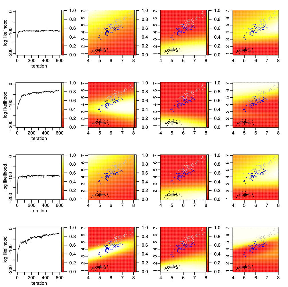
Figure 1: Log-likelihood plots and predictive probability heat maps for the 2-D iris data with a fixed category-stick mapping $\boldsymbol{z}=(1,2,3)$. Blue, black, and gray points are labeled as categories 1, 2, and 3, respectively. For the first row, $K=1$ and $T=1$, second row, $K=1$ and $T=3$, third row, $K=5$ and $T=1$, and fourth row, $K=5$ and $T=3$. The log-likelihood plots are shown in Column 1, and the predictive probability heat maps of categories $1$ (blue), $2$ (black), and $3$ (gray) are shown in Columns 2, 3, and 4, respectively.

The results in Figure 1 show that even an unoptimized category-stick mapping, which is unfavorable to MSR with small $K$ and/or $T$, is enforced, empowering each stick-specific binary regression model with a higher capacity (using larger $K$ and/or $T$) can still allow MSR to achieve excellent separations. It is also simple to show that for the data set in Figure 1, even if one chooses low-capacity stick-specific binary regression models by setting $T=1$, one can still achieve good performance with MSR if the category-stick mapping is set as $\boldsymbol{z}=(2,1,3)$, $\boldsymbol{z}=(3,1,2)$, $\boldsymbol{z}=(2,3,1)$, or $\boldsymbol{z}=(3,2,1)$. That is to say, as long as it is not category 1 (blue points) that is mapped to stick 1, MSR with $T=1$ is able to provide satisfactory performance.

6.2 Influence of Category-Stick Mapping and its Inference

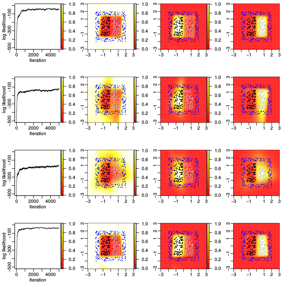
Figure 2: Log-likelihood plots and predictive probability heat maps for the square data with $K=T=10$. The blue, black, and gray points are labeled as categories 1, 2, and 3, respectively. We fix the category-stick mapping as $\boldsymbol{z}=(1,2,3)$ for Row 1, $(2,1,3)$ for Row 2, and $(3,1,2)$ for Row 3, and sample $\boldsymbol{z}$ for Row 4. The log-likelihood plots are shown in Column 1, and the predictive probability heat maps of categories 1 (blue), 2 (black), and 3 (gray) are shown in Columns 2, 3, and 4, respectively.

The Iris data set in Figure 1 provides an instructive example to show not only the importance of increasing the model capacity if a poor category-stick mapping is imposed, but also the importance of optimizing the category-stick mapping if the capacities of these stick-specific binary regression models are limited. To further illustrate the benefits of inferring an appropriate category-stick mapping $\boldsymbol{z}$, we consider the square data set shown in Figure 2. We show that for MSR, even if both $K$ and $T$ are sufficiently large to allow each stick-specific binary regression model to have a high enough capacity, whether an optimal category-stick mapping is selected may still clearly matter for the performance.

As shown in the first three rows of Figure 2, with $K=T=10$, three different $\boldsymbol{z}$’s are considered and $\boldsymbol{z}=(1,2,3)$ (shown in the first row) is found to perform the best. As shown in the fourth row, we sample $\boldsymbol{z}$ using (8) within each MCMC iteration and achieve a result that seems as good as fixing $\boldsymbol{z}=(1,2,3)$. In fact, we find that our inferred mappings switch between $\boldsymbol{z}=(1,2,3)$ and $\boldsymbol{z}=(1,3,2)$ during MCMC iterations, indicating that the Markov chain is mixing well. These results suggest the importance of both learning the mapping $\boldsymbol{z}$ from the data and allowing the stick-specific binary classifiers to have enough capacities to model nonlinear classification decision boundaries.

When sampling $\boldsymbol{z}=(z_{1},\ldots,z_{S})$ that the $S$ categories are mapped to, although $S!$ permutations of $(1,\ldots,S)$ can become enormous as $S$ increases, the effective search space could be much smaller if many different mappings imply similar likelihoods and if these extremely poor mappings can be easily avoided. Rather than searching for the best mapping, the proposed MH step, proposing two indices $z_{j}$ and $z_{j^{\prime}}$ to switch in each iteration, is a simple but effective strategy to escape from the mappings that lead to poor fits. Note that the probability of a $z_{j}$ not being proposed to switch after $t$ MCMC iterations is $[(S-2)/S]^{t}$. Even if $S$ is as large as 100, this probability is less than $10^{-8}$ at $t=1000$. Also note the iteration at which $z_{j}$ is proposed to switch at the first time follows a geometric distribution, with success probability $2/S$. Thus $S/2$ is the expected number of iterations for a $z_{j}$ to be proposed to switch once.

To demonstrate the efficiency of our permutation scheme, we construct square101, a synthetic two-dimensional data set consisting of 101 categories. We generate 8000 data points that are uniformly at random distributed within the $12\times 12$ spatial region occupied by all 101 categories. The decision boundaries of different classes are displayed in Figure 3(a), where the data points placed within the outside square frame, whose outer and inner dimensions are $12$ and $10$, respectively, are assigned to category 1, and these placed within the $s$th unit square, where $s\in\{2,\ldots,101\}$, inside the square frame are assigned to category $s$. Although it is almost impossible to search for the best category-stick mapping $\boldsymbol{z}$ giving rise to the highest likelihood from all $101!\approx 10^{160}$ possible mappings, we show our permutation scheme is very effective in escaping from poor mappings, leading to a performance that is comparable to the best of those obtained with pre-fixed suboptimal mappings. More specifically, applying the analysis in Section 4.2 to Figure 3(a), we expect an aSB-MSR to perform well under a fixed suboptimal category-stick mapping $\boldsymbol{z}$, where $z_{1}=1$, which means the outside square frame is mapped to stick 1, and the squares closer to the inner boundary of the square frame are mapped to the sticks broken at earlier stages; the mapping $\boldsymbol{z}=(1,2,\cdots,101)$ is such an example. In other words, we first separate the frame from all the other squares, and then sequentially separate the squares from the remainders; the closer a square is from the frame, the earlier it is separated. The total number of suboptimal mappings $\boldsymbol{z}$’s constructed in this manner is as large as $36!\times 28!\times 20!\times 12!\times 4!\approx 10^{99.5}$.

First, we uniformly at random generate 3600 different suboptimal mappings $\boldsymbol{z}$’s under this construction, run aSB-MSR with $K=T=4$, and plot the histogram of the 3600 log-likelihoods in Figure 3(b). Second, we start from 3600 randomly initialized $\boldsymbol{z}$, run paSB-MSR with $K=T=4$, and also plot the histogram of the 3600 log-likelihoods in Figure 3(b). For each run, we choose 20,000 MCMC iterations and collect the last 1000 MCMC samples. Each log-likelihood is averaged over those of the corresponding model’s collected MCMC samples. As in Figure 3(b), the log-likelihood from a paSB-MSR is in general clearly larger than that of an aSB-MSR with a fixed suboptimal $\boldsymbol{z}$, and there is little overlap between their corresponding histograms. Further examining the 3600 $\boldsymbol{z}$’s inferred by paSB at its last MCMC iteration shows that 3482 of them have $z_{1}=1$ and all of them have $z_{1}\leq 5$. Suppose $z_{1}\notin\{1,2,3,4,5\}$ at the current iteration, which means category 1 is mapped to none of the first five sticks, then the probability of not only selecting stick $z_{1}$, but also switching it with one of the first five sticks in the MH proposal is $\frac{1}{101}\times\frac{5}{100}$. Thus the probability that category 1 has never been proposed to mapped to one of the first five sticks after $t$ iterations is $\left[1-{5}/({101\times 100})\right]^{t}$, which becomes as small as $0.005\%$ at $t=20,000$, demonstrating the effectiveness of our permutation scheme in dealing with a large number of categories. Note we have also tried 3600 aSB-MSR, each of which is provided with a randomly initialized $\boldsymbol{z}$. The log-likelihoods, however, are all far below $-4000$ and hence not included for comparison. This phenomenon is not surprising, as the probability for a randomly initialized $\boldsymbol{z}$ to be suboptimal is as tiny as $36!\times 28!\times 20!\times 12!\times 4!/101!\approx 10^{-60.5}$.

(a)

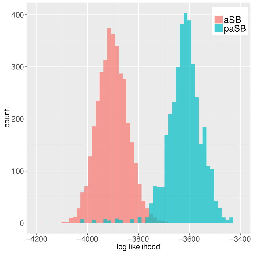
(b)

Figure 3: (a) Illustration of the square101 data and (b) log-likelihood histograms, by aSB-MSR with 3600 random suboptimal category-stick mappings and by paSB-MSR with 3600 randomly initialized category-stick mappings.

Figure 4 empirically demonstrates the effectiveness of permuting $\boldsymbol{z}$ on the satimage data set, using MSRs with $K=5$, $T=3$, and $\boldsymbol{z}$ fixed at each of the $6!=720$ possible one-to-one category-stick mappings. Panels (a) and (b) show the log-likelihood histograms for MSRs constructed under augmented SB (aSB) and augmented reversed SB (arSB), respectively. Both histograms are clearly left skewed, indicating under both aSB and arSB, only a small proportion of the 720 different category-stick mappings lead to very poor fits. The blue vertical lines at $-1203.82$ in (a) and $-1350.21$ in (b) are the log-likelihoods by paSB and parSB, respectively, in both of which the category-stick mapping $\boldsymbol{z}$ is updated by a MH step in each MCMC iteration. Only 20 (97) out of 720 aSB-MSRs (arSB-MSRs) have a higher likelihood than paSB-MSR (parSB-MSR).

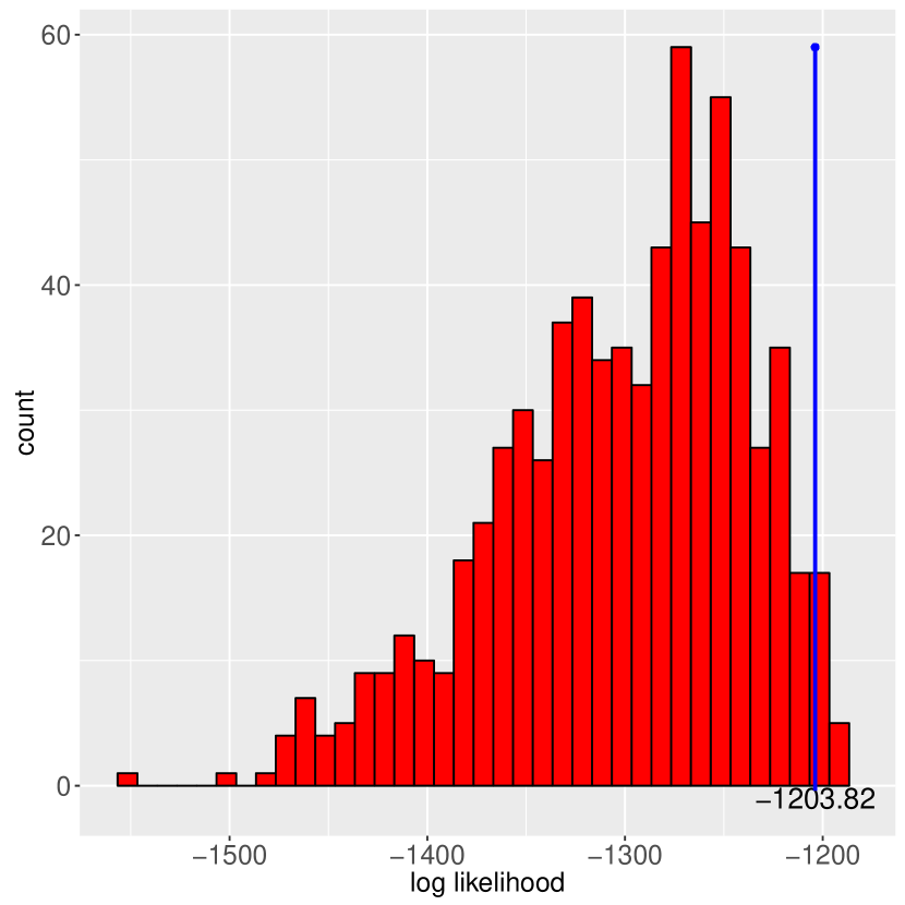
(a) aSB

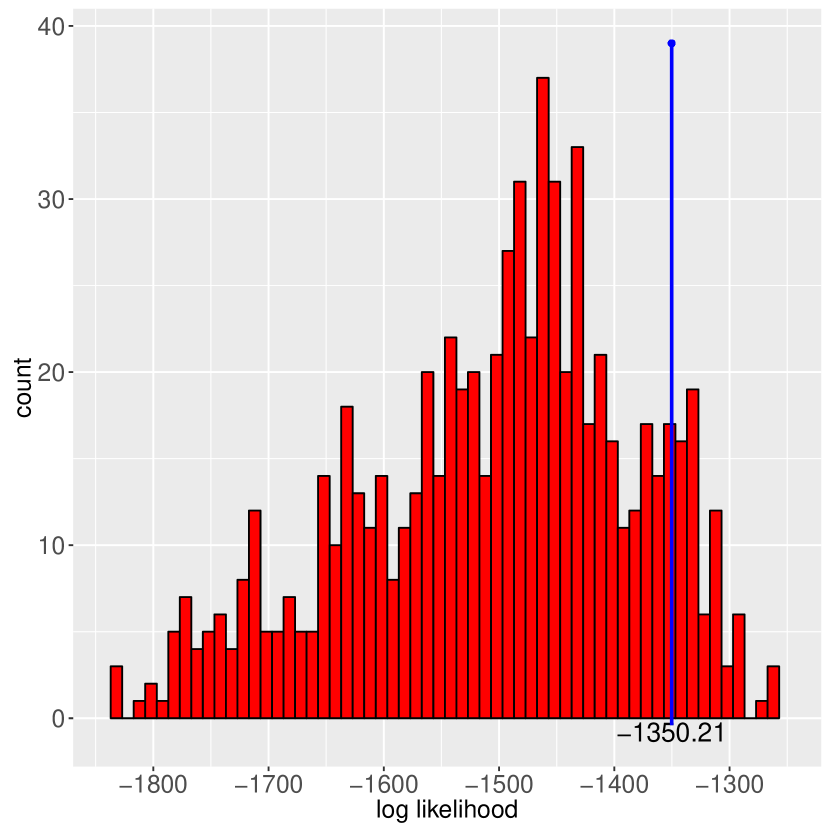
(b) arSB

Figure 4: Log-likelihood histograms for MSRs using all 720 possible category-stick mappings, constructed under (a) augmented stick breaking (aSB) and (b) augmented and reversed stick breaking (arSB). The blue lines in (a) and (b) correspond to the log-likelihoods of paSB-MSR and parSB-MSR, respectively.

Since in the stick-breaking construction, the binary classifier that separates a category mapped to a smaller-indexed stick from the others utilizes fewer constraints, the classification can be poor if the complexity of the decision boundary goes beyond the nonlinear modeling capacity of the binary classifier. However, even with a low-capacity binary classifier, the performance could be significantly improved if that difficult-to-separate category is mapped to a larger-indexed stick, for which there are fewer categories left to be separated in its “one-vs-remaining” binary classification problem. Examining the $\boldsymbol{z}$’s associated with the 100 lowest log-likelihoods in Figure 4, we find there are 51 mappings belonging to the set $\{\boldsymbol{z}:z_{5}=1$ or $z_{6}=1\}$ in aSB, and 77 belonging to $\{\boldsymbol{z}:z_{3}=1$ or $z_{6}=1\}$ in arSB. It suggests that separating Categories 5 or 6 (Categories 3 or 6) from all the other categories might be beyond the capacity of a binary softplus regression with $K=5$ and $T=3$ under the aSB (arSB) construction. But if breaking the sticks associated with these categories at late stages, we only need to separate them from fewer remaining categories, which could be much easier. We have further examined the other 620 arrangements, and found no evident patterns. These observations suggest that the effective search space of the mapping $\boldsymbol{z}$ is considerably smaller than $S!$, and the proposed MH step is effective in escaping from poor category-stick mappings.

In paSB-MSVM, we use a Gaussian radial basis function kernel, whose kernel width is cross validated from a set of predefined candidates. We find its performance to be sensitive to the setting of the kernel width, which is a common issue for SVMs (Cherkassky and Ma, 2004; Soares et al., 2004; Chang et al., 2005). If an appropriate kernel width could be identified through cross validation, we find that learning the mapping $\boldsymbol{z}$ becomes less important for paSB-MSVM to perform well. However, we find that if the kernel width is not well selected, which can happen if all candidate kernel widths are far from the optimal value, the binary classifier for each category may not have enough capacity for nonlinear classification and the learning of the category-stick mapping $\boldsymbol{z}$ could then become important.

6.3 Turning Off Unneeded Model Capacities

Figure 5: Inferred expert weights $r_{k}$ in descending order for each category of the square data with $K=T=10$.

While one can adjust both $K$ and $T$ to control the capacity of binary softplus regression, for MSR, the total number of experts $K$ is a truncation level that can be set as large as permitted by the computation budget. This is because the truncated gamma process used by each stick-specific binary softplus regression shrinks the weights of unnecessary experts towards zeros. Figure 5 shows in decreasing order the inferred weights of the experts belonging to each of the 3 categories of the square data set. These weights are inferred by MSR with $K=T=10$ and the learning of $\boldsymbol{z}$, as in the fourth row of Figure 2. It is clear from Figure 5 that only a small number of experts are inferred with non-negligible weights in the posterior, and the number of active experts and their weights indicate the complexity of the corresponding classification decision boundaries shown in the fourth row of Figure 2. We note that while $T$ is a parameter to be set by the user, we find increasing it increases model capacity, without observing clear signs of overfitting for all the data considered here.

6.4 MSR with Data Transformation

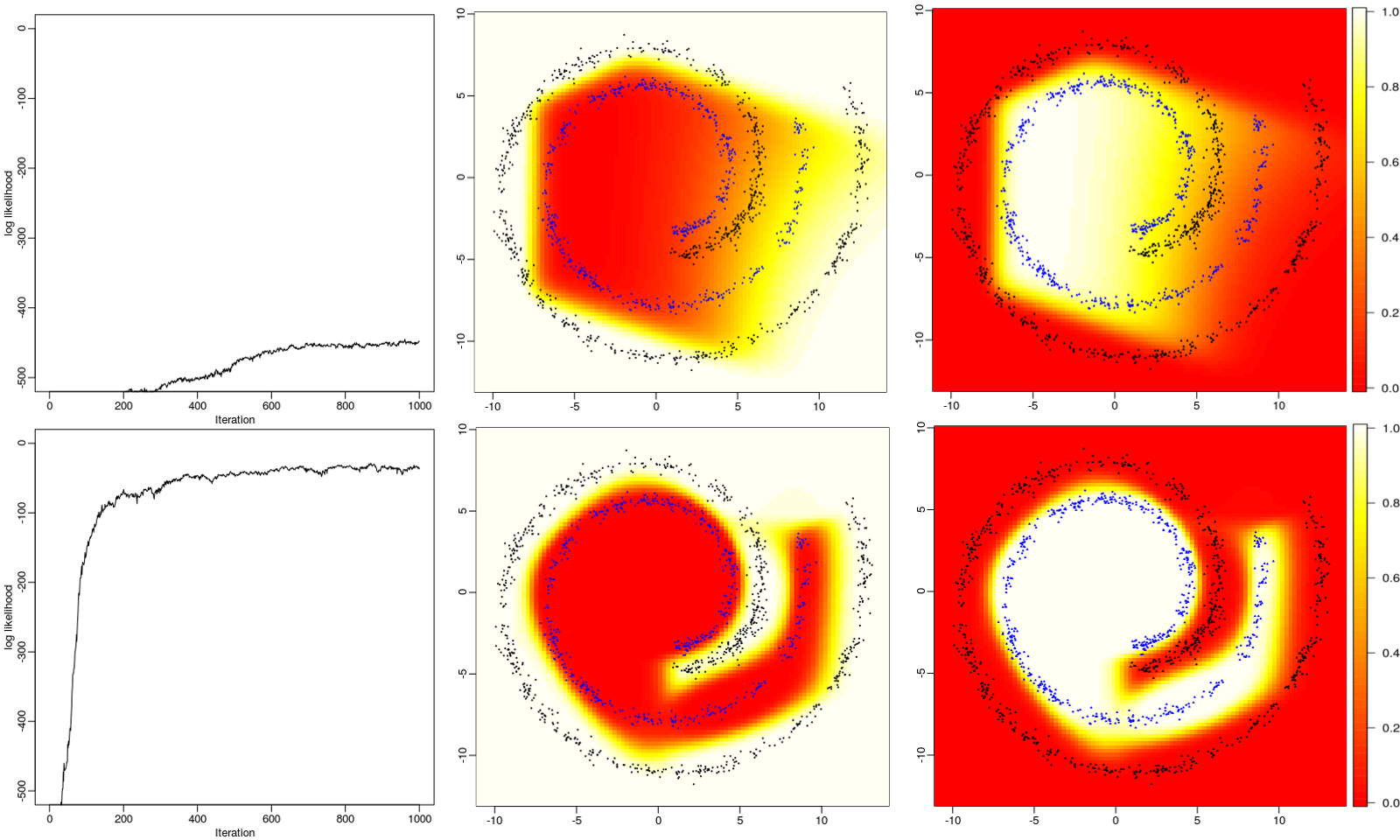
Figure 6: First row: classification of a 2-D swiss roll data by paSB-MSR with $K=5$, $T=3$, using the original covariates. Second row: paSB-MSR with $K=5$, $T=1$ trained on the covariates transformed via the paSB-MSR used in the first row. In each row, the left column plot the log-likelihood against MCMC iteration, and the middle and right columns show the predictive probability heatmaps for Category 1 (black points) and Category 2 (blue points), respectively.

Kernel SVMs transform the data to make different categories more linearly separable in the transformed covariate space. While kernel SVMs may provide high nonlinear modeling capacity, its performance could be sensitive to the kernel width, which often needs to be cross validated, and its number of support vectors often increases linearly in the size of the training set. By contrast, MSRs rely on the interactions of linear hyperplanes to construct nonlinear decision boundaries, as discussed in Section 4.2, and hence may have insufficient capacity for highly complex nonlinearity. However, we may simply stack another MSR on a previously trained MSR to quickly enhance its nonlinear modeling capacity. In particular, we may first run a MSR to obtain a finite set of hyperplanes denoted by $\tilde{{\boldsymbol{\beta}}}_{jk}^{(t+1)}$. We may then augment the original covariate vector $\boldsymbol{x}_{i}$ as

$$\tilde{\boldsymbol{x}}_{i}:=\left[\boldsymbol{x}_{i}^{\prime},\log\big{(}1+e^{\boldsymbol{x}_{i}^{\prime}\tilde{{\boldsymbol{\beta}}}_{11}^{(2)}}\big{)},\cdots,\log\big{(}1+e^{\boldsymbol{x}_{i}^{\prime}\tilde{{\boldsymbol{\beta}}}_{jk}^{(t+1)}}\big{)},\cdots,\log\big{(}1+e^{\boldsymbol{x}_{i}^{\prime}\tilde{{\boldsymbol{\beta}}}_{SK}^{(T+1)}}\big{)}\right]^{\prime}$$ (14)

and run another MSR with the transformed covariates $\tilde{\boldsymbol{x}}_{i}$.

For illustration, we show the efficacy of this data-transformation strategy on a 2-D swiss roll data in Figure 6. The first row shows the results of MSR with $K=5$ and $T=3$, using the original covariates $\boldsymbol{x}_{i}$, while the second row shows MSR with $K=5$ and $T=1$, using the transformed covariates $\tilde{\boldsymbol{x}}_{i}$ defined by (14), where the regression coefficient vectors $\tilde{{\boldsymbol{\beta}}}_{jk}^{(t+1)}$ are learned using the MSR illustrated in the first row. It is evident that the classification is greatly improved in terms of both training log-likelihood and out-of-sample predictions.

6.5 Results on Benchmark Data Sets

To further evaluate the performance of the proposed paSB multinomial regression models, we consider paSB multinomial logistic regression (paSB-MLR), paSB multinomial robit with $\kappa=6$ degrees of freedom (paSB-robit), paSB multinomial support vector machine (paSB-MSVM), and MSRs. We compare their performance with those of $L_{2}$ regularized multinomial logistic regression ($L_{2}$-MLR), support vector machine (SVM), and adaptive multi-hyperplane machine (AMM), and consider the following benchmark multi-class classification data sets: iris, wine, glass, vehicle, waveform, segment, dna, and satimage. We also include the synthetic square data shown in Figure 2 for comparison. For SVM we use the LIBSVM package, which trains $S(S-1)/2$ one-vs-one binary classifiers and makes prediction using majority voting (Chang and Lin, 2011). We run LIBSVM in R with package e1071 (Meyer et al., 2015). We consider MSRs with $(K,T)$ as $(1,1)$, $(1,3)$, $(5,1)$, and $(5,3)$, respectively. We also consider MSR with data transformation (DT-MSR), in which we first train a MSR with $K=5$ and $T=3$ to transform the covariates and then stack another MSR with $K=5$ and $T=1$. We provide detailed descriptions on the data and experimental settings in the Appendix.

With the number of categories in parentheses right after the data set names, we summarize in Table 1 the classification error rates by various models, where those of MSRs are calculated by averaging over paSB and parSB. Table 1 shows that an MSR with $K$ or $T$ sufficiently large generally outperforms paSB-MLR, paSB-robit, $L_{2}$-MLR, and AMM, and using another MSR on the transformed covariates can in general further reduce the error rate. This is especially evident when there are nonlinearly separable categories, as indicated by a clearly higher error rate of $L_{2}$-MLR in contrast to that of SVM. One may notice that paSB-robit, paSB-MLR, and MSR with $K=T=1$ are similar to $L_{2}$-MLR in terms of performance, suggesting the effectiveness of the proposed permutation scheme, which helps mitigate the potential adverse effects of having asymmetric class labels. One may also note that paSB-robit outperforms paSB-MLR on glass, vehicle, waveform, dna, and satimage, indicating there are benefits in using a robust classifier on these data sets. Comparable error rates of paSB-MSVM to SVM and better performance of MSRs on most data sets demonstrate the success of the paSB framework in transforming a binary classifier with cross entropy loss into a Bayesian multinomial one.

Data (S) paSB-MLR paSB-robit paSB-MSVM $K=1$ $T=1$ $K=1$ $T=3$ $K=5$ $T=1$ $K=5$ $T=3$ DT-MSR $L_{2}$-MLR SVM AMM square(3) 59.52 67.46 0 57.14 15.08 0 0 0 62.29 4.76 16.67 iris(3) 4.00 5.33 3.33 4.67 4.00 4.00 4.00 3.33 3.33 4.00 4.67 wine(3) 4.44 5.00 2.78 2.78 2.22 2.78 2.22 2.78 3.89 2.78 3.89 glass(6) 35.35 34.88 29.30 33.49 26.05 31.16 32.09 26.37 33.02 28.84 37.67 vehicle(4) 23.23 21.25 17.32 22.44 17.32 17.72 15.75 14.96 22.83 18.50 21.89 waveform(4) 17.87 16.42 15.76 19.84 16.62 15.67 15.04 15.56 15.60 15.22 18.54 segment(7) 7.36 8.03 7.98 6.20 6.49 6.45 5.63 7.65 8.56 6.20 12.47 dna(3) 5.06 4.05 5.31 4.13 4.47 4.55 4.22 3.88 5.98 4.97 5.43 satimage(6) 20.65 17.25 8.90 16.65 14.45 12.85 12.00 9.85 17.80 8.50 15.31

Table 1: Comparison of the classification error rates (%) of paSB-MLR, paSB-robit, paSB-MSVM, MSRs with various $K$ and $T$ (columns 5 to 8), MSR with data transformation (DT-MSR), $L_{2}$-MLR, SVM, and AMM.

To further check whether a paSB model is attractive when fast out-of-sample prediction is desired, we consider using only the MCMC sample that has the highest training likelihood among the collected ones for all paSB models, and summarize in Table 4 of the Appendix the classification error rates of various models, with the number of inferred support vectors or active hyperplanes included in parenthesis. Following the definition of active experts in Zhou (2016), we define for MSRs the number of active hyperplanes as $T\sum_{s}^{S}\widetilde{K}_{s}$ where $\widetilde{K}_{s}$ is the number of active experts for class $s$. The number of active hyperplanes determines the computational complexity for out-of-sample prediction with a single MCMC sample, which is $O(T\sum_{s}^{S}\widetilde{K}_{s})$. Since the error rates of MSRs in Table 4 are calculated by averaging over both paSB and parSB, the number of active hyperplanes is $T\sum_{s}^{S}(\widetilde{K}_{s}^{(paSB)}+\widetilde{K}_{s}^{(parSB)})$.

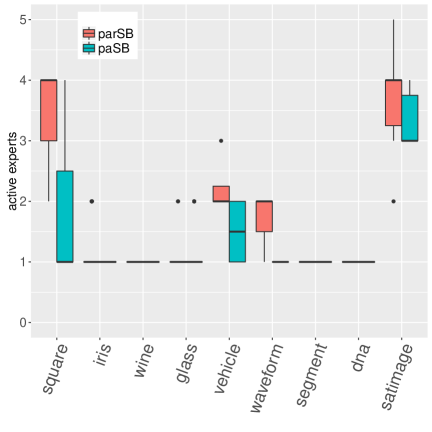
Figure 8: Boxplots of the number of active experts inferred by paSB/parSB MSRs with $K=5$ and $T=3$.

Shown in Figure 8 in the Appendix are boxplots of the number of each category’s active experts for MSR with $K=5$ and $T=3$. Except for several categories of satimage that require all $K=5$ experts for parSB-MSR, $K=5$ is large enough to provide the needed model capacity under all the other scenarios. As shown in Table 4, MSRs with sufficiently large $K$ and/or $T$ are comparable to both SVM and paSB-MSVM in terms of the error rates, while clearly outperforming them in terms of the number of (active) hyperplanes/support vectors and hence computational complexity for out-of-sample predictions. While MSR with $K=T=1$, paSB-MLR, and paSB-robit generally perform worse than SVM in terms of the error rates, they use much fewer hyperplanes and hence have significantly lower computation for out-of-sample predictions. In summary, MSR whose upper-bound for the number of active expects $K$ and number of layers for each expert $T$ can both be adjusted to control its capacity of modeling nonlinearity, can achieve a good compromise between the accuracy and computational complexity for out-of-sample prediction of multinomial class probabilities, and can be further improved by training an additional MSR on the transformed covariates.

$10\%$ quantile median $90\%$ quantile training testing training testing training testing Bayes MLR paSB-MLR Bayes MLR paSB-MLR Bayes MLR paSB-MLR Bayes MLR paSB-MLR Bayes MLR paSB-MLR Bayes MLR paSB-MLR square 411.46 194.54 421.62 256.48 913.17 948.53 858.46 952.33 924.48 973.60 927.93 976.33 iris 82.30 90.33 73.75 84.40 149.47 218.21 156.25 174.16 331.71 854.45 341.39 793.00 wine 194.41 314.41 58.41 56.30 467.73 859.67 506.66 643.90 926.55 991.46 958.12 994.77 glass 70.18 162.69 67.81 138.90 137.18 335.14 122.27 329.21 359.75 686.43 347.40 615.02 vehicle 77.71 103.30 74.05 101.64 133.66 230.83 127.22 230.48 426.44 460.07 414.48 453.87 waveform 123.77 120.01 120.99 113.94 199.00 203.38 191.77 209.61 310.84 499.05 291.96 478.59 segment 114.91 104.77 95.63 91.31 281.11 294.17 270.63 355.46 742.63 844.11 752.74 814.62 dna 217.99 238.48 63.66 67.26 481.65 736.58 505.59 772.32 911.68 986.60 927.30 991.63 satimage 53.51 66.19 54.04 66.33 82.50 90.50 81.87 90.11 160.84 168.85 156.83 157.31

Table 2: Comparison of the ESS of the conditional class probability between Bayes MLR and paSB-MLR.

We further measure how well the Gibbs sampler is mixing using effective sample size (ESS) for both paSB-MLR and Bayesian multinomial logistic regression (Bayes MLR) of Polson et al. (2013). For both algorithms we let ${\boldsymbol{\beta}}_{j}\sim\mathcal{N}\left(0,\mbox{diag}(\alpha_{j0}^{-1},\ldots,\alpha_{jV}^{-1})\right)$, where $\alpha_{jv}\sim\mbox{Gamma}(0.001,1/0.001).$ The ESS (Holmes and Held, 2006) of a parameter or a function of parameters is defined as $\mbox{ESS}=L/\left[1+2\sum_{h=1}^{\infty}\rho(h)\right],$ where $L$ is the number of post-burn-in samples, $\rho(h)$ is the $h$th autocorrelation of the parameter or the function of parameters. It describes how quickly an MCMC algorithm generates independent samples. Since the Gibbs sampler of Bayes MLR samples one ${\boldsymbol{\beta}}_{j}$ conditioning on all ${\boldsymbol{\beta}}_{j^{\prime}}$ for $j^{\prime}\neq j$, which may lead to strong dependencies between different categories and hence slow down the mixing of the Markov chain. By contrast, the ${\boldsymbol{\beta}}_{j}$’s are conditionally independent given the augmented variables $b_{ij}$’s in paSB-MLR, which may lead to faster mixing. For both Bayes MLR and paSB-MLR, we consider five independent random trials, in each of which we randomly initialize the model parameters, run 10,000 Gibbs sampling iterations, and collect the last 1,000 MCMC samples of ${\boldsymbol{\beta}}_{j}$. We use the mcmcse package (Flegal et al., 2016) to estimate the ESS of each $p_{ij}$ in a random trial using the 1,000 collected MCMC samples. For the training set, we calculate the 10% quantile, median, and 90% quantile of the ESSs of all $p_{ij}$ for each random trial, and then report their averages over the five random trials in Table 2. For the testing set, we follow the same steps and report the results in Table 2. While paSB-MLR underperforms Bayes MLR on some of the data sets for the 10% ESS quantile, they consistently outperform Bayes MLR on all data sets for both the ESS median and $90\%$ ESS quantile, for both training and testing.

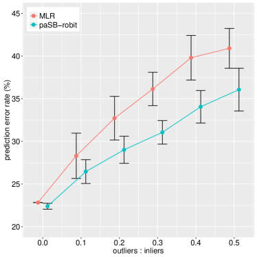
Figure 7: Prediction error rates (%, mean $\pm$ standard deviation) for different ratios of outliers to inliers.

6.6 Robustness of paSB-Robit Regression

We use the contaminated vehicle data to demonstrate the robustness of paSB-robit. As discussed by Liu (2004), the heavy-tailed conditional class probability function of robit regression can robustify the decision boundary when there exist outliers. We use the vehicle training set as inliers, synthesize outliers that are far from inliers, combine both as the new training set, and keep the testing set unchanged. We generate different numbers of outliers so that the ratio of outliers to inliers varies from $0$, $0.1$, $0.2$, $0.3$, to $0.5$, at each of which we randomly simulate 10 different sets of outlier covariates. We provide the details on how we generate outliers in the Appendix.

We compare $L_{2}$-MLR and paSB-robit with $\kappa=1$ degree of freedom on the contaminated vehicle data. Figure 7 shows the prediction error rate (mean $\pm$ standard deviation) of the testing set for different outlier-inlier ratios. When there are no outliers, both approaches delivers comparable performances. As the ratio increases, paSB-robit with $\kappa=1$ more and more clearly outperforms $L_{2}$-MLR, which justifies the robustness of paSB-robit.

7 Conclusions

To transform a cross-entropy-loss binary classifier into a Bayesian multinomial regression model and derive efficient Bayesian inference, we develop a permuted and augmented stick-breaking construction. With permutation, we one-to-one map the categories to sticks to escape from poor category-stick mappings that impose restrictive geometric constraints on the decision boundaries, and with augmentation, we link a category outcome to conditionally independent stick-specific covariate-dependent Bernoulli random variables. We illustrate this general framework by extending binary softplus regression, robit regression, and support vector machine into multinomial ones. Experiment results validate our contributions and show that the proposed multinomial softplus regressions achieve a good compromise between interpretability, complexity, and predictability.

Acknowledgments

The authors would like to thank the editor and two anonymous referees for their insightful and constructive comments and suggestions, and Texas Advanced Computing Center for computational support.

A Additional Lemma and Proofs

Proof [Proof of Theorem 1] The conditional probability of $y_{i}$ given $\{z_{s},\pi_{is}\}_{1,S}$ can be expressed as

$$\footnotesize\textstyle P(y_{i}=s\,|\,\{z_{s},\pi_{is}\}_{1,S}) =\textstyle\sum_{b_{ij}:j>z_{s}}\textstyle\left[P(b_{iz_{s}}=1)\right]^{\mathbf{1}(z_{s}\neq S)}\left[\prod_{j<z_{s}}P(b_{ij}=0)\right]\left[\prod_{j>z_{s}}P(b_{ij})\right]$$

$$=\textstyle\left[P(b_{iz_{s}}=1)\right]^{\mathbf{1}(z_{s}\neq S)}\left[\prod_{j<z_{s}}P(b_{ij}=0)\right]\sum_{b_{ij}:j>z_{s}}\left[\prod_{j>z_{s}}P(b_{ij})\right],$$

which becomes the same as (4) by applying (5) and $\sum_{b_{ij}:j>z_{s}}\!\big{[}\prod_{j>z_{s}}\!P(b_{ij})\big{]}\!=\!1$.  

Proof [Proof of Lemma 3] Under the paSB construction, the probability ratio of categories (choices) $s$ and $s+d$ is a function of the stick success probabilities $\pi_{z_{s}},\pi_{z_{(s+1)}},\cdots,\pi_{z_{(s+d)}}$. More specifically,

$$\frac{p_{i(s+d)}(\boldsymbol{z})}{p_{is}(\boldsymbol{z})}=\frac{\pi_{iz_{(s+d)}}^{\mathbf{1}(z_{(s+d)}\neq S)}\left[\prod_{z_{s}\leq j<z_{(s+d)}}(1-\pi_{ij})\right]^{\delta(z_{s}\leq z_{(s+d)})}}{\pi_{iz_{s}}^{\mathbf{1}(z_{s}\neq S)}\left[\prod_{z_{(s+d)}\leq j<z_{s}}(1-\pi_{ij})\right]^{\delta(z_{s}>z_{(s+d)})}}.\vspace{0mm}$$

 

Proof [Proof of Lemma 4] Since $p_{is}(\boldsymbol{z})=\left[1-\big{(}{1+e^{\boldsymbol{x}_{i}^{\prime}{\boldsymbol{\beta}}_{s}}}\big{)}^{-r_{s}}\right]^{\mathbf{1}(s\neq S)}\prod_{j<s}\big{(}{1+e^{\boldsymbol{x}_{i}^{\prime}{\boldsymbol{\beta}}_{j}}}\big{)}^{-r_{j}}$ when $K=T=1$ and $\boldsymbol{z}=(1,\ldots,S)$, the set of solutions to $p_{is}>p_{0}$ are bounded by the set of solutions to $\big{(}{1+e^{\boldsymbol{x}_{i}^{\prime}{\boldsymbol{\beta}}_{j}}}\big{)}^{-r_{s}}>p_{0},~{}j\in\{1,\ldots,s-1\},$ and $1-\big{(}{1+e^{\boldsymbol{x}_{i}^{\prime}{\boldsymbol{\beta}}_{s}}}\big{)}^{-r_{s}}>p_{0},$ and hence bounded by the convex polytope defined by the set of solutions to the $s$ inequalities as

$$\boldsymbol{x}_{i}^{\prime}[(-1)^{\mathbf{1}(j=s)}{\boldsymbol{\beta}}_{j}]<(-1)^{\mathbf{1}(j=s)}\ln\left\{\left[p_{0}^{\mathbf{1}(j\neq s)}(1-p_{0})^{\mathbf{1}(j=s)}\right]^{-\frac{1}{r_{j}}}-1\right\},~{}~{}j\in\{1,\ldots,s\}.\vspace{0mm}$$

 

Lemma 5

Without loss of generality, let us assume that the category-stick mapping is fixed at $\boldsymbol{z}=(1,2,\cdots,S)$. The paSB multinomial logistic model that assigns choice $s\in\{1,\ldots,S\}$ for individual $i$ with probability $p_{is}=(\pi_{is})^{\mathbf{1}(s\neq S)}\prod_{j<s}(1-\pi_{ij})$, where $\pi_{is}=1/(1+e^{-W_{is}})$, can be considered as a sequential random utility maximization model. This model selects choice $s$ once $U_{is}>\sum_{j\geq s}U_{ij}$ is observed for $s=1,\ldots,S$, where $U_{is}$ are defined as

$$U_{i1} =U_{i2}+\cdots+U_{iS}+W_{i1}+\varepsilon_{i1},$$

$$\cdots$$

$$U_{is} =\sum_{j>s}U_{ij}+W_{is}+\varepsilon_{is},$$

$$\cdots$$

$$U_{i(S-1)} =W_{i(S-1)}+\varepsilon_{i(S-1)},$$

$$U_{iS} =0,$$

and $\varepsilon_{is}\overset{i.i.d.}{\sim}\emph{\mbox{Logistic}}(0,1)$ are independent, and identically distributed (i.i.d.) random variables following the standard logistic distribution.

Proof [Proof of Lemma 5] Note that $P(\varepsilon<x)=1/(1+e^{-x})$ if $\varepsilon\sim\mbox{Logistic}(0,1)$. First consider the choice of individual $i$ be $y_{i}=1$, which would happen with probability

$$P(y_{i}=1)=P\left(U_{i1}>\sum\nolimits_{j\geq 1}U_{ij}\right)=P(\varepsilon_{i1}>-W_{i1})=1/(1+e^{-W_{i1}})=\pi_{i1}=p_{i1}.$$

Then for $s=2,\cdots,S-1$,

$$P(y_{i}=s) =P(y_{i}=s\,|\,y_{i}>s-1)P(y_{i}>s-1)$$

$$=P\left(U_{is}>\sum\nolimits_{j>s}U_{ij}\right)\prod\nolimits_{j\leq s-1}P\left(U_{ij}<\sum\nolimits_{j^{\prime}>j}U_{ij^{\prime}}\right)$$

$$=P(\varepsilon_{is}>-W_{is})\prod\nolimits_{j\leq s-1}P(\varepsilon_{ij}<-W_{ij})$$

$$=\pi_{is}\prod\nolimits_{j\leq s-1}(1-\pi_{ij})$$

$$=p_{is}.$$

Finally, $P(y_{i}=S)=1-\sum_{j<S}P(y_{i}=j)=\prod_{j<S}(1-\pi_{ij})=p_{iS}$.  

B Experimental Settings and Additional Results

The table below summarizes the sizes of both training and testing sets, and the number of covariates and categories. The training and testing sets are predefined for vehicle, dna, and satimage. Note that the training and validation sets are combined as training. We divide the other data sets into training and testing as follows. For iris, wine, and glass, five random partitions are taken such that for each partition the training set accounted for 80% of the whole data set while the testing set 20%. The classification error rate is calculated by averaging the error rates of all five random partitions. For square, waveform, and segment, only one random partition is taken, where 70% of the square data set are used as training and the remaining 30% as testing, and 10% of both the waveform and segment datas are used as training and the remaining 90% as testing.

	square	iris	wine	glass	vehicle	waveform	segment	dna	satimage
Train size	294	120	142	171	592	500	231	2000	4435
Test size	126	30	36	43	254	4500	2079	1186	2000
Covariate number	2	4	13	9	18	21	19	180	36
Category number	3	3	3	6	4	3	7	3	6

Table 3: Multi-class classification data sets used in experiments for model comparison.

We compare paSB-MLR, paSB-robit with $\kappa=6$, paSB-MSVM, and MSR with three other models, including $L_{2}$ regularized multinomial logistic regression ($L_{2}$-MLR), support vector machine (SVM), and adaptive multi-hyperplane machine (AMM). For paSB-robit, we run 8,000 iterations and discard the first 5,000 as burn-in (this setting is unchanged for experiments in Section 6.6). For paSB-MSVM, we use the spike-and-slab prior to select the kernel bases and set $0.5$ as the probability of spike at $0$, which is referred to as a uniform prior by Polson and Scott (2011). A Gaussian radial basis function (RBF) kernel is used and the kernel width is selected by 3-fold cross validation from $(2^{-10},2^{-9},\ldots,2^{10})$. We run 1000 MCMC iterations and discard the first 500 as burn-in samples. For MSR, we try both paSB and parSB with $(K,T)$ set as $(1,1)$, $(1,3)$, $(5,1)$, or $(5,3)$. We run 10000 MCMC iterations and discard the first 5000 as burn-in samples. The predictive probability is calculated by averaging the Monte Carlo average predictive probabilities from paSB and parSB MSRs. An observation in the testing set is classified to the category associated with the largest predictive probability.

paSB-MLR paSB-robit paSB-MSVM $K=1$ $T=1$ $K=1$ $T=3$ $K=5$ $T=1$ $K=5$ $T=3$ DT-MSR $L_{2}$-MLR SVM AMM square 53.17(2) 57.94(2) 0(256) 57.14(4) 13.49(12) 1.59(10) 0.79(33) 1.59(40) 62.29(2) 4.76(22) 16.67(7) iris 2(2) 6.67(2) 3.33(97.6) 4.67(4) 4.67(12) 4(5.4) 3.33(12) 4.67(16.2) 3.33(2) 4(35) 4.67(8.6) wine 8.33(2) 4.86(2) 2.14(125.8) 4.45(4) 4.45(12) 6.67(4) 3.34(12) 3.89(16.4) 3.89(2) 2.78(77.2) 3.89(7.8) glass 39.07(5) 34.41(5) 30.23(137.6) 35.35(10) 30.7(30) 33.02(10.4) 35.81(33.2) 32.56(47.8) 33.02(5) 28.84(118) 37.67(23.8) vehicle 25.98(3) 22.44(3) 17.71(592) 23.62(6) 21.65(18) 18.9(12) 16.93(33) 18.11(45) 22.83(3) 18.50(256) 21.89(17) waveform 18.78(2) 16.84(2) 16.56(500) 19.73(4) 17.11(12) 17.07(6) 17.11(18) 16.49(23) 15.60(2) 15.22(212) 18.54(11.6) segment 7.07(6) 9.81(6) 9.86(231) 8.61(12) 8.37(36) 7.31(13) 7.79(36) 8.85(50) 8.56(6) 6.20(93) 12.47(11.4) dna 6.58(2) 4.30(2) 7.25(1701) 5.56(4) 5.73(12) 6.07(7) 5.82(12) 4.72(17) 5.98(2) 4.97(1142) 5.43(18.6) satimage 21.35(5) 16.40(5) 9.5(4315) 15.8(10) 14.7(30) 13.25(34) 11.95(102) 11.55(105) 17.80(5) 8.50(1652) 15.31(16.8)

Table 4: Comparison of classification error rates (%) of paSB-MLR, paSB-robit, paSB-MSVM, MSRs with various $K$ and $T$ (results column 3 to 6), MSR with data transformation (DT-MSR), $L_{2}$-MLR, SVM, and AMM, using the collected MCMC sample with the highest log-likelihood. The number of active hyperplanes/support vectors used for out-of-sample predictions are shown in parenthesis.

For MSRs on benchmark data with data transformation, in the first step, we run paSB-MSR and parSB-MSR with $K=5$ and $T=3$ on the original covariates for 3,000 iterations to learn $\boldsymbol{z}$, $\{r_{jk}\}$, $\{{\boldsymbol{\beta}}_{jk}^{(t)}\}$. We then transform the covariates by Equation (6.4), where ${\boldsymbol{\beta}}_{jk}^{(t)}$ are associated with active experts. In the last step, we use $\boldsymbol{z}$ learned in the first step, and run paSB-MSR and parSB-MSR with $K=5$ and $T=1$ for 10,000 iterations and collect the last 5,000 samples to compute the predictive probabilities.

We use the $L_{2}$-MLR provided in the LIBLINEAR package (Fan et al., 2008) to train a linear classifier, where a bias term is included and the regularization parameter is five-fold cross-validated on the training set from $(2^{-10},2^{-9},\ldots,2^{15})$. We run the LIBLINEAR package in R via R package LiblineaR (Helleputte, 2015). We also classify an observation to the category associated with the largest predictive probability. For SVM, we use the LIBSVM package (Chang and Lin, 2011) and run it in R with R package e1071 (Meyer et al., 2015). A Gaussian RBF kernel is used and three-fold cross validation is adopted to tune both the regularization parameter and kernel width from $(2^{-10},2^{-9},\ldots,2^{10})$ on the training set. For paSB-MSVM, we use three-fold cross validation on the training set to select a kernel width from $(2^{-10},2^{-9},\ldots,2^{10})$. We choose the default LIBSVM settings for all the other parameters. We consider adaptive multi-hyperplane machine (AMM) of Wang et al. (2011b), as implemented in the BudgetSVM (Version 1.1) software package (Djuric et al., 2013). We use the batch version of the algorithm. Important parameters of the AMM include both the regularization parameter $\nu$ and training epochs $E$. As also mentioned by Kantchelian et al. (2014), we do not observe the testing errors of AMM to strictly decrease as $E$ increased. Thus, in addition to cross validating the regularization parameter $\nu$ on the training set from $\{10^{-7},10^{-6},\ldots,10^{-2}\}$, as done in Wang et al. (2011b), for each $\nu$, we try $E\in\{5,10,20,50,100\}$ sequentially until the cross-validation error begins to decrease, $i.e.$, under the same $\nu$, we choose $E=20$ if the cross-validation error of $E=50$ is greater than that of $E=20$. We use the default settings for all the other parameters, and calculate average classification error rates.

We add an outlier to the vehicle data in Section 6.6 as follows. There are 18 covariates, whose values range from $-1$ to $1$, in this data set. To simulate an outlier, since the MLR regression coefficients associated with the 4th, 5th, and 6th covariates all have large absolute values, we first draw three uniform random numbers from $(-3,-2)\cup(2,3)$ and assign them to these three covariates, and then assign each of the 12 remaining covariates a uniform random number from $(-1,1)$. Finally, we draw the category label $y$ uniformly from $\{1,2,3,4\}$.

References

- Albert and Chib [1993] J. H. Albert and S. Chib. Bayesian analysis of binary and polychotomous response data. J. Amer. Statist. Assoc., 88(422):669–679, 1993.
- Blei and Jordan [2006] D. M. Blei and M. I. Jordan. Variational inference for Dirichlet process mixtures. Bayesian Analysis, 1(1):121–143, 2006.
- Boser et al. [1992] B. E. Boser, I. M. Guyon, and V. N. Vapnik. A training algorithm for optimal margin classifiers. In Proceedings of the Fifth Annual Workshop on Computational Learning Theory, pages 144–152. ACM, 1992.
- Chang and Lin [2011] C.-C. Chang and C.-J. Lin. LIBSVM: A library for support vector machines. ACM Transactions on Intelligent Systems and Technology, 2:27:1–27:27, 2011.
- Chang et al. [2005] Q. Chang, Q. Chen, and X Wang. Scaling Gaussian RBF kernel width to improve SVM classification. In 2005 International Conference on Neural Networks and Brain, volume 1, pages 19–22. IEEE, 2005.
- Cherkassky and Ma [2004] V. Cherkassky and Y. Ma. Practical selection of SVM parameters and noise estimation for SVM regression. Neural networks, 17(1):113–126, 2004.
- Chung and Dunson [2009] Y. Chung and D. B. Dunson. Nonparametric Bayes conditional distribution modeling with variable selection. J. Amer. Statist. Assoc., 104:1646–1660, 2009.
- Cortes and Vapnik [1995] C. Cortes and V. Vapnik. Support-vector networks. Machine Learning, 20(3):273–297, 1995.
- Crammer and Singer [2002] K. Crammer and Y. Singer. On the algorithmic implementation of multiclass kernel-based vector machines. J. Mach. Learn. Res., 2:265–292, 2002.
- Cristianini and Shawe-Taylor [2000] N. Cristianini and J. Shawe-Taylor. An Introduction to Support Vector Machines. Cambridge University Press, 2000.
- Djuric et al. [2013] N. Djuric, L. Lan, S. Vucetic, and Z. Wang. Budgetedsvm: A toolbox for scalable SVM approximations. J. Mach. Learn. Res., 14:3813–3817, 2013.
- Dunson and Park [2008] D. B. Dunson and J.-H. Park. Kernel stick-breaking processes. Biometrika, 95(2):307–323, 2008.
- Fan et al. [2008] R.-E. Fan, K.-W. Chang, C.-J. Hsieh, X.-R. Wang, and C.-J. Lin. LIBLINEAR: A library for large linear classification. J. Mach. Learn. Res., pages 1871–1874, 2008.
- Ferguson [1973] T. S. Ferguson. A Bayesian analysis of some nonparametric problems. Ann. Statist., 1(2):209–230, 1973.
- Flegal et al. [2016] James M. Flegal, John Hughes, and Dootika Vats. mcmcse: Monte Carlo Standard Errors for MCMC. Riverside, CA and Minneapolis, MN, 2016. R package version 1.2-1.
- Glorot et al. [2011] X. Glorot, A. Bordes, and Y. Bengio. Deep sparse rectifier neural networks. In AISTATS, pages 315–323, 2011.
- Greene [2003] W. H. Greene. Econometric Analysis. Upper Saddle River, New Jersey: Prentice Hall, 2003.
- Grifin and Steel [2006] J. Grifin and M. Steel. Order-based dependent Dirichlet processes. J. Amer. Statist. Assoc., 2006.
- Grünbaum [2013] B. Grünbaum. Convex Polytopes. Springer New York, 2013.
- Hanemann [1984] W. M. Hanemann. Discrete/continuous models of consumer demand. Econometrica: Journal of the Econometric Society, pages 541–561, 1984.
- Helleputte [2015] T. Helleputte. LiblineaR: Linear Predictive Models Based on the LIBLINEAR C/C++ Library, 2015. R package version 1.94-2.
- Henao et al. [2014] R. Henao, X. Yuan, and L. Carin. Bayesian nonlinear support vector machines and discriminative factor modeling. In NIPS, pages 1754–1762, 2014.
- Hjort et al. [2010] N. L. Hjort, C. Holmes, P. Müller, and S. G. Walker. Bayesian Nonparametrics, volume 28. Cambridge University Press, 2010.
- Holmes and Held [2006] C. C. Holmes and L. Held. Bayesian auxiliary variable models for binary and multinomial regression. Bayesian Analysis, 1(1):145–168, 2006.
- Imai and van Dyk [2005] K. Imai and D. A. van Dyk. A Bayesian analysis of the multinomial probit model using marginal data augmentation. Journal of Econometrics, 124(2):311–334, 2005.
- Ishwaran and James [2001] H. Ishwaran and L. F. James. Gibbs sampling methods for stick-breaking priors. J. Amer. Statist. Assoc., 96(453), 2001.
- Jasra et al. [2005] A. Jasra, C. C. Holmes, and D. A. Stephens. Markov chain Monte Carlo methods and the label switching problem in Bayesian mixture modeling. Statistical Science, pages 50–67, 2005.
- Kantchelian et al. [2014] A. Kantchelian, M. C. Tschantz, L. Huang, P. L. Bartlett, A. D. Joseph, and J. D. Tygar. Large-margin convex polytope machine. In NIPS, pages 3248–3256, 2014.
- Khan et al. [2012] M. E. Khan, S. Mohamed, B. M. Marlin, and K. P. Murphy. A stick-breaking likelihood for categorical data analysis with latent Gaussian models. In AISTATS, pages 610–618, 2012.
- Krizhevsky et al. [2012] A. Krizhevsky, I. Sutskever, and G. E. Hinton. Imagenet classification with deep convolutional neural networks. In NIPS, pages 1097–1105, 2012.
- Kurihara et al. [2007] K. Kurihara, M. Welling, and Y. W. Teh. Collapsed variational Dirichlet process mixture models. In IJCAI, volume 7, pages 2796–2801, 2007.
- LeCun et al. [2015] Y. LeCun, Y. Bengio, and G. Hinton. Deep learning. Nature, 521(7553):436–444, 2015.
- Lee et al. [2004] Y. Lee, Y. Lin, and G. Wahba. Multicategory support vector machines: Theory and application to the classification of microarray data and satellite radiance data. J. Amer. Statist. Assoc., 99(465):67–81, 2004.
- Linderman et al. [2015] S. Linderman, M. Johnson, and R. P. Adams. Dependent multinomial models made easy: Stick-breaking with the Pólya-Gamma augmentation. In NIPS, pages 3438–3446, 2015.
- Liu [2004] Chuanhai Liu. Robit regression: a simple robust alternative to logistic and probit regression. Applied Bayesian Modeling and Casual Inference from Incomplete-Data Perspectives, pages 227–238, 2004.
- Liu and Yuan [2011] Y. Liu and M. Yuan. Reinforced multicategory support vector machines. Journal of Computational and Graphical Statistics, 20(4):901–919, 2011.
- Mallick et al. [2005] B. K. Mallick, D. Ghosh, and M. Ghosh. Bayesian classification of tumours by using gene expression data. J. R. Stat. Soc: Series B, 67(2):219–234, 2005.
- McCullagh and Nelder [1989] P. McCullagh and J. A. Nelder. Generalized linear models, volume 37. CRC press, 1989.
- McCulloch and Rossi [1994] R. McCulloch and P. E Rossi. An exact likelihood analysis of the multinomial probit model. Journal of Econometrics, 64(1):207–240, 1994.
- McCulloch et al. [2000] R. E. McCulloch, N. G. Polson, and P. E. Rossi. A Bayesian analysis of the multinomial probit model with fully identified parameters. Journal of Econometrics, 99(1):173–193, 2000.
- McFadden [1973] D. McFadden. Conditional logit analysis of qualitative choice behavior. Frontiers in Econometrics, pages 105–142, 1973.
- Meyer et al. [2015] D. Meyer, E. Dimitriadou, K. Hornik, A. Weingessel, and F. Leisch. e1071: Misc Functions of the Department of Statistics, Probability Theory Group (Formerly: E1071), TU Wien, 2015. URL https://CRAN.R-project.org/package=e1071. R package version 1.6-7.
- Murphy [2012] K. P. Murphy. Machine Learning: A Probabilistic Perspective. MIT press, 2012.
- Nair and Hinton [2010] V. Nair and G. E. Hinton. Rectified linear units improve restricted Boltzmann machines. In ICML, pages 807–814, 2010.
- Pearl [2014] J. Pearl. Probabilistic Reasoning in Intelligent Systems: Networks of Plausible Inference. Morgan Kaufmann, 2014.
- Pitman [1996] J. Pitman. Some developments of the Blackwell-Macqueen urn scheme. Statistics, Probability, and Game Theory: Papers in Honor of David Blackwell, 30:245–267, 1996.
- Polson and Scott [2011] N. G. Polson and S. L. Scott. Data augmentation for support vector machines. Bayesian Analysis, 6(1):1–23, 2011.
- Polson et al. [2013] N. G. Polson, J. G. Scott, and J. Windle. Bayesian inference for logistic models using Pólya–Gamma latent variables. J. Amer. Statist. Assoc., 108(504):1339–1349, 2013.
- Ren et al. [2011] L. Ren, L. Du, L. Carin, and D. Dunson. Logistic stick-breaking process. J. Mach. Learn. Res., 12:203–239, 2011.
- Rodriguez and Dunson [2011] A. Rodriguez and D. B. Dunson. Nonparametric Bayesian models through probit stick-breaking processes. Bayesian Analysis, 6(1), 2011.
- Schölkopf et al. [1999] B. Schölkopf, C. J. C. Burges, and A. J. Smola. Advances in Kernel Methods: Support Vector Learning. MIT Press, 1999.
- Sethuraman [1994] J. Sethuraman. A constructive definition of Dirichlet priors. Statistica Sinica, pages 639–650, 1994.
- Soares et al. [2004] C. Soares, P. B. Brazdil, and P. Kuba. A meta-learning method to select the kernel width in support vector regression. Machine Learning, 54(3):195–209, 2004.
- Sollich [2002] P. Sollich. Bayesian methods for support vector machines: Evidence and predictive class probabilities. Machine Learning, 46(1-3):21–52, 2002.
- Srinivas [1993] S. Srinivas. A generalization of the noisy-or model. In UAI, pages 208–215, 1993.
- Train [2009] K. E. Train. Discrete Choice Methods with Simulation. Cambridge university press, 2009.
- Wang et al. [2011a] C. Wang, J. Paisley, and D. M. Blei. Online variational inference for the hierarchical Dirichlet process. In AISTATS, 2011a.
- Wang et al. [2011b] Z. Wang, N. Djuric, K. Crammer, and S. Vucetic. Trading representability for scalability: adaptive multi-hyperplane machine for nonlinear classification. In KDD, pages 24–32, 2011b.
- Zhang and Jordan [2006] Z. Zhang and M. I. Jordan. Bayesian multicategory support vector machines. In UAI, 2006.
- Zhou [2015] M. Zhou. Infinite edge partition models for overlapping community detection and link prediction. In AISTATS, pages 1135–1143, 2015.
- Zhou [2016] M. Zhou. Softplus regressions and convex polytopes. arXiv:1608.06383, 2016.
- Zhou et al. [2016] M. Zhou, Y. Cong, and B. Chen. Augmentable gamma belief networks. J. Mach. Learn. Res., 17(163):1–44, 2016.