A Method to Measure the Unbiased Decorrelation Timescale of the AGN Variable Signal from Structure Functions

Abstract

A simple, model-independent method to quantify the stochastic variability of active galactic nuclei (AGNs) is the structure function (SF) analysis. If the SF for the timescales shorter than the decorrelation timescale $\tau$ is a single power-law and for the longer ones becomes flat (i.e., the white noise), the auto-correlation function (ACF) of the signal can have the form of the power exponential (PE). We show that the signal decorrelation timescale can be measured directly from the SF as the timescale matching the amplitude 0.795 of the flat SF part (at long timescales), and only then the measurement is independent of the ACF PE power. Typically, the timescale has been measured at an arbitrarily fixed SF amplitude, but as we prove, this approach provides biased results because the AGN SF/PSD slopes, so the ACF shape, are not constant and depend on either the AGN luminosity and/or the black hole mass. In particular, we show that using such a method for the simulated SFs that include a combination of empirically known dependencies between the AGN luminosity $L$ and both the SF amplitude and the PE power, and having no intrinsic $\tau$–$L$ dependence, produces a fake $\tau\propto L^{\kappa}$ relation with $0.3\lesssim\kappa\lesssim 0.6$, that otherwise is expected from theoretical works ($\kappa\equiv 0.5$). Our method provides an alternative means for analyzing AGN variability to the standard SF fitting. The caveats, for both methods, are that the light curves must be sufficiently long (several years rest-frame) and the ensemble SF assumes AGNs to have the same underlying variability process.

1 Introduction

AGNs are known to be variable sources at all wavelengths (e.g., Mushotzky et al. 1993; Vanden Berk et al. 2004; Barvainis et al. 2005; McHardy et al. 2005; MacLeod et al. 2010; Ackermann et al. 2011; Kozłowski et al. 2016; Vagnetti et al. 2016), but the exact process leading to variability is still unknown, although simulations of accretion disk instabilities (Kawaguchi et al. 1998) have the closest variability pattern to observations in the optical bands (Chen & Taam 1995; Vanden Berk et al. 2004; Kozłowski 2016a). What is known, however, is that a typical AGN variability is of the stochastic nature (e.g., Kelly et al. 2009; Zu et al. 2013; Andrae et al. 2013; Kozłowski 2016a). This is frequently quantified by means of the power spectral density (PSD) that on the low frequencies shows a flat spectrum (the white noise; $\rm PSD\propto\nu^{0}$) and on the high frequencies appears to follow the red noise ($\rm PSD\propto\nu^{-2}$) or even steeper dependence ($\rm PSD\propto\nu^{-3}$; e.g., Mushotzky et al. 2011; Kasliwal et al. 2015a; Simm et al. 2016).

A similar method of quantifying the AGN variability is the structure function (SF) analysis (e.g., Simonetti et al. 1984, 1985; Hughes et al. 1992; di Clemente et al. 1996; Collier & Peterson 2001; Emmanoulopoulos et al. 2010; MacLeod et al. 2012; Kozłowski 2016a). For a given time interval $\Delta t$ (also called the time lag), all pairs of points are identified and then the rms of the magnitude differences is calculated. Typically SF, which measures the square root of the rms as a function of the time lag, at short time lags can be described as a single power-law (SPL) with a slope of $\gamma\approx 0.5$ in optical-IR bands, corresponding to the PSD SPL slope of $\alpha=-2$ (e.g., Collier & Peterson 2001; MacLeod et al. 2012; Kozłowski et al. 2016; Kozłowski 2016a) and on the long time lags it flattens to the SPL slope of $\gamma=0$. The time lag at which the SF changes slope is called the decorrelation timescale $\tau$ (or the break timescale, or the decorrelation frequency for PSD), because for the short time lags the data points are correlated and for the longer ones they become uncorrelated.

It is of high interest to study the dependence of the decorrelation timescale on the physical parameters of AGNs, such as the black hole mass, the luminosity and/or the Eddington ratio, or its correlation with the dynamical, thermal, and/or viscous timescales in accretion disks (e.g., Siemiginowska & Czerny 1989; Collier & Peterson 2001; Czerny 2006; King 2008; Kelly et al. 2009; Edelson et al. 2014). But how one does actually measure it? Typically it has been estimated as the time lag at which the SF reaches a certain, arbitrarily selected SF amplitude. We will show that this is generally an incorrect procedure (although the only available for short light curves), because the variability process changes with the changing black hole mass and/or the luminosity (Simm et al. 2016; Kozłowski 2016a), and also the SF amplitude is correlated with the luminosity. As we will show this procedure is leading to a fake relation $\tau\propto L^{\kappa}$ with $0.3\lesssim\kappa\lesssim 0.6$, that is otherwise expected from the theory of accretion disks ($\tau\propto L^{0.5}$; e.g., Frank et al. 2002; MacLeod et al. 2010).

In this paper, we present a method that under certain conditions (discussed in Section 3) produces a correct measurement of the decorrelation timescale. If the auto-correlation function (ACF) of the stochastic process is of the power exponential (PE) form (which is a reasonable assumption, as explained in Section 2), one can measure the decorrelation timescale directly from the data via the rest-frame time lag at which SF reaches the amplitude 0.795 of the flat SF part at long timescales. As we will show this is an unbiased measure of the decorrelation timescale, because it always returns the the actual decorrelation timescale (and not a biased fraction of it). One can obviously fit the SF to obtain the decorrelation timescale, however, the SF time lag bins are not independent producing the problems described in Emmanoulopoulos et al. (2010).

In Section 2 we describe the AGN variability, while in Section 3 we discuss various problems related to the SF measurements and interpretations. The paper is summarized in Section 4.

2 Description of Variability

A light curve $y_{i}$ composed of $i=1,\dots,N$ points, measured at times $t_{i}$, can be represented as a sum of the signal $s_{i}$ and the noise $n_{i}$, i.e., $y_{i}=s_{i}+n_{i}$ (e.g., Scargle 1981, 1982, 1989; Rybicki & Press 1992; Press et al. 1992a, b). Empirically, from a light curve we know only $y_{i}$ and we do not know directly $s_{i}$. We can study the general properties of the true signal $s_{i}$ from the data $y_{i}$ using the covariance function, where we shift the copy of our light curve in time by the time difference (or the time lag) $\Delta t=t_{i}-t_{j}$ and the $j$th index is for the copied light curve

$${\rm cov}(y_{i},y_{j})\equiv{\rm var}(y_{i})-V(y_{i},y_{j}),$$ (1)

where

$${\rm cov}(y_{i},y_{j}) \equiv \langle(y_{i}-\langle y\rangle)(y_{j}-\langle y\rangle)\rangle,$$ (2)

$${\rm var}(y_{i}) \equiv \langle(y_{i}-\langle y\rangle)^{2}\rangle,$$ (3)

$$V(y_{i},y_{j}) \equiv \frac{1}{2}\langle(y_{i}-y_{j})^{2}\rangle.$$ (4)

The covariance of the light curve with itself is the variance var$(y_{i}$), $V(y_{i},y_{j})$ is the theoretical structure function, and $\langle\rangle$ is the summation over all $ij$ pairs in a narrow $\Delta t$ range, divided by the number of such pairs. The theoretical SF is related to typically reported SFs via $SF=\sqrt{2V}$ (in units of magnitude, that have more natural interpretation).

From the definition and properties of the covariance, we can link the data to the signal via (from Equation 1)

$$V(y_{i},y_{j}) = {\rm var}(s_{i})+{\rm var}(n_{i})-{\rm cov}(s_{i},s_{j})-{\rm cov}(n_{i},n_{j})=$$ (5)

$$= \sigma_{s}^{2}+\sigma_{n}^{2}-{\rm cov}(s_{i},s_{j}),$$

where ${\rm var}(s_{i})\equiv\sigma_{s}^{2}$, ${\rm var}(n_{i})\equiv\sigma_{n}^{2}$ (both the signal and noise are assumed to have the Gaussian properties), and ${\rm cov}(s_{i},n_{i})={\rm cov}(n_{i},n_{j})\equiv 0$ because the data are assumed here to be uncorrelated with the noise, and the noise is assumed to be uncorrelated with itself. It is also important to note that the process leading to variability must be stationary, because only then the variances and means do not change with time. The covariance function of the signal is related to the auto-correlation function as $ACF(\Delta t)\equiv{\rm cov}(s_{i},s_{j})/\sigma_{s}^{2}$. The measured SF is then

$$SF_{\rm OBS}(\Delta t)=\sqrt{2\sigma_{s}^{2}(1-ACF(\Delta t))+2\sigma_{n}^{2}}.$$ (6)

After subtracting the noise term ($2\sigma_{n}^{2}$) we have the true SF due to the variable signal only

$$SF(\Delta t) = \sqrt{2\sigma_{s}^{2}(1-ACF(\Delta t))}=$$ (7)

$$= SF_{\infty}\sqrt{1-ACF(\Delta t)},$$

where $SF_{\infty}=\sqrt{2}\sigma_{s}$ is the SF amplitude at timescales much longer than the decorrelation timescale (Collier & Peterson 2001; MacLeod et al. 2010; Emmanoulopoulos et al. 2010; Kasliwal et al. 2015a). Throughout this manuscript we will be discussing the noise-subtracted SFs.

We are interested here in the ACF that has a form of the power exponential (PE)

$$ACF(\Delta t)=\exp\left[-\left(\frac{|\Delta t|}{\tau}\right)^{\beta}\right],$$ (8)

where $0<\beta\leq 2$ (e.g.; Zu et al. 2013), because it naturally produces an SF that has one SPL slope below the decorrelation timescale and another one (flat SF) for the longer timescales, a pattern observed in AGN SFs. This can be quantified by expanding the ACF into a Taylor series, where the only non-negligible terms for $|\Delta t|\ll\tau$ are $1-(|\Delta t|\tau^{-1})^{\beta}$, so the SF becomes an SPL of the form $SF=SF_{\infty}(|\Delta t|\tau^{-1})^{\frac{\beta}{2}}$. For $|\Delta t|\gg\tau$, SF becomes simply $SF\equiv SF_{\infty}$.

By setting the PE power to $\beta\equiv 1$, the ACF becomes the one for the damped random walk (DRW) model (Kelly et al. 2009; Kozłowski et al. 2010; MacLeod et al. 2010, 2011, 2012; Butler & Bloom 2011; Ruan et al. 2012; Zu et al. 2011, 2013, 2016), which is the simplest of a broader class of continuous-time autoregressive moving average (CARMA) models (Kelly et al. 2014). DRW is nowadays frequently used to model individual AGN light curves, although the PE power seems to be $\beta>1$ for bright AGNs and/or massive black holes (Simm et al. 2016; Kozłowski 2016a), causing biases in the measured DRW parameters (Kozłowski 2016b). Also Graham et al. (2014), by using the slepian wavelet variance method, identified a PSD break at short time scales and concluded that DRW maybe too simplistic to describe AGN variability.

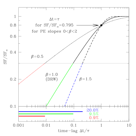
Figure 1: Structure functions (Eqn. (7)) corresponding to three ACFs with the PE power $\beta=0.5$, 1.0 (DRW), and 1.5 (from left to right). The only unbiased measure of the true decorrelation timescale is for the variability amplitude of $0.795~{}SF_{\infty}$. If the timescale is measured at a different amplitude, in this example $0.3~{}SF_{\infty}$ (the gray horizontal line), for $\beta=0.5$ (1.0, 1.5), we in fact measure 0.9% (9.5%, 20%) of the true decorrelation timescale (the bottom inset shows projections of the three SFs below $0.3~{}SF_{\infty}$ onto the time lag axis).

2.1 The Method

It is straightforward to prove that for $\Delta t=\tau$, SF is an unbiased measure (in terms of the underlying process) of the decorrelation timescale, because the exponent then does not depend on $\beta$ and all $0<\beta<2$ SFs cross at the same point (Figure 1). The amplitude of this point is $SF=SF_{\infty}\sqrt{1-\exp(-1)}=0.795~{}SF_{\infty}$. This simply means that once the measured SF reaches the flat part ($SF_{\infty}$) one can just read off the decorrelation timescale from the SF curve and it will be correct for the case of PE ACF regardless of the power.

3 Discussion

Measuring either the SF amplitudes at a fixed timescale (e.g., Vanden Berk et al. 2004; Schmidt et al. 2010; Morganson et al. 2014; Kozłowski et al. 2016) or the timescales at the fixed SF amplitude (e.g., Findeisen et al. 2015; Caplar et al. 2016) are going to provide biased results because the AGN SF slopes at short time lags (or the PSD slopes at high frequencies) are not constant and appear to depend on either the luminosity and/or the black hole mass (Simm et al. 2016; Kozłowski 2016a). If the data are short and/or the break in the SF is not present, however, this is the only justified procedure to be used.

The AGN variability amplitude is known to be anti-correlated with the luminosity (e.g., Angione & Smith 1972; Uomoto et al. 1976; Hook et al. 1994; Paltani & Courvoisier 1994; Giveon et al. 1999). In particular, Kozłowski (2016a) based on the SF analysis of the 9000 SDSS AGNs showed that the SF amplitude at long timescales (the flat part) is $SF_{\infty}\propto L^{-(0.35\pm 0.05)}$. This means that with the increase of brightness by one magnitude the AGN variability amplitude decreases to about 72%. And in fact, the amplitude of the whole SF changes by this amount.

Measuring the decorrelation timescale at a fixed SF amplitude (below $0.795~{}SF_{\infty}$) introduces a bias, because for fainter AGNs with higher variability, the measured decorrelation timescale will appear shorter than the one for the brighter ones, even for the same intrinsic decorrelation timescale (Figure 2, top-left panel). In this example, we measure the time lag at $0.3~{}SF_{\infty}$ (the gray horizontal line). For the faint AGNs (that have set $SF_{\infty}=1.0$ units) we measure 0.094 of the true decorrelation timescale, while for the brighter ones 0.151 (with set $SF_{\infty}=0.8$ units). In other words, when SF is decreasing (along y-axis in Figure 2) because of the increasing $L$, this can be interpreted as a fake increase of $\tau$ (with the increasing $L$) when measuring it at a constant SF level.

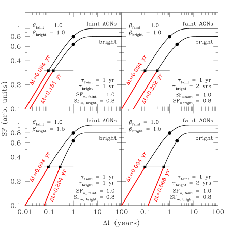
Figure 2: Biases in the decorrelation timescale due to different stochastic processes and the method of measurement. The filled large dots mark the decorrelation timescale at $0.795~{}SF_{\infty}$, while the filled squares show the timescales at the fixed SF amplitude of $0.3~{}SF_{\infty}$ (the gray line). See Section 3 for a detailed discussion.

While there exist an empirical evidence that the decorrelation timescale does not or weakly depend on the AGN luminosity but rather on the black hole mass, $\tau\propto L^{-(0.05\pm 0.17)}M^{(0.38\pm 0.15)}$ from Kozłowski (2016a), the theoretical predictions point to the form $\tau\propto L^{0.5}$ (Frank et al. 2002). In the top-right panel of Figure 2, we show what would happen if the decorrelation timescale had a positive correlation with the luminosity, namely the brighter the AGN the longer the timescale.

Simm et al. (2016) showed that the PSD slope steepens with the increasing black hole mass, and Kozłowski (2016a) showed that the SF slope ($\gamma\equiv\beta/2$) steepens with the increasing luminosity as $\beta\propto L^{(0.10\pm 0.03)}$. In the bottom panels of Figure 2 we include this effect. This causes another bias because the measured time lag at $0.3~{}SF_{\infty}$ increases additionally for bright AGNs. When using the empirically measured relations $SF_{\infty}\propto L^{-0.35}$ and $\beta\propto L^{0.1}$, the measurement of the timescale at a fixed amplitude (below $0.795~{}SF_{\infty}$) produces an artificial relation $\tau\propto L^{\kappa}$ with $0.3\lesssim\kappa\lesssim 0.6$ that is otherwise expected from the theoretical standpoint, namely $\tau\propto L^{0.5}$, and the power of this artificial relation depends on what SF amplitude the $\tau$ measurement is made.

While it is not the goal of this paper to evaluate the biases of the SF amplitude at a fixed timescale, it is easy to decipher from Figure 2 what they would be. If all AGN variability was due to the same process (which is not the case) and the timescale were independent on luminosity (which appears to be the case), the measurement of the SF amplitude would be correct and the amplitude ratio from the bright and faint AGNs would correspond to the ratio of $SF_{\infty}$ for these objects (Figure 2, top-left panel). If we added a theoretical positive correlation of the timescale with the luminosity, the SF amplitude at a fixed timescale would further decrease (Figure 2, top-right panel). Additional decrease will be observed for brighter AGNs because of the steepening of the SF slope (bottom panels of Figure 2). This means that one should seek a relation of $SF_{\infty}$ with the physical AGN parameters and not an arbitrarily selected SF amplitude below the decorrelation timescale, that will be biased.

Obtaining a meaningful SF from a single AGN light curve that typically is short and not well sampled is problematic, if not impossible. Emmanoulopoulos et al. (2010) have already studied and discussed various problems regarding this topic. In particular, they investigate the impact of data sampling and gaps, as well as data length on the SF measurements. The most interesting finding is that for light curves with no intrinsic decorrelation timescales (featureless PSD), breaks will appear in the SFs of almost all light curves, and they provide a rough guide at what timescales they should appear as a function of the experiment length and the PSD slope (their Figure 5). While for all considered types of samplings (dense, sparse, with/without gaps) the short time lag SF part appears to be nearly independent of the sampling, the SFs differ in shape after the spurious break.

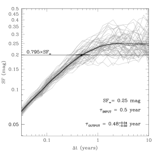
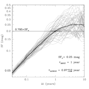
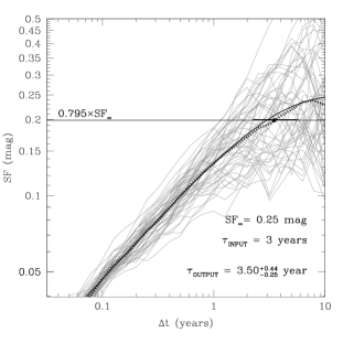
Figure 3: Structure functions for 50 simulated AGN light curves (gray lines) for the same DRW process with $SF_{\infty}=0.25$ mag and $\tau_{\rm INPUT}=0.5$ year (left panel), 1 year (middle), and 3 years (right). The input SF for the DRW process is shown as the black solid line and the ensemble SF is shown as the black dotted line. Emmanoulopoulos et al. (2010) already shown that individual SFs “suffer” from wiggles and/or breaks that are due to the light curve length and cadence. Infinitely long and well-sampled light curves would asymptotically produce the input SFs. A similar effect occurs when one merges a number of individual SFs (the ensemble SF), however, it is not clear if AGNs with similar physical parameters should have the same process leading to variability (although this is commonly assumed). The measured decorrelation timescale $\tau_{\rm OUTPUT}$ is estimated at $0.795~{}SF_{\infty}$ (marked with dot) and can be well-determined from ensemble SFs, provided the data are sufficiently long to constrain $SF_{\infty}$. The horizontal error bar shows the asymmetric one side dispersions, while the reported uncertainties are these dispersions divided by $\sqrt{25}$ (for each side separately).

To explore some of these problems, we simulate three sets of 50 AGN light curves spanning 5000 days (13.7 years) with the same process having $\beta=1.0$, $SF_{\infty}=0.25$ mag, and for the decorrelation timescales of $\tau=0.5$, 1, and 3 years, sampled every 10 days, so having 500 data points (using the prescription from Kozłowski et al. 2010). For every light curve, we calculate its SF (Figure 3, thin gray lines). The SF for the input process is shown as the thick black line in Figure 3. It is obvious that each individual SF differs from the input SF, because of the data sampling and due to different light curve realizations of the same process. We calculate the ensemble SF from the 50 light curves that is shown as the dotted black line in Figure 3. It closely resembles the input SF and we show that the measurement of $\tau$ at $0.795~{}SF_{\infty}$ is adequate (as indicated by the uncertainties). Note, however, we assumed here a simplification by using the exact same process for all 50 light curves (identical process parameters, but different light curve realizations). It is not clear if this assumption holds for the variability processes for a collection of true AGNs with similar physical parameters, although this is what is commonly assumed.

While this question still awaits to be answered, MacLeod et al. (2008) show that ensemble SFs from two-epoch data provide quantitatively similar results to those based on light curves with many epochs.

Another potential problem is mentioned by Emmanoulopoulos et al. (2010), who argued that fitting a model to the SFs is an intrinsically incorrect procedure because the time lag bins are not independent, the SF uncertainties appear too small, and the bootstrap method yields statistically meaningless SF error bars (these problems were also identified and discussed in Kozłowski 2016a). We provide here a method of determination of the decorrelation timescale that is not based on SF fitting, so once the flat part of the SF can be identified, $\tau$ can be just “read off” from the SF at $0.795~{}SF_{\infty}$ level. In practice, however, reaching the $SF_{\infty}$ level may be problematic, because one needs to collect many light curves that are several years long in rest-frame, so for distant AGNs meaning plausibly decades. As already mentioned, also the assumption that an ensemble of light curves for many AGNs can be treated as representative for the group, has not been verified. It is plausible that AGNs with similar or identical physical parameters (the BH mass and luminosity) will have variability that is due to different processes, so ensemble variability studies may not be valid.

Kelly et al. (2011) proposed a sophisticated method of analyzing individual AGN light curves with a mixture of DRW processes, and pointed out that such a mixture can result in a range of PSD slopes. It is likely, however, that most near-future individual light curves will be either short or not well sampled to enable secure determination of the model parameters for large AGN samples, so ensemble SFs will be a must (although see the caveats from the previous paragraph).

4 Summary

In this paper, from basic properties of the covariance of the variable signal in the data, we derived a method of measurement the decorrelation timescale for AGN light curves that always provides the actual and process-independent value. It is valid for SFs that at short time lags show a single power-law behavior and on the long ones appear to be flat, hence the ACF of the process can be of the power exponential type. The decorrelation timescale should be measured at $0.795$ of the SF amplitude at the long timescales (after the photometric noise is removed). We also showed that when using the empirically established relations $SF_{\infty}\propto L^{-0.35}$ and $\beta\propto L^{0.1}$, the measurement of the timescale at a fixed SF amplitude (below $0.795~{}SF_{\infty}$) produces an artificial non-existing relation, $\tau\propto L^{\kappa}$ with $0.3\lesssim\kappa\lesssim 0.6$ (e.g., $\kappa=0.4$ found by Caplar et al. 2016), that is otherwise expected from the theory of accretion disks (i.e., $\kappa\equiv 0.5$).

While individual SFs for typical AGN light curves, that are short and sparsely sampled, are rarely meaningful (Emmanoulopoulos et al. 2010), we showed that ensemble SFs from many AGNs would yield reliable decorrelation timescales for a whole class (having assumed identical variability parameters for individual objects). This is of particular importance because deep, large, optical sky surveys aiming at variability (such as (in the alphabet order) Catalina/CRTS, DES, Gaia, LaSilla-Quest, LSST, OGLE, PanStarrs, and SDSS/BOSS) have already or will provide in the near future light curves for thousands or hundreds of thousands of AGNs. The problem that these data will face, however, is their length and/or cadence. AGNs are typically distant sources with significant redshifts $z$, so the rest frame data lengths, in fact, will be shorter by a factor of $(1+z)$. Such SFs may not probe sufficiently long timescales ($SF_{\infty}$) to measure the decorrelation timescale reliably. Building the ensemble SFs may remain the main tool for these data sets, because the sparseness/length of light curves may prevent their direct modeling (for most of the surveys; see Kozłowski 2016d). The caveat is that the assumption that an ensemble of light curves for many AGNs can be treated as representative for the group has not been verified, but is commonly assumed.

The consecutive SDSS Quasar Data Releases (e.g., Schneider et al. 2010; Pâris et al. 2016) have provided increasingly rich databases of AGN properties that include now $\sim$280,000 black hole mass estimates, the luminosities, and the Eddington ratios (e.g., Shen et al. 2011; Kozłowski 2016c) distributed over a quarter of the sky, enabling unprecedented studies of the connection between the AGN variability and the underlying AGN physics. The forthcoming decades are guaranteed to bring many new and exciting developments in this field of research.

References

- Ackermann et al. (2011) Ackermann, M., Ajello, M., Allafort, A., et al. 2011, ApJ, 743, 171
- Andrae et al. (2013) Andrae, R., Kim, D.-W., & Bailer-Jones, C. A. L. 2013, A&A, 554, A137
- Angione & Smith (1972) Angione, R. J., & Smith, H. J. 1972, External Galaxies and Quasi-Stellar Objects, 44, 171
- Barvainis et al. (2005) Barvainis, R., Lehár, J., Birkinshaw, M., Falcke, H., & Blundell, K. M. 2005, ApJ, 618, 108
- Butler & Bloom (2011) Butler, N. R., & Bloom, J. S. 2011, AJ, 141, 93
- Caplar et al. (2016) Caplar, N., Lilly, S. J., & Trakhtenbrot, B. 2016, arXiv:1611.03082
- Chen & Taam (1995) Chen, X., & Taam, R. E. 1995, ApJ, 441, 354
- Collier & Peterson (2001) Collier, S., & Peterson, B. M. 2001, ApJ, 555, 775
- Czerny (2006) Czerny, B. 2006, Astronomical Society of the Pacific Conference Series, 360, 2
- di Clemente et al. (1996) di Clemente, A., Giallongo, E., Natali, G., Trevese, D., & Vagnetti, F. 1996, ApJ, 463, 466
- Edelson et al. (2014) Edelson, R., Vaughan, S., Malkan, M., et al. 2014, ApJ, 795, 2
- Emmanoulopoulos et al. (2010) Emmanoulopoulos, D., McHardy, I. M., & Uttley, P. 2010, MNRAS, 404, 931
- Findeisen et al. (2015) Findeisen, K., Cody, A. M., & Hillenbrand, L. 2015, ApJ, 798, 89
- Frank et al. (2002) Frank, J., King, A., & Raine, D. J. 2002, Accretion Power in Astrophysics, by Juhan Frank and Andrew King and Derek Raine, pp. 398. ISBN 0521620538. Cambridge, UK: Cambridge University Press, February 2002., 398
- Giveon et al. (1999) Giveon, U., Maoz, D., Kaspi, S., Netzer, H., & Smith, P. S. 1999, MNRAS, 306, 637
- Graham et al. (2014) Graham, M. J., Djorgovski, S. G., Drake, A. J., et al. 2014, MNRAS, 439, 703
- Hook et al. (1994) Hook, I. M., McMahon, R. G., Boyle, B. J., & Irwin, M. J. 1994, MNRAS, 268, 305
- Hughes et al. (1992) Hughes, P. A., Aller, H. D., & Aller, M. F. 1992, ApJ, 396, 469
- Kasliwal et al. (2015a) Kasliwal, V. P., Vogeley, M. S., & Richards, G. T. 2015a, MNRAS, 451, 4328
- Kawaguchi et al. (1998) Kawaguchi, T., Mineshige, S., Umemura, M., & Turner, E. L. 1998, ApJ, 504, 671
- Kelly et al. (2009) Kelly, B. C., Bechtold, J., & Siemiginowska, A. 2009, ApJ, 698, 895
- Kelly et al. (2011) Kelly, B. C., Sobolewska, M., & Siemiginowska, A. 2011, ApJ, 730, 52
- Kelly et al. (2014) Kelly, B. C., Becker, A. C., Sobolewska, M., Siemiginowska, A., & Uttley, P. 2014, ApJ, 788, 33
- King (2008) King, A. 2008, New A Rev., 52, 253
- Kozłowski et al. (2010) Kozłowski, S., Kochanek, C. S., Udalski, A., et al. 2010, ApJ, 708, 927
- Kozłowski et al. (2016) Kozłowski, S., Kochanek, C. S., Ashby, M. L. N., et al. 2016, ApJ, 817, 119
- Kozłowski (2016a) Kozłowski, S. 2016a, ApJ, 826, 118
- Kozłowski (2016b) Kozłowski, S. 2016b, MNRAS, 459, 2787
- Kozłowski (2016c) Kozłowski, S. 2016c, arXiv:1609.09489, ApJS accepted
- Kozłowski (2016d) Kozłowski, S. 2016d, arXiv:1611.08248, A&A accepted
- MacLeod et al. (2008) MacLeod, C., Ivezić, Ž., de Vries, W., Sesar, B., & Becker, A. 2008, American Institute of Physics Conference Series, 1082, 282
- MacLeod et al. (2010) MacLeod, C. L., Ivezić, Ž., Kochanek, C. S., et al. 2010, ApJ, 721, 1014
- MacLeod et al. (2011) MacLeod, C. L., Brooks, K., Ivezić, Ž., et al. 2011, ApJ, 728, 26
- MacLeod et al. (2012) MacLeod, C. L., Ivezić, Ž., Sesar, B., et al. 2012, ApJ, 753, 106
- McHardy et al. (2005) McHardy, I. M., Gunn, K. F., Uttley, P., & Goad, M. R. 2005, MNRAS, 359, 1469
- Morganson et al. (2014) Morganson, E., Burgett, W. S., Chambers, K. C., et al. 2014, ApJ, 784, 92
- Mushotzky et al. (1993) Mushotzky, R. F., Done, C., & Pounds, K. A. 1993, ARA&A, 31, 717
- Mushotzky et al. (2011) Mushotzky, R. F., Edelson, R., Baumgartner, W., & Gandhi, P. 2011, ApJ, 743, L12
- Paltani & Courvoisier (1994) Paltani, S., & Courvoisier, T. J.-L. 1994, A&A, 291, 74
- Pâris et al. (2016) Pâris, I., Petitjean, P., Ross, N. P., et al. 2016, arXiv:1608.06483
- Press et al. (1992a) Press, W. H., Rybicki, G. B., & Hewitt, J. N. 1992a, ApJ, 385, 404
- Press et al. (1992b) Press, W. H., Rybicki, G. B., & Hewitt, J. N. 1992b, ApJ, 385, 416
- Ruan et al. (2012) Ruan, J. J., Anderson, S. F., MacLeod, C. L., et al. 2012, ApJ, 760, 51
- Rybicki & Press (1992) Rybicki, G. B., & Press, W. H. 1992, ApJ, 398, 169
- Scargle (1981) Scargle, J. D. 1981, ApJS, 45, 1
- Scargle (1982) Scargle, J. D. 1982, ApJ, 263, 835
- Scargle (1989) Scargle, J. D. 1989, ApJ, 343, 874
- Schmidt et al. (2010) Schmidt, K. B., Marshall, P. J., Rix, H.-W., Jester, S., Hennawi, J. F., & Dobler, G. 2010, ApJ, 714, 1194
- Schneider et al. (2010) Schneider, D. P., Richards, G. T., Hall, P. B., et al. 2010, AJ, 139, 2360
- Shen et al. (2011) Shen, Y., Richards, G. T., Strauss, M. A., et al. 2011, ApJS, 194, 45
- Siemiginowska & Czerny (1989) Siemiginowska, A., & Czerny, B. 1989, MNRAS, 239, 289
- Simm et al. (2016) Simm, T., Salvato, M., Saglia, R., et al. 2016, A&A, 585, A129
- Simonetti et al. (1984) Simonetti, J. H., Cordes, J. M., & Spangler, S. R. 1984, ApJ, 284, 126
- Simonetti et al. (1985) Simonetti, J. H., Cordes, J. M., & Heeschen, D. S. 1985, ApJ, 296, 46
- Uomoto et al. (1976) Uomoto, A. K., Wills, B. J., & Wills, D. 1976, AJ, 81, 905
- Vagnetti et al. (2016) Vagnetti, F., Middei, R., Antonucci, M., Paolillo, M., & Serafinelli, R. 2016, A&A, 593, A55
- Vanden Berk et al. (2004) Vanden Berk, D. E., Wilhite, B. C., Kron, R. G., et al. 2004, ApJ, 601, 692
- Zu et al. (2011) Zu, Y., Kochanek, C. S., & Peterson, B. M. 2011, ApJ, 735, 80
- Zu et al. (2013) Zu, Y., Kochanek, C. S., Kozłowski, S., & Udalski, A. 2013, ApJ, 765, 106
- Zu et al. (2016) Zu, Y., Kochanek, C. S., Kozłowski, S., & Peterson, B. M. 2016, ApJ, 819, 122