Numerical analysis of an extended structural default model with mutual liabilities and jump risk

Abstract

We consider a structural default model in an interconnected banking network as in Lipton, (2016), with mutual obligations between each pair of banks. We analyse the model numerically for two banks with jumps in their asset value processes. Specifically, we develop a finite difference method for the resulting two-dimensional partial integro-differential equation, and study its stability and consistency. We then compute joint and marginal survival probabilities, as well as prices of credit default swaps (CDS), first-to-default swaps (FTD), credit and debt value adjustments (CVA and DVA). Finally, we calibrate the model to market data and assess the impact of jump risk.

Keywords: structural default model; mutual liabilities; jump-diffusion; finite-difference and splitting methods; calibration.

1 Introduction

The estimation and mitigation of counterparty credit risk has become a pillar of financial risk management. The impact of such risks on financial derivatives is explicitly acknowledged by a valuation adjustment. For an exposition of the background and mathematical models we refer the reader to Gregory, (2012). Although reduced-from models provide for a more direct simulation of default events and are commonly used in financial institutions, we follow here a structural approach which maps the capital structure of a bank into stochastic processes for equity and debt, and models default as the hitting of a lower barrier, as in Black and Cox, (1976). An extensive literature review of further developments of this model is given in Lipton and Sepp, (2013).

A particular concern to regulators and central banks is the impact of default of an entity on the financial system – credit contagion. Of the various channels of such systemic risk described in Hurd, (2016), we focus here on dependencies through asset correlation and interbank liabilities. Specifically, we consider the extended structural default model introduced in Lipton, (2016), where asset values are assumed to follow stochastic processes with correlated diffusion and jump components, and where mutual liabilities can lead to default cascades.

Itkin and Lipton, (2016) consider the model without jumps and obtain explicit expressions for several quantities of interest including the joint and marginal survival probabilities as well as CDSs and FTD prices. They demonstrate that mutual liabilities can have a large impact on the survival probabilities of banks. Thus, a shock of one bank can cause ripples through the whole banking system.

We focus here on the numerical computation of survival probabilities and credit products in the extended model with jumps, where closed-from expressions are no longer available. Our work is therefore most similar to Itkin and Lipton, (2015), who develop a finite difference method for the resulting partial integro-differential equation (PIDE) where the integral term results from a fairly general correlated Levy process in the jump component. By Strang splitting into the diffusion and jump operators, overall second order consistency in the timestep is obtained. Hereby, the multi-dimensional diffusion operator is itself split dimensionwise using the Hundsdorfer-Verwer (HV) scheme, and the jump operator is treated as a pseudo-differential operator, which allows efficient evaluation of the discretised operator by an iterative procedure. Stability of each of the steps is guaranteed under standard conditions.

Our approach is more straightforward in that we apply a modification of the HV scheme directly, where we treat the jump term in the same way as the cross-derivative term in the classical HV scheme. For the analysis we consider infinite meshes, i.e. ignoring the boundaries, such that the discrete operators are also infinite-dimensional. In our analysis we build heavily on the results in In’t Hout and Welfert, (2007) on stability of the PDE with cross-derivatives (but no integral term) and periodic boundary conditions on a finite mesh.

We show that the (unconditional) von Neumann stability of the scheme is not materially affected by the jump operator, as its contribution to the symbol of the scheme is of a lower order in the mesh size. For concreteness, we restrict ourselves to the model with negative exponential jumps described in Lipton, (2016). This allows a simple recursive computation of the discrete jump operator and gives an explicit form of its eigenvalues. However, the analysis can in principle be extended to other jump size distributions.

A survey of splitting methods in finance is found in Toivanen and In’t Hout, (2015). These are roughly arranged in two groups: splitting by dimension (for multi-dimensional PDEs; such as in In’t Hout and Welfert, (2007)), and splitting by operator type (for PIDEs, diffusion and jumps; such as in Andersen and Andreasen, (2000)). Itkin and Lipton, (2015) perform these two splittings successively as described above. To our knowledge, the present paper is the first to perform and analyse splitting into dimensions and jumps simultaneously.

The scheme is constructed to be second order consistent with the continuous integro-differential operator applied to smooth functions. However, the discontinuities in the data lead to empirically observed convergence of only first order in both space and time step. To address this, we apply a spatial smoothing technique discussed in Pooley et al., (2003) for discontinuous option payoffs in the one-dimensional setting, and a change of the time variable to square-root time (see Reisinger and Whitley, (2013)), equivalent to a quadratically refined time mesh close to maturity, in order to restore second order convergence. We emphasise that the presence of discontinuous initial data is essential to the nature of P(I)DE models of credit risk. Hence this approach improves on previous works in a key aspect of the numerical solution.

Similar to Itkin and Lipton, (2016), we restrict the analysis to the two-dimensional case, but there is no fundamental problem in extending the method to multiple dimensions. However, due to the curse of dimensionality, for more than three-dimensional problems, standard finite-difference methods are computationally too expensive. The two-dimensional case already allows us to investigate various important model characteristics, such as joint and marginal survival probabilities, prices of credit derivatives, Credit and Debt Value Adjustments, and specifically the impact of mutual obligations.

In this paper, we consider both unilateral and bilateral counterparty risk as discussed in Lipton and Savescu, (2014). For the unilateral case, the model with two banks is considered, where one is a reference name and the other is either a protection buyer or a protection seller, while for the bilateral case, reference name, protection seller, and protection buyer are considered together, which leads to a three-dimensional problem. We give the equations in the Appendix, but do not include computations.

Moreover, we provide a calibration of the model with negative exponential jumps to market data, and for this calibrated model assess the impact of mutual obligations on survival probabilities.

The novel results of this paper are as follows:

• We analyze a two-dimensional structural default model with interbank liabilities and negative exponential jumps; in particular, we calibrate the model to the market and analyze the impact of jumps on joint and marginal survival probabilities;

• we develop a new finite-difference method to solve the multidimensional PIDE, which is second order consistent in both time and space variables;

• we prove the von Neumann and $l_{2}$ stability of the method;

• we demonstrate empirically that in the presence of discontinuous terminal and boundary conditions, second order of convergence can be maintained by local averaging of the data and suitable refinement of the timestep close to maturity.

The rest of the paper is organized as follows. In Section 2, we formulate the model for two banks with jumps, which is a simplified formulation of Lipton, (2016) for two banks only. Then, we briefly discuss how to compute various model characteristics. In Section 3 we propose a numerical scheme for a general pricing problem; we further prove its stability and consistency. In Section 4 we provide numerical results for various model characteristics computed with the numerical scheme from Section 3. In Section 5 we calibrate the model to the market, and in Section 6 we conclude.

2 Model

We consider the model in Lipton, (2016) for two banks. Assume that the banks have external assets and liabilities, $A_{i}$ and $L_{i}$ respectively, for $i=1,2$, and interbank mutual liabilities $L_{12}$ and $L_{21}$, where $L_{ij}$ is the amount the $i$-th bank owes to the $j$-th bank. Then, the total assets and liabilities for banks 1 and 2 are

$$\tilde{A}_{1}=A_{1}+L_{21},\quad\tilde{L}_{1}=L_{1}+L_{12},$$ (1)

$$\tilde{A}_{2}=A_{2}+L_{12},\quad\tilde{L}_{2}=L_{2}+L_{21}.$$

2.1 Dynamics of assets and liabilities

As in Lipton, (2016), we assume that the firms’ asset values before default are governed by

$$\frac{dA_{i}}{A_{i}}=(\mu-\kappa_{i}\lambda_{i}(t))\,dt+\sigma_{i}\,dW_{i}(t)+(e^{J_{i}}-1)\,dN_{i}(t),\quad i=1,2,$$ (2)

where $\mu$ is the deterministic growth rate, and, for $i=1,2$, $\sigma_{i}$ are the corresponding volatilities, $W_{i}$ are correlated standard Brownian motions,

$$dW_{1}(t)dW_{2}(t)=\rho\,dt,$$ (3)

with correlation $\rho$, $N_{i}$ are Poisson processes independent of $W_{i}$, $\lambda_{i}$ are the intensities of jump arrivals, $J_{i}$ are random negative exponentially distributed jump sizes with probability density function

$$\tilde{\omega}_{i}(s)=\left\{\begin{aligned} &0,&s>0,\\ &\vartheta_{i}e^{\vartheta_{i}s},&s\leq 0,\end{aligned}\right.$$ (4)

with parameters $\vartheta_{i}>0$, and $\kappa_{i}$ are jump compensators

$$\kappa_{i}=\mathbb{E}[e^{J_{i}}-1]=-\frac{1}{\varsigma_{i}+1}.$$ (5)

The jump processes are correlated in the spirit of Marshall and Olkin, (1967). Consider independent Poisson processes $N_{\{1\}}(t),N_{\{2\}}(t)$ and $N_{\{12\}}(t)$, with the corresponding intensities $\lambda_{\{1\}},\lambda_{\{2\}}$ and $\lambda_{\{12\}}$. Then, we define the processes $N_{1}(t)$ and $N_{2}(t)$ as

$$N_{i}(t) =N_{\{i\}}(t)+N_{\{12\}}(t),\qquad i=1,2,$$ (6)

$$\lambda_{i} =\lambda_{\{i\}}+\lambda_{\{12\}},$$

i.e., there are both systemic and idiosyncratic sources of jumps.

We assume that the liabilities are deterministic and have the following dynamics

$$\frac{dL_{i}}{L_{i}}=\mu\,dt,\qquad\frac{dL_{ij}}{L_{ij}}=\mu\,dt,$$ (7)

where $\mu$ is the same growth rate as defined in (2). For pricing purposes, under the risk-neutral measure, we consider $\mu$ as a risk-free short rate. In the following, we take for simplicity $\mu=0$, but the analysis would not change significantly for $\mu\neq 0$.

2.2 Default boundaries

Following Lipton, (2016), we introduce time-dependent default boundaries $\Lambda_{i}(t)$. Bank $i$ is assumed defaulted if its asset value process crosses its default boundary, such that the default time for bank $i$ is

$$\tau_{i}=\inf\{t|\,A_{i}(t)\leq\Lambda_{i}\},\quad i=1,2,$$ (8)

and we define $\tau=\min(\tau_{1},\tau_{2})$.

Before any of the banks $i=1,2$ has defaulted, $t<\tau$,

$$\Lambda_{i}=\left\{\begin{aligned} &R_{i}(L_{i}+L_{i\bar{i}})-L_{\bar{i}i}\equiv\Lambda_{i}^{<},\quad&t<T,\\ &L_{i}+L_{i\bar{i}}-L_{\bar{i}i}\equiv\Lambda_{i}^{=},&t=T,\end{aligned}\right.$$ (9)

where $0\leq R_{i}\leq 1$ is the recovery rate and $\bar{i}=3-i$.

If the $k$-th bank defaults at intermediate time $t$, then for the surviving bank $\bar{k}=3-k$ the default boundary changes to $\Lambda_{\bar{k}}(t+)=\tilde{\Lambda}_{\bar{k}}(t)$, where

$$\tilde{\Lambda}_{\bar{k}}=\left\{\begin{aligned} &R_{\bar{k}}(L_{\bar{k}}+L_{\bar{k}k}-R_{k}L_{k\bar{k}})\equiv\tilde{\Lambda}_{k}^{<},\quad&t<T,\\ &L_{\bar{k}}+L_{\bar{k}k}-R_{k}L_{k\bar{k}}\equiv\tilde{\Lambda}_{i}^{=},&t=T.\end{aligned}\right.$$ (10)

It is clear that for $\Delta\Lambda_{k}(t)\equiv\Lambda_{k}(t+)-\Lambda_{k}(t)$ we have

$$\Delta\Lambda_{k}\equiv\tilde{\Lambda}_{k}-\Lambda_{k}=\begin{cases}(1-R_{\bar{k}}R_{k})L_{k\bar{k}},&t<T,\\ (1-R_{k})L_{k\bar{k}},&t=T.\end{cases}$$ (11)

Thus, $\Delta\Lambda_{k}>0$ and the corresponding default boundaries move to the right. This mechanism can therefore trigger cascades of defaults.

2.3 Terminal conditions

We need to specify the settlement process at time $t=T$. We shall do this in the spirit of Eisenberg and Noe, (2001). Since at time $T$ full settlement is expected, we assume that bank $i$ will pay the fraction $\omega_{i}$ of its total liabilities to creditors. This implies that if $\omega_{i}=1$ the bank pays all liabilities (both external and interbank) and survives. On the other hand, if $0<\omega_{i}<1$, bank $i$ defaults, and pays only a fraction of its liabilities. Thus, we can describe the terminal condition as a system of equations

$$\min\left\{A_{i}(T)+\omega_{\bar{i}}L_{\bar{i}i},L_{i}+L_{i\bar{i}}\right\}=\omega_{i}\left(L_{i}+L_{i\bar{i}}\right).$$ (12)

There is a unique vector $\omega=(\omega_{1},\omega_{2})^{T}$ such that the condition (12) is satisfied. See Lipton, (2016), Itkin and Lipton, (2016) for details.

2.4 Formulation of backward Kolmogorov equation

For convenience, we introduce normalized dimensionless variables

$$\bar{t}=\Sigma^{2}t,\quad X_{i}=\frac{\Sigma}{\sigma_{i}}\ln\left(\frac{A_{i}}{\Lambda_{i}^{<}}\right),\quad\bar{\lambda}_{i}=\frac{\lambda_{i}}{\Sigma^{2}},$$ (13)

where

$$\Sigma=\sqrt{\sigma_{1}\sigma_{2}}.$$

Denote also

$$\xi_{i}=-\left(\frac{\sigma_{i}}{2\Sigma}+\kappa_{i}\bar{\lambda}_{i}\right),\quad\zeta_{i}=\frac{\Sigma}{\sigma_{i}}.$$ (14)

Applying Itô’s formula to $X_{i}$, we find its dynamics

$$dX_{i}=\xi_{i}\,d\bar{t}+dW_{i}(\bar{t})+\zeta_{i}J_{i}\,dN_{i}(\bar{t}).$$ (15)

In the following, we omit bars for simplicity.

The default boundaries change to

$$\mu_{i}=\begin{cases}\mu_{i}^{<}=0,&t<T,\\ \mu_{i}^{=}=\frac{\Sigma}{\sigma_{i}}\ln\left(\frac{\Lambda_{i}^{=}(t)}{\Lambda_{i}^{<}(t)}\right),&t=T.\end{cases}$$ (16)

Assume that the terminal payoff for a contract is $\psi(X_{T})$. Then, the value function is given by

$$V(x,t)=\mathbb{E}\left[\psi(X_{T})\cdot\mathbbm{1}_{\{\tau\geq T\}}+\int_{t}^{T}\chi(s,X_{s})\cdot\mathbbm{1}_{\{\tau>s\}}\,ds\,+\right.\\ \left.+\phi_{1,0}(\tau_{1},X_{2}(\tau_{1}))\cdot\mathbbm{1}_{\{\tau_{1}<T\}}+\phi_{2,0}(\tau_{2},X_{1}(\tau_{2}))\cdot\mathbbm{1}_{\{\tau_{2}<T\}}|\,X(t)=x\right],$$ (17)

where $\chi(\tau,x)$ is the contract payment at an intermediate time $t\leq s\leq T$ (for example, coupon payment), and $\phi_{1,0}(t,X_{2}(t))$ and $\phi_{2,0}(t,X_{1}(t))$ are the payoffs in case of intermediate default of bank 1 or 2, respectively.

Then, according to the Feynman–Kac formula, the corresponding pricing equation is the Kolmogorov backward equation

$$\frac{\partial V}{\partial t}+\mathcal{L}V =\chi(t,x),$$ (18)

$$V(t,0,x_{2}) =\phi_{2,0}(t,x_{1}),\quad V(t,x_{1},x_{2})\underset{x_{1}\to+\infty}{\longrightarrow}\phi_{2,\infty}(t,x_{2}),$$ (19)

$$V(t,x_{1},0) =\phi_{1,0}(t,x_{2}),\quad V(t,x_{1},x_{2})\underset{x_{2}\to+\infty}{\longrightarrow}\phi_{1,\infty}(t,x_{1}),$$ (20)

$$V(T,x) =\psi(x),$$ (21)

where Kolmogorov backward operator

$$\mathcal{L}f=\frac{1}{2}f_{x_{1}x_{1}}+\rho f_{x_{1}x_{2}}+\frac{1}{2}f_{x_{2}x_{2}}+\xi_{1}f_{x_{1}}+\xi_{2}f_{x_{2}}+\lambda_{1}\mathcal{J}_{1}f+\lambda_{2}\mathcal{J}_{2}f+\lambda_{12}\mathcal{J}_{12}f-vf\\ =\Delta_{\rho}f+\xi\cdot\nabla f+\mathcal{J}f-vf,$$ (22)

where $v=\lambda_{1}+\lambda_{2}+\lambda_{12}$ and

$$\mathcal{J}_{1}f(x) =\varsigma_{1}\int_{0}^{x_{1}}f(x_{1}-u,x_{2})e^{-\varsigma_{1}u}du,$$ (23)

$$\mathcal{J}_{2}f(x) =\varsigma_{2}\int_{0}^{x_{2}}f(x_{1},x_{2}-u)e^{-\varsigma_{2}u}du,$$ (24)

$$\mathcal{J}_{12}f(x) =\mathcal{J}_{1}\mathcal{J}_{2}f(x)=\varsigma_{1}\varsigma_{2}\int_{0}^{x_{1}}\int_{0}^{x_{2}}f(x_{1}-u,x_{2}-v)e^{-\varsigma_{1}u-\varsigma_{2}v}dudv,$$ (25)

$\varsigma_{i}=\sigma_{i}\vartheta_{i}/\Sigma$, and $\phi_{i,0},\phi_{i,\infty}$ are given.

In the following, we formulate the Kolmogorov backward equation for specific quantities.

2.5 Joint and marginal survival probabilities

The joint survival probability is the probability that both banks do not default by the terminal time $T$ and given by

$$Q(t,x)=\mathbb{E}[\mathbbm{1}_{\{\tau\geq T,X_{1}(T)\geq\mu_{1}^{=},X_{2}(T)\geq\mu_{2}^{=}\}}\,|X(t)=x].$$ (26)

Then, applying (18)–(21) with $\psi(x)=\mathbbm{1}_{\{x_{1}\geq\mu_{1}^{=},x_{2}\geq\mu_{2}^{=}\}}$ and $\chi(t,x)=0$, we get

$$\frac{\partial Q}{\partial t}+\mathcal{L}Q=0,$$ (27)

$$Q(t,x_{1},0)=0,\quad Q(t,0,x_{2})=0,$$

$$Q(T,x)=\mathbbm{1}_{\{x_{1}\geq\mu_{1}^{=},x_{2}\geq\mu_{2}^{=}\}}.$$

The marginal survival probability for the first bank is the probability that the first bank does not default by the terminal time $T$,

$$q_{1}(t,x)=\mathbb{E}[\mathbbm{1}_{\{\tau\geq T,X_{T}\in D_{1}\cup D_{12})\}}+\Xi(\tau_{2},X_{1}(\tau_{2}))\cdot\mathbbm{1}_{\{\tau_{2}<T\}}|\,X(t)=x],$$ (28)

where $D_{12}$ is the set where both banks survive at the terminal time, $D_{1}$ is the set where only the first bank survives, and $\Xi(\tau_{2},X_{1}(\tau_{2}))$ is the one-dimensional survival probability with the modified boundaries.

Then, applying (18)–(21) with $\psi(x)=\mathbbm{1}_{\{x\in D_{1}\cup D_{12})\}},\chi(t,x)=0$, we get

$$\frac{\partial}{\partial t}q_{1}(t,x)+\mathcal{L}q_{1}(t,x)=0,$$ (29)

$$q_{1}(t,0,x_{2})=0,\quad q_{1}(t,x_{1},0)=\Xi(t,x_{1})=\begin{cases}\chi_{1,0}(t,x_{1}),&x_{1}\geq\tilde{\mu}_{1}^{<},\\ 0,&x_{1}<\tilde{\mu}_{1}^{<},\end{cases}$$

$$q_{1}(t,\infty,x_{2})=1,\quad q_{1}(t,x_{1},\infty)=\chi_{1,\infty}(t,x_{1}),$$

$$q_{1}(T,x)=\mathbbm{1}_{\{x\in D_{1}\cup D_{12}\}}.$$

The function $\chi_{1,0}(t,x_{1})$ is the 1D survival probability, which solves the following boundary value problem

$$\frac{\partial}{\partial t}\chi_{1,0}(t,x_{1})+\mathcal{L}_{1}\chi_{1,0}(t,x_{1})=0,$$ (30)

$$\chi_{1,0}(t,\tilde{\mu}_{1}^{<})=0,\quad\chi_{1,0}(t,\infty)=1,$$

$$\chi_{1,0}(T,x_{1})=\mathbbm{1}_{\{x_{1}>\tilde{\mu}_{1}^{=}\}},$$

where

$$\mathcal{L}_{1}f=\frac{1}{2}\frac{\partial^{2}}{\partial x_{1}^{2}}f+\xi_{1}\frac{\partial}{\partial x_{1}}f+\lambda_{1}\mathcal{J}_{1}f-\lambda_{1}f.$$

Accordingly, $\chi_{1,\infty}(t,x_{1})$ is the 1D survival probability that solves the following boundary value problem

$$\frac{\partial}{\partial t}\chi_{1,\infty}(t,x_{1})+\mathcal{L}_{1}\chi_{1,\infty}(t,x_{1})=0,$$ (31)

$$\chi_{1,\infty}(t,0)=0,\quad\chi_{1,\infty}(t,\infty)=1,$$

$$\chi_{1,\infty}(T,x_{1})=\mathbbm{1}_{\{x_{1}>\mu_{1}^{=}\}}.$$

We formulate the pricing problems for CDS, FTD, CVA and DVA in Appendix A.

3 Numerical scheme

We shall solve the PIDE (18)–(21) numerically with an Alternating Direction Implicit (ADI) method. The scheme is a modification of Lipton and Sepp, (2013) that is unconditionally stable and has second order of convergence in both time and space step.

In order to deal with a forward equation instead of a backward equation, we change the time variable to $\tau=T-t$, so that

$$\frac{\partial V}{\partial\tau}=\mathcal{L}V(\tau,x_{1},x_{2})-\chi(\tau,x_{1},x_{2}),$$ (32)

$$V(\tau,x_{1},0)=\phi_{0,1}(\tau,x_{1}),\quad V(\tau,0,x_{2})=\phi_{0,2}(\tau,x_{2}),$$

$$V(\tau,x_{1},x_{2})\underset{x_{2}\to+\infty}{\longrightarrow}\phi_{\infty,1}(\tau,x_{1}),\quad V(\tau,x_{2},x_{2})\underset{x_{1}\to+\infty}{\longrightarrow}\phi_{\infty,2}(\tau,x_{2}),$$

$$V(0,x_{1},x_{2})=\psi(x_{1},x_{2}).$$

We consider the same grid for integral and differential part of the equation

$$0=x_{1}^{0}<x_{1}^{1}<\ldots<x_{1}^{m_{1}},$$ (33)

$$0=x_{2}^{0}<x_{2}^{1}<\ldots<x_{2}^{m_{2}},$$

where $x_{1}^{m_{1}}$ and $x_{2}^{m_{2}}$ are large positive numbers.

The grid is non-uniform, and is chosen such that relatively many points lie near the default boundaries for better precision. We use a method similar to Itkin and Carr, (2011) to construct the grid.

3.1 Discretization of the integral part of the PIDE

In this section, we shall show how to deal with the integral part of the PIDE, and develop an iterative algorithm for the fast computation of the integral operator on the grid. To this end, we outline the scheme from Lipton and Sepp, (2013) and then give a new method.

The first approach is to deal with the integral operators directly. After the approximation of the integral, we get (Lipton and Sepp, (2013))

$$\mathcal{J}_{1}V(x_{1}+h,x_{2})=e^{-\varsigma_{1}h}\mathcal{J}_{1}V(x_{1},x_{2})+\omega_{0}(\varsigma_{1},h)V(x_{1},x_{2})+\omega_{1}(\varsigma_{1},h)V(x_{1}+h,x_{2})+O(h^{3}),$$ (34)

$$\mathcal{J}_{2}V(x_{1},x_{2}+h)=e^{-\varsigma_{2}h}\mathcal{J}_{2}V(x_{1},x_{2})+\omega_{0}(\varsigma_{2},h)V(x_{1},x_{2})+\omega_{1}(\varsigma_{2},h)V(x_{1},x_{2}+h)+O(h^{3}),$$ (35)

where

$$\omega_{0}(\varsigma,h)=\frac{1-(1+\varsigma h)e^{-\varsigma h}}{\varsigma h},\quad\omega_{1}(\varsigma,h)=\frac{-1+\varsigma h+e^{-\varsigma h}}{\varsigma h}.$$

We can also approximate $\mathcal{J}_{12}V=\mathcal{J}_{1}\mathcal{J}_{2}V$ by applying above approximations for $\mathcal{J}_{1}$ and $\mathcal{J}_{2}$ consecutively.

Consider the grid

$$0=x_{1}^{0}<x_{1}^{1}<\ldots<x_{1}^{m_{1}},$$ (36)

$$0=x_{2}^{0}<x_{2}^{1}<\ldots<x_{2}^{m_{2}},$$

where $x_{1}^{m_{1}}$ and $x_{2}^{m_{2}}$ are large positive numbers.

Then, we can write recurrence formulas for computing the integral operator on the grid. Denote $J_{1}^{i,j},J_{2}^{i,j}$, $J_{12}^{i,j}$ the corresponding approximations of $\mathcal{J}_{1}V(x_{1}^{i},x_{2}^{j})$ , $\mathcal{J}_{2}V(x_{1}^{i},x_{2}^{j})$, $\mathcal{J}_{12}V(x_{1}^{i},x_{2}^{j})$ on the grid. Applying (34) and (35) we get

$$J_{1}^{i+1,j}=e^{-\varsigma_{1}h^{1}_{i+1}}J_{1}^{i,j}+\omega_{0}(\varsigma_{1},h^{1}_{i+1})V(x_{1}^{i},x_{2}^{j})+\omega_{1}(\varsigma_{1},h_{i+1}^{1})V(x_{1}^{i+1},x_{2}^{j}),$$ (37)

$$J_{2}^{i,j+1}=e^{-\varsigma_{2}h^{2}_{j+1}}J_{2}^{i,j}+\omega_{0}(\varsigma_{2},h^{2}_{j+1})V(x_{1}^{i},x_{2}^{j})+\omega_{1}(\varsigma_{2},h_{j+1}^{2})V(x_{1}^{i},x_{2}^{j+1}),$$ (38)

where $h_{i+1}^{1}=x_{1}^{i+1}-x_{1}^{i},h_{j+1}^{2}=x_{2}^{j+1}-x_{2}^{j}$.

For an alternative method, we rewrite the integral operator as a differential equation

$$\frac{\partial}{\partial x_{1}}\left(\mathcal{J}_{1}V(x_{1},x_{2})e^{\varsigma_{1}x_{1}}\right)=\varsigma_{1}V(x_{1},x_{2})e^{\varsigma_{1}x_{1}},$$ (39)

$$\frac{\partial}{\partial x_{2}}\left(\mathcal{J}_{2}V(x_{1},x_{2})e^{\varsigma_{2}x_{2}}\right)=\varsigma_{2}V(x_{1},x_{2})e^{\varsigma_{2}x_{2}},$$ (40)

$$\frac{\partial^{2}}{\partial x_{1}\partial x_{2}}\left(\mathcal{J}_{12}V(x_{1},x_{2})e^{\varsigma_{1}x_{1}+\varsigma_{2}x_{2}}\right)=\varsigma_{1}\varsigma_{2}V(x_{1},x_{2})e^{\varsigma_{1}x_{1}+\varsigma_{2}x_{2}}.$$ (41)

Then, we apply the Adams-Moulton method of second order which gives us third order of accuracy locally (Butcher, (2008))

$$J_{1}^{i+1,j}=e^{-\varsigma_{1}h^{1}_{i+1}}J_{1}^{i,j}+\frac{1}{2}h^{1}_{i+1}e^{-\varsigma_{1}h^{1}_{i+1}}\varsigma_{1}V(x_{1}^{i},x_{2}^{j})+\frac{1}{2}h^{1}_{i+1}\varsigma_{1}V(x_{1}^{i+1},x_{2}^{j}),$$ (42)

$$J_{2}^{i,j+1}=e^{-\varsigma_{2}h^{2}_{j+1}}J_{2}^{i,j}+\frac{1}{2}h^{2}_{j+1}e^{-\varsigma_{2}h^{2}_{j+1}}\varsigma_{2}V(x_{1}^{i},x_{2}^{j})+\frac{1}{2}h^{2}_{j+1}\varsigma_{2}V(x_{1}^{i},x_{2}^{j+1}),$$ (43)

where $h_{i+1}^{1}=x_{1}^{i+1}-x_{1}^{i},h_{j+1}^{2}=x_{2}^{j+1}-x_{2}^{j}$, and is equivalent to the trapezoidal rule.

We can rewrite (42)–(43) in the same notation as (37)–(38) by defining

$$\omega_{0}(\varsigma,h)=\frac{1}{2}he^{-\varsigma h}\varsigma,\quad\omega_{1}(\varsigma,h)=\frac{1}{2}h\varsigma.$$

So,

$$J_{1}^{i+1,j}=e^{-\varsigma_{1}h^{1}_{i+1}}J_{1}^{i,j}+\omega_{0}(\varsigma_{1},h^{1}_{i+1})V(x_{1}^{i},x_{2}^{j})+\omega_{1}(\varsigma_{1},h_{i+1}^{1})V(x_{1}^{i+1},x_{2}^{j}),$$

$$J_{2}^{i,j+1}=e^{-\varsigma_{2}h^{2}_{j+1}}J_{2}^{i,j}+\omega_{0}(\varsigma_{2},h^{2}_{j+1})V(x_{1}^{i},x_{2}^{j})+\omega_{1}(\varsigma_{2},h_{j+1}^{2})V(x_{1}^{i},x_{2}^{j+1}).$$

As a result we get explicit recursive formulas for approximations of $\mathcal{J}_{1}V$ and $\mathcal{J}_{2}V$ that can be computed for all grid points via $O(m_{1}m_{2})$ operations. Both methods give the same order of accuracy. As was discussed above, in order to compute the approximation of $\mathcal{J}_{12}V$ we can apply consecutively the approximations of $\mathcal{J}_{2}V$ and $\mathcal{J}_{1}(\mathcal{J}_{2}V)$. So, we have the two-step procedure:

$$I_{12}^{i+1,j}=e^{-\varsigma_{1}h^{1}_{i+1}}I_{12}^{i,j}+\omega_{0}(\varsigma_{1},h^{1}_{i+1})V(x_{1}^{i},x_{2}^{j})+\omega_{1}(\varsigma_{1},h_{i+1}^{1})V(x_{1}^{i+1},x_{2}^{j}),\\$$ (44)

and

$$J_{12}^{i,j+1}=e^{-\varsigma_{2}h^{2}_{j+1}}J_{12}^{i,j}+\omega_{0}(\varsigma_{2},h^{2}_{j+1})I_{12}^{i,j}+\omega_{1}(\varsigma_{2},h_{j+1}^{2})I_{12}^{i,j+1}.\\$$ (45)

Using this two-step procedure, we can also compute an approximation of $\mathcal{J}_{12}V$ on the grid in complexity $O(m_{1}m_{2})$.

We shall subsequently analyze the stability of the second method and use it in the numerical tests. The results for the first method would be very similar.

For the implementation, computing and storing a matrix representation of the jump operator is not necessary, since the operator can be computed iteratively as described above, but we shall use matrix notation for the analysis. We henceforth denote $J_{1},J_{2}$, and $J_{12}$ the matrices of the discretized jump operators. From (37)–(38) we can find that the matrices $J_{1}$ and $J_{2}$ are lower-triangular with diagonal elements $w_{1}=\omega_{1}(\varsigma_{1},h_{1})$ and $w_{2}=\omega_{1}(\varsigma_{2},h_{2})$. Then, $J_{12}=J_{1}J_{2}$ is also a lower-triangular matrix with diagonal elements $w_{1}w_{2}$. To illustrate, in Figure 1 we plot the sparsity patterns in $J_{1},J_{2}$, and $J_{12}$.

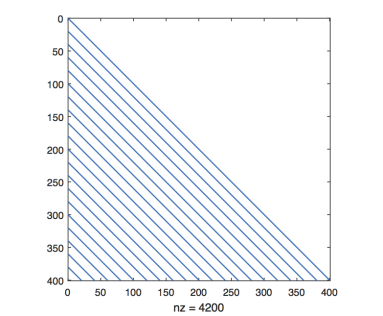
(a) $J_{1}$.

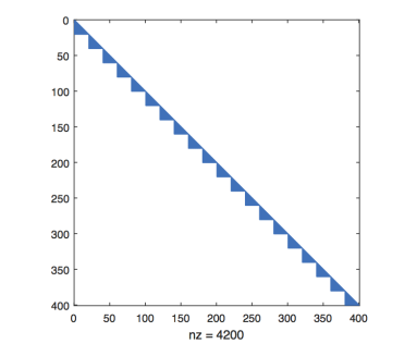
(b) $J_{2}$.

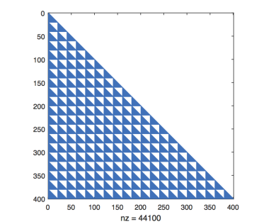
(c) $J_{12}$.

Figure 1: Sparsity pattern of $J_{1}$, $J_{2}$, and $J_{12}$. Here, $m_{1}=m_{2}=20$ and $nz$ is the number of non-zero elements of the matrices.

3.2 Discretization of the differential part of the PIDE

Now consider the approximation of derivatives in the differential operator on a non-uniform grid. We use the standard derivative approximation (Kluge, (2002), In’t Hout and Foulon, (2010)). For the first derivative over each variable consider right-sided, central, and left-sided schemes. So, for the derivative over $x_{1}$ we have:

$$\frac{\partial V}{\partial x_{1}}(x_{1}^{i},x_{2}^{j})\approx\alpha^{1}_{i,-2}V(x_{1}^{i-2},x_{2}^{j})+\alpha^{1}_{i,-1}V(x_{1}^{i-1},x_{2}^{j})+\alpha^{1}_{i,0}V(x_{1}^{i},x_{2}^{j}),$$ (46)

$$\frac{\partial V}{\partial x_{1}}(x_{1}^{i},x_{2}^{j})\approx\beta^{1}_{i,-1}V(x_{1}^{i-1},x_{2}^{j})+\beta^{1}_{i,0}V(x_{1}^{i},x_{2}^{j})+\beta^{1}_{i,1}V(x_{1}^{i+1},x_{2}^{j}),$$ (47)

$$\frac{\partial V}{\partial x_{1}}(x_{1}^{i},x_{2}^{j})\approx\gamma^{1}_{i,0}V(x_{1}^{i},x_{2}^{j})+\gamma^{1}_{i,1}V(x_{1}^{i+1},x_{2}^{j})+\gamma^{1}_{i,2}V(x_{1}^{i+2},x_{2}^{j}),$$ (48)

while for derivative over $x_{2}$ we have:

$$\frac{\partial V}{\partial x_{2}}(x_{1}^{i},x_{2}^{j})\approx\alpha^{2}_{j,-2}V(x_{1}^{i},x_{2}^{j-2})+\alpha^{2}_{j,-1}V(x_{1}^{i},x_{2}^{j-1})+\alpha^{2}_{j,0}V(x_{1}^{i},x_{2}^{j}),$$ (49)

$$\frac{\partial V}{\partial x_{2}}(x_{1}^{i},x_{2}^{j})\approx\beta^{2}_{j,-1}V(x_{1}^{i},x_{2}^{j-1})+\beta^{2}_{j,0}V(x_{1}^{i},x_{2}^{j})+\beta^{2}_{j,1}V(x_{1}^{j},x_{2}^{j+1}),$$ (50)

$$\frac{\partial V}{\partial x_{2}}(x_{1}^{i},x_{2}^{j})\approx\gamma^{2}_{j,0}V(x_{1}^{i},x_{2}^{j})+\gamma^{2}_{j,1}V(x_{1}^{i},x_{2}^{j+1},x_{2}^{j})+\gamma^{2}_{j,2}V(x_{1}^{i},x_{2}^{j+2}),$$ (51)

with coefficients

$$\alpha^{k}_{i,-2} =\frac{\Delta x_{k}^{i}}{\Delta x_{k}^{i-1}(\Delta x_{k}^{i-1}+\Delta x_{k}^{i})}, \alpha^{k}_{i,-1} =\frac{-\Delta x_{k}^{i-1}-\Delta x_{k}^{i}}{\Delta x_{k}^{i-1}\Delta x_{k}^{i}}, \alpha^{k}_{i,0} =\frac{\Delta x_{k}^{i-1}+2\Delta x_{k}^{i}}{\Delta x_{k}^{i}(\Delta x_{k}^{i-1}+\Delta x_{k}^{i})},$$

$$\beta^{k}_{i,-1} =\frac{-\Delta x_{k}^{i+1}}{\Delta x_{k}^{i}(\Delta x_{k}^{i}+\Delta x_{k}^{i+1})}, \beta^{k}_{i,0} =\frac{\Delta x_{k}^{i+1}-\Delta x_{k}^{i}}{\Delta x_{k}^{i}\Delta x_{k}^{i+1}}, \beta^{k}_{i,1} =\frac{\Delta x_{k}^{i}}{\Delta x_{k}^{i+1}(\Delta x_{k}^{i}+\Delta x_{k}^{i+1})},$$

$$\gamma^{k}_{i,0} =\frac{-2\Delta x_{k}^{i+1}-\Delta x_{k}^{i+2}}{\Delta x_{k}^{i+1}(\Delta x_{k}^{i+1}+\Delta x_{k}^{i+2})}, \gamma^{k}_{i,1} =\frac{\Delta x_{k}^{i+1}+\Delta x_{k}^{i+2}}{\Delta x_{k}^{i+1}\Delta x_{k}^{i+2}}, \gamma^{k}_{i,2} =\frac{-\Delta x_{k}^{i+1}}{\Delta x_{k}^{i+2}(\Delta x_{k}^{i+1}+\Delta x_{k}^{i+2})}.$$

For the boundaries at $0$ we use the schemes (46) and (49), for the right boundaries at $x_{1}^{m_{1}}$ and $x_{2}^{m_{2}}$ we use the schemes (48) and (51), and for other points we use the central schemes (47) and (50).

To approximate the second derivative we use the central scheme:

$$\frac{\partial^{2}V}{\partial x_{1}^{2}}(x_{1}^{i},x_{2}^{j})\approx\delta^{1}_{i,-1}V(x_{1}^{i-1},x_{2}^{j})+\delta^{1}_{i,0}V(x_{1}^{i},x_{2}^{j})+\delta^{1}_{i,1}V(x_{1}^{i+1},x_{2}^{j}),$$ (52)

$$\frac{\partial^{2}V}{\partial x_{2}^{2}}(x_{1}^{i},x_{2}^{j})\approx\delta^{2}_{j,-1}V(x_{1}^{i},x_{2}^{j-1})+\delta^{2}_{j,0}V(x_{1}^{i},x_{2}^{j})+\delta^{2}_{j,1}V(x_{1}^{j},x_{2}^{j+1}),$$ (53)

with coefficients

$$\delta^{k}_{i,-1}=\frac{2}{\Delta x_{k}^{i}(\Delta x_{k}^{i}+\Delta x_{k}^{i+1})},\quad\delta^{k}_{i,0}=\frac{-2}{\Delta x_{k}^{i}\Delta x_{k}^{i+1}},\quad\delta^{k}_{i,1}=\frac{2}{\Delta x_{k}^{i+1}(\Delta x_{k}^{i}+\Delta x_{k}^{i+1})},$$

and to approximate the second mixed derivative we use the scheme:

$$\frac{\partial^{2}V}{\partial x_{1}\partial x_{2}}(x_{1}^{i},x_{2}^{j})\approx\sum_{k,l=-1}^{1}\beta_{i,k}^{1}\beta_{j,l}^{2}V(x_{1}^{i+k},x_{2}^{j+l}).$$ (54)

As a result, we can approximate the differential operator $\mathcal{D}V$ by a discrete operator

$$DV=D_{1}V+D_{2}V+D_{12}V,$$ (55)

where $D_{1}V$ contains the discretized derivatives over $x_{1}$ defined in (46)–(48) and (52), $D_{2}V$ contains the discretized derivatives over $x_{2}$ defined in (49)–(51) and (53), and $D_{12}V$ contains the discretized mixed derivative defined in (54).

By straightforward but lengthy Taylor expansion of the expression in (46)–(54), the scheme (59) has second order truncation error in variables $x_{1}$ and $x_{2}$ for meshes which are either uniform or smooth transformations of such meshes, as we shall consider later.

3.3 Time discretization: ADI scheme

After discretization over $(x_{1},x_{2})$ we can rewrite PIDE (32) as a system of ordinary (linear) differential equations. Consider the vector $U(t)\in\mathbb{R}^{m_{1}m_{2}\times 1}$ whose elements correspond to $V(t,x_{1}^{i},x_{2}^{j})$. Then

$$U^{\prime}(t)=\tilde{A}U(t)+b(t),$$ (56)

$$U(0)=U_{0},$$

where $\tilde{A}=D_{1}+D_{2}+D_{12}+\lambda_{1}J_{1}+\lambda_{2}J_{2}+\lambda_{12}J_{12}-(\lambda_{1}+\lambda_{2}+\lambda_{12})I$, and $b(t)$ is determined from boundary conditions and the right-hand side.

To solve this system, we apply an ADI scheme for the time discretization. Consider, for simplicity, a uniform time mesh with time step $\Delta t:t_{n}=n\Delta t,n=0,\ldots,N-1$.

We decompose the matrix $\tilde{A}$ into three matrices, $\tilde{A}=\tilde{A}_{0}+\tilde{A}_{1}+\tilde{A}_{2}$, where

$$\tilde{A}_{0}=D_{12}+\lambda_{1}J_{1}+\lambda_{2}J_{2}+\lambda_{12}J_{12},$$

$$\tilde{A}_{1}=D_{1}-\left(\lambda_{1}+\frac{\lambda_{12}}{2}\right)I,$$

$$\tilde{A}_{2}=D_{2}-\left(\lambda_{2}+\frac{\lambda_{12}}{2}\right)I,$$

and $b(t)=b_{0}(t)+b_{1}(t)+b_{2}(t)$, where $b_{0}(t)$ corresponds to the right-hand side and the FD discretization of the mixed derivatives on the boundary, $b_{1}(t)$ and $b_{2}(t)$ correspond to the FD discretization of the derivatives over $x_{1}$ and $x_{2}$ on the boundary.

Now we can apply a traditional ADI scheme with matrices $\tilde{A}_{0},\tilde{A}_{1}$, and $\tilde{A}_{2}$. We choose the Hundsdorfer–Verwer (HV) scheme (Hundsdorfer and Verwer, (2013)) in order to have second order accuracy in the time variable, and unconditional stability, as we shall prove below. For convenience, denote

$$F_{j}(t,x)=\tilde{A}_{j}x+b_{j}(t),\quad j=0,1,2,$$ (57)

$$F(t,x)=(\tilde{A}_{0}+\tilde{A}_{1}+\tilde{A}_{2})x+(b_{0}(t)+b_{1}(t)+b_{2}(t)),$$ (58)

and apply the Hundsdorfer–Verwer (HV) scheme:

$$\left\{\begin{aligned} &Y_{0}=U_{n-1}+\Delta tF(t_{n-1},U_{n-1}),\\ &Y_{j}=Y_{j-1}+\theta\Delta t(F_{j}(t_{n},Y_{j})-F_{j}(t_{n},U_{n-1})),\quad j=1,2,\\ &\tilde{Y}_{0}=Y_{0}+\sigma\Delta t(F(t_{n},Y_{2})-F(t_{n-1},U_{n-1})),\\ &\tilde{Y}_{j}=\tilde{Y}_{j-1}+\theta\Delta t(F_{j}(t_{n},\tilde{Y}_{j}-F_{j}(t_{n},Y_{2})),\quad j=1,2,\\ &U_{n}=\tilde{Y}_{2}.\end{aligned}\right.$$ (59)

In this scheme, parts that contain $F_{1}$ and $F_{2}$ are treated implicitly. The matrix $\tilde{A}_{1}$ is tridiagonal and $\tilde{A}_{2}$ is block-tridiagonal and can be inverted via $O(m_{1}m_{2})$ operations. As a result, the overall complexity is $O(m_{1}m_{2})$ for a single time step or $O(Nm_{1}m_{2})$ for the whole procedure.

Moreover, the scheme has second order of consistency in both $(x_{1},x_{2})$ and $t$ for any given $\theta$ and $\sigma=\frac{1}{2}$.

3.4 Stability analysis

In this section, we consider the PIDE (32) with zero boundary conditions at $0$ in both directions and on a uniform grid, such that $F_{j}(t,x)=\tilde{A}_{j}x$ and

$$\left\{\begin{aligned} &Y_{0}=U_{n-1}+\Delta t\tilde{A}U_{n-1},\\ &Y_{j}=Y_{j-1}+\theta\Delta t(\tilde{A}_{j}Y_{j}-\tilde{A}_{j}U_{n-1}),\quad j=1,2,\\ &\tilde{Y}_{0}=Y_{0}+\sigma\Delta t(\tilde{A}Y_{2}-\tilde{A}U_{n-1}),\\ &\tilde{Y}_{j}=\tilde{Y}_{j-1}+\theta\Delta t(\tilde{A}_{j}\tilde{Y}_{j}-\tilde{A}_{j}Y_{2}),\quad j=1,2\\ &U_{n}=\tilde{Y}_{2}.\end{aligned}\right.$$ (60)

For convenience, we denote by $F:U_{n}=FU_{n-1}$.

We further consider the PDE on $\mathbb{R}^{2}$, i.e., without default boundaries. Hence, we assume that diffusion and jump operators are discretized on an infinite, uniform mesh $\{(j_{1}h_{1},j_{2}h_{2}),(j_{1},j_{2})\in\mathbb{Z}^{2}\}$, such that, e.g. $D_{1},D_{2},D_{12},J_{1},J_{2}$ are infinite matrices. This is different to In’t Hout and Welfert, (2007), where finite matrices and periodic boundary conditions (without integral terms) are considered.

We use von Neumann stability analysis, as first introduced by Charney et al., (1950), by expanding the solution into a Fourier series. Hence, we shall show that the proposed scheme (60) is unconditionally stable, i.e. we will show that all eigenvalues of the operator $F$ have moduli bounded by 1 plus an $O(\Delta t)$ term, where the corresponding eigenfunctions are given by $\exp(i\phi_{1}j_{1})\exp(i\phi_{2}j_{2})$, with $\phi_{1}$ and $\phi_{2}$ the wave numbers and $j_{1}$ and $j_{2}$ the grid coordinates.

In’t Hout and Welfert, (2007) show that when all matrices commute (as in the PDE case with periodic boundary conditions), the eigenvalues for $F$ are given by

$$T(\tilde{z}_{0},\tilde{z}_{1},\tilde{z}_{2}) = 1+2\frac{\tilde{z}_{0}+\tilde{z}}{p}-\frac{\tilde{z}_{0}+\tilde{z}}{p^{2}}+\sigma\frac{(\tilde{z}_{0}+\tilde{z})^{2}}{p^{2}}\quad\text{with}$$ (61)

$$p = (1-\theta\tilde{z}_{1})(1-\theta\tilde{z}_{2}),$$

where $\tilde{z}_{j}=\tilde{\mu}_{j}\Delta t$, where $\tilde{\mu}_{j}$ is an eigenvalue of $\tilde{A}_{j}$, $j=0,1,2$, $\tilde{z}=\tilde{z}_{1}+\tilde{z}_{2}$, $\theta\geq 0$.

The analysis is made slightly more complicated in our case through the presence of the jump operators. In the remainder of this section, we show that stability is still given under the same conditions on $\theta$ and $\sigma$ as in the purely diffusive case. For the correspondence of notation with In’t Hout and Welfert, (2007), we denote $A=A_{0}+A_{1}+A_{2}$, where $A_{0}=D_{12},A_{1}=D_{1}$, $A_{2}=D_{2}$ and $\mu_{0},\mu_{1}$, and $\mu_{2}$ are the eigenvalues of the corresponding matrices. Similar to $\tilde{z}_{0},\tilde{z}_{1},$ and $\tilde{z}_{2}$, we define scaled eigenvalues $z_{0}=\mu_{0}\Delta t,z_{1}=\mu_{1}\Delta t,z_{2}=\mu_{2}\Delta t$.

We have the eigenvalues $\tilde{\mu}_{j}$ of $\tilde{A}_{j}$ given by

$$\tilde{\mu}_{0}=\mu_{0}+\lambda_{1}w_{1}+\lambda_{2}w_{2}+\lambda_{12}w_{12},$$ (62)

$$\tilde{\mu}_{1}=\mu_{1}-\left(\lambda_{1}+\frac{\lambda_{12}}{2}\right),$$ (63)

$$\tilde{\mu}_{2}=\mu_{2}-\left(\lambda_{2}+\frac{\lambda_{12}}{2}\right),$$ (64)

where $\mu_{j}$ is an eigenvalue of $A_{j}$, and $w_{1},w_{2}$, and $w_{12}$ are eigenvalues of $J_{1},J_{2}$, and $J_{12}$.

Denote $z=z_{1}+z_{2}$, $s_{1}=w_{1}\Delta t,s_{2}=w_{2}\Delta t,s_{12}=w_{12}\Delta t$, where $w_{1},w_{2},w_{12}$ are eigenvalues of $J_{1},J_{2},J_{12}$ respectively, and $s_{0}=\lambda_{1}s_{1}+\lambda_{2}s_{2}+\lambda_{12}s_{12}$.

Multiplying (62)–(64) by $\Delta t$, we have

$$\tilde{z}_{0}=z_{0}+s_{0},$$ (65)

$$\tilde{z}_{1}=z_{1}-\left(\lambda_{1}+\frac{\lambda_{12}}{2}\right)\Delta t,$$ (66)

$$\tilde{z}_{2}=z_{2}-\left(\lambda_{2}+\frac{\lambda_{12}}{2}\right)\Delta t.$$ (67)

Theorem 1 (In’t Hout and Welfert, (2007), Theorem 3.2).

Assume $\Re({z}_{1})\leq 0,\Re({z}_{2})\leq 0$, $|{z}_{0}|\leq 2\sqrt{\Re({z}_{1})\Re({z}_{2})}$, where ${z}_{0},{z}_{1}$, and ${z}_{2}$ are the eigenvalues of ${A}_{0},{A}_{1}$, and ${A}_{2}$, and

$$\frac{1}{2}\leq\sigma\leq\left(1+\frac{\sqrt{2}}{2}\right)\theta.$$

Then,

$$|T({z}_{0},{z}_{1},{z}_{2})|\leq 1,$$

and the Hundsdorfer–Verwer scheme (60) is stable in the purely diffusive case.

Lemma 1.

The scaled eigenvalues of $A_{0}$, $A_{1}$, $A_{2}$, $J_{1}$, $J_{2}$, $J_{12}$ can be expressed as

$$z_{0} = -\rho b[\sin{\phi_{1}}\sin{\phi_{2}}],$$ (68)

$$z_{1} = -a_{1}(1-\cos{\phi_{1}})+i\xi_{1}q_{1}\sin{\phi_{1}},$$ (69)

$$z_{2} = -a_{2}(1-\cos{\phi_{2}})+i\xi_{2}q_{2}\sin{\phi_{2}},$$ (70)

$$s_{1} = \Delta t\,\zeta_{1}h_{1}\left(\frac{1}{2}+\frac{\exp(-h_{1}\zeta_{1}+i\phi_{1})}{1-\exp(-h_{1}\zeta_{1}+i\phi_{1})}\right),$$ (71)

$$s_{2} = \Delta t\,\zeta_{2}h_{2}\left(\frac{1}{2}+\frac{\exp(-h_{2}\zeta_{2}+i\phi_{2})}{1-\exp(-h_{2}\zeta_{2}+i\phi_{2})}\right),$$ (72)

$$s_{12} = s_{1}s_{2}/\Delta t,$$ (73)

where

$$q_{1}=\frac{\Delta t}{h_{1}},\quad q_{2}=\frac{\Delta t}{h_{2}},\quad a_{1}=\frac{\Delta t}{h_{1}^{2}},\quad a_{2}=\frac{\Delta t}{h_{2}^{2}},\quad b=\frac{\Delta t}{h_{1}h_{2}},$$

and $\phi_{j}\in[0,2\pi]$ for $j=1,2$.

Moreover,

$$|z_{0}|\leq 2\sqrt{\Re(z_{1})\Re(z_{2})}.$$ (74)

Proof.

All six eigenvalues follow by insertion of the ansatz $U=\exp(i\phi_{1}j_{1})\exp(i\phi_{2}j_{2})$. For instance,

$$(J_{1}U)(j_{1},j_{2})=\zeta_{1}h_{1}\left(\frac{1}{2}U(j_{1},j_{2})+\sum_{k=1}^{\infty}\exp(-\zeta_{1}h_{1}k)U(j_{1}-k,j_{2})\right),$$

and the result follows by using the special form of $U$ and evaluating the geometric series.

Alternatively, the first three equations follow immediately from the eigenvalues for finite matrices (In’t Hout and Welfert, (2007), p.29), which are given by (68)–(70) where $\phi_{j}=2l\pi/m_{j}$, $l=1,\ldots,m_{j}$. In the infinite mesh case, the spectrum is the continuous limit and (74) still holds. ∎

Theorem 2.

Consider $\frac{1}{2}\leq\sigma\leq\left(1+\frac{\sqrt{2}}{2}\right)\theta$. Then there exists $c>0$, independent of $\Delta t\leq 1$, $h_{1}$ and $h_{2}$, such that

1. $$|T(\tilde{z}_{0},\tilde{z}_{1},\tilde{z}_{2})|\leq 1+c\Delta t,\qquad\forall\phi_{1},\phi_{2}\in[0,2\pi],$$ (75)

   i.e., the scheme is von Neumann stable;

2. $$|U_{n}|_{2}\leq{\rm e}^{cn\Delta t}|U_{0}|_{2},\qquad\forall n\geq 0,$$ (76)

   for $|U_{n}|_{2}=h_{1}h_{2}\left(\sum_{j_{1},j_{2}=-\infty}^{\infty}|U_{n}(j_{1},j_{2})|^{2}\right)^{\scriptsize 1/2}$, i.e., the scheme is $l_{2}$ stable.

Proof.

First, we have that

$$|T({z}_{0},\tilde{z}_{1},\tilde{z}_{2})|=\left|1+2\frac{{z}_{0}+\tilde{z}}{p}-\frac{{z}_{0}+\tilde{z}}{p^{2}}+\sigma\frac{({z}_{0}+\tilde{z})^{2}}{p^{2}}\right|\leq 1,$$

where as before $p=(1-\theta\tilde{z}_{1})(1-\theta\tilde{z}_{2})$ and $\tilde{z}=\tilde{z}_{1}+\tilde{z}_{2}$. This follows from Theorem 1 because $\lambda_{1}$, $\lambda_{2}$ and $\lambda_{12}$ are positive and therefore (74) is still satisfied with $z_{1}$ and $z_{2}$ replaced by $\tilde{z}_{1}$ and $\tilde{z}_{2}$.

We have

$$T(\tilde{z}_{0},\tilde{z}_{1},\tilde{z}_{2}) = T({z}_{0},\tilde{z}_{1},\tilde{z}_{2})+2\frac{s_{0}}{p}-\frac{s_{0}}{p^{2}}+\sigma\frac{2s_{0}(z_{0}+\tilde{z})+s_{0}^{2}}{p^{2}}.$$

A simple calculation shows that $|s_{0}|\leq c_{0}\,\Delta t$ for a constant $c_{0}$ (independent of $\Delta t,h_{1},h_{2},\phi_{1}$, $\phi_{2}$; indeed, $c_{0}=2\lambda_{1}+2\lambda_{2}+4\lambda_{12}$ works for small enough $h_{1}$, $h_{2}$). Therefore, and because $|p|\geq 1$, $|z_{0}+\tilde{z}|/|p|\leq c_{1}$ for a constant $c_{1}$,

$$\left|2\frac{s_{0}}{p}-\frac{s_{0}}{p^{2}}+\sigma\frac{2s_{0}(z_{0}+\tilde{z})+s_{0}^{2}}{p^{2}}\right|\leq c\Delta t,$$

for any $c\geq(3+2\sigma c_{1}+c_{0}\sigma)c_{0}$. From this the first statement follows.

We can now deduce part 2 by a standard argument. For the discrete-continuous Fourier transform

$$l_{2}(\mathbb{Z}^{2})\rightarrow L_{2}(-\pi,\pi)^{2},\qquad U\rightarrow\widehat{U},\qquad\widehat{U}(\phi_{1},\phi_{2})=h_{1}h_{2}\sum_{j,k\in\mathbb{Z}}U(j,k){\rm e}^{-i(j\phi_{1}+k\phi_{2})},$$

we have

$$\widehat{U}_{n+1}(\phi_{1},\phi_{2})=T(\tilde{z}_{0},\tilde{z}_{1},\tilde{z}_{2})\,\widehat{U}_{n}(\phi_{1},\phi_{2}),\qquad\forall n\geq 0.$$

Then, by Parseval,

$$|U_{n}|_{2}^{2} = \frac{1}{4\pi^{2}}|\widehat{U}_{n}|^{2}$$

$$= \frac{1}{4\pi^{2}}\frac{1}{h_{1}^{2}h_{2}^{2}}\int_{-\pi}^{\pi}|\widehat{U}_{n}(\phi_{1},\phi_{2})|^{2}\,{\rm d}\phi_{1}\,{\rm d}\phi_{2}$$

$$\leq \frac{1}{4\pi^{2}}\frac{1}{h_{1}^{2}h_{2}^{2}}\int_{-\pi}^{\pi}(1+c\Delta t)^{2n}|\widehat{U}_{0}(\phi_{1},\phi_{2})|^{2}\,{\rm d}\phi_{1}\,{\rm d}\phi_{2}$$

$$\leq {\rm e}^{2cn\Delta t}\frac{1}{4\pi^{2}}\frac{1}{h_{1}^{2}h_{2}^{2}}\int_{-\pi}^{\pi}|\widehat{U}_{0}(\phi_{1},\phi_{2})|^{2}\,{\rm d}\phi_{1}\,{\rm d}\phi_{2}$$

$$= {\rm e}^{2cn\Delta t}|U_{0}|_{2}^{2}.$$

∎

This ($l_{2}$-)stability result together with second order consistency implies ($l_{2}$-)convergence of second order for all solutions which are sufficiently smooth that the truncation error is defined and bounded. In our setting, where the initial condition is discontinuous, this is not given. Since the step function lies in the ($l_{2}$-)closure of smooth functions, convergence is guaranteed, but usually not of second order. We show this empirically in the next section and demonstrate how second order convergence can be restored practically.

3.5 Discontinuous boundary and terminal conditions

It is well documented (see, e.g. Pooley et al., (2003)) that the spatial convergence order of central finite difference schemes is generally reduced to one for discontinuous payoffs. Moreover, the time convergence order of the Crank-Nicolson scheme is reduced to one due to the lack of damping of high-frequency components of the error, and this behaviour is inherited by the HV scheme. We address these two issues in the following way.

First, we smooth the terminal condition by the method of local averaging from Pooley et al., (2003), i.e., instead of using nodal values of $\phi$ directly, we use the approximation

$$\phi(x_{1}^{i},x_{2}^{j})\approx\frac{1}{h_{1}h_{2}}\int_{x_{2}^{i}-h_{2}/2}^{x_{2}^{i}+h_{2}/2}\int_{x_{1}^{j}-h_{1}/2}^{x_{1}^{j}+h_{1}/2}\phi(\xi_{1},\xi_{2})\,d\xi_{1}d\xi_{2}.$$

For step functions with values of 0 and 1, this procedure attaches to each node the fraction of the area where the payoff is 1, in a cell of of size $h_{1}\times h_{2}$ centred at this point.

We illustrate the convergence improvement on the example of joint survival probabilities. Other quantities show a similar behaviour. The model parameters in the following tests are the same as in the next section, specifically Table 1.

We choose $\sigma=\frac{1}{2}$ and $\theta=\frac{3}{4}$ in the HV scheme.

The observed convergence with and without this smoothing procedure is shown in Figure 2. We choose the $l_{2}$-norm for its closeness to the stability analysis – in the periodic case, Fourier analysis gives convergence results in $l_{2}$ – and the $l_{\infty}$-norm for its relevance to the problem at hand, where we are interested in the solution pointwise. The behaviour in the $l_{1}$-norm is very similar.

Hereby, for a method of order $p\geq 1$ we estimate the error by extrapolation as

$$|Q^{nX}(x_{1},x_{2})-Q(x_{1},x_{2})|\approx\frac{1}{2^{p}-1}|Q^{nX}(x_{1},x_{2})-Q^{nX/2}(x_{1},x_{2})|,$$

where $Q$ is the exact solution, $Q^{nX}$ the solution with $nX$ mesh points, and the norms are computed by either taking the maximum over mesh points or numerical quadrature. Here, $nT=1000$ is fixed.

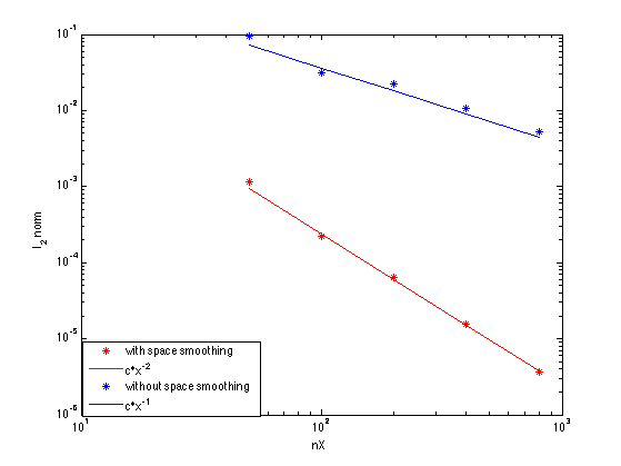
(a) $l_{2}$-norm.

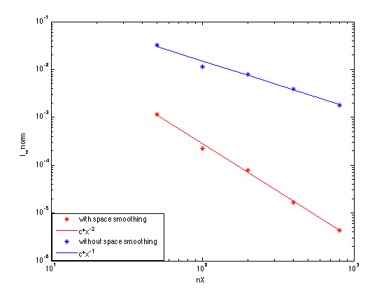
(b) $l_{\infty}$-norm.

Figure 2: Convergence analysis for $l_{2}$- and $l_{\infty}$-norms of the error depending on the mesh size with fixed time-step.

The convergence is clearly of first order without averaging and of second order with averaging.

Second, we modify the scheme using the idea from Reisinger and Whitley, (2013) by changing the time variable $\tilde{t}=\sqrt{t}$. This change of variables leads to the new PDE

$$\frac{\partial V}{\partial\tilde{t}}+2\tilde{t}\mathcal{L}V=2\tau\chi(\tilde{t}^{2},x),$$

instead of (18), to which we apply the numerical scheme.

In Figure 3, we show the convergence with and without time change, estimating the errors in a similar way to above, with $nX=800$ fixed.

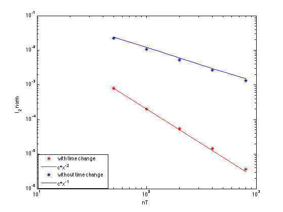
(a) $l_{2}$-norm.

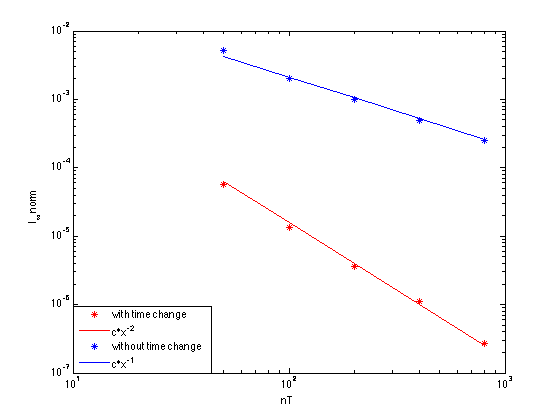
(b) $l_{\infty}$-norm.

Figure 3: Convergence analysis for $l_{2}$- and $l_{\infty}$-norms of the error depending on time-step with fixed mesh size.

The convergence is clearly of first order without time change and of second order with time change. We took here $T=5$ to illustrate the effect more clearly.

4 Numerical experiments

In this section, we analyze the model characteristics and the impact of jumps. Specifically, we compute joint and marginal survival probabilities, CDS and FTD spreads as well as CVA and DVA depending on initial asset values. We also compute the difference between the solution with and without jumps.

Consider the parameters in Table 1.

$L_{1,0}$	$L_{2,0}$	$L_{12,0}$	$L_{21,0}$	$R_{1}$	$R_{2}$	$T$	$\sigma_{1}$	$\sigma_{2}$	$\rho$	$\varsigma_{1}$	$\varsigma_{2}$
60	70	10	15	0.4	0.45	1	1	1	0.5	1	1

Table 1: Model parameters.

For the model with jumps, we further consider the parameters in Table 2.

$\lambda_{1}$	$\lambda_{2}$	$\lambda_{12}$
0.5	0.5	0.3

Table 2: Jump intensities.

We compute all tests using a $100\times 100$ spatial grid with the maximum values $X_{1}^{100}=X_{2}^{100}=10$ and constant time step $\Delta\tau=0.01$. As the parameters of the HV scheme, we choose $\sigma=\frac{1}{2}$ and $\theta=\frac{3}{4}$.

In Figures 4–6 we present various model characteristics and compare the results with and without jumps. From these figures, we can observe that jumps can have a significant impact, especially near the default boundaries:

• in Figure 4 for the joint survival probability, the biggest impact of jumps is around the default boundaries for both $x_{1}$ and $x_{2}$;

• in Figure 5 for the marginal survival probability of the first bank, we can observe that the biggest impact of jumps is near the default boundary of the first bank;

• for the CDS spread, in Figure 6, (b), the biggest impact of jumps is also seen near the default boundary, but it has the opposite direction, because jumps can only increase the CDS spread;

• in Figure 6, (d) for FTD the spread, the biggest impact of jumps is near both default boundaries, and it has a positive impact;

• finally, for CVA, (f), the highest impact of jumps is near the default boundary of the first bank, see Figure 6.

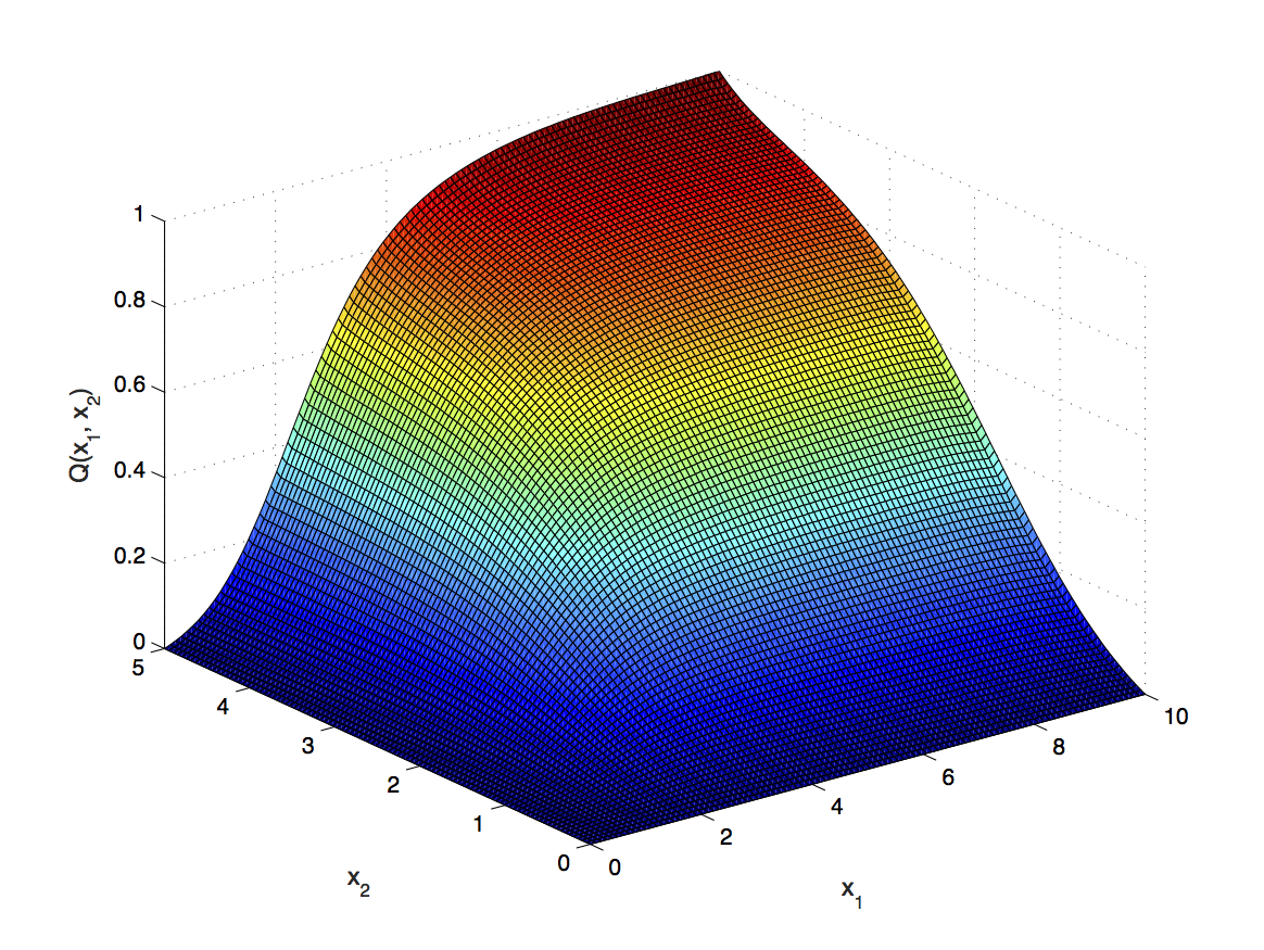
(a)

(b)

Figure 4: The joint survival probability: (a) value, (b) difference between model with and without jumps.

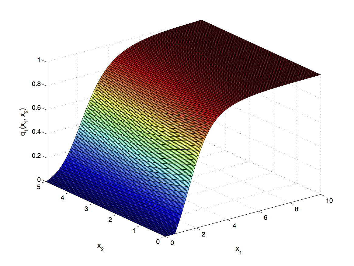
(a)

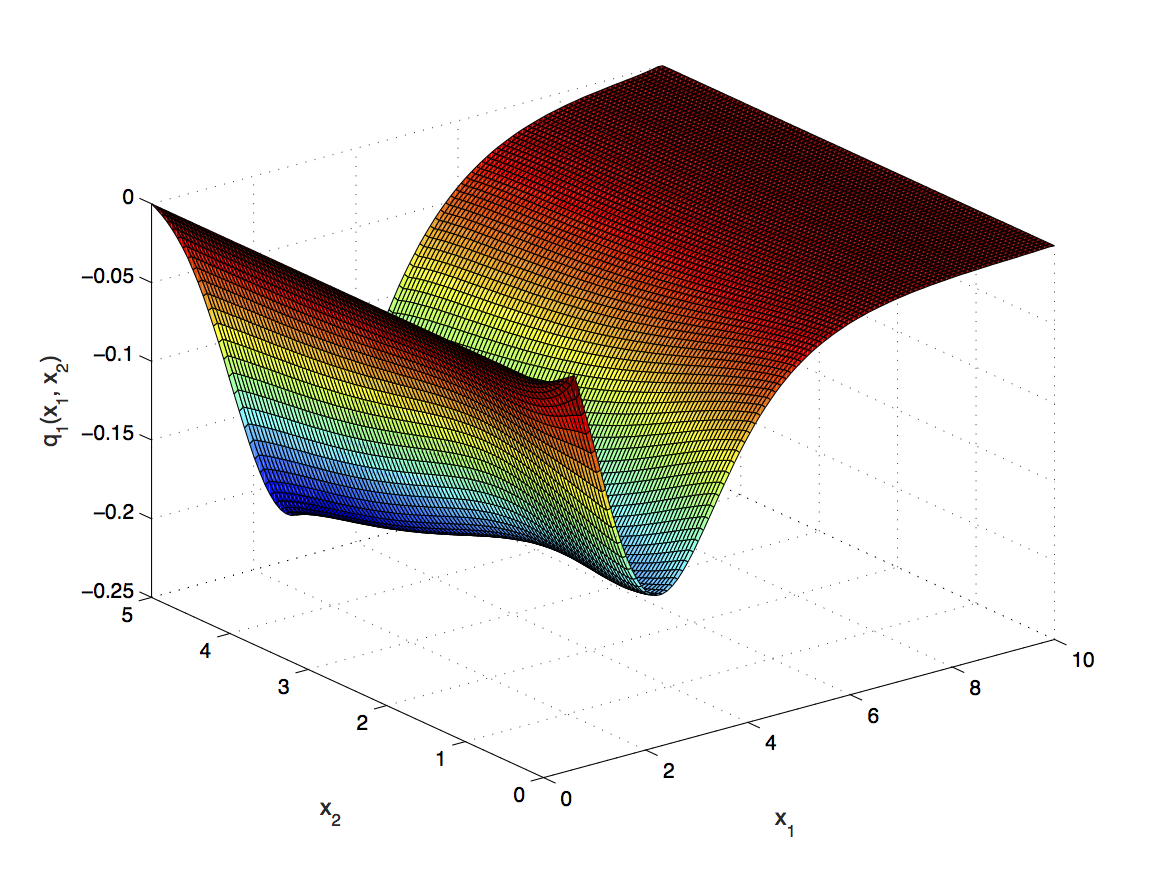
(b)

Figure 5: The marginal survival probability: (a) value, (b) difference between model with and without jumps.

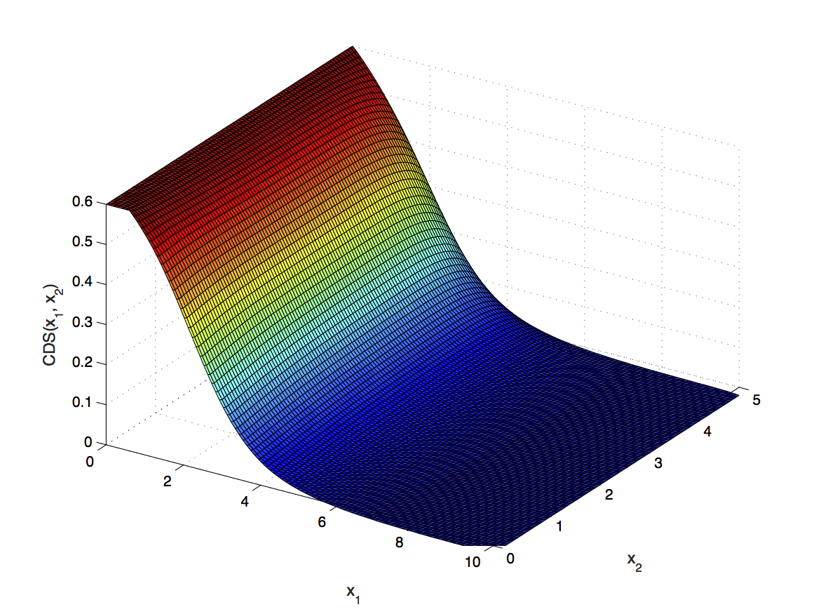
(a)

(b)

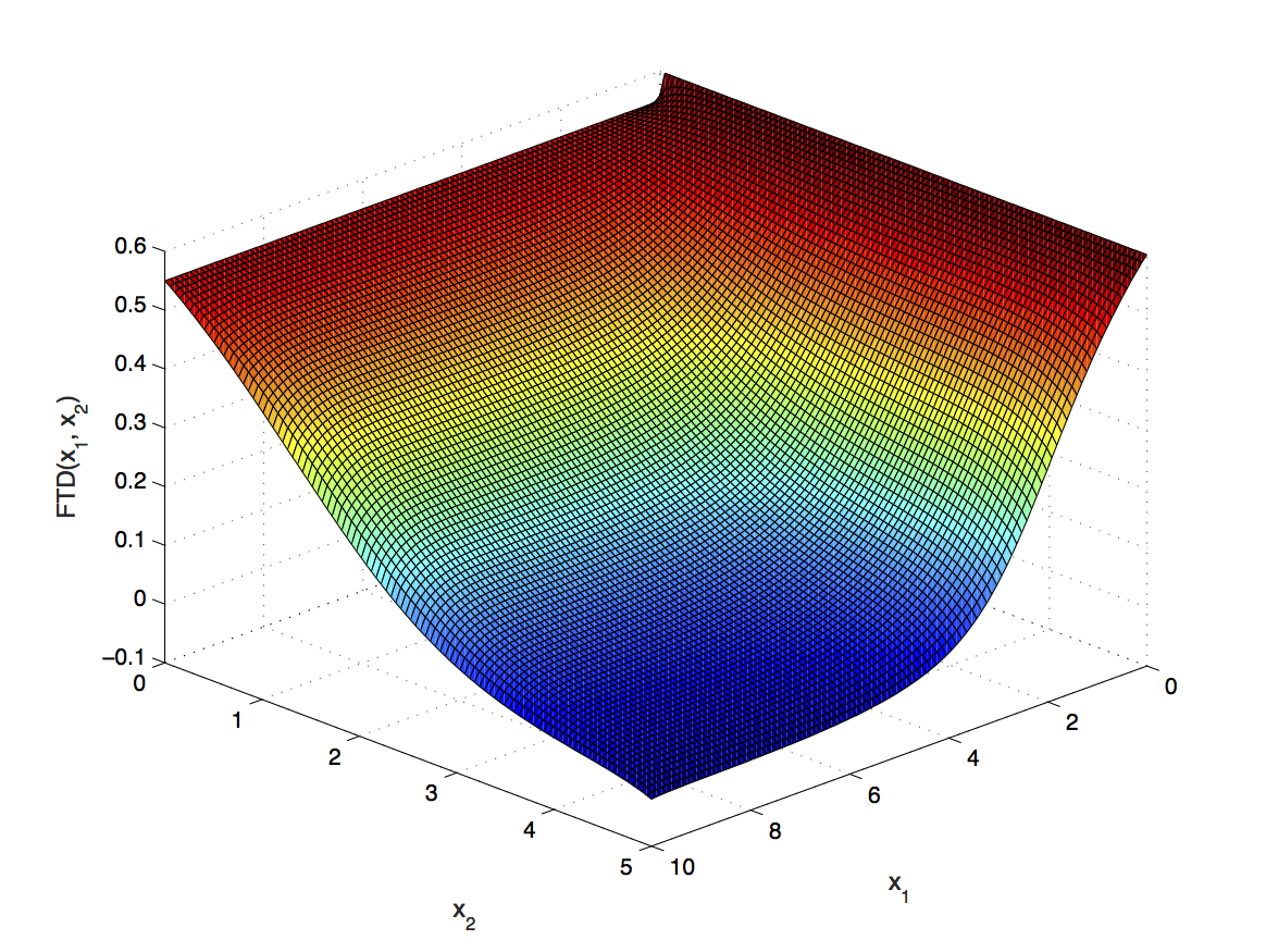
(c)

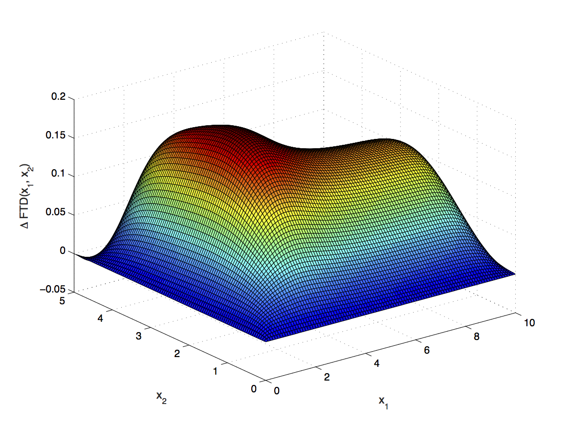
(d)

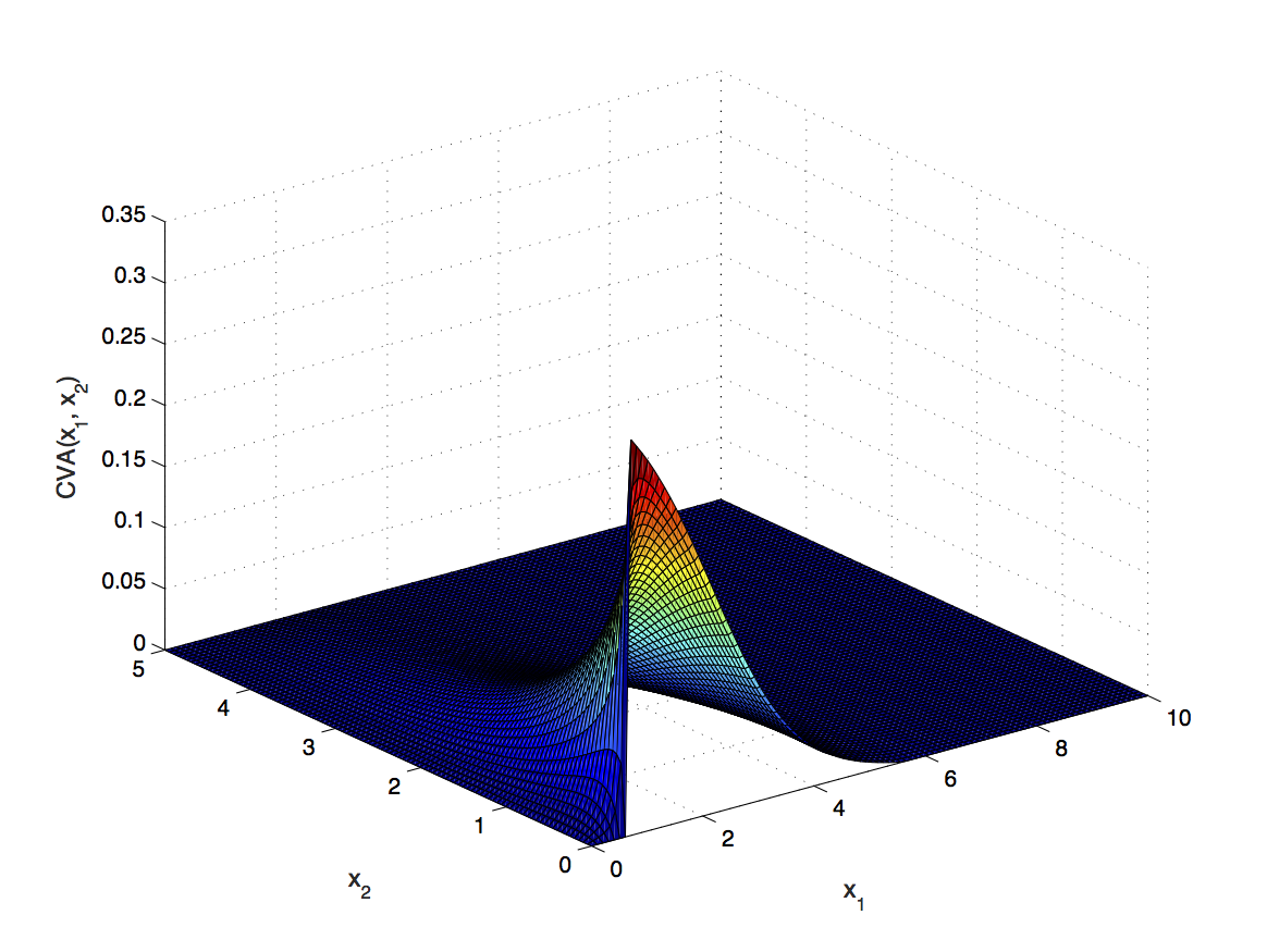
(e)

(f)

Figure 6: Values of different credit products with left the value and right the difference between model with and without jumps. Top row: Credit Default Swap spread, written on the first bank. Middle row: First-to-Default spread. Bottom row: CVA of CDS, where the first bank is Reference name (RN) and the second bank is Protection Seller (PS).

5 Calibration

In this section we present calibration results of the model. There are eight unknown parameters, see (22)–(25): $\sigma_{1},\sigma_{2},\rho,\varsigma_{1},\varsigma_{2},\lambda_{1},\lambda_{2},\lambda_{12}$. We use CDS and equity put option prices (with different strikes) as market data. If FTD contracts are available, one can use them to estimate $\rho$ and $\lambda_{12}$. Otherwise, historical estimation with share prices time series can be used.

The data for external liabilities can be found in banks’ balance sheets, which are publicly available. Usually, mutual liabilities data are not public information, thus we made an assumption that they are a fixed proportion of the total liabilities, which coincides with David and Lehar, (2014). In particular, we fix the mutual liabilities as 5% of total liabilities.

The asset’s value is the sum of liabilities and equity price.

We choose Unicredit Bank as the first bank and Santander as the second bank. In Table 3 we provide their equity price $E_{i}$, assets $A_{i}$ and liabilities $L_{i}$. As in Lipton and Sepp, (2013), the liabilities are computed as a ratio of total liabilities and shares outstanding.

$E_{1}(0)$	$L_{1}(0)$	$A_{1}(0)$	$E_{2}(0)$	$L_{2}(0)$	$A_{2}(0)$
6.02	137.70	143.72	6.23	86.41	92.64

Table 3: Assets and liabilities on 30/06/2015 (Bloomberg).

For the calibration we choose 1-year at-the-money, in-the-money, and out-of-the-money equity put options on the banks, and 1-year CDS contracts. Since the spreads of CDS are usually significantly lower than the option prices, we scale them by some weight $w_{i}$ in the objective function. As a result, we have the following 6-dimensional minimization problem:

$$\min_{\theta}\{w_{1}(V^{CDS}_{1}(\theta)-\bar{V}^{CDS}_{1})^{2}+\sum\limits_{i=1}^{3}(V^{opt}_{1}(K_{i,1},\theta)-\bar{V}^{opt}_{1}(K_{i,1}))^{2}+\\ +w_{2}(V^{CDS}_{2}(\theta)-\bar{V}^{CDS}_{2})^{2}+\sum\limits_{i=1}^{3}(V^{opt}_{2}(K_{i,2},\theta)-\bar{V}^{opt}_{2}(K_{i,2}))^{2}\},$$ (77)

where $\theta=(\sigma_{1},\sigma_{2},\lambda_{1},\lambda_{2},\varsigma_{1},\varsigma_{2})$, $V^{CDS}_{i}(\theta)$ is the model CDS spread on the $i$-th bank and $\bar{V}^{CDS}_{i}$ is the market CDS spread on the $i$-th bank, $V^{opt}_{1}(K,\theta)$ is the model price of the equity put option on the $i$-th bank with the strike $K$ and $\bar{V}^{opt}_{i}(K)$ is the market price of the equity put option on the $i$-th bank with strike $K$. Strikes $K_{1,j},K_{2,j}$, and $K_{3,j}$ are chosen in such a way to take into account the smile. In particular, we choose $K_{1,j}=1.1E_{j},K_{2,j}=E_{j},K_{3,j}=0.9E_{j}$.

In order to find the global minimum of (77) by a Newton-type method, we need to find a good starting point, otherwise an optmization procedure might finish in local minima which are not global minima. To choose the starting point, we calibrate one-dimensional models for each bank without mutual liabilities

$$\min_{\theta_{j}}\{w_{j}(V^{CDS}_{j}(\theta_{j})-\bar{V}^{CDS}_{j})^{2}+(V^{opt}_{j}(K_{1,j},\theta_{j})-\bar{V}^{opt}_{j}(K_{1,j}))^{2}+\\ +(V^{opt}_{j}(K_{2,j},\theta_{j})-\bar{V}^{opt}_{i}(K_{2,j}))^{2}+(V^{opt}_{j}(K_{3,j},\theta_{j})-\bar{V}^{opt}_{j}(K_{3,j}))^{2}\},$$ (78)

where $\theta_{j}=(\sigma_{j},\lambda_{j},\varsigma_{j})$ for $j=1,2$.

The global minima of (78) can be found via the chebfun toolbox (Driscoll et al., (2014)) that uses Chebyshev polynomials to approximate the function, and then the global minima can be easily found. The calibration results of the one-dimensional model for the first and the second banks are presented in Table 4. We note that the global minima of (77) cannot be found via the chebfun toolbox, since it works with functions up to three variables. There are also more fundamental complexity issues for higher-dimensional tensor product interpolation.

$\sigma_{1}$	$\lambda_{1}$	$\varsigma_{1}$	$\sigma_{2}$	$\lambda_{2}$	$\varsigma_{2}$
0.0117	0.1001	0.3661	0.0154	0.0160	0.0545

Table 4: Calibrated parameters of one-dimensional models on 30/06/2015 for $T=1$.

Similar to Lipton and Sepp, (2013), for simplicity, we further assume that

$$\lambda_{\{12\}}=\rho\cdot\min(\lambda_{1},\lambda_{2}).$$ (79)

Then, we estimate $\rho$ from historical data. We take one year daily equity prices $E_{i}(t)$ by time series (from Bloomberg) and estimate the covariance of asset returns $r_{t}^{i}=\frac{\Delta A_{i}(t)}{A_{i}(t)}$

$$\widehat{\operatorname{cov}}(A_{1},A_{2})=\sum\limits_{i=1}^{n}\left(r_{i,1}-\bar{r_{1}}\right)\left(r_{i,2}-\bar{r}_{2}\right),$$ (80)

where $\bar{r}_{1}$ and $\bar{r}_{2}$ are the sample mean of asset returns.

Using (2), we can see that (80) converges to

$$\widehat{\operatorname{cov}}(A_{1},A_{2})\underset{n\to+\infty}{\longrightarrow}\sigma_{1}\sigma_{2}\left(\rho+\lambda_{\{12\}}/(\varsigma_{1}\varsigma_{2})\right).$$ (81)

Using the last equation and (79), we can extract the estimated values of $\rho$ and $\lambda_{\{12\}}$. The estimation results are in Table 5.

	$\rho$	$\lambda_{\{12\}}$
Estimated value	0.510	0.0188
Confidence interval	(0.500, 0.526)	(0.0182, 0.0194)

Table 5: Historically estimated correlation coefficients on 30/06/2015 with 1 year window.

Finally, we perform a six-dimensional (constrained) optimization of (77) with the starting point from Table 4 and correlation parameters from Table 5. We choose different alternatives of mutual liabilities to have a clear picture how mutual liabilities influence on model parameters. We use the lsqnonlin method in Matlab that uses a Trust Region Reflective algorithm Conn et al., (2000) (with the gradient computed numerically). The model CDS spreads are computed using the method in Section A.1, while equity option prices are computed in the usual finite-difference manner (see Lipton and Sepp, (2013) for details). Results are presented in Table 6.

Model	$\sigma_{1}$	$\lambda_{1}$	$\varsigma_{1}$	$\sigma_{2}$	$\lambda_{2}$	$\varsigma_{2}$
With jumps	0.0122	0.0950	0.3958	0.0160	0.0148	0.0505
Without jumps	0.0206	–	–	0.0317	–	–

Table 6: Calibrated parameters of two-dimensional model with mutual liabilities on 30/06/2015 for $T=1$.

In Table 7 we present joint and marginal survival probabilities computed using the equations from Section 2.5. From these results, we can conclude that jumps play an important role in the model.

Model	Joint s/p	Marginal s/p
With jumps	0.9328	0.9666
Without jumps	0.9717	0.9801

Table 7: Joint and marginal survival probabilities for the calibrated models.

6 Conclusion

In this paper we considered a structural default model of interlinkage in the banking system. In particular, we studied a simplified setting of two banks numerically. This paper contains several new results. First, we developed a finite-difference method, an extension of the Hundsdorfer-Verwer scheme, for the resulting partial integro-differential equation (PIDE), studied its stability and consistency. To deal with the integral component, we used the idea of its iterative computation from Lipton and Sepp, (2013). The method gives second order convergence in both time and space variables and is unconditionally stable.

Second, by applying the finite-difference method, we computed various model characteristics, such as joint and marginal survival probabilities, CDS and FTD spreads, as well as CVA and DVA, and estimated the impact of jumps on the results. For a more sophisticated analysis, we calibrated the model to the market, and demonstrated a sizeable impact of jumps on joint and marginal survival probabilities in the case of two banks. The development of numerical methods which are feasible for larger systems of banks appears to be an important future research direction.

From a numerical analysis perspective, we have extended the stability analysis of In’t Hout and Welfert, (2007) to include an integral term arising from a jump-diffusion process with one-sided exponential jump size distribution. By Fourier analysis, we were able to show that the scheme is stable in the $l_{2}$-sense when considering probability densities on an infinite domain. An interesting open question is the stability analysis in the presence of absorbing boundary conditions, such that the individual matrices involved in the splitting do not commute and the eigenvectors and eigenvalues of the combined operator cannot directly be computed. We are planning to address this in future research.

Appendix A Pricing equations

A.1 Credit default swap

A credit default swap (CDS) is a contract designed to exchange credit risk of a Reference Name (RN) between a Protection Buyer (PB) and a Protection Seller (PS). PB makes periodic coupon payments to PS conditional on no default of RN, up to the nearest payment date, in the exchange for receiving from PS the loss given RN’s default.

Consider a CDS contract written on the first bank (RN), denote its price $C_{1}(t,x)$. We assume that the coupon is paid continuously and equals to $c$. Then, the value of a standard CDS contract can be given (Bielecki and Rutkowski, (2013)) by the solution of (18)–(21) with $\chi(t,x)=c$ and terminal condition

$$\psi(x)=\begin{cases}1-\min(R_{1},\tilde{R}_{1}(1)),\quad(x_{1},x_{2})\in D_{2},\\ 1-\min(R_{1},\tilde{R}_{1}(\omega_{2})),\quad(x_{1},x_{2})\in D_{12},\\ \end{cases}$$

where $\omega_{2}=\omega_{2}(x)$ is defined in (12) and

$$\tilde{R}_{1}(\omega_{2})=\min\left[1,\frac{A_{1}(T)+\omega_{2}L_{21}(T)}{L_{1}(T)+\omega_{2}L_{12}(T)}\right].$$

Thus, the pricing problem for CDS contract on the first bank is

$$\frac{\partial}{\partial t}C_{1}(t,x)+\mathcal{L}C_{1}(t,x)=c,$$ (82)

$$C_{1}(t,0,x_{2})=1-R_{1},\quad C_{1}(t,\infty,x_{2})=-c(T-t),$$

$$C_{1}(t,x_{1},0)=\Xi(t,x_{1})=\begin{cases}c_{1,0}(t,x_{1}),&x_{1}\geq\tilde{\mu}_{1},\\ 1-R_{1},&x_{1}<\tilde{\mu}_{i},\end{cases}\quad C_{1}(t,x_{1},\infty)=c_{1,\infty}(t,x_{1}),$$

$$C_{1}(T,x)=\psi(x)=\begin{cases}1-\min(R_{1},\tilde{R}_{1}(1)),\quad(x_{1},x_{2})\in D_{2},\\ 1-\min(R_{1},\tilde{R}_{1}(\omega_{2})),\quad(x_{1},x_{2})\in D_{12},\\ \end{cases}$$

where $c_{1,0}(t,x_{1})$ is the solution of the following boundary value problem:

$$\frac{\partial}{\partial t}c_{1,0}(t,x_{1})+\mathcal{L}_{1}c_{1,0}(t,x_{1})=c,$$ (83)

$$c_{1,0}(t,\tilde{\mu}_{1}^{<})=1-R_{1},\quad c_{1,0}(t,\infty)=-c(T-t),$$

$$c_{1,0}(T,x_{1})=(1-R_{1})\mathbbm{1}_{\{\tilde{\mu}_{1}^{<}\leq x_{1}\leq\tilde{\mu}_{1}^{=}\}},$$

and $c_{1,\infty}(t,x_{1})$ is the solution of the following boundary value problem

$$\frac{\partial}{\partial t}c_{1,\infty}(t,x_{1})+\mathcal{L}_{1}c_{1,\infty}(t,x_{1})=c,$$ (84)

$$c_{1,\infty}(t,0)=1-R_{1},\quad c_{1,\infty}(t,\infty)=-c(T-t),$$

$$c_{1,\infty}(T,x_{1})=(1-R_{1})\mathbbm{1}_{\{x_{1}\leq\mu_{1}^{=}\}}.$$

A.2 First-to-default swap

An FTD contract refers to a basket of reference names (RN). Similar to a regular CDS, the Protection Buyer (PB) pays a regular coupon payment $c$ to the Protection Seller (PS) up to the first default of any of the RN in the basket or maturity time $T$. In return, PS compensates PB the loss caused by the first default.

Consider the FTD contract referenced on $2$ banks, and denote its price $F(t,x)$. We assume that the coupon is paid continuously and equals to $c$. Then, the value of FTD contract can be given (Itkin and Lipton, (2016)) by the solution of (18)–(21) with $\chi(t,x)=c$ and terminal condition

$$\psi(x)=\beta_{0}\mathbbm{1}_{\{x\in D_{12}\}}+\beta_{1}\mathbbm{1}_{\{x\in D_{1}\}}+\beta_{2}\mathbbm{1}_{\{x\in D_{2}\}},$$

where

$$\beta_{0}=1-\min[\min(R_{1},\tilde{R}_{1}(\omega_{2}),\min(R_{2},\tilde{R}_{2}(\omega_{1})],$$

$$\beta_{1}=1-\min(R_{2},\tilde{R}_{2}(1)),\quad\beta_{2}=1-\min(R_{1},\tilde{R}_{1}(1)),$$

and

$$\tilde{R}_{1}(\omega_{2})=\min\left[1,\frac{A_{1}(T)+\omega_{2}L_{21}(T)}{L_{1}(T)+\omega_{2}L_{12}(T)}\right],\quad\tilde{R}_{2}(\omega_{1})=\min\left[1,\frac{A_{2}(T)+\omega_{1}L_{12}(T)}{L_{2}(T)+\omega_{1}L_{21}(T)}\right].$$

with $\omega_{1}=\omega_{1}(x)$ and $\omega_{2}=\omega_{2}(x)$ defined in (12).

Thus, the pricing problem for a FTD contract is

$$\frac{\partial}{\partial t}F(t,x)+\mathcal{L}F(t,x)=c,$$ (85)

$$F(t,x_{1},0)=1-R_{2},\quad F(t,0,x_{2})=1-R_{1},$$

$$F(t,x_{1},\infty)=f_{2,\infty}(t,x_{1}),\quad F(t,\infty,x_{2})=f_{1,\infty}(t,x_{2}),$$

$$F(T,x)=\beta_{0}\mathbbm{1}_{\{x\in D_{12}\}}+\beta_{1}\mathbbm{1}_{\{x\in D_{1}\}}+\beta_{2}\mathbbm{1}_{\{x\in D_{2}\}},$$

where $f_{1,\infty}(t,x_{1})$ and $f_{2,\infty}(t,x_{2})$ are the solutions of the following boundary value problems

$$\frac{\partial}{\partial t}f_{i,\infty}(t,x_{i})+\mathcal{L}_{i}f_{i,\infty}(t,x_{i})=c,$$ (86)

$$f_{i,\infty}(t,0)=1-R_{i},\quad f_{i,\infty}(t,\infty)=-c(T-t),$$

$$f_{1,\infty}(T,x_{i})=(1-R_{i})\mathbbm{1}_{\{x_{i}\leq\mu_{i}^{=}\}}.$$

A.3 Credit and Debt Value Adjustments for CDS

Credit Value Adjustment and Debt Value Adjustment can be considered either unilateral or bilateral. For unilateral counterparty risk, we need to consider only two banks (RN, and PS for CVA and PB for DVA), and a two-dimensional problem can be formulated, while bilateral counterparty risk requires a three-dimensional problem, where Reference Name, Protection Buyer, and Protection Seller are all taken into account. We follow Lipton and Savescu, (2014) for the pricing problem formulation but include jumps and mutual liabilities, which affects the boundary conditions.

Unilateral CVA and DVA

The Credit Value Adjustment represents the additional price associated with the possibility of a counterparty’s default. Then, CVA can be defined as

$$V^{CVA}=(1-R_{PS})\mathbb{E}[\mathbbm{1}_{\{\tau^{PS}<\min(T,\tau^{RN})\}}(V_{\tau^{PS}}^{CDS})^{+}\,|\mathcal{F}_{t}],$$ (87)

where $R_{PS}$ is the recovery rate of PS, $\tau^{PS}$ and $\tau^{RN}$ are the default times of PS and RN, and $V_{t}^{CDS}$ is the price of a CDS without counterparty credit risk.

We associate $x_{1}$ with the Protection Seller and $x_{2}$ with the Reference Name, then CVA can be given by the solution of (18)–(21) with $\chi(t,x)=0$ and $\psi(x)=0$. Thus,

$$\frac{\partial}{\partial t}V^{CVA}+\mathcal{L}V^{CVA}=0,$$ (88)

$$V^{CVA}(t,0,x_{2})=(1-R_{PS})V^{CDS}(t,x_{2})^{+},\quad V^{CVA}(t,x_{1},0)=0,$$

$$V^{CVA}(T,x_{1},x_{2})=0.$$

Similar, Debt Value Adjustment represents the additional price associated with the default and defined as

$$V^{DVA}=(1-R_{PB})\mathbb{E}[\mathbbm{1}_{\{\tau^{PB}<\min(T,\tau^{RN})\}}(V_{\tau^{PB}}^{CDS})^{-}\,|\mathcal{F}_{t}],$$ (89)

where $R_{PB}$ and $\tau^{PB}$ are the recovery rate and default time of the protection buyer.

Here, we associate $x_{1}$ with the Protection Buyer and $x_{2}$ with the Reference Name, then, similar to CVA, DVA can be given by the solution of (18)–(21),

$$\frac{\partial}{\partial t}V^{DVA}+\mathcal{L}V^{DVA}=0,$$ (90)

$$V^{DVA}(t,0,x_{2})=(1-R_{PB})V^{CDS}(t,x_{2})^{-},\quad V^{DVA}(t,x_{1},0)=0,$$

$$V^{DVA}(T,x_{1},x_{2})=0.$$

Bilateral CVA and DVA

When we defined unilateral CVA and DVA, we assumed that either protection buyer, or protection seller are risk-free. Here we assume that they are both risky. Then, The Credit Value Adjustment represents the additional price associated with the possibility of counterparty’s default and defined as

$$V^{CVA}=(1-R_{PS})\mathbb{E}[\mathbbm{1}_{\{\tau^{PS}<\min(\tau^{PB},\tau^{RN},T)\}}(V^{CDS}_{\tau^{PS}})^{+}\,|\mathcal{F}_{t}],$$ (91)

Similar, for DVA

$$V^{DVA}=(1-R_{PB})\mathbb{E}[\mathbbm{1}_{\{\tau^{PB}<\min(\tau^{PS},\tau^{RN},T)\}}(V^{CDS}_{\tau^{PB}})^{-}\,|\mathcal{F}_{t}],$$ (92)

We associate $x_{1}$ with protection seller, $x_{2}$ with protection buyer, and $x_{3}$ with reference name. Here, we have a three-dimensional process. Applying three-dimensional version of (18)–(21) with $\psi(x)=0,\chi(t,x)=0$, we get

$$\frac{\partial}{\partial t}V^{CVA}+\mathcal{L}_{3}V^{CVA}=0,$$ (93)

$$V^{CVA}(t,0,x_{2},x_{3})=(1-R_{PS})V^{CDS}(t,x_{3})^{+},$$

$$V^{CVA}(t,x_{1},0,x_{3})=0,\quad V^{CVA}(t,x_{1},x_{2},0)=0,$$

$$V^{CVA}(T,x_{1},x_{2},x_{3})=0,$$

and

$$\frac{\partial}{\partial t}V^{DVA}+\mathcal{L}_{3}V^{DVA}=0,$$ (94)

$$V^{DVA}(t,0,x_{2},x_{3})=(1-R_{PB})V^{CDS}(t,x_{3})^{-},$$

$$V^{DVA}(t,x_{1},0,x_{3})=0,\quad V^{DVA}(t,x_{1},x_{2},0)=0,$$

$$V^{DVA}(T,x_{1},x_{2},x_{3})=0,$$

where $\mathcal{L}_{3}f$ is the three-dimensional infinitesimal generator.

References

- Andersen and Andreasen, (2000) Andersen, L. and Andreasen, J. (2000). Jump-diffusion processes: Volatility smile fitting and numerical methods for option pricing. Review of Derivatives Research, 4(3):231–262.
- Bielecki and Rutkowski, (2013) Bielecki, T. R. and Rutkowski, M. (2013). Credit risk: modeling, valuation and hedging. Springer Science & Business Media.
- Black and Cox, (1976) Black, F. and Cox, J. C. (1976). Valuing corporate securities: Some effects of bond indenture provisions. The Journal of Finance, 31(2):351–367.
- Butcher, (2008) Butcher, J. C. (2008). Numerical methods for ordinary differential equations. John Wiley & Sons.
- Charney et al., (1950) Charney, J. G., Fjörtoft, R., and Neumann, J. v. (1950). Numerical integration of the barotropic vorticity equation. Tellus, 2(4):237–254.
- Conn et al., (2000) Conn, A. R., Gould, N. I., and Toint, P. L. (2000). Trust region methods, volume 1 of MOS-SIAM Series on Optimization. SIAM.
- David and Lehar, (2014) David, A. and Lehar, A. (2014). Why are banks highly interconnected? Available at SSRN 1108870.
- Driscoll et al., (2014) Driscoll, T. A., Hale, N., and Trefethen, L. N. (2014). Chebfun guide. Pafnuty Publ.
- Eisenberg and Noe, (2001) Eisenberg, L. and Noe, T. H. (2001). Systemic risk in financial systems. Management Science, 47(2):236–249.
- Gregory, (2012) Gregory, J. (2012). Counterparty credit risk and credit value adjustment: A continuing challenge for global financial markets. John Wiley & Sons.
- Hundsdorfer and Verwer, (2013) Hundsdorfer, W. and Verwer, J. G. (2013). Numerical solution of time-dependent advection-diffusion-reaction equations, volume 33. Springer Science & Business Media.
- Hurd, (2016) Hurd, T. R. (2016). Contagion! Systemic Risk in Financial Networks. Springer.
- In’t Hout and Foulon, (2010) In’t Hout, K. and Foulon, S. (2010). ADI finite difference schemes for option pricing in the Heston model with correlation. International Journal of Numerical Analysis and Modeling, 7(2):303–320.