The Discrete Stochastic Galerkin Method for Hyperbolic Equations with Non-smooth and Random Coefficients

Abstract

We develop a general polynomial chaos (gPC) based stochastic Galerkin (SG) for hyperbolic equations with random and singular coefficients. Due to the singular nature of the solution, the standard gPC-SG methods may suffer from a poor or even non convergence. Taking advantage of the fact that the discrete solution, by the central type finite difference or finite volume approximations in space and time for example, is smoother, we first discretize the equation by a smooth finite difference or finite volume scheme, and then use the gPC-SG approximation to the discrete system. The jump condition at the interface is treated using the immersed upwind methods introduced in [8, 12]. This yields a method that converges with the spectral accuracy for finite mesh size and time step. We use a linear hyperbolic equation with discontinuous and random coefficient, and the Liouville equation with discontinuous and random potential, to illustrate our idea, with both one and second order spatial discretizations. Spectral convergence is established for the first equation, and numerical examples for both equations show the desired accuracy of the method.

Key words. hyperbolic equation, random coefficient, potential barrier, stochastic Galerkin, polynomial chaos
AMS subject classifications. 35L02, 65M06, 65M60, 65C30

1 Introduction

We are interested in developing efficient numerical methods to solve linear hyperbolic equations with non-smooth and uncertain coefficients. Such problems arise in wave propagation in heterogeneous media, through interfaces between different media, or potential barriers, making the coefficients in these equations discontinuous or even more singular. Random uncertainties arise due to modeling or experiment errors. These errors are inevitable since the fluxes in hyperbolic equations are often given by empirical laws, equations of state or moment closures which are often ad hoc.

When hyperbolic equations contain singular coefficients, one usually needs to provide an extra physical condition at the singular points to make the initial or boundary value problems well-posed and to account for the correct physics of waves at the interface or barrier [12, 8]. In the case of potential barriers, a natural physical condition is the transmission and reflection conditions, and such conditions can be built into the numerical fluxes in a natural way, in the framework of the Hamiltonian-Preserving schemes [12, 13]. This is the approach we will take to tackle the problems with singular coefficients.

To handle the difficulty induced by the random uncertainties, we will utilize the generalized polynomial chaos (gPC) expansion based stochastic Galerkin (SG) method [1, 5, 7, 15, 18, 21, 23, 24]. Such methods outperform the classical Monte-Carlo method in that, given sufficient regularity of the solution in the random space, they can achieve the spectral convergence, thus are much more efficient for problems with random uncertainties. Unfortunately, for hyperbolic problems, one often is not blessed with such regularities, which leads to significant reduction of order of convergence [17, 26], thus slows down the computation or even gives non-convergent results due to Gibbs’ phenomenon. The problems under study in this paper are problems with discontinuous solutions in the random space, due to jumps of solutions formed at the interfaces or barriers which will propagate into the random space.

A standard gPC-SG method begins with a gPC approximation of the original differential equation in the random space, yielding a deterministic system of equations for the gPC coefficients (while the randomness is built into the basis functions which are orthonormal polynomials), which is then discretized by standard schemes (finite difference, finite volume, finite element, or spectral methods) in space and time. The gPC approximation is accurate if solutions to the original problem are smooth in the random space. This is not the case for the problems under study.

Our central idea in this paper is to reverse the above gPC-SG process. Namely, we first discretize the original equation in space and time, using smooth numerical fluxes, and then apply the gPC approximation to this discrete equation. Since the discrete solution is more regular than the continuous one, the gPC approximation is applied to a smoother function (for fixed time step and mesh size), thus one expects a better convergence rate. We refer to such gPC-SG methods as the discrete gPC-SG methods.

For hyperbolic equations, the smooth numerical fluxes are usually central differences which do not depend on the characteristic information (for examples the Lax-Friedrichs, the Lax-Wendroff scheme, etc.). The upwind type schemes are not smooth, since they depend on the sign of the absolute value of the characteristic speeds thus do not yield smooth numerical fluxes. For second order scheme, in order to suppress numerical viscosity, one usually uses slope limiters or ENO or WENO type reconstruction [16, 14, 19] which in general are not smooth functions. In order to keep the numerical flux smooth, we use the smooth BAP slope limiter introduced in [3].

In this paper we will develop this idea for two problems. The first is a scalar hyperbolic equation with a discontinuous and random coefficient:

$$u_{t}(x,t,z)+\big{[}c(x,z)u(x,t,z)\big{]}_{x}=0,\quad t>0.$$ (1.1)

Here $c(x,z)$ is the random coefficient where $z$ is a random variable in a properly defined complete random space with event space $\Omega$ and probability distribution function $\rho(z)$. $c(x,z)$ is discontinuous respect to $x$, which corresponds to an interface between different media. The second is the Liouville equation for the particle density distribution $u(x,t,z)>0$:

$$u_{t}+vu_{x}-V_{x}u_{v}=0,\quad t>0,\quad x,v\in{\mathbb{R}},$$ (1.2)

in which the potential function $V(x,z)$ may be discontinuous in $x$, corresponding to a potential barrier. The quantities of interest to be computed in these problems include the expectation of $u$,

$$\mathbb{E}[u]=\int u(z)\rho(z)\mathop{}\!\mathrm{d}z.$$ (1.3)

and its variance

$$\mathbb{V}[u]:=\mathbb{E}\big{[}(u-\mathbb{E}(u))^{2}\big{]}=\int u(z)^{2}\rho(z)\mathop{}\!\mathrm{d}z-(\mathbb{E}[u])^{2}$$ (1.4)

For equation (1.1), by using the Lax-Friedrichs scheme followed by the gPC-SG approximation, we will establish the regularity and consequently the spectral convergence of the proposed method in the random space, while the numerical convergence in space and time is the same as the deterministic problem established in [11]. The error will be verified numerically, for both the convection and the Liouville equations.

In such problems the uncertainty may also come from the initial data. This is a well-studied problem [6, 26] and our method can obviously be used in this case.

The paper is organized as follows. In Section 2, we will present the discrete gPC-SG method for the convection equation (1.1), and conduct the regularity and numerical convergence analysis for the fully discrete scheme. In Section 3, we will show how to use this idea for the Liouville equation for both first and second order spatial discretizations. In Section 4, we will present numerical examples for both equations that will show an exponential convergence in the random space.

2 A Discrete gPC-SG scheme for convection equation with discontinuous wave speed

We first consider a scalar model convection equation

$$\left\{\begin{aligned} &u_{t}(x,t,z)+\big{[}c(x,z)u(x,t,z)\big{]}_{x}=0,\quad t>0,\\ &u(x,0,z)=u_{0}(x,z).\end{aligned}\right.$$ (2.1)

Here we consider the case that $c(x,z)$ can be discontinuous with respect to $x$ at some point, for example,

$$c(x,z)=\begin{cases}c^{-}(z)>0,&\text{if $x<0$},\\ c^{+}(z)>0,&\text{if $x>0$}.\end{cases}$$ (2.2)

As in [8], an interface condition at $x=0$ is needed to make the problem well-posed:

$$u(0^{-},t,z)=\alpha(z)u(0^{+},t,z).$$ (2.3)

where $\alpha(z)=1$ corresponds to conservation of mass or $\alpha(z)=c^{-}(z)/c^{+}(z)$ for the conservation of flux which is the case we will use in the sequel. Notice that here we assume $c(x,z)$ is smooth enough with respect to the random variable $z$, and only has one discontinuous point at $x=0$.

The discontinuity of $u(x,t,z)$ generated by the interface condition (2.3) will propagate into the random space, preventing the gPC method from high order convergence due to Gibb’s phenomenon. Here we propose a slightly different approach from the traditional gPC method: We first discretize equation (2.1) in space and time as done in [11] with the random variable $z$ as a fixed parameter. A key idea in [11] is to “immerse” the interface condition (2.3) into the scheme. The gPC method will then be applied to the discrete system.

2.1 The scheme

Let the spatial mesh be $x_{i}=i\Delta x$, where $i\in{\mathbb{Z}}$, the set of all integers, and $\Delta x$ is the mesh size. Let $t^{n}=n\Delta t$ be the discrete time where $\Delta t$ is the time step. Let $U^{n}_{i}(z)=U(x_{i},t^{n},z)$ be the numerical approximation of $u(x_{i},t^{n},z)$. The immersed upwind scheme proposed by Jin and Qi in [11], for (2.1) (2.3) is

$$\left\{\begin{aligned} U^{n+1}_{i}(z)&=(1-\lambda^{-}(z))U^{n}_{i}(z)+\lambda^{-}(z)U^{n}_{i-1}(z),&\quad&\text{if $i\leq 0$},\\ U^{n+1}_{i}(z)&=(1-\lambda^{+}(z))U^{n}_{i}(z)+\lambda^{-}(z)U^{n}_{i-1}(z),&&\text{if $i=1$},\\ U^{n+1}_{i}(z)&=(1-\lambda^{+}(z))U^{n}_{i}(z)+\lambda^{+}(z)U^{n}_{i-1}(z),&&\text{if $i\geq 2$},\end{aligned}\right.$$ (2.4)

where $\lambda^{\pm}(z)=c^{\pm}(z)\Delta t/\Delta x$.

Notice, from this discrete scheme (2.4), if one assumes that $U^{n}_{i}(z)$ is a smooth function of $z$ for each $i$, then after one time step, $U^{n+1}_{i}(z)$ is still a smooth function of $z$. The reason is simple: $\lambda^{\pm}(z)=c^{\pm}(z)\Delta t/\Delta x$ is a smooth function of $z$! Since we assume the initial data is smooth with respect to $z$, the numerical solution at any time $t^{n}$ should also be smooth with respect to $z$. Then if applying the standard gPC Galerkin method to this discrete system, one can expect a fast convergence of gPC expansion to this discrete solution when the physical mesh size $\Delta x$ and $\Delta t$ are fixed.

First we recall the scheme:

$$\left\{\begin{aligned} U^{n+1}_{i}(z)&=(1-\lambda^{-}(z))U^{n}_{i}(z)+\lambda^{-}(z)U^{n}_{i-1}(z)&\quad&\text{if $i\leq 0$},\\ U^{n+1}_{i}(z)&=(1-\lambda^{+}(z))U^{n}_{i}(z)+\lambda^{-}(z)U^{n}_{i-1}(z)&&\text{if $i=1$},\\ U^{n+1}_{i}(z)&=(1-\lambda^{+}(z))U^{n}_{i}(z)+\lambda^{+}(z)U^{n}_{i-1}(z)&&\text{if $i\geq 2$}.\end{aligned}\right.$$ (2.5)

following the standard gPC Galerkin framework, we apply the gPC expansion of $z$ to $U^{n}_{i}(z)$. Namely, we seek an approximate solution in the form of gPC expansion, i.e.

$$U^{n}_{i,(K)}(z)=\sum_{k=0}^{K}\hat{U}^{n}_{i,(k)}P_{k}(z),$$ (2.6)

where $P_{k}(z)$ form an orthonormal polynomial basis with weights $\rho(z)$, and the degree of $P_{k}(z)$ of $k$ satisfying

$$\langle P_{i},P_{j}\rangle=\int P_{i}(z)P_{j}(z)\rho(z)\mathop{}\!\mathrm{d}z=\delta_{ij},$$ (2.7)

with the weighted inner product defined as

$$\langle f,g\rangle=\int f(z)g(z)\rho(z)\mathop{}\!\mathrm{d}z,$$ (2.8)

and $\delta_{ij}$ is the Kronecker delta function. The expansion coefficients are determined as

$$\hat{U}^{n}_{i,(k)}=\int U^{n}_{i}(z)P_{k}(z)\rho(z)\mathop{}\!\mathrm{d}z.$$ (2.9)

By utilizing the expansion (2.6) and employing a Galerkin projection, the coefficients $\hat{U}^{n}_{i,(k)}$ satisfy the following system of equations

$$\left\{\begin{aligned} \hat{\bm{U}}_{i}^{n+1}&=(1-\bm{\lambda}^{-})\hat{\bm{U}}^{n}_{i}+\bm{\lambda}^{-}\hat{\bm{U}}^{n}_{i-1},&\quad&\text{if $i\leq 0$},\\ \hat{\bm{U}}_{i}^{n+1}&=(1-\bm{\lambda}^{+})\hat{\bm{U}}^{n}_{i}+\bm{\lambda}^{-}\hat{\bm{U}}^{n}_{i-1},&&\text{if $i=1$},\\ \hat{\bm{U}}_{i}^{n+1}&=(1-\bm{\lambda}^{+})\hat{\bm{U}}^{n}_{i}+\bm{\lambda}^{+}\hat{\bm{U}}^{n}_{i-1},&&\text{if $i\geq 2$}.\end{aligned}\right.$$ (2.10)

Here $\hat{\bm{U}}^{n}_{i}=(\hat{U}^{n}_{i,(0)},\dotsc,\hat{U}^{n}_{i,(K)})^{T}$ is a vector of dimension $(K+1)$, and $\bm{\lambda}^{\pm}$ are the $(K+1)\times(K+1)$ matrices whose entries are $\{\lambda^{\pm}_{k,m}\}_{0\leq k,m\leq K}$ where

$$\lambda^{\pm}_{k,m}=\int c^{\pm}(z)P_{k}(z)P_{m}(z)\rho(z)\mathop{}\!\mathrm{d}z\,.$$ (2.11)

2.2 The error estimate and convergence analysis

We first introduce some notations, spaces and norms that will be used for our analysis. We assume that $u(x,t,z)$ has a compact support in the domain $D=[a,b]$, where $a<0$ and $b>0$ such that the domain includes the interface $x=0$. $-M\leq i\leq M$ is the spatial discretization index and $\Delta x=(b-a)/(2M+1)$. The time step index is $n=0,1,\dotsc$.

Define a weighed $L^{2}$ norm on the random space $\Omega$,

$$\|f(\cdot)\|^{2}_{L^{2}(\Omega)}=\int f^{2}(z)\rho(z)\mathop{}\!\mathrm{d}z.$$ (2.12)

We also define the norm

$$\|u^{n}(\cdot)\|_{H}^{2}:=\int\|u^{n}(z)\|_{l^{1}(D)}^{2}\rho(z)\mathop{}\!\mathrm{d}z,$$ (2.13)

where

$$\|u^{n}(z)\|_{\ell^{1}(D)}=\sum_{i=-M}^{M}|u^{n}_{i}(z)|\Delta x.$$ (2.14)

2.2.1 Regularity of the discrete solution in the random space

In order to obtain the error estimate, we need to investigate the regularity of discrete solution $U^{n}_{i}(z)$ in the random space. It is natural that some assumptions for the given data will be made. More precisely, we make the following assumptions (see [26, 20]).

Assumption 2.1.

$$\underset{z\in\Omega}{\max}|\partial^{s}_{z}\lambda^{\pm}(z)|\leq\gamma_{\ell},\quad\underset{D\otimes\Omega}{\max}|\partial^{s}_{z}u_{0}(x,z)|\leq\eta_{\ell},\quad\forall 0\leq s\leq\ell,$$ (2.15)

where $0\leq\lambda^{\pm}(z)=c^{\pm}(z)\Delta t/\Delta x\leq 1$ and $\ell=1,2,\dotsc$ and $\gamma$, $\eta$ are positive constants. Without loss of generality, we also assume a bounded constant $\tau=\max\big{\{}\gamma_{\ell},\eta_{\ell},1\big{\}}$.

Note that in (2.15) the constants $\gamma_{\ell}$ and $\eta_{\ell}$ are independent of $x$. We are now ready to state and prove the following regularity result.

Theorem 2.1.

Under Assumption (2.15), the discrete solution $U^{n}_{i}(z)$ have properties

$$\underset{i\in{\mathbb{N}},z\in\Omega}{\max}|\partial^{\ell}_{z}U^{n}_{i}(z)|\leq C_{\ell}(n)(2\tau)^{n}\tau,$$ (2.16)

for $\forall\ell\in{\mathbb{N}}$, where

$$C_{\ell}(n)=\sum\limits^{n}_{s=0}\binom{n}{s}(1+s)^{\ell}\leq 2^{(\ell+1)n}.$$ (2.17)

Proof.

Differentiating scheme (2.4) $\ell$ times with respect to $z$,

$$\left\{\begin{aligned} \partial^{\ell}_{z}U^{n+1}_{i}(z)&=\partial^{\ell}_{z}U^{n}_{i}(z)-\sum\limits_{s=0}^{\ell}\binom{\ell}{s}\partial^{\ell-s}_{z}\lambda^{-}(z)\partial^{s}_{z}U^{n}_{i}(z)+\sum\limits_{s=0}^{\ell}\binom{\ell}{s}\partial^{\ell-s}_{z}\lambda^{-}(z)\partial^{s}_{z}U^{n}_{i-1}(z)&\quad&\text{if $i\leq 0$},\\ \partial^{\ell}_{z}U^{n+1}_{i}(z)&=\partial^{\ell}_{z}U^{n}_{i}(z)-\sum\limits_{s=0}^{l}\binom{\ell}{s}\partial^{\ell-s}_{z}\lambda^{+}(z)\partial^{s}_{z}U^{n}_{i}(z)+\sum\limits_{s=0}^{l}\binom{\ell}{s}\partial^{\ell-s}_{z}\lambda^{-}(z)\partial^{s}_{z}U^{n}_{i-1}(z)&&\text{if $i=1$},\\ \partial^{\ell}_{z}U^{n+1}_{i}(z)&=\partial^{\ell}_{z}U^{n}_{i}(z)-\sum\limits_{s=0}^{\ell}\binom{\ell}{s}\partial^{\ell-s}_{z}\lambda^{+}(z)\partial^{s}_{z}U^{n}_{i}(z)+\sum\limits_{s=0}^{l}\binom{\ell}{s}\partial^{\ell-s}_{z}\lambda^{+}(z)\partial^{s}_{z}U^{n}_{i-1}(z)&&\text{if $i\geq 2$}.\end{aligned}\right.$$

We will use the mathematical induction on the index $n$. When $n=1$ which means after the first step, one has

$$\left\{\begin{aligned} \partial^{\ell}_{z}U^{1}_{i}(z)&=\partial^{\ell}_{z}U^{0}_{i}(z)-\sum\limits_{s=0}^{\ell}\binom{\ell}{s}\partial^{\ell-s}_{z}\lambda^{-}(z)\partial^{s}_{z}U^{0}_{i}(z)+\sum\limits_{s=0}^{\ell}\binom{\ell}{s}\partial^{\ell-s}_{z}\lambda^{-}(z)\partial^{s}_{z}U^{0}_{i-1}(z)&\quad&\text{if $i\leq 0$},\\ \partial^{\ell}_{z}U^{1}_{i}(z)&=\partial^{\ell}_{z}U^{0}_{i}(z)-\sum\limits_{s=0}^{l}\binom{\ell}{s}\partial^{\ell-s}_{z}\lambda^{+}(z)\partial^{s}_{z}U^{0}_{i}(z)\sum\limits_{s=0}^{l}\binom{\ell}{s}\partial^{\ell-s}_{z}\lambda^{-}(z)\partial^{s}_{z}U^{0}_{i-1}(z)&&\text{if $i=1$},\\ \partial^{\ell}_{z}U^{1}_{i}(z)&=\partial^{\ell}_{z}U^{0}_{i}(z)-\sum\limits_{s=0}^{\ell}\binom{\ell}{s}\partial^{\ell-s}_{z}\lambda^{+}(z)\partial^{s}_{z}U^{0}_{i}(z)+\sum\limits_{s=0}^{l}\binom{\ell}{s}\partial^{\ell-s}_{z}\lambda^{+}(z)\partial^{s}_{z}U^{0}_{i-1}(z)&&\text{if $i\geq 2$}.\end{aligned}\right.$$

With Assumption (2.15),

$$\underset{i\in{\mathbb{N}},z\in\Omega}{\max}|\partial^{s}_{z}U^{0}_{i}(z)|=\underset{i\in{\mathbb{N}},z\in\Omega}{\max}|\partial^{s}_{z}u_{0}(x_{i},z)|\leq\underset{D\otimes\Omega}{\max}|\partial^{s}_{z}u_{0}(x,z)|\leq\tau,$$ (2.18)

and

$$\underset{z\in\Omega}{\max}|\partial^{\ell-s}_{z}\lambda^{\pm}(z)|\leq\tau.$$ (2.19)

So one has

$$\begin{split}\underset{i\in{\mathbb{N}},z\in\Omega}{\max}|\partial^{\ell}_{z}U^{1}_{i}(z)|\leq&{}\underset{i\in{\mathbb{N}},z\in\Omega}{\max}|\partial^{\ell}_{z}U^{0}_{i}(z)|+\sum_{s=0}^{\ell}\binom{\ell}{s}\underset{z\in\Omega}{\max}|\partial^{\ell-s}_{z}\lambda^{\pm}(z)|\underset{i\in{\mathbb{N}},z\in\Omega}{\max}|\partial^{s}_{z}U^{0}_{i}(z)|\\ &{}+\sum_{s=0}^{\ell}\binom{\ell}{s}\underset{z\in\Omega}{\max}|\partial^{\ell-s}_{z}\lambda^{\pm}(z)|\underset{i\in{\mathbb{N}},z\in\Omega}{\max}|\partial^{s}_{z}U^{0}_{i-1}(z)|\\ \leq&{}\tau+2\tau^{2}\sum_{s=0}^{l}\binom{\ell}{s}\leq{}2\tau(2^{\ell}+1)\tau,\end{split}$$ (2.20)

which satisfies (2.16) for $n=1$.

Next we assume when $n=p$, the derivatives satisfy (2.16):

$$\underset{i\in{\mathbb{N}},z\in\Omega}{\max}|\partial^{\ell}_{z}U^{p}_{i}(z)|\leq C_{\ell}(p)(2\tau)^{p}\tau,\quad\forall\ell\in{\mathbb{N}}.$$ (2.21)

Then for index $n=p+1$, using the same procedure as above,

$$\begin{split}\underset{i\in{\mathbb{N}},z\in\Omega}{\max}|\partial^{\ell}_{z}U^{p+1}_{i}(z)|\leq&{}\underset{i\in{\mathbb{N}},z\in\Omega}{\max}|\partial^{\ell}_{z}U^{p}_{i}(z)|+\sum_{s=0}^{\ell}\binom{\ell}{s}\underset{z\in\Omega}{\max}|\partial^{\ell-s}_{z}\lambda^{\pm}(z)|\underset{i\in{\mathbb{N}},z\in\Omega}{\max}|\partial^{s}_{z}U^{p}_{i}(z)|\\ &{}+\sum_{s=0}^{\ell}\binom{\ell}{s}\underset{z\in\Omega}{\max}|\partial^{\ell-s}_{z}\lambda^{\pm}(z)|\underset{i\in{\mathbb{N}},z\in\Omega}{\max}|\partial^{s}_{z}U^{p}_{i-1}(z)|\\ \leq&{}C_{\ell}(p)(2\tau)^{p}\tau+2\sum_{s=0}^{\ell}\binom{\ell}{s}\tau C_{\ell-s}(p)(2\tau)^{p}\tau\\ \leq&{}\left(C_{\ell}(p)+\sum_{s=0}^{\ell}\binom{\ell}{s}C_{\ell-s}(p)\right)(2\tau)^{p+1}\tau\\ :=&{}C_{\ell}(p+1)(2\tau)^{p+1}\tau.\end{split}$$ (2.22)

From the last equality one gets the recursive relation of $C_{\ell}(p)$,

$$C_{\ell}(n+1)=C_{\ell}(n)+\sum\limits^{\ell}_{s=0}\binom{\ell}{s}C_{\ell-s}(n),$$ (2.23)

and by the mathematical induction one can find

$$C_{\ell}(n)=\sum\limits^{n}_{s=0}\binom{n}{s}(1+s)^{\ell},$$ (2.24)

which is the desired result. ∎

Remark 2.1.

The coefficient

$$C_{\ell}(n)=\sum\limits^{n}_{s=0}\binom{n}{s}(1+s)^{\ell}\leq 2^{n}(1+n)^{\ell}\leq 2^{(\ell+1)n}.$$ (2.25)

For a given final time $T=n\Delta t$,

$$C_{\ell}(n)\leq 2^{\frac{T}{\Delta t}}\left(1+\frac{T}{\Delta t}\right)^{\ell}\leq 2^{\frac{(\ell+1)T}{\Delta t}}.$$ (2.26)

2.2.2 The spectral convergence of the gPC Galerkin method

Let $U^{n}_{i}(z)$ be the solution to the linear convection equation (2.4). We define the $K$th order projection operator

$$\mathcal{P}_{K}U^{n}_{i}(z)=\sum_{k=0}^{K}\big{\langle}U^{n}_{i}(z),P_{k}(z)\big{\rangle}P_{k}(z).$$ (2.27)

The error arisen from the gPC-SG can be split into two parts $r^{n}_{i,(K)}(z)$ and $e^{n}_{i,(K)}(z)$,

$$\begin{split}U^{n}_{i}(z)-U^{n}_{i,(K)}(z)&=U^{n}_{i}(z)-\mathcal{P}_{K}U^{n}_{i}(z)+\mathcal{P}_{K}U^{n}_{i}(z)-U^{n}_{i,(K)}(z)\\ &:=r^{n}_{i,(K)}(z)+e^{n}_{i,(K)}(z),\end{split}$$ (2.28)

where $r^{n}_{i,(K)}(z)=U^{n}_{i}(z)-\mathcal{P}_{K}U^{n}_{i}(z)$ is the interpolation error, and $e^{n}_{i,(K)}(z)=\mathcal{P}_{K}U^{n}_{i}(z)-U^{n}_{i,(K)}(z)$ is the projection error.

For the interpolation error $r^{n}_{i,(K)}(z)$, we have the following lemma,

Lemma 2.1 (Interpolation error).

Under Assumption (2.15), for a given final time $T=n\Delta t$ and any given integer $\ell\in{\mathbb{N}}$,

$$\|r^{n}_{\cdot,(K)}(\cdot)\|_{H}\leq\frac{(b-a)C_{\rho}(2^{\ell+2}\tau)^{n}\tau}{K^{\ell}},\quad\forall\ell\in{\mathbb{N}},$$ (2.29)

where $C_{\rho}$ is a constant depends on the orthogonal polynomials $\{P_{k}(z)\}_{k\in{\mathbb{N}}}$ .

Proof.

By the definition of $r^{n}_{i,(K)}(z)$ and the norm $\|\cdot\|_{H}$,

$$\begin{split}\|r^{n}_{\cdot,(K)}(\cdot)\|&=\|U^{n}_{\cdot}(\cdot)-\mathcal{P}_{K}U^{n}_{\cdot}(\cdot)\|_{H}\\ &=\Bigg{(}\int\|U^{n}_{\cdot}(z)-\mathcal{P}_{K}U^{n}_{\cdot}(z)\|^{2}_{l^{1}(D)}\rho(z)\mathop{}\!\mathrm{d}z\Bigg{)}^{1/2}\\ &=\Bigg{(}\int\Big{(}\sum\limits_{i=-M}^{M}|U^{n}_{i}(z)-\mathcal{P}_{K}U^{n}_{i}(z)|\Delta x\Big{)}^{2}\rho(z)\mathop{}\!\mathrm{d}z\Bigg{)}^{1/2}\\ &\leq\sum\limits_{i=-M}^{M}\Bigg{(}\int|U^{n}_{i}(z)-\mathcal{P}_{K}U^{n}_{i}(z)|^{2}\rho(z)\mathop{}\!\mathrm{d}z\Bigg{)}^{1/2}\Delta x\\ &=\sum_{i=-M}^{M}\|U^{n}_{i}(\cdot)-\mathcal{P}_{K}U^{n}_{i}(\cdot)\|_{L^{2}(\Omega)}\Delta x,\end{split}$$ (2.30)

here we have used the Minkowski inequality. Then by the standard error estimate for orthogonal polynomial approximations [2], we get

$$\|U^{n}_{i}(\cdot)-\mathcal{P}_{K}U^{n}_{i}(\cdot)\|_{L^{2}(\Omega)}\leq\frac{C_{\rho}\|\partial^{\ell}_{z}U^{n}_{i}(z)\|_{L^{2}(\Omega)}}{K^{\ell}}.$$ (2.31)

By using Theorem 2.1, one obtains

$$\|\partial^{\ell}_{z}U^{n}_{i}(\cdot)\|_{L^{2}(\Omega)}\leq\underset{i\in{\mathbb{N}},z\in\Omega}{\max}\big{|}\partial^{\ell}_{z}U^{n}_{i}(z)\big{|}\Bigg{(}\int\rho(z)\mathop{}\!\mathrm{d}z\Bigg{)}^{2}\leq C_{l}(n)(2\tau)^{n}\tau\leq 2^{(\ell+1)n}(2\tau)^{n}\tau,$$ (2.32)

for $\forall l\in{\mathbb{N}}$, then

$$\|U^{n}_{i}(\cdot)-\mathcal{P}_{K}U^{n}_{i}(\cdot)\|_{L^{2}(\Omega)}\leq C_{\rho}(2^{\ell+2}\tau)^{n}\tau/K^{\ell},\quad\forall\ell\in{\mathbb{N}},$$ (2.33)

which leads to

$$\|U^{n}_{\cdot}(\cdot)-\mathcal{P}_{K}U^{n}_{\cdot}(\cdot)\|_{H}\leq\sum_{i=-M}^{M}C_{\rho}(2^{\ell+2}\tau)^{n}\tau/K^{\ell}\Delta x=\frac{(b-a)C_{\rho}(2^{\ell+2}\tau)^{n}\tau}{K^{\ell}}.$$ (2.34)

This completes the proof. ∎

It remains to estimate $e^{n}_{i,(K)}(z)$. To this aim, first notice that $U^{n}_{i,(K)}(z)$ satisfies

$$\left\{\begin{aligned} U^{n+1}_{i,(K)}(z)&=U^{n}_{i,(K)}(z)-\mathcal{P}_{K}\big{[}\lambda^{-}(z)\big{(}U^{n}_{i,(K)}(z)-U^{n}_{i-1,(K)}(z)\big{)}\big{]}&\quad&\text{if $i\leq 0$},\\ U^{n+1}_{i,(K)}(z)&=U^{n}_{i,(K)}(z)-\mathcal{P}_{K}\big{[}\big{(}\lambda^{+}(z)U^{n}_{i,(K)}(z)-\lambda^{-}(z)U^{n}_{i-1,(K)}(z)\big{)}\big{]}&&\text{if $i=1$},\\ U^{n+1}_{i,(K)}(z)&=U^{n}_{i,(K)}(z)-\mathcal{P}_{K}\big{[}\lambda^{+}(z)\big{(}U^{n}_{i,(K)}(z)-U^{n}_{i-1,(K)}(z)\big{)}\big{]}&&\text{if $i\geq 2$}.\end{aligned}\right.$$ (2.35)

On the other hand, by doing the $K$th order projection directly on the scheme (2.4), one obtains

$$\left\{\begin{aligned} \mathcal{P}_{K}U^{n+1}_{i}(z)&=\mathcal{P}_{K}U^{n}_{i}(z)-\mathcal{P}_{K}\big{[}\lambda^{-}(z)\big{(}U^{n}_{i}(z)-U^{n}_{i-1}(z))\big{]}&\quad&\mbox{if }i\leq 0,\\ \mathcal{P}_{K}U^{n+1}_{i}(z)&=\mathcal{P}_{K}U^{n}_{i}(z)-\mathcal{P}_{K}\big{[}\big{(}\lambda^{+}(z)U^{n}_{i}(z)-\lambda^{-}(z)U^{n}_{i-1}(z))\big{]}&&\text{if $i=1$},\\ \mathcal{P}_{K}U^{n+1}_{i}(z)&=\mathcal{P}_{K}U^{n}_{i}(z)-\mathcal{P}_{K}\big{[}\lambda^{+}(z)\big{(}U^{n}_{i}(z)-U^{n}_{i-1}(z))\big{]}&&\text{if $i\geq 2$}.\end{aligned}\right.$$ (2.36)

(2.36) subtracted by (2.35) gives

$$\left\{\begin{aligned} e^{n+1}_{i,(K)}=e^{n}_{i,(K)}&-\mathcal{P}_{K}\big{[}\lambda^{-}(z)(e^{n}_{i,(K)}-e^{n}_{i-1,(K)})\big{]}\\ &-\mathcal{P}_{K}\big{[}\lambda^{-}(z)(r^{n}_{i,(K)}-r^{n}_{i-1,(K)})\big{]}&\quad&\text{if $i\leq 0$},\\ e^{n+1}_{i,(K)}=e^{n}_{i,(K)}&-\mathcal{P}_{K}\big{[}(\lambda^{+}(z)e^{n}_{i,(K)}-\lambda^{-}(z)e^{n}_{i-1,(K)})\big{]}\\ &-\mathcal{P}_{K}\big{[}(\lambda^{+}(z)r^{n}_{i,(K)}-\lambda^{-}(z)r^{n}_{i-1,(K)})\big{]}&&\text{if $i=1$},\\ e^{n+1}_{i,(K)}=e^{n}_{i,(K)}&-\mathcal{P}_{K}\big{[}\lambda^{+}(z)(e^{n}_{i,(K)}-e^{n}_{i-1,(K)})\big{]}\\ &-\mathcal{P}_{K}\big{[}\lambda^{+}(z)(r^{n}_{i,(K)}-r^{n}_{i-1,(K)})\big{]}&&\text{if $i\geq 2$}.\end{aligned}\right.$$ (2.37)

where the variable $z$ is omitted for clarity.

Now we can give the following estimate of the projection error $e^{n}_{i,(K)}(z)$,

Lemma 2.2 (Projection error).

Under Assumption (2.15), for a given final time $T=n\Delta t$ and any given integer $\ell\in{\mathbb{N}}$ that the projection error satisfies the following estimate,

$$\|e^{n}_{\cdot,(K)}(\cdot)\|_{H}\leq\frac{2\tau(b-a)C_{\rho}C^{\prime}_{\ell}(n)}{K^{\ell}},\quad\forall\ell\in{\mathbb{N}},$$ (2.38)

where $C^{\prime}_{\ell}(n)=\dfrac{(2^{\ell+2}\tau)^{n}-3^{n}}{2^{\ell+2}\tau-3}$ and $C_{\rho}$ is a constant determined only by the orthogonal polynomials $\{P_{k}(z)\}_{k\in{\mathbb{N}}}$ .

Proof.

First, according to (2.37), one has the following estimate for $i\leq 0$,

$$\begin{split}\|e^{n+1}_{i,(K)}\|_{L^{2}(\Omega)}&\leq\|e^{n}_{i,(K)}\|_{L^{2}(\Omega)}+\|\mathcal{P}_{K}\|\big{[}\max\limits_{z\in\Omega}(\lambda^{-}(z))(\|e^{n}_{i,(K)}\|_{L^{2}(\Omega)}+\|e^{n}_{i-1,(K)}\|_{L^{2}(\Omega)})\big{]}\\ &\quad+\|\mathcal{P}_{K}\|\big{[}\max\limits_{z\in\Omega}(\lambda^{-}(z))(\|r^{n}_{i,(K)}\|_{L^{2}(\Omega)}+\|r^{n}_{i-1,(K)}\|_{L^{2}(\Omega)})\big{]}.\end{split}$$ (2.39)

Note $\|\mathcal{P}_{K}\|\leq 1$ since it is a projection operator and $\max\limits_{z\in\Omega}(\lambda^{\pm}(z))\leq 1$, so one gets

$$\begin{split}\|e^{n+1}_{i,(K)}\|_{L^{2}(\Omega)}&\leq\|e^{n}_{i,(K)}\|_{L^{2}(\Omega)}+\|e^{n}_{i,(K)}\|_{L^{2}(\Omega)}+\|e^{n}_{i-1,(K)}\|_{L^{2}(\Omega)}\\ &\quad+\|r^{n}_{i,(K)}\|_{L^{2}(\Omega)}+\|r^{n}_{i-1,(K)}\|_{L^{2}(\Omega)}.\end{split}$$ (2.40)

According to (2.33),

$$\|r^{n}_{i,(K)}\|_{L^{2}(\Omega)}\leq C_{\rho}(2^{\ell+2}\tau)^{n}\tau/K^{\ell},\quad\forall i\in{\mathbb{Z}},\forall\ell\in{\mathbb{N}},$$ (2.41)

so

$$\|e^{n+1}_{i,(K)}\|_{L^{2}(\Omega)}\leq 2\|e^{n}_{i,(K)}\|_{L^{2}(\Omega)}+\|e^{n}_{i-1,(K)}\|_{L^{2}(\Omega)}+C_{\rho}2\tau(2^{\ell+2}\tau)^{n}/K^{\ell}.$$ (2.42)

Similarly, for $i=1$ and $i\geq 2$, one has the same estimate as above. Summing over $i$ and multiplying by $\Delta x$ give

$$\|e^{n+1}_{(K)}\|_{H}\leq 3\|e^{n}_{(K)}\|_{H}+2\tau(b-a)C_{\rho}(2^{\ell+2}\tau)^{n}/K^{\ell}.$$ (2.43)

Using this recursive relation and notice that $\|e^{0}_{(K)}\|_{H}=0$, one obtains

$$\|e^{n}_{(K)}\|_{H}\leq\dfrac{2\tau(b-a)C_{\rho}}{K^{\ell}}\dfrac{(2^{\ell+2}\tau)^{n}-3^{n}}{2^{\ell+2}\tau-3}:=\frac{2\tau(b-a)C_{\rho}C^{\prime}_{\ell}(n)}{K^{\ell}}.$$ (2.44)

This completes the proof of the lemma. ∎

We are now ready to state the convergence theorem of gPC-SG method for the discrete scheme:

Theorem 2.2.

Under Assumption (2.15), for a given final time $T=n\Delta t$ and any given integer $\ell\in{\mathbb{N}}$, the error of the gPC-SG method for the discrete scheme is

$$\|U^{n}-U^{n}_{(K)}\|_{H}\leq\frac{(b-a)C_{\rho}C(\ell,n)}{K^{\ell}},\quad\forall\ell\in{\mathbb{N}},$$ (2.45)

where $C(\ell,n)=(2^{\ell+2}\tau)^{n}\tau+2\tau C^{\prime}_{\ell}(n)$.

Proof.

From Lemma 2.1 and Lemma 2.2, one has

$$\|U^{n}-U^{n}_{(K)}\|_{H}\leq\|r^{n}_{(K)}\|_{H}+\|e^{n}_{(K)}\|_{H}\leq\frac{(b-a)C_{\rho}(2^{\ell+2}\tau)^{n}\tau}{K^{\ell}}+\frac{2\tau(b-a)C_{\rho}C^{\prime}_{\ell}(n)}{K^{\ell}}:=\frac{(b-a)C_{\rho}C(\ell,n)}{K^{\ell}},$$

which completes the proof. ∎

Remark 2.2.

The constant $C(\ell,n)=O\big{(}2^{(\ell+1)n}\big{)}=O\bigg{(}2^{\frac{(\ell+1)T}{\Delta t}}\bigg{)}$. This implies a spectral convergence in gPC order $K$ for every fixed $\Delta t$.

2.2.3 An error estimate of the discrete gPC method

Now we are ready to prove the main result of the error estimate. Part of this estimate uses the error estimate uses the result of Jin and Qi [11] for the deterministic problem.

Lemma 2.3.

Let $u_{0}(x,z)$ be a function of bounded variation for every fixed $z$. Then the immersed interface upwind difference scheme (2.4), under the CFL condition $0<\lambda^{\pm}(z)<1$, has the following $\ell^{1}$-error bound:

$$\|U^{n}(z)-u(\cdot,t^{n},z)\|_{\ell^{1}(D)}\leq C_{1}(z)\Gamma(c^{-}(z))+C_{2}(z)\Gamma(c^{+}(z)),\quad\text{for every fixed $z$},$$ (2.46)

where

$$\Gamma(c^{\pm}(z))=2\sqrt{c^{\pm}(z)\Delta x(1-c^{\pm}(z)\frac{\Delta t}{\Delta x})t_{n}}+\Delta x,$$ (2.47)

and $C_{1}(z)$, $C_{2}(z)$ are bounded functions with respect to $z$.

Proof.

For every fixed $z$, this is a deterministic problem thus one can use Theorem 1 in [11]. Note that we have assumed $c^{\pm}(z)$ are strictly positive and bounded function with respect to $z$, so one can get a bounded $C_{1}(z)$ and $C_{2}(z)$. ∎

Next we will prove the following error estimate:

Theorem 2.3.

Under Assumption 2.15 and assume $u_{0}(x,z)$ is a function of bounded variation for every $z$. Then the following error estimate of the discrete gPC method holds:

$$\|U^{n}_{(K)}-u(\cdot,t^{n},\cdot)\|_{H}\leq C(T)(\sqrt{\Delta x+\Delta t}+\Delta x)+\frac{(b-a)C_{\rho}C(\ell,n)}{K^{\ell}},\quad\forall l\in{\mathbb{N}},$$ (2.48)

where $C(T)$ depends only on time $T$ and $C(\ell,n)$ depends on $\Delta t$ and $\ell$.

Proof.

First we split the error into two parts:

$$\|U^{n}_{(K)}-u(\cdot,t^{n},\cdot)\|_{H}\leq\|U^{n}-u(x_{i},t^{n},z)\|_{H}+\|U^{n}_{(K)}-U^{n}\|_{H}.$$ (2.49)

For the first part, it is the error of numerical scheme (2.4), using Lemma 2.3 one gets

$$\begin{split}\|U^{n}_{(K)}-u(\cdot,t^{n},\cdot)\|_{H}&=\Bigg{(}\int\|U^{n}(z)-u(\cdot,t^{n},z)\|_{l^{1}(D)}^{2}\rho(z)\mathop{}\!\mathrm{d}z\Bigg{)}^{1/2}\\ &\leq\Bigg{(}\int(C_{1}(z)\Gamma(c^{-}(z))+C_{2}(z)\Gamma(c^{+}(z)))^{2}\rho(z)\mathop{}\!\mathrm{d}z\Bigg{)}^{1/2}\\ &\leq\Bigg{(}\int[(C_{1}(z)\Gamma(c^{-}(z))]^{2}\rho(z)\mathop{}\!\mathrm{d}z\Bigg{)}^{1/2}+\Bigg{(}\int[(C_{2}(z)\Gamma(c^{+}(z))]^{2}\rho(z)\mathop{}\!\mathrm{d}z\Bigg{)}^{1/2}.\end{split}$$ (2.50)

The last inequality is obtained by Minkowski inequality. Notice that $C_{1}(z)$ is bounded and

$$\begin{split}\Bigg{(}\int[\Gamma(c^{\pm}(z))]^{2}\rho(z)\mathop{}\!\mathrm{d}z\Bigg{)}^{1/2}&\leq 2\Bigg{(}\int c^{\pm}(z)\Delta x(1-c^{\pm}(z)\frac{\Delta t}{\Delta x})t_{n}\rho(z)\,dz\Bigg{)}^{1/2}+\Bigg{(}\int\Delta x^{2}\rho(z)\mathop{}\!\mathrm{d}z\Bigg{)}^{1/2}\\ &=2\Bigg{(}t_{n}\Delta x\int c^{\pm}(z)\rho(z)\mathop{}\!\mathrm{d}z-t_{n}\Delta t\int(c^{\pm}(z))^{2}\rho(z)\mathop{}\!\mathrm{d}z\Bigg{)}^{1/2}+\Delta x\\ &\leq C(T)\sqrt{\Delta x+\Delta t}+\Delta x.\end{split}$$ (2.51)

Therefore one gets

$$\|U^{n}-u(\cdot,t^{n},\cdot)\|_{H}\leq C(T)(\sqrt{\Delta x+\Delta t}+\Delta x).$$ (2.52)

For the second part, according to Theorem 2.2 we have

$$\|U^{n}-U^{n}_{(K)}\|_{H}\leq\frac{(b-a)C_{\rho}C(\ell,n)}{K^{\ell}},\quad\forall\ell\in{\mathbb{N}}.$$ (2.53)

Then by adding these two parts we complete the proof. ∎

3 A gPC method for the Liouville equation with discontinuous potential

In this section we study the Liouville equation in classical mechanics with random uncertainties:

$$u_{t}+vu_{x}-V_{x}u_{v}=0,\quad t>0,\quad x,v\in{\mathbb{R}},$$ (3.1)

with initial condition

$$u(x,v,0,z)=u_{0}(x,v,z),$$ (3.2)

where $u(x,v,t,z)$ is the density distribution of a classical particle at position $x$, time $t$ and traveling with velocity $v$. $V(x,z)$ is the potential depending on a random variable $z$

The Liouville equation has bicharacteristics defined by Newton’s second law:

$$\frac{dx}{dt}=v,\quad\frac{dv}{dt}=-V_{x}(x,z),$$ (3.3)

which is a Hamiltonian system with the random Hamiltonian

$$H=\frac{1}{2}v^{2}+V(x,z).$$ (3.4)

If $V(x,z)$ is discontinuous with respect to $x$ which corresponds to a random potential barrier, then the characteristic speed of the Liouville equation given by (3.3) is infinity at the discontinuous point and a conventional numerical scheme becomes difficult. On the other hand, it is known from classical mechanics that the Hamiltonian remains constant across a potential barrier. Based on this principle, Jin and Wen proposed a framework, called Hamiltonian preserving scheme in which they build the interface condition into the scheme according to the behavior of a particle across the potential barrier [12], [10].

As in the previous section, we first discretize equation (3.1) using the Hamiltonian preserving scheme in which we regard the random variable $z$ as a fixed parameter.

Without loss of generality, we employ a uniform mesh with grid points at $x_{i+1/2}$, $i=0,\dotsc,N$ in the $x$-direction and $v_{j+1/2}$, $j=0,\dotsc,M$ in the $v$-direction. The cells are centered at $(x_{i},v_{j})$, $i=1,\dotsc,N$, $j=1,\dotsc,M$ with $x_{i}=(x_{i+1/2}+x_{i-1/2})/2$ and $v_{j}=(v_{j+1/2}+v_{j-1/2})/2$. The mesh size is denoted by $\Delta x=x_{i+1/2}-x_{i-1/2}$ and $\Delta v=v_{i+1/2}-v_{i-1/2}$. Also we assume that the discontinuous points of potential $V$ are located at some grid points. Let the left and right limits of $V$ at point $x_{i+1/2}$ be $V^{+}_{i+1/2}$ and $V^{-}_{i+1/2}$ respectively. The scheme reads:

$$\partial_{t}u_{ij}(z)+v_{j}\frac{u^{-}_{i+1/2,j}(z)-u^{+}_{i-1/2,j}(z)}{\Delta x}-\mathrm{D}V_{i}(z)\frac{u_{i,j+1/2}(z)-u_{i,j-1/2}(z)}{\Delta v}=0,$$ (3.5)

here

$$\mathrm{D}V_{i}(z):=\dfrac{V^{-}_{i+1/2}(z)-V^{+}_{i-1/2}(z)}{\Delta x}.$$ (3.6)

We also need to determine the numerical fluxes $u_{i,j+1/2}(z)$ and $u^{\pm}_{i+1/2,j}(z)$ at each cell interface.

3.1 A first order finite difference approximation

Here we can use the standard first order upwind scheme for the fluxes $u^{\pm}_{i+1/2,j}(z)$ since the wave speed in this direction, which is $v_{j}$, has nothing to do with the random variable $z$. So the characteristic in fact is deterministic. For example we consider the case $v_{j}>0$, according to the Hamilton preserving scheme such fluxes read,

$$u^{-}_{i+1/2,j}(z)=u_{ij}(z),$$ (3.7)

$$u^{+}_{i+1/2,j}(z)=\begin{cases}c_{1}u_{i+1,k}(z)+c_{2}u_{i+1,k+1}(z),&\text{when transmission},\\ u_{i+1,k}(z),&\text{when reflection},\end{cases}$$

Here $k$ is an index determined by the energy conservation across the interface (see [12]),

$$\frac{1}{2}(v_{j})^{2}+V^{-}_{i+1/2}=\frac{1}{2}(v^{+})^{2}+V^{+}_{i+1/2},$$ (3.8)

where $v^{+}$ is the velocity across the barrier. If $(v_{j})^{2}+2(V^{-}_{j+1/2}-V^{+}_{j+1/2})>0$, particle will transmit, thus

$$v^{+}=\sqrt{(v_{j})^{2}+2(V^{-}_{j+1/2}-V^{+}_{j+1/2})},$$ (3.9)

$k$ is the index such that

$$v_{k}\leq v^{+}<v_{k+1},$$ (3.10)

and $c_{1}$ and $c_{2}$ are the coefficients of a linear interpolation,

$$c_{1}=\frac{v^{+}-v_{k}}{\Delta v},\quad c_{2}=\frac{v_{k+1}-v^{+}}{\Delta v},\quad c_{1}+c_{2}=1.$$ (3.11)

If $(v_{j})^{2}+2(V^{-}_{j+1/2}-V^{+}_{j+1/2})<0$, then particle will reflect, $k$ is the index such that

$$v_{k}=-v_{j}.$$ (3.12)

When $v_{j}<0$, we can determine $c_{1}$, $c_{2}$ and $k$ similarly using the Hamilton preserving condition (3.8).

For the flux $u_{i,j+1/2}(z)$, one should be careful when dealing with it. Unlike the flux in $x$-direction, the wave speed in $v$-direction, $\mathrm{D}V_{i}(z)$, depends on the random variable $z$ such that the characteristic is random. This will make the discontinuity of solution in the physical space propagate into the random space if we use a characteristic dependent scheme (i.e. upwind scheme), which results a bad regularity of the solution with respect to $z$.

Here we use the Lax-Friedrichs flux which is a characteristic independent scheme for the $v$-direction flux in general:

$$u_{i,j+1/2}(z)=\frac{1}{2}\left[\frac{\alpha}{DV_{i}(z)}\big{(}u_{i,j+1}(z)-u_{ij}(z)\big{)}-\big{(}u_{ij}(z)+u_{i,j+1}(z)\big{)}\right],$$ (3.13)

where $\alpha$ is a constant satisfying $\alpha\geq\max\limits_{i,z}|DV_{i}(z)|$.

From the discussion above, one can easily see that the fluxes of $x$-direction and $v$-direction are both smooth functions with respect to $z$. As in Section 2, we can conclude that the solution of this scheme, which is $u_{ij}(z)$, are smooth functions of $z$ for each $i,j$. Then we apply the standard gPC-SG method to this discrete system, same as in Section 2, one can expect a fast convergence of gPC expansion to the discretized solution when the mesh size $\Delta x$ and time step $\Delta t$ are fixed. The justification is the same as in Section 2.

Remark 3.1.

Here any central schemes, such as the local Lax-Friedrichs scheme, can be used besides the Lax-Friedrichs scheme.

3.2 A formally second order spatial discretization

In previous two sections, we have presented our discrete gPC scheme with a first order spatial discretization. In the following, we will give the formally second order spatial discretization. Specifically, the spatial numerical flux used in the Hamilton Preserving scheme [12] is given by (consider the case when $v_{j}>0$)

$$u^{-}_{i+1/2,j}(z)=u_{ij}(z)+\frac{\Delta x}{2}s_{ij}(z),$$ (3.14)

$$u^{+}_{i+1/2,j}(z)=\begin{cases}c_{1}\left(u_{i,k}(z)+\dfrac{\Delta x}{2}s_{i,k}(z)\right)+c_{2}\left(u_{i,k+1}(z)+\dfrac{\Delta x}{2}s_{i,k+1}(z)\right),\\ u_{i+1,k}(z)-\dfrac{\Delta x}{2}s_{i+1,k}(z),\end{cases}$$

where $s_{ij}$ is the numerical slope, $c_{1},c_{2},k$ are determined by the Hamilton preserving scheme just as the first order case in previous subsection (3.7)–(3.12).

Since the solution contains discontinuities, a second order scheme will necessarily introduce numerical oscillations. In order to suppress these oscillations, one can use the limited slope, in the spirit of total-variation-diminishing (TVD) framework [16]. Most of the slope limiteds used in the shock capturing community are non-smooth functions, while in our approach the regularity in $z$ is essential. To this aim, we use smooth slope limiters called BAP, introduced in [3]. For the backward and forward differences,

$$s_{l}(z) =(u_{ij}(z)-u_{i-1,j}(z))/\Delta x,$$ (3.15)

$$s_{r}(z) =(u_{i+1,j}(z)-u_{ij}(z))/\Delta x,$$

at $(x_{i},v_{j})$, the BAP slope is given by

$$s_{ij}(z)=\mathcal{B}^{-1}\left(\frac{\mathcal{B}(s_{l}(z))+\mathcal{B}(s_{r}(z))}{2}\right).$$ (3.16)

Some examples of smooth $\mathcal{B}(x)$ include

$$\mathcal{B}(x) =\arctan(x),\quad \mathcal{B}^{-1}(x) =\tan(x),$$ (3.17)

$$\mathcal{B}(x) =\tanh(x),\quad \mathcal{B}^{-1}(x) =\tanh^{-1}(x),$$

$$\mathcal{B}(x) =\frac{x}{\sqrt{1+x^{2}}},\quad \mathcal{B}^{-1}(x) =\frac{x}{\sqrt{1-x^{2}}}.$$

3.3 The full discretization

Next we need to define the numerical flux in the $v$-direction. To this stage, in order to get a smooth discrete solution (with respect to $z$), we also need to choose some scheme that does not depend on characteristic information. Here we use the Lax-Wendroff scheme. The $v$-direction flux:

$$u_{i,j+1/2}(z)=\frac{1}{2}(u_{i,j+1}(z)+u_{i,j}(z))+(\mathrm{D}V_{i}(z))\frac{\Delta t}{2\Delta v}(u_{i,j+1}(z)-u_{ij}(z)).$$ (3.18)

So combine (3.5), (3.14) and (3.18), we get a second order in space and velocity, whose solution is smooth with respect to $z$, written as

$$\partial_{t}u_{ij}(z)=\mathrm{RHS}(z).$$ (3.19)

We now the gPC-Galerkin method to this discrete system, for the $k$-th component $u^{n,k}_{ij}$ in gPC expansion we have:

$$\partial_{t}u^{k}_{ij}(z)=\left<\mathrm{RHS}(z),P_{k}(z)\right>,$$ (3.20)

where $P_{k}(z)$ is the $k$-th order orthogonal polynomial and $\left<\cdot\right>$ is the inner product on the random space. Due to the complicated nonlinear form of RHS($z$), we will use numerical integration, i.e. , the Gauss-quadrature to calculate the right hand side of (3.20).

$$\left<\mathrm{RHS}(z),P_{k}(z)\right>=\sum_{m=0}^{M}\mathrm{RHS}(z_{m})P_{k}(z_{m})w_{m},$$ (3.21)

where $M$ is the total number of quadrature points we choose and $z_{i}$, $w_{i}$ are the Gauss quadrature points and corresponding weights. Here we summarize the algorithm on every time step:

• First, use the gPC expansion $u^{n}_{ij}(z)=\sum\limits_{k=0}^{K}u^{n,k}_{i,j}P_{k}(z)$ to compute $u^{n}_{ij}(z_{m})$. Notice that one only needs to compute $P_{k}(z_{m})$, which is independent of time thus can be pre-computed before time marching.

• Using $u^{n}_{ij}(z_{m})$ and (3.14), (3.18) to get RHS($z_{m}$) for every $i,j,m$.

• Finally by (3.21) and time marching using the forward Euler or Runge-Kutta methods to get $u^{n+1,k}_{ij}$ for every $i,j,k$. This finishes one time step.

Remark 3.2.

For the convection equation (2.1), one can simply replace $U_{i}^{n}(z)$ by $U_{i}^{n}(z)+s_{i}(z)\Delta x/2$ in (2.4) and follow the procedure above to get a second order scheme in spatial domain.

4 Numerical examples

In this section we will conduct some numerical experiments to show the performance of the proposed methods and check their numerical accuracy.

4.1 Example 1: the scalar convection equation with discontinuous coefficient

We consider the initial problem

$$\left\{\begin{aligned} &u_{t}+\big{[}(c(x,z)u\big{]}_{x}=0,&\quad&t>0,x\in{\mathbb{R}},\\ &u(x,0)=u_{0}(x),&&x\in{\mathbb{R}},\end{aligned}\right.$$ (4.1)

with

$$c(x,z)=0.3z+\begin{cases}c^{-}>0,\quad&\text{if $x<0$},\\ c^{+}>0,\quad&\text{if $x>0$},\end{cases}$$ (4.2)

where $z$ is uniformly distributed on $[-1,1]$ (thus the gPC basis should be the normalized Legendre polynomials) and we treat the random variable $z$ as a small perturbation such that $(c^{\pm}+0.3z)>0$ for any $z\in[-1,1]$.

In this example, we set the initial data as

$$u_{0}(x)=\cos(0.25\pi x),\quad\text{on $[-1,3]$},$$ (4.3)

and an interface is located at $x=0$ with the condition:

$$u(0^{+},t,z)=\rho(z)u(0^{-},t,z),$$ (4.4)

where

$$\rho(z)=\frac{c^{-}+0.3z}{c^{+}+0.3z},$$ (4.5)

for the conservation of flux.

The analytic solution of this simple model problem can be easily obtained by using the method of characteristic including the interface condition [12]:

$$u(x,t,z)=\begin{cases}u_{0}\big{(}x-(c^{+}+0.3z)t\big{)},\quad&x>(c^{+}+0.3z)t,\\ \rho(z)u_{0}\big{(}\rho(z)[x-(c^{+}+0.3z)t]\big{)},&0<x<(c^{+}+0.3z)t,\\ u_{0}\big{(}x-(c^{-}+0.3z)t\big{)},&x<0.\end{cases}$$ (4.6)

In the following examples, we set $c^{-}=1$, $c^{+}=2$, and final time $T=1$. The expectation and variance of the analytic solution can be obtained using (1.3) and (1.4).

For numerical solutions, we compute their expectation by

$$\mathbb{E}_{i}(t^{n}):=\mathbb{E}[u(x_{i},t^{n},z)]=\int u(x_{i},t^{n},z)\rho(z)\mathop{}\!\mathrm{d}z=\hat{U}^{n}_{i,(0)},$$

and their variance by

$$\mathbb{V}_{i}(t^{n}):=\mathbb{E}\big{[}(u-\mathbb{E}(u))^{2}\big{]}=\sum_{k=1}^{K}\big{(}\hat{U}^{n}_{i,(k)}\big{)}^{2}.$$

The norm for measuring the error between the analytic solution and the numerical solution is $\ell^{1}$.

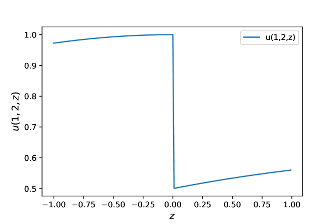
Figure 1: Example 1. The analytic solution (4.6) at $t=1$ and $x=2$ is a discontinuous function of $z$.

Figure 1 shows that the analytic solution (4.6) has a discontinuity at $z=0$ when $x=2$. Figure 2 shows that the expectation and variance of the analytic solution. In this case, one can expect a low convergence rate of the standard gPC-SG method.

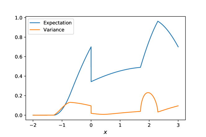
Figure 2: Example 1. The expectation and variance of the analytic solution.

4.1.1 The first order finite difference approximation

In this subsection, we will give the numerical results of our discrete gPC-SG method. Figure 3 shows the numerical expectation and variance compared with the analytic solution with $\Delta x=0.001$, $\Delta t=\dfrac{1}{4}\Delta x$ and gPC order $K=20$. The discrepancy on the variance is due to the poor resolution of the first order spatial discretization, which is improved with the second order spatial discretization to be used later.

Next we conduct the convergence test only for the gPC approximation. We fix $\Delta x=0.005$ and $\Delta t=\dfrac{1}{5}\Delta x$ in all computations with different $K$. Figure 4 shows that the $\ell^{1}$ error decays very fast with respect to the gPC order $K$. When $K=4$, it decays to the numerical error of the finite difference method.

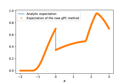
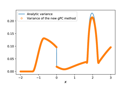
Figure 3: Example 1. The analytic solution compared with the new gPC-SG method using first order finite difference approximation with $\Delta x=0.001$, $\Delta t=\dfrac{1}{4}\Delta x$, gPC order $K=20$.

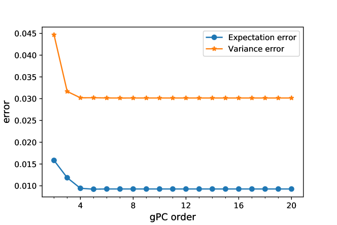
Figure 4: Example 1. The first order finite difference approximation with $\Delta x=0.005$, $\Delta t=\dfrac{1}{5}\Delta x$: the $\ell^{1}$ error versus the gPC order.

However, in Figure 4, since the finite difference error dominates the gPC error, it is difficult to verify the convergence rate of the gPC method. In order to examine the gPC error, we fix $\Delta x$ and $\Delta t$, and compare the numerical solutions with different $K$, with the case of $K=30$ serving as the reference solution. We measure the $\ell^{1}$ error between each $K=2,3,\dotsc,20$ and $K=30$. The result is shown in Figure 5, in which an exponential convergence in the gPC approximation can be observed by using the $\log$-$\log$ plot. Note that if the convergence order is algebraic, the curve should be a line. Here the curve shape shows the exponential decay of the gPC error.

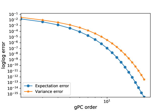
Figure 5: Example 1. The first order finite difference approximation $\Delta x=0.005$, $\Delta t=\dfrac{1}{5}\Delta x$: the gPC error versus the gPC order by a log-log plot (with other numerical parameters fixed).

4.1.2 The second order finite difference approximation

For the second order scheme, we use the same set up as in the first order case. Figure 6 shows the expectation and variance compared with the analytic solution, which gives a more accurate solution than the first order approximation especially for the variance around $x=2$.

Figure 7 and Figure 8 show the convergence of the numerical method in the gPC order from which one can observe the fast convergence. Comparing Figure 7 with Figure 4, we can see that the second scheme has a better total $\ell^{1}$ error. But the rate of the gPC convergence shown in Figure 8 is not as fast as the first order scheme. This is hardly surprising since our spectral convergence depends on the smoothness of the discrete solutions, and the smoothness is given by the numerical viscosity which is larger for the first order spatial discretization. The second order spatial discretization offers better accuracy away from the discontinuities and better resolutions at discontinuities, but because it is closer to the analytic solution (which is not smooth) thus less smooth than the first order one, and smoothness of the discrete solution is what our spectral convergence relies upon, thus its gPC congerence rate, compared with the first order one, should be slower. However this does not mean that the second order method is inferior to the first one, since one has to consider the overall error, including the contributions of error from the spatial discretization in this problem. By comparing Figure 6 with Figure 3, and Figure 7 with Figure 4, it is obvious that the second order scheme outperforms the first order one.

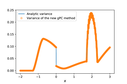
Figure 6: Example 1. The analytic solution compared with the new gPC-SG method using the second order finite difference approximation with $\Delta x=0.001$, $\Delta t=\dfrac{1}{4}\Delta x$, gPC order $K=20$.

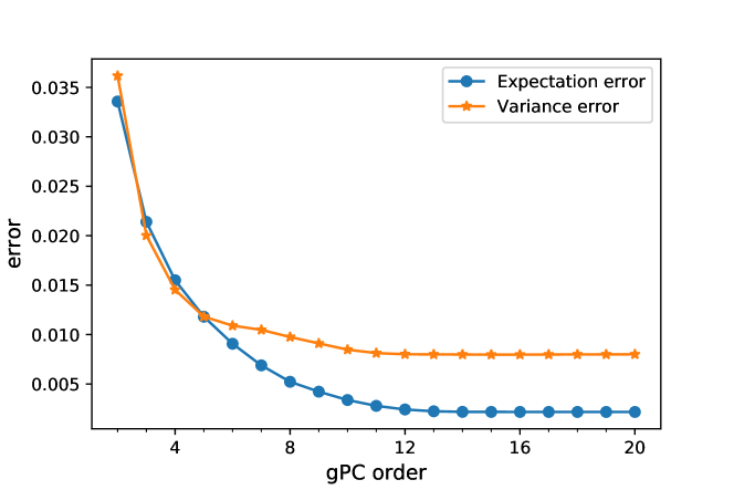
Figure 7: Example 1. The second order finite difference approximation $\Delta x=0.005$, $\Delta t=\dfrac{1}{5}\Delta x$: the $\ell^{1}$ error versus the gPC order.

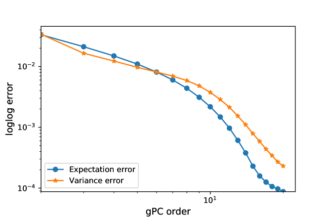
Figure 8: Example 1. The second order finite difference approximation $\Delta x=0.005$, $\Delta t=\dfrac{1}{5}\Delta x$: the gPC error versus the gPC order by a log-log plot (with other numerical parameters fixed).

4.2 Example 2: the Liouville equation with a discontinuous potential

Recall the Liouville equation

$$u_{t}+vu_{x}-V_{x}u_{v}=0,\quad t>0,\quad x,v\in R,$$ (4.7)

with the random potential given by

$$V(x,y)=V_{0}(x)+0.1xz,$$ (4.8)

where $z$ is uniformly distributed on $(-1,1)$ and

$$V_{0}(x)=\begin{cases}0.2,\quad&x<0,\\ 0,\quad&x>0.\end{cases}$$ (4.9)

For the given initial data, one cannot get an analytic solution for this problem. Instead we will use the collocation method as a comparison. In collocation method, one solves the Liouville equation (1.2) at a discrete set of $\{z_{i}\}_{1\leq i\leq M}$ called sample points in the corresponding random space. For every fixed $z_{i}$, we only need to solve a deterministic Liouville equation with discontinuous potential using Hamilton preserving scheme [12]. Then the expectation and variance can be obtained by the quadrature rules of (1.3) and (1.4). In the following examples, we choose $\{z_{i}\}_{1\leq i\leq M}$ as the roots of $M$th order Legendre polynomials and use the Gauss-Legendre quadrature to obtain the expectation and variance.

For the gPC method we need to evaluate $\int_{-1}^{1}V_{0}(z)P_{j}(z)P_{k}(z)\rho(z)\mathop{}\!\mathrm{d}z$, which, for this simple case, is given by

$$\int_{-1}^{1}V_{0}(z)P_{j}(z)P_{k}(z)\rho(z)\mathop{}\!\mathrm{d}z=\begin{cases}\dfrac{j+1}{\sqrt{(2j+1)(2j+3)}},&k=j+1,\\ V^{\prime}_{0}(x),&k=j,\\ \dfrac{j}{\sqrt{4j^{2}-1}},&k=j-1.\end{cases}$$ (4.10)

Here one has a symmetric tridiagonal matrix.

As an illustration of the singularity of the solution caused by the discontinuous potential , we use a continuous initial data:

$$u(x,v,0)=\begin{cases}\sin[2\pi(0.25-(x^{2}+v^{2}))],&x^{2}+v^{2}<0.25,\\ 0,&\text{otherwise}.\end{cases}$$ (4.11)

The expectation of the solution by using the collocation method with $M=20$ sample points and our new gPC-SG method with gPC order $K=4$ are shown in Figure 9.

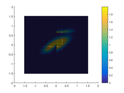
Figure 9: Example 2 with initial data (4.11). Expectation of the solution. Left: the collocation method with $20$ sample points. Right: the new gPC-SG method with gPC order $K=4$.

Although the initial data is continuous, due to the interface condition, the solution may still be discontinuous. This singularity will have a big impact on the convergence of gPC method.

4.2.1 The first order finite difference approximation

In this example we set the initial data as

$$u(x,v,0)=\begin{cases}1,\quad&x\geq 0,v<0,x^{2}+v^{2}<1,\\ 1,\quad&x\leq 0,v>0,x^{2}+v^{2}<1,\\ 0,\quad&\text{otherwise}.\end{cases}$$ (4.12)

Notice that the solution has singularity due to both the initial data and the discontinuous potential. The deterministic version of this example was used in [12] and the analytic solution can be obtained by using the method of characteristics. We first plot the analytic solution and numerical solution (using the first order flux) with a fixed $z=0$ in Figure 10 corresponding to the deterministic example in [12].

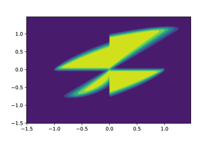
Figure 10: The deterministic case of Example 2 with initial data (4.12). Left: analytic solution of the deterministic problem with $z=0$ and $t=1$. Right: numerical solution using the first order Hamiltonian preserving scheme with $\Delta x=\Delta v=0.015$, $\Delta t=0.001$

Then we compare the solution computed by the collocation method with $M=20$ sample points (Figures 11 and 12 left). Figures 11 and 12 right show the solutions by our new gPC-SG method with gPC order $K=10$. Here the mesh size is $\Delta x=\Delta v=0.03$ and time step is $\Delta t=0.002$. One can see the difference between the expectation of the stochastic solution and the deterministic case when $z=0$ and this differences can be easily seen on the variance plots as well. The expectation of the stochastic solution is expected to be smoother since it integrates over the $z$ variable, thus gains on order of regularity (see examples in [4, 9]). For the computation cost, our new gPC-SG method runs much faster than collocation method. The collocation method takes about $20$ times cost of the deterministic version due to $20$ sample points we choose, however, our new gPC-SG, with $K=10$, takes about $10$ times the cost of the deterministic problem.

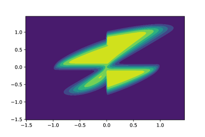
Figure 11: Example 2 with initial data (4.12) by the first order finite difference approximation with $\Delta x=\Delta v=0.03$ and $\Delta t=0.002$. The expectation of the solution. Left: the collocation method with $M=20$ samples points. Right: the new gPC-SG method using first order finite difference approximation.

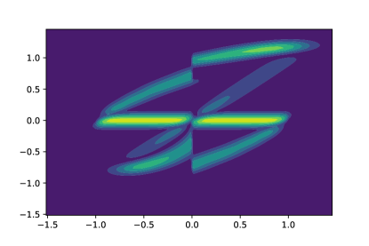
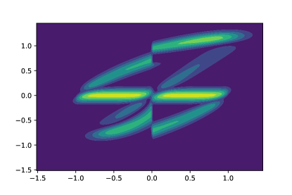
Figure 12: Example 2 with initial data (4.12) by the first order finite difference approximation with $\Delta x=\Delta v=0.03$ and $\Delta t=0.002$. The variance of the solution. Left: the collocation method. Right: the new gPC-SG method.

In Figure 13 we plot the $\ell^{1}$ error of the discrete gPC-SG method as the gPC order $K$ increases. This figure shows the spectral convergence.

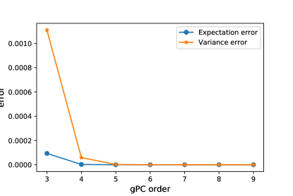
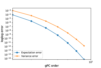
Figure 13: Example 2 with initial data (4.12). Convergence of the new gPC-SG method using the first order finite difference approximation. Left: the $\ell^{1}$ error versus gPC order. Right: the gPC error versus the gPC order by a log-log plot (with other numerical parameters fixed).

4.2.2 The second finite difference approximation

Here for the second finite difference approximation we still use the same set up as in previous subsection for the first order case.

First as in the first order case, we will show the numerical solution of the deterministic case when $z=0$ using the second order flux in Figure 14. The second order method clearly gives a much sharper resolution for the discontinuities than the first order method (compare the right figures of Figure 10 and Figure 15). But due to the Lax-Wendroff scheme we use in the $v$-direction (3.18), there exists some oscillations due to numerical dispersion.

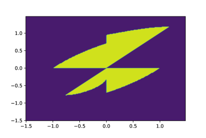
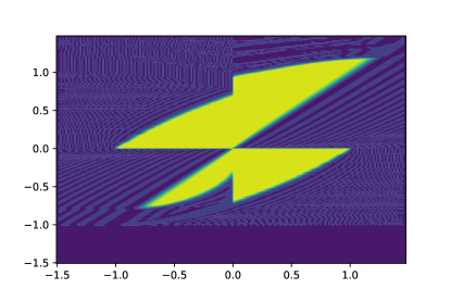
Figure 14: The deterministic case of Example 2 with initial data (4.12). Left: analytic solution of the deterministic problem with $z=0$ and $t=1$. Right: numerical solution using the second order Hamiltonian preserving scheme with $\Delta x=\Delta v=0.015$, $\Delta t=0.001$

Then we will show the expectation and variance of the solution calculated by the collocation method with $M=20$ sample points and our new gPC-SG method (for the calculation of $\left<\mathrm{RHS}(z)\right>$ we also use 20 Gauss-Legendre quadrature points). See Figure 15 and Figure 16.

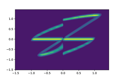
Figure 15: Example 2 with initial data (4.12) by the second order finite difference approximation with $\Delta x=\Delta v=0.03$, $\Delta t=0.002$. Reference solution by the collocation method with 20 sample points at $t=1$. Left: expectation. Right: variance.

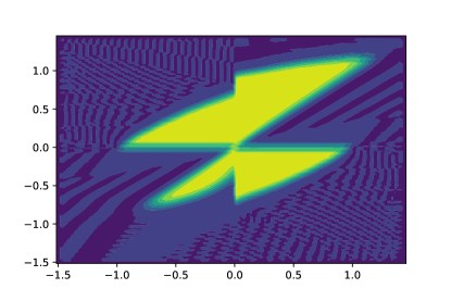
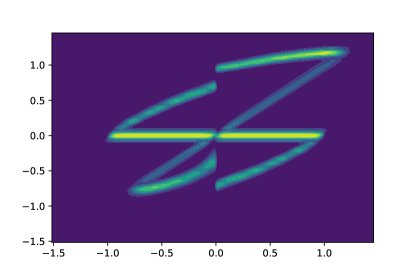
Figure 16: Example 2 with initial data (4.12) by the second order finite difference approximation with $\Delta x=\Delta v=0.03$, $\Delta t=0.002$. Solution at $t=1$ computed by the new gPC-SG method. Left: expectation. Right: variance.

One can find no difference between these two methods, both giving sharper resolutions at discontinuities than their first order counterparts shown in Figures 11 and 12. Here for the computation cost, we point out that unlike in the first order case, our new gPC-SG method runs only slightly faster than the collocation method since in the calculation of $\left<\mathrm{RHS}(z)\right>$ we use a similarly technique as the collocation method.

Finally, we test the convergence rate of our new gPC-SG method. To do this, we first fix our mesh size: $\Delta x=\Delta v=0.03$, $\Delta t=0.02$, and output the result at $t=1$. We use $20$ Gauss-Legendre quadrature points to compute the inner product in (3.20). We choose the gPC order $K=10$ as our reference solution, and see how the error changes when increasing $K$ from $3$ to $10$. From Figure 17, an exponential convergence can be observed.

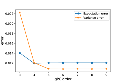
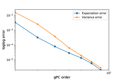
Figure 17: Example 2 with initial data (4.12). Convergence of the new gPC-SG method using second order finite difference approximation. Left: the $\ell^{1}$ error versus the gPC order. Right: the gPC error versus the gPC order by a log-log plot (with other numerical parameters fixed).

References

- [1] H. Bijl, D. Lucor, S. Mishra, C. Schwab, Uncertainty Quantification in Computational Fluid Dynamics, Springer, Cham, 2013. doi:10.1007/978-3-319-00885-1.
- [2] C. Canuto, A. Quarteroni, Approximation results for orthogonal polynomials in Sobolev spaces, Math. Comp. 38 (1982) 67-86. doi:10.1090/S0025-5718-1982-0637287-3.
- [3] H. Choi, J.G. Liu, The reconstruction of upwind fluxes for conservation laws: its behavior in dynamic and steady state calculations, J. Comput. Phys. 144 (1998) 237-256. doi:10.1006/jcph.1998.5970.
- [4] B. Despres, G. Poette, and D. Lucor. Robust uncertainty propagation in systems of conservation laws with the entropy closure method. In Uncertainty Quantication in Computational Fluid Dynamics, Volume 92 of Lect. Notes Comput. Sci. Eng., 105-149. Springer, Heidelberg, 2013
- [5] R. G. Ghanem and P. D. Spanos. Stochastic Finite Elements: A Spectral Approach. Springer Verlag, New York, 1991.
- [6] D. Gottlieb and D. Xiu, Galerkin method for wave equations with uncertain coefficients, Comm. Comp. Phys. 3, 505-518, 2008.
- [7] Max D. Gunzburger, Clayton G. Webster, and Guannan Zhang. Stochastic finite element methods for partial differential equations with random input data. Acta Numer., 23 (2014), 521-650.
- [8] S. Jin, Numerical methods for hyperbolic systems with singular coefficients: well-balanced scheme, Hamiltonian preservation and beyond, Proc. of the 12th International Conference on Hyperbolic Problems: Theory, Numerics, Applications, Univeristy of Maryland, College Park. Proceedings of Symposia in Applied Mathematics Vol 67-1, 93-104, 2009, American Mathematical Society.
- [9] J. Hu, S. Jin, and D. Xiu, A stochastic Galerkin method for Hamilton-Jacobi equations with uncertainty, SIAM J. Sci. Comput. 37, A2246-A2269, 2015.
- [10] S. Jin, K.A. Novak, A Semiclassical Transport Model for Thin Quantum Barriers, Multiscale Model. Simul. 5 (2006) 1063-1086. doi:10.1137/060653214.
- [11] S. Jin, P. Qi, -error estimates on the immersed interface upwind scheme for linear convection equations with piecewise constant coefficients: A simple proof, Science China Mathematics 56 (2013), 2773-2782. doi:10.1007/s11425-013-4738-2.
- [12] S. Jin, X. Wen, Hamiltonian-preserving schemes for the Liouville equation with discontinuous potentials, Commun. Math. Sci. 3 (2005) 285-315.
- [13] S. Jin and X. Wen, Hamiltonian-preserving schemes for the Liouville equation of geometrical optics with partial transmissions and reflections, SIAM J. Num. Anal. 44 (2006), 1801-1828.
- [14] A. Kurganov, E. Tadmor, New High-Resolution Central Schemes for Nonlinear Conservation Laws and Convection Diffusion Equations, J. Comput. Phys. 160, 241-282, (2000). doi:10.1006/jcph.2000.6459.
- [15] O. P. Le Maitre and O. M. Knio. Spectral Methods for Uncertainty Quantification, Scientific Computation, with Applications to Computational Fluid Dynamics. Springer, New York, 2010.
- [16] R.J. LeVeque, Finite Volume Methods for Hyperbolic Problems, Cambridge University Press, 2002.
- [17] M. Motamed, F. Nobile, R. Tempone, A stochastic collocation method for the second order wave equation with a discontinuous random speed, Numer. Math. 123 (2012) 493-536. doi:10.1007/s00211-012-0493-5.
- [18] M. P. Pettersson, G. Iaccarino and J. Nordström, Polynomial Chaos Methods for Hyperbolic Differential Equations, Springer, Switzerland, 2015.
- [19] H. Nessyahu, E. Tadmor, Non-oscillatory central differencing for hyperbolic conservation laws, J. Comput. Phys. (1990).
- [20] T. Tang, T. Zhou, Convergence Analysis for Stochastic Collocation Methods to Scalar Hyperbolic Equations with a Random Wave Speed, Commun. Comput. Phys, 8.1 (2010) 226-248. doi:10.4208/cicp.060109.130110a.
- [21] J. Tryoen, O. Le Maitre, M. Ndjinga, A. Ern, Intrusive Galerkin methods with upwinding for uncertain nonlinear hyperbolic systems, J. Comput. Phys. 229 (2010) 6485-6511. doi:10.1016/j.jcp.2010.05.007.
- [22] D. Xiu, Fast numerical methods for stochastic computations: a review, Comun. Comput. Phys, 5.2-4 (2009) 242-272. doi:10.1016/j.adhoc.2013.06.001.
- [23] D. Xiu, Numerical Methods for Stochastic Computations, Princeton University Press, 2010.
- [24] D. Xiu and G.E. Karniadakis, The Wiener-Askey polynomial chaos for stochastic differential equations. SIAM J. Sci. Comput., 24(2002), 619-644.
- [25] D. Xiu, J.S. Hesthaven, High-Order Collocation Methods for Differential Equations with Random Inputs, SIAM J. Sci. Comput. 27 (2005) 1118-1139. doi:10.1137/040615201.
- [26] T. Zhou, T. Tang, Convergence Analysis for Spectral Approximation to a Scalar Transport Equation with a Random Wave Speed, J. Comput. Math. 30 (2012) 643-656. doi:10.4208/jcm.1206-m4012.