Lagrangian Statistics for Navier-Stokes Turbulence under Fourier-mode reduction: Fractal and Homogeneous Decimations

Abstract

We study small-scale and high-frequency turbulent fluctuations in three-dimensional flows under Fourier-mode reduction. The Navier-Stokes equations are evolved on a restricted set of modes, obtained as a projection on a fractal or homogeneous Fourier set. We find a strong sensitivity (reduction) of the high-frequency variability of the Lagrangian velocity fluctuations on the degree of mode decimation, similarly to what is already reported for Eulerian statistics. This is quantified by a tendency towards a quasi-Gaussian statistics, i.e., to a reduction of intermittency, at all scales and frequencies. This can be attributed to a strong depletion of vortex filaments and of the vortex stretching mechanism. Nevertheless, we found that Eulerian and Lagrangian ensembles are still connected by a dimensional bridge-relation which is independent of the degree of Fourier-mode decimation.

1 Introduction

Turbulence is considered a key fundamental and applied problem [1, 2]. Turbulent flows are distinguished in nature and in the laboratories by the stirring mechanisms and the boundary conditions. Both can be strongly anisotropic, non-homogeneous, and non-stationary, leading to very different realizations for the mean quantities and large-scale velocity configurations. In spite of this large variety, we know that the central feature of all turbulent flows stems from the non-linear terms which are able to transfer to all scales the energy injected by the stirring mechanisms. The non-linear terms are invariant under translation, rotation and mirror symmetries. This is why isotropic, homogeneous and mirror symmetric turbulence is considered a paradigmatic problem for fundamental and applied studies [1].

It is an empirical observation that, in three-dimensional turbulence, energy tends to be transferred from large to small scales intermittently, i.e., producing larger and larger non-Gaussian fluctuations by increasing the Reynolds number (the relative intensity of non-linear versus linear terms in the equations). This is accompanied by the development of anomalous power law scaling for the moments of the velocity increments in the inertial range, i.e., at scales much smaller (larger) than those where the forcing (viscous) term acts. Intermittency of three-dimensional turbulence is not yet fully understood. We cannot connect it to the equation of motion. Neither can we predict its degree of universality, nor the key dynamical and topological ingredients of its origins. For example, two-dimensional turbulent flows are non intermittent with quasi-Gaussian statistics in the inverse cascade regime [3].

In the past, the Navier-Stokes equations (NSE) restricted on a sub-set of Fourier modes have been numerically investigated to gain information about the nature of anomalous scaling, its dependency on the Reynolds number [4, 5, 6], and the effect of local versus non local dynamics on the degree of intermittency see e.g. [7]. More recently, a new decimation protocol has been proposed to ask further questions about the origin of intermittency in the NSE [8, 9]. The idea is again to selectively remove degrees of freedom in the Fourier space, but now implemented in a way to preserve the same conserved quantities and the same symmetries of the original undecimated NSE. By studying the impact of such removal on the flow statistics (in particular, on the intermittent behavior through changing of the projection protocol), a better understanding about the degree of universality and sensitivity of anomalous scaling in turbulence can be achieved.

In this paper, we follow this route further by investigating for the first time the effects of Fourier-mode reduction on the evolution of Lagrangian tracers in turbulence and thus also assessing temporal intermittency. It is well known that Lagrangian particles get strong feedback from the presence of small-scale intense vortex filaments [10, 11, 12]. Studying Lagrangian intermittency under Fourier-mode reduction is therefore a direct way to quantify the robustness of vortex stretching and small-scale vorticity production mechanisms by changing the active degrees of freedom in the dynamical evolution.

We perform a series of direct numerical simulations (DNS) of the three-dimensional NSE by restricting the dynamical evolution on a prescribed quenched set of Fourier modes, and by varying the Reynolds number. We investigate here the case when such a set of modes is a fractal or homogeneous subset of the whole Fourier space. Both these decimation methods belong to the class of spectral tools aiming at solving Navier-Stokes dynamics on a reduced set of wave numbers. The main goals of our theoretical and numerical work are: (i) understanding the impact of mode reduction on the Lagrangian statistics, and (ii) understanding the robustness of Eulerian-Lagrangian bridge relation at changing the scaling properties of the flow.
The effects on the Eulerian statistics induced by the restriction of the dynamics on a fractal set for two- and three-dimensional incompressible turbulence [8, 9, 13, 14], as well as on the one-dimensional Burgers equations [15], have already been reported.

In this paper we extend the previous findings on Eulerian intermittency by considering the case of the homogeneous mode-reduction and by studying its effects on the Lagrangian statistics. We find that homogeneous Fourier-mode decimation is a quasi-singular perturbation for the Lagrangian scaling properties, similar to what is seen for the Eulerian ones. Notwithstanding this fact, we also find that Eulerian and Lagrangian statistics remain strongly correlated, such that the bridge-relation empirically observed for the original undecimated Navier-Stokes equations still holds in the presence of Fourier-mode reduction.

This paper is organized as follows. In Section 2, we introduce the model equations for the Eulerian and Lagrangian dynamics, as well as the decimation protocols; we also define the set-up of the numerical experiments performed, together with the relevant parameters. In section 3 we separately discuss the main results for the velocity field in terms of the Eulerian and Lagrangian statistical properties; while in Section 4 we combine them together by quantitatively assessing the validity of the bridge relation [16, 17, 18, 19, 20, 21]. Summary and discussions are contained in the last section.

2 Model equations for the Eulerian and Lagrangian dynamics

2.1 The decimated equations of motion

Let us define $\bm{u}(\bm{x},t)$ and $\hat{\bm{u}}(\bm{k},t)$ as the real and Fourier space representations of the velocity field, respectively, in dimension $D=3$. We start by considering the Navier-Stokes equations for the incompressible flow with unit density:

$$\partial_{t}{\bm{u}}=-{\bf\nabla}p-(\bm{u}\cdot{\bf\nabla})\bm{u}+\nu\,\nabla^{2}\bm{u}+{\bf F}\,$$ (1)

where $p$ is the pressure and $\nu$ is the kinematic viscosity. ${\bf F}$ is a homogeneous and isotropic forcing which drives the system to a non-equilibrium statistically steady state. Decimation on a generic sub-set of Fourier modes is accomplished by using a generalized Galerkin projector, ${\cal P}$, which acts on the velocity field as follows:

$${\bf v}(\bm{x},t)={\cal P}\,{\bf u}(\bm{x},t)=\sum_{{\bm{k}}}e^{i{\bm{k}\cdot\bm{x}}}\,\gamma_{\bm{k}}\hat{\bm{u}}(\bm{k},t)\,,$$ (2)

where ${\bf v}(\bm{x},t)$ is the representation of the decimated velocity field in the real space. The factors $\gamma_{\bm{k}}$ are chosen to be either 1 or 0 with the following rule:

$$\gamma_{\bm{k}}=\cases{1,&with probability $h_{k}$\\ 0,&with probability $1-h_{k},\,k\equiv|{\bf k}|\,$.}$$ (3)

Once defined, the set of factors $\gamma_{\bm{k}}$ are kept unchanged, quenched in time. Moreover, the factors $\gamma_{\bm{k}}$ preserve Hermitian symmetry $\gamma_{\bm{k}}=\gamma_{-\bm{k}}$ so that ${\cal P}$ is a self-adjoint operator.

The NS equations for the Fourier decimated velocity field are then,

$$\partial_{t}{\bf v}={\cal P}[-{\bf\nabla}p-(\bf v\cdot{\bf\nabla}\bf v)]+\nu\,\nabla^{2}{\bf v}+{\bf F}\,.$$ (4)

We notice that in the above definition of the decimated NSE, the nonlinear term must be projected on the quenched decimated set, to constrain the dynamical evolution to evolve on the same set of Fourier modes at all times. Similarly, the initial condition and the external forcing must have a support on the same decimated set of Fourier modes. In the $(L^{2})$ norm, $\|{\bf v}\|\propto\int|{\bf v}({\bf x})|^{2}d^{3}x$, the self-adjoint operator ${\cal P}$ commutes with the gradient and viscous operators. Since ${\cal P}\,{\bf v}={\bf v}$, it then follows that the inviscid invariants of the dynamics are the same of the original problem in $D=3$, namely energy and helicity.

$N$	$\nu$	$\epsilon$	$\tau_{\eta}$	D $(Re_{\lambda})$	$\alpha$ $(Re_{\lambda})$	$[\%]$
512	0.001	0.79 $\pm$ 0.03	0.035 $\pm$ 0.002	$\frac{3(69);2.99(70);2.98(70);}{2.95(70);2.9(72);2.8(74)}$	——	0; 0.03; 0.06; 0.15; 0.28; 0.46
512	0.001	0.80 $\pm$ 0.01	0.035 $\pm$ 0.001	——	$\frac{0.97(72);0.95(71);0.93(72);}{0.9(73);0.7(72);0.5(82)}$	0.03; 0.05; 0.07; 0.1; 0.3; 0.5
1024	$8\times 10^{-4}$	$1.4\pm 0.2$	$0.023\pm 0.005$	$\frac{3(129);2.99(125);}{2.9(131)}$	—–	0; 0.04; 0.34
1024	$3\times 10^{-4}$	$1.4\pm 0.2$	$0.015\pm 0.003$	2.8 (220)	—–	0.66
1024	$8\times 10^{-4}$	$1.4\pm 0.1$	$0.023\pm 0.003$	——	$\frac{0.99(126);0.95(126);}{0.90(127)}$	0.01; 0.05; 0.1
1024	$3\times 10^{-4}$	$1.3\pm 0.2$	$0.015\pm 0.003$	——	0.60 (205)	0.4

Table 1: Parameters of our direct numerical simulations: $N$ the number of grid points along each spatial direction; $\nu$ the kinematic viscosity; $\epsilon$ the mean energy dissipation rate; $\tau_{\eta}\equiv\sqrt{\nu/\varepsilon}$ the Kolmogorov time scale. The Reynolds number is estimated as $Re_{\lambda}\equiv\sqrt{u_{\rm rms}L/\nu}$, where $u_{\rm rms}$ is the root-mean-square value of the velocity, and $L=2\pi$ is the size of the system; note that at changing the decimation importance, the Reynolds number of the flow can also change, due to an increase of the total kinetic energy in the system (see discussion below). The Reynolds number is given for each run, together with the fractal dimension $D$ or the $\alpha$ values. $D$ is the dimension of the Fourier set for the fractally decimated cases. The values $\alpha$ are the probability used in the cases of homogeneous decimation and $[\%]$ in the last column is the percentage of decimated modes with respect to the non decimated case: it is estimated in the wavenumber range between the mode zero up to the wavenumber where the energy dissipation spectrum peaks.

In this work we adopt two different projectors ${\cal P}$ based on different definitions of the $h_{k}$ factors. One is given by a fractal Fourier decimation, first introduced in [8] as:

$$h_{k}\propto(k/k_{0})^{D-3}\,,\quad\quad\mbox{with}\quad\quad 0<D\leq 3\,,$$

where $k_{0}$ is a small wavenumber here always taken to be 1. This decimation ensures that the dynamics is restricted isotropically to a $D$-dimensional Fourier sub-space. Note that this implies that the velocity field is embedded in a three-dimensional space, but effectively possesses a set of degrees of freedom (DOF) inside a sphere of radius $k$ growing as $\#_{DOF}(k)\sim k^{D}$. The smaller the fractal dimension $D$, the slower is the associated growth of the DOF. Moreover, the decimation clearly has a larger impact towards the ultra-violet cutoff, since modes in the high wave number range have a larger probability to be decimated. Note that this is different from studying NSE in geometries with one compactified dimension, as previously reported [22].

The second choice consists of keeping the degree of mode reduction homogeneous in the wave number range:

$$h_{k}=\alpha,\quad\forall k;\qquad\mbox{with}\qquad 0\leq\alpha\leq 1\,.$$

2.2 Set-up of the numerical experiments

We performed different series of direct numerical simulations of the incompressible Navier-Stokes equations in a 2$\pi$-periodic volume, with a standard pseudo-spectral approach fully dealiased with the two-thirds rule. Time stepping is done with a second-order Adams-Bashforth scheme.

The first set of simulations is done by using $N^{3}=512^{3}$ collocation points. In these runs, a constant energy injection forcing [23, 24] acting only at large scales, $1\leq k_{\rm force}\leq 2$, is implemented to keep the system in a statistically steady state. The second set of simulations is done with $N^{3}=1024^{3}$ grid points. A statistically steady, homogeneous and isotropic turbulent state is maintained by forcing the large scales, $0.5\leq k_{\rm force}\leq 1.5$, of the flow via a second-order Ornstein-Uhlenbeck process [25]. The choice to adopt a time-correlated process for the forcing is dictated by the requirement to enforce the continuity of the acceleration of particles. In all simulations with $N=1024$, the correlation time-scale of the forcing is $\sim 10\tau_{\eta}$ so that small scales are unaffected by the precise forcing mechanism. For both resolutions, we perform different sets of DNS for different values of the fractal dimension $D$ or the decimation percentage $\alpha$. In our study, we define the Reynolds number as $Re_{\lambda}\equiv\sqrt{u_{\rm rms}L/\nu}$, where $u_{\rm rms}$ is the root-mean-square value of the velocity field and $L=2\pi$ is the size of the system. In Table  1, for each run we report the fractal dimension $D$ or the $\alpha$ values, together with the estimated Reynolds number.

To obtain the Lagrangian statistics, we seeded the flow with tracer particles. The particles do not react on the flow and do not interact amongst themselves. The trajectories of individual particles are described via the equation:

$$\frac{\mathrm{d}{\bm{X}}}{\mathrm{d}{t}}={\bf v}(\bm{X}(t),t)\,,$$

and are integrated by using a trilinear or B-spline 6th order interpolation scheme  [26], to obtain the fluid velocity, ${\bf v}(\bm{X}(t),t)$, at the particle position. We note that Galerkin truncation or decimation operators destroy the Lagrangian structure of the NS dynamics. However, it is clear that studying the Lagrangian dynamics in turbulent decimated flows is always possible, and, as we will see, it is an important piece of information when dealing with the nature of intermittency in hydrodynamical turbulence.

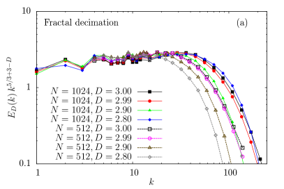
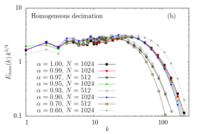
Figure 1: Compensated kinetic energy spectra (a) $k^{5/3+D-3}E(k)$ for fractal and (b) $k^{5/3}E(k)$ for homogeneous decimation. The spectra have been shifted to obtain a collapse onto a single curve, for ease in visualization.

3 Results

3.1 Spectra

As shown in [9], fractal decimation induces a correction, $\propto k^{3-D}$, for the power law scaling of the kinetic energy spectrum:

$$E_{D}(k)\sim k^{3-D}\,k^{-5/3}\,,$$ (5)

where the factor $\sim k^{-5/3}$ is the K41 spectrum predicted by Kolmogorov in $1941$ theory and valid for the $D=3$ original problem (we neglect intermittent corrections). The derivation of this result can be found in [9]: it is based on the empirical observation that the energy flux, $\epsilon$, remains constant in the inertial range of scales and for all fractal dimensions. In order to keep a constant flux across all scales, with less and less modes, the spectrum must acquire a power-law correction. Note that the extra power-law correction induced by the fractal decimation introduces new contributions in the Eulerian domain, leading to a complex superposition of scaling properties as shown in [9, 14, 15]. Furthermore, this makes it even more difficult to interpret Lagrangian statistics starting from the Eulerian phenomenology.
Since for the homogeneous case the decimation probability is constant and independent of $k$, these difficulties are absent and we expect a K41 spectra for all $\alpha$:

$$E_{hom}(k)\sim k^{-5/3}.$$ (6)

In Fig. 1 we confirm the two predictions (5)-(6) by showing the compensated energy spectra for the case of (a) fractal ($E_{D}(k)k^{D-3+5/3}$) and (b) homogeneous ($E_{hom}(k)k^{5/3}$)decimations. The curves all collapse for all the values of $D$ and $\alpha$.
Before concluding this section, we comment that the power-law correction of the spectrum exponent for the fractal cases is such that for $D=7/3$, the spectrum becomes divergent in the region of large $k$. Numerically, the investigation of the system at such low fractal dimension is critical, since e.g. at resolution $N=1024$ about less than 1% of the modes would survive. The actual behavior of the system at dimensions close to $7/3$ remains an open question.

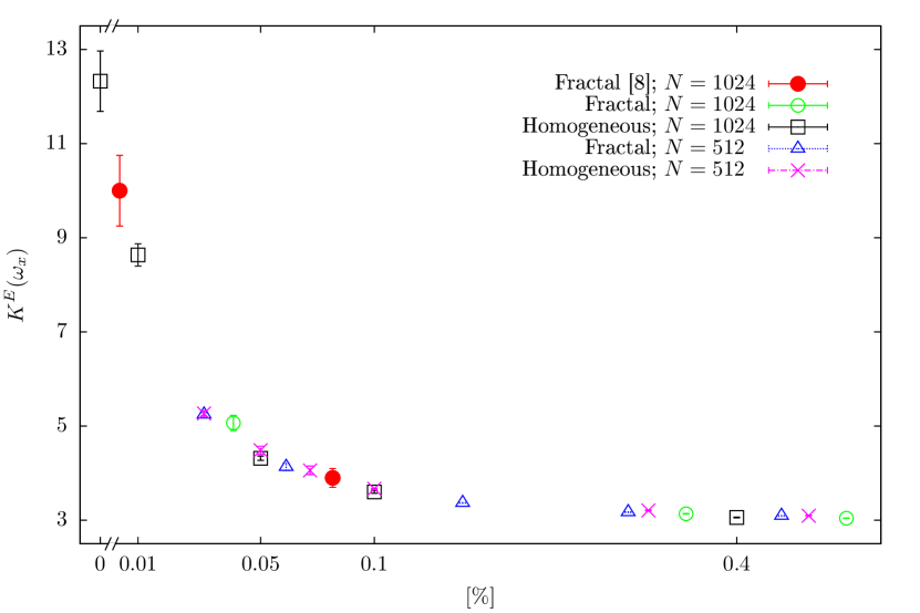
Figure 2: The kurtosis of the x-component of the vorticity field $K^{E}(w_{x})$ vs the percentage of decimated Fourier modes, $[\%]$. The explicit values of the percentage of decimation and the corresponding fractal dimension $D$ or the probability of homogeneous decimation $\alpha$ are listed in Table 1.

3.2 Higher-Order Eulerian Statistics

In three-dimensional turbulence, the distribution of the spatial derivatives of the velocity field has a strongly non-Gaussian behavior. A measure of this is given by the kurtosis of one component of the vorticity field (assuming small-scales isotropy):

$$K^{E}(w_{x})=\frac{\langle\omega_{x}^{4}\rangle}{\langle\omega_{x}^{2}\rangle^{2}}\,\,.$$

A Gaussian distribution is characterized by $K^{E}=3$. It is known that in three-dimensional turbulence, the kurtosis is larger than 3 and grows as a function of the Reynolds number, indicating that the flow is becoming more and more intermittent. It was previously observed [9, 14] that when fractal decimation is applied, the kurtosis approaches the Gaussian value with decreasing $D$. In Figure 2 we show the value of the kurtosis $K^{E}(w_{x})$ as a function of the percentage of removed modes $[\%]$ (defined below and listed in Table 1) for both fractal and homogeneous decimations as well as for the different Reynolds numbers. To make the comparison between the fractal and homogeneous protocols meaningful, we use the percentage of mode reduction in the fractal case measured as the percentage of modes removed up to $k_{\rm peak}$, i.e., up to the wavenumber where the dissipation energy spectrum $k^{2}E_{D}(k)$ peaks. For homogeneous decimation, the percentage of removed modes $[\%]$ is simply $1-\alpha$. Our results show that not only does the homogeneous decimation cause a suppression of intermittency, but the effect takes place with the same dependence on the percentage of removed modes as measured in the fractal case. Moreover, we see that our data from these sets of simulations are in agreement with data from [9] where a different forcing was used. To summarize, turbulent decimated systems show a unique tendency towards a quasi-Gaussian statistics, independent of the decimation protocol.

The suppression of spatial intermittency under decimation leads us to the main question of this paper: what happens to the Lagrangian dynamics when small-scale structures responsible for the vortex stretching are largely modified [14], if not destroyed? To answer this question we stick to the homogeneous decimation case in order to avoid the further complication induced by the power-law correction present in the velocity scaling in the fractal case.

3.3 Lagrangian Statistics

In this section, we analyze the statistical behavior of tracer particles in decimated flows. In order to do that it is useful to define the order-$p$ Lagrangian structure function:

$$S^{L}_{p}(\tau)\equiv\sum_{i}\,\langle[\delta_{\tau}v_{i}]^{p}\rangle\sim\,\tau^{\zeta_{p}^{L}}\,,$$ (7)

where $\delta_{\tau}v_{i}=v_{i}(\bm{X}(t+\tau),t+\tau)-v_{i}(\bm{X}(t),t)$ and the sum is over the three components of the velocity field (assuming isotropy). As for the Eulerian case, we quantify deviations from Gaussian statistics at changing time lags by defining the Lagrangian kurtosis:

$$K^{L}(\tau)=\frac{S^{L}_{4}(\tau)}{(S^{L}_{2}(\tau))^{2}}.$$ (8)

$K^{L}(\tau)$ evaluated at time increment $\tau=\tau_{\eta}$ is plotted in Fig. 3. It shows a strong dependence on the number of DOF, similar to what happens for the Eulerian case. The dependence on the Reynolds number of the flow is weak as we find that the measurements done in the DNS with $N=512$ or $N=1024$ exhibit the same behavior. Notice that in Figure  3, the value of the kurtosis for the smallest time scale is very close to the one obtained by looking at the acceleration of the particles.

To quantify the Lagrangian properties at all time lags $\tau$, we show in the inset of the same figure the kurtosis of tracers for all $\tau$. It is clear that there is a rapid reduction of intermittency, as it was reported in [9], just like the corresponding Eulerian measurements made for spatial increments. Since Lagrangian statistics are known to be more intermittent than their Eulerian counterparts (as quantified by the deviations from the dimensional scaling), this result is even more interesting. This is because it shows how a nominally small decimation ($\alpha=0.95$) is responsible for a decrease of about $85\%$ of the kurtosis at small $\tau$. We attribute such a large reduction to the strong modification of intense vortical structures as reported in a previous study [14]. Moreover, the quick recovery of quasi-Gaussian statistics by increasing the degree of decimation is, for this observable and for the Reynolds numbers investigated here, almost independent of the Reynolds number. It is also noteworthy that the results are independent of the particular type of large-scale forcing since the form of forcing for $N=512$ differs from the case of $N=1024$.

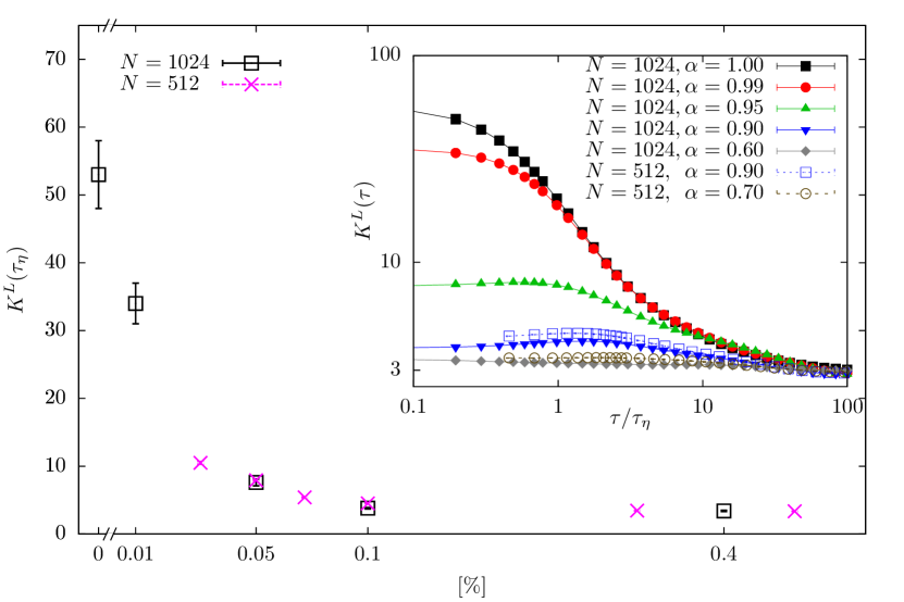
Figure 3: The kurtosis $K^{L}(\tau)$ of the Lagrangian structure function measured at the Kolmogorov time scale $\tau=\tau_{\eta}$ as a function of the percentage of decimated Fourier modes $[\%]$. In the inset we show representative plots of $K^{L}(\tau)$ vs $\tau$ for some values of $\alpha$

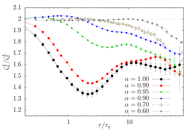
Figure 4: Log-lin plot of the local slopes of the scaling exponent $\zeta_{4}^{L}/\zeta_{2}^{L}$ of the Lagrangian structure functions, averaged over the three velocity components, vs $\tau/\tau_{\eta}$ for some representative value of $\alpha$ from the simulations at $N=1024$.

To have a deeper understanding of the Lagrangian scaling, in Figure 4, we plot the local slopes by using Extended Self Similarity (ESS) [19, 27, 28], i.e., the logarithmic derivative of the fourth order Lagrangian structure function, $S^{(4)}_{L}(\tau)$, versus the second order one, $S^{(2)}_{L}(\tau)$, which gives:

$$\frac{d\log S^{L}_{4}(\tau)}{d\log S^{L}_{2}(\tau)}=\frac{\zeta^{L}_{4}}{\zeta^{L}_{2}}\,.$$ (9)

Let us notice that the above quantity is a direct scale-by-scale measurement of the local scaling properties and does not need any fitting procedure. A scale-independent behavior of one moment against the second-order one would result in a constant value for the left hand side of (9). We recall that in the absence of intermittency, these curves should be constant across the time lags with $\zeta^{L}_{4}/\zeta^{L}_{2}=2$; while this relation is always well verified for the smooth dissipative scales, a non trivial behavior appears in the inertial range pointing out the intermittent feature of the original system. A few important observations should be made. First, in the time range from $1$ to $10\,\tau_{\eta}$, the strong deviation observed in the local slope of the standard $D=3$ case and attributed to events of tracer trapping in intense vortex filaments [29] rapidly disappears as soon as the mode reduction is applied. Second, we observe that in the inertial range (where the $D=3$ local exponents develop a plateaux) the scaling for the decimated cases is much poorer, i.e. the local-slopes are no longer constant. Finally, independent of the existence of a pure scaling behavior, we observe that the intermittent correction is also reduced as the percentage of removed modes is increases, and it almost vanishes, reaching the dimensional value $2$ for almost all $\tau$, already at $\alpha=0.6$, corresponding to $40\%$ of the modes decimated. These observations are valid for all the Reynolds numbers here explored.

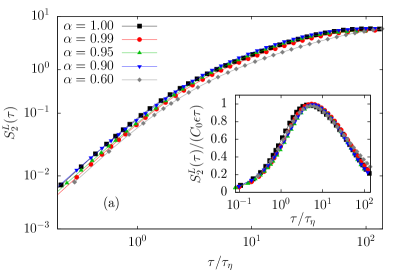
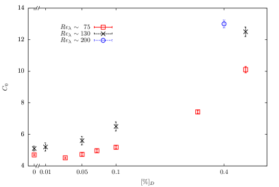
Figure 5: (a) Log-log plot of the second-order Lagrangian structure function $S^{L}_{2}(\tau)$ vs $\tau/\tau_{\eta}$, averaged over the three velocity components, for some representative values of $\alpha$. In the inset we show the linearly compensated second-order Lagrangian structure function, $S^{L}_{2}(\tau)/(C_{0}\,\epsilon\tau)$; the dimensionless constant $C_{0}$ is chosen such that the peak of the compensated structure function is 1. In (b) we show the variation of $C_{0}$ as a function of $[\%]$ for the homogeneously decimated cases, and for runs at comparable Reynolds numbers: the upper curve is for $Re_{\lambda}\simeq 130$ ($\times$), while the lower curve is for $Re_{\lambda}\simeq 75$ (squares). The isolated circle point is for the numerical simulation at $N=1024$, viscosity $nu=3.e-4$ and $\alpha=0.6$, for which the estmated Reynolds number is higher than the other cases.

4 Connecting Eulerian and Lagrangian Statistics in Decimated Flows

An important open point in literature is connected to the relation between Eulerian and Lagrangian statistics [16, 19, 21, 30, 31, 32, 33, 34]. The two ensembles must of course be correlated. Let us introduce the order-$p$ Eulerian structure function in a manner analogous to the definition of the Lagrangian structure function. For the longitudinal velocity increments $\delta_{r}v=[{\bf v}({\bf x}+{\bf r})-{\bf v}({\bf x})]\cdot{\hat{r}}$, the longitudinal Eulerian structure function can be written as

$$S^{E}_{p}(r)\equiv\langle[\delta_{r}v]^{p}\rangle\sim r^{\zeta^{E}_{p}}.$$ (10)

Similarly, one could have introduced transverse Eulerian structure functions, based on transverse increments [1]. Dimensional predictions based on the idea that in the inertial range everything is driven by the energy transfer rate, $\epsilon$, puts strong constraints on the possible functional dependencies of Eulerian and Lagrangian structure functions. For example, dimensional predictions give $\zeta_{p}^{E}=p/3$ and $\zeta_{p}^{L}=p/2$. It is also known that in the presence of intermittent corrections, where $\zeta_{p}^{E}\neq p/3$ and $\zeta_{p}^{L}\neq p/2$, the two sets of exponents are well explained by a bridge relation [16, 17, 18, 21]. The idea is to connect the spatial and temporal fluctuations over increment $r$ and $\tau$ by

$$\delta_{\tau}v\sim\delta_{r}v;\qquad\qquad\tau\sim r/\delta_{r}v\,.$$ (11)

Applying the usual multifractal formalism, is then possible to show that the following relation holds [16, 17, 18, 21]:

$$\zeta^{L}_{p}=\zeta^{E}_{n}\,,$$ (12)

$$p\,=n\,-\zeta^{E}_{n}\,.$$ (13)

It is important to notice that the above relation is consistent with the dimensional phenomenology. Moreover, considering that we have the exact Eulerian result $\zeta_{3}^{E}=1$, the second order Lagrangian structure function must scale linearly according to (13), $\zeta_{L}^{2}=1$:

$$S^{L}_{2}(\tau)=C_{0}\epsilon\tau\,.$$ (14)

Different scaling properties for three-dimensional Lagrangian turbulence have also been proposed, as discussed in [33]. The question of whether this bridge relation is exact or a very good first-order approximation is still open. Since, even under decimation, one can prove that $\zeta_{3}^{E}=1$, it is important to check whether the above prediction (14) still holds (empirically) under the application of homogeneous decimation. In Figure 5(a), we plot the second order moment of velocity increments, averaged over the three field components, for the homogeneously decimated runs at $N=1024$. We note that all curves exhibit a similar behavior, which also means that there is no evident difference between data of $D=3$ standard turbulence, and the data from the decimated cases, in agreement with (14).

In the inset of the same figure we also plot the compensated curves, $S_{2}^{E}(\tau)/(C_{0}\epsilon\tau)$ versus $\tau$. Looking at the compensated plots, we can observe better the agreement among $D=3$ and decimated turbulence. Such a good overlap of the different curves is obtained by accurately fixing the values of two parameters. First, the Kolmogorov time scale $\tau_{\eta}$ is varied within the error bars given in Table 1 to obtain an optimal horizontal shift. Second, the coefficient $C_{0}$ is also changed in order to fix the peak of the correlation at $1$. The value of normalization constant $C_{0}$ has been already examined in previous works and it is known to depend on the Reynolds number of the flow, see e.g. [35, 36]. For high Reynolds numbers in three-dimensional turbulence, it is estimated that $C_{0}$ lies in the range $6-7$. In our simulations, we have measured for $D=3$ the value $C_{0}=5.2$ for $N=1024$, which is in agreement with the previous measurements at the same Reynolds number. The measured behavior of $C_{0}$ as a function of the percentage of removed modes $[\%]$ is interesting. In panel (b) of Figure 5, we see that it grows as the reduction of the DOF in the system increases. This result is in agreement with the observation first reported in [8] that, at increasing decimation, a less efficient energy transfer towards small-scale leads to a growth of total kinetic energy due to an accumulation at the largest scales of the system. We also note that for any given value of the percentage of modes decimated, $C_{0}$ is slightly larger for the homogeneous runs with higher Reynolds number. We remark that $C_{0}$ is known to be strongly sensitive to the underlying Eulerian flow realization, since for example in two-dimensional (undecimated) turbulence in the inverse cascade regime [20], it can become as large as 40-50 depending on the inertial range extension.
The scaling properties of $S^{L}_{2}(\tau)$ show that the bridge relation is robust under mode reduction, at least for those observables that are not affected by intermittency. We now ask the same question for higher order moments, where intermittency play a major role and strongly depends on the degree of mode reduction. In Figure 6, we test on the numerical data the bridge-relation (13) for the Lagrangian scaling exponent $\zeta^{L}_{4}/\zeta^{L}_{2}$. To do this, we first need to estimate from the Eulerian data a functional form for the curve of the scaling exponents, $\zeta^{E}_{p}$ of the structure functions for different values of $p$. We accomplish this by repeating the procedure illustrated e.g. in [19], by using the multifractal model and a log-Poisson distribution for the singularity spectrum. Details are not repeated here for the sake of brevity.
The shaded area around each curve represents our uncertainty on the local Lagrangian scaling exponents, based on the Eulerian ones: indeed in the Eulerian framework, scaling exponents are not defined uniquely since longitudinal and transverse moments are observed to scale differently, see e.g., [37]. The shaded area is associated to the different sets of Lagrangian scaling exponents that we can obtain considering either the longitudinal or the transverse moments scaling in the Eulerian framework, and hence in the relations (12) and (13). The agreement is remarkable.

To summarize, we have tested, a non-linear set of relations bridging Eulerian scaling exponents to Lagrangian ones. These transformations are based on the idea that statistical relations among velocity singular fluctuations do survive decimation protocols, and can then be used even when the detailed form of the Navier-Stokes equations is modified by a strong reduction of the degrees of freedom.

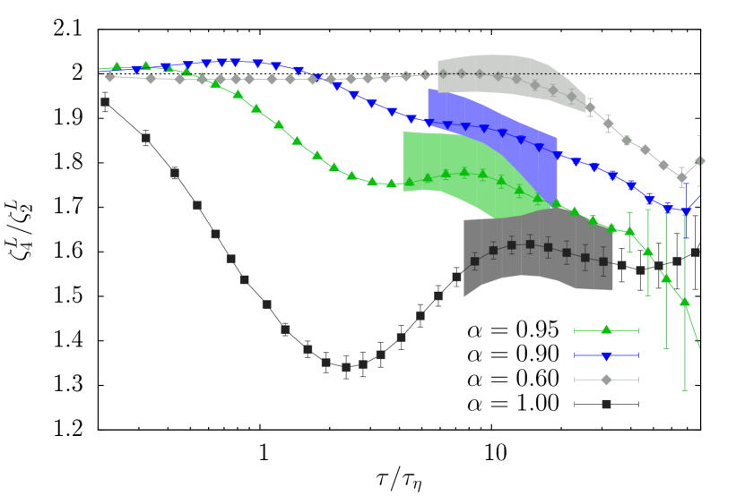
Figure 6: Log-lin plot of the local slopes of the scaling exponent $\zeta_{4}^{L}/\zeta_{2}^{L}$ of the Lagrangian structure functions, averaged over the three velocity components, vs the time lag $\tau/\tau_{\eta},$ for some representative values of $\alpha$ from simulations with higher Reynolds number. The shaded region shows the inertial range prediction from the multifractal model by using the Eulerian longitudinal and transversal structure functions. The straight dashed line correspond to the dimensional non-intermittent value $\zeta_{4}^{L}=2\zeta_{L}^{2}$. The overlap of the shaded regions with the corresponding data from our numerical simulations is a confirmation of the validity of the bridge relations (see text), connecting the Eulerian and Lagrangian scaling exponents.

5 Conclusions

We have performed a series of direct numerical simulations of the three-dimensional NSE under Fourier mode reduction. Projection on a restricted set of Fourier modes has been largely explored in the past, starting from the pioneering work of Lee and Hopf to study the Euler equations with the tools of equilibrium statistical mechanics [38, 39, 40, 41] or to search for flux-less solutions with scaling properties close to the Kolmogorov $-5/3$ spectrum in the inverse cascade regime [8, 42]. Here, we have shown that Fourier mode reduction also offers a unique opportunity to change the degree of intermittency of the NSE and thus to study its robustness under a wide spectrum of different perturbations. Fourier mode reduction has a singular effect on the dynamics: a weak removal of modes strongly modifies the scaling properties of turbulent flows.

In this study, we have applied to the original three-dimensional problem two decimation protocols, where the degree of mode reduction is changed continuously through different control parameters. In both cases the resulting dynamics preserves the inviscid conservation properties and all symmetries of the original problem. Fractal decimation constraints the set of Fourier modes to live on a fractal set, with the high-wavenumber degrees of freedom having a larger probability to be decimated, leading to a larger and larger weight of non-local Fourier interactions by decreasing $D$. Moreover, fractal decimation modifies the scaling exponent of the kinetic energy spectrum, thus introducing a complex superposition of scaling behaviors in the Eulerian domain. Homogeneous decimation removes degrees of freedom with the same percentage from large to small scales, without introducing new scaling properties and keeping the same statistical weight of local and non-local triadic interactions in the non-linear evolution. We have first shown that both protocols reduce intermittency with the same dependence on the number of DOF in the system in the Eulerian frame, and at the two Reynolds numbers here investigated. Some runs have also been repeated by keeping all parameters unchanged, expect for the stochastic realization of the decimation mask to check that the statistical measures that we report are indeed independent of the precise quenched realization of the DOF reduction.

Concerning the Lagrangian statistics, we have shown that homogeneous decimation leads to a quick reduction of high-frequency intermittency too, as measured by the kurtosis of the Lagrangian structure functions at the Kolmogorov time scale. This reduction of intermittency is accompanied by a quick increase of the $C_{0}$ constant in the second order Lagrangian structure function, indicating a possible singular behavior in the high decimated regime at large Reynolds numbers. It is important to recognise that in the limit of infinite Reynolds number, the fractal and homogeneous decimation protocols will probably lead to very different asymptotics. This is because, as the Reynolds number increases, smaller and smaller scales appear which will be decimated with a larger and larger probability for the fractal decimation protocol or with a constant probability for the homogeneous case.

Interestingly, in spite of the strong sensitivity of intermittency on the degree of mode reduction, the two sets of Lagrangian and Eulerian structure functions remain well-described by a phenomenological bridge-relation, which connects the degrees of intermittency in the two set of measurements. Besides the previous findings, the outcome of the present work can be seen as an attempt to characterize the statistical properties of the NSE when restricted to a reduced set of modes and before applying a sub-grid closure for the removed DOF. This Large-Eddy-Simulation program is typically implemented by applying a sharp cutoff at $k_{c}$ in Fourier space for all wavenumbers with $k>k_{c}$. Here, the cutoff is still sharp (we apply a projector) but the grid is diffused among the whole Fourier space, keeping memory of all scales and frequencies in the system. This might be crucial to further improve the modelling of the evolution of particles in turbulent flows. In particular, the impact of fractal or homogeneous mode reductions on the Lagrangian and Eulerian statistics can be seen as a first step toward the development of models for the removed degrees-of-freedom, which is the ultimate goal of any Large-Eddy-Simulation. The strong sensitivity of intermittency to the degree of mode reduction is a clear indication that this is a delicate issue that needs to be investigated with care.

References

References

- [1] U. Frisch, Turbulence: The Legacy of A.N. lmogorov (Cambridge University Press, Cambridge, United Kingdom, 1996).
- [2] S. B. Pope, Turbulent Flows (Cambridge University Press, 2000).
- [3] G. Boffetta, A. Celani, and M. Vergassola, Phys. Rev. E 61, R29 (2000).
- [4] S. Grossmann, D. Lohse, and A. Reeh, Phys. Rev. Lett. 77, 5369 (1996).
- [5] M. Meneguzzi, H. Politano, A. Pouquet, and M. Zolver, J. Comput. Phys. 123, 32 (1996).
- [6] F. De Lillo and B. Eckhardt, Phys. Rev. E 76, 016301 (2007).
- [7] J.-P. Laval, B. Dubrulle, and S. Nazarenko, Phys. Fluids 13, 1995 (2001).
- [8] U. Frisch, A. Pomyalov, I. Procaccia, and S. S. Ray, Phys. Rev. Lett. 108, 074501, (2012).
- [9] A. S. Lanotte, R. Benzi, S. K. Malapaka, F. Toschi, and L. Biferale, Phys. Rev. Lett. 115, 264502 (2015).
- [10] A. La Porta, G. A. Voth, A. M. Crawford, J. Alexander, and E. Bodenschatz, Nature (London) 409, 1017 (2001).
- [11] L. Biferale, G. Boffetta, A. Celani, A. Lanotte, and F. Toschi, Phys. Fluids 17, 021701 (2005).
- [12] A. Pumir, H. Xu, E. Bodenschatz, and R. Grauer, Phys. Rev. Lett. 116, 124502 (2016).
- [13] S. S. Ray, Persp. Nonlin. Dyn., PRAMANA- J. Phys., 84, 395, (2015).
- [14] A.S. Lanotte, S. K. Malapaka, and L. Biferale, Eur. Phys. J. E 39, 49 (2016).
- [15] M. Buzzicotti, L. Biferale, U. Frisch, and S. S. Ray, Phys. Rev. E 93, 033109 (2016).
- [16] M.S. Borgas, Phil. Trans. R. Soc. London A 342 379 (1993).
- [17] L. Biferale, G. Boffetta, A. Celani, B.J. Devenish, A.S. Lanotte, and F. Toschi, Phys. Rev. Lett. 93, 064502 (2004).
- [18] F. G. Schmitt, Phys. A 368, 377–386 (2006).
- [19] A. Arnéodo et al., Phys. Rev. Lett. 100, 254504 (2008).
- [20] A.S. Lanotte, L. Biferale, G. Boffetta, and F. Toschi, J. Turb. 14(7), 34–48 (2013).
- [21] G. Boffetta, F. De Lillo, and S. Musacchio, Phys. Rev. E 66, 066307 (2002).
- [22] A. Celani, S. Musacchio and D. Vincenzi, Phys. Rev. Lett 104, 184506 (2010).
- [23] A.G. Lamorgese, D.A. Caughey, and S.B. Pope, Phys. Fluids 17, 015106 (2005).
- [24] G. Sahoo, P. Perlekar, and R. Pandit, New J. Phys. 13, 0130363 (2011).
- [25] B. L. Sawford, Phys. Fluids A 3, 1577 (1991).
- [26] W. H. Press, Numerical Recipes 3rd Edition: The Art of Scientific Computing (Cambridge University Press, Cambridge, United Kingdom, 2007).
- [27] R. Benzi, S. Ciliberto, C. Baudet, F. Massaioli and S. Succi, Phys. Rev. E 48, R29 (1993).
- [28] S. Chakraborty, U. Frisch and S. S. Ray, J. Fluid Mech. 649, 275 (2010).
- [29] L. Biferale, G. Boffetta, A. Celani, A.S. Lanotte, and F. Toschi, Phys. Fluids 17, 021701 (2005).
- [30] L. Chevillard, S.G. Roux, E. Leveque, N. Mordant, J.-F. Pinton, and A. Arnéodo, Phys. Rev. Lett., 91, 214502 (2003).
- [31] R, Benzi L. Biferale, R. Fisher, D.Q. Lamb and F. Toschi Journ. Fluid Mech. 653, 221, (2010).
- [32] H. Homann, O. Kamps, R. Friedrich, and R. Grauer, New J. Phys. 11, 073020 (2009).
- [33] G. Falkovich, H. Xu, A. Pumir, E. Bodenshatz, L. Biferale, G. Boffetta, A.S. Lanotte, and F. Toschi, Phys. Fluids 24, 055102 (2012).
- [34] E. Leveque and A. Naso, Europhys. Lett. 108 54004 (2014).
- [35] P. K. Yeung, Annu. Rev. Fluid Mech. 34, 115–142 (2002).
- [36] B.L. Sawford and P.K. Yeung, Phys. Fluids 23 091704 (2011).
- [37] L. Biferale, A. S. Lanotte, and F. Toschi, Phys. D 237, 1969–1975 (2008).
- [38] R. H. Kraichnan, Adv. Math. 16, 305–331 (1975).
- [39] C. Cichowlas, P. Bonaïti, F. Debbash, and M.-E. Brachet, Phys. Rev. Lett. 95, 264502 (2005).
- [40] U. Frisch U, S. Kurien, R. Pandit, W. Pauls, S.S. Ray, A. Wirth, and J.Z. Zhu, Phys Rev Lett. 101, 144501 (2008).
- [41] S. S. Ray, U. Frisch, S. Nazarenko, and T. Matsumoto, Phys. Rev. E 84, 016301, (2011).
- [42] V. L’vov, A. Pomyalov, and I. Procaccia, Phys. Rev. Lett. 89, 064501 (2002).