Diósi-Penrose criterion for solids in quantum superpositions and a single-photon detector

Garrelt Quandt-Wiese

Schlesierstr. 16, 64297 Darmstadt, Germany
garrelt@quandt-wiese.de
  http://www.quandt-wiese.de

A formulary for the application of the Diósi-Penrose criterion to solids in quantum superpositions is developed, which takes the solid’s microscopic mass distribution (resulting from its nuclei) and its macroscopic shape into account, where the solid’s states can differ by slightly different positions or extensions of the solid. For small displacements, smaller than the spatial variation of the solid’s nuclei, the characteristic energy of the Diósi-Penrose criterion is mainly determined by the mass distribution of the nuclei. For large displacements, much larger than the solid’s lattice constant, the solid can be idealised as a continuum, and the characteristic energy depends on the solid’s shape and the direction of the displacement. In Diósi’s approach, in which the mass density operator has to be smeared, the solid’s microscopic mass distribution plays no role. The results are applied to a special single-photon avalanche photodiode detector, which interacts as little as possible with its environment. This is realised by disconnecting the detector from the measurement devices when it is in a superposition, and by biasing the photodiode by a plate capacitor, which is charged shortly before the photon’s arrival. For a suitable choice of components, the detector can stay in a superposition for seconds; its lifetime can be shortened to microseconds with the help of a piezoactuator, which displaces a mass in the case of photon detection.

1 Introduction

The Diósi-Penrose criterion is a rule of thumb for estimating the lifetimes of quantum superpositions. The lifetime of a superposition scales with the inverse of a characteristic gravitational energy, which only depends on the mass distributions of the superposed states [1, 5, 6]. The Diósi-Penrose criterion is often used for quantitative assessments of experimental proposals aiming to measure some aspects of wavefunction collapse [7, 8, 9, 10, 11, 12, 13, 14]. It arises from gravity-based approaches to wavefunction collapse of Diósi [15] and Penrose [6]. Gravity is the most often discussed candidate for a physical explanation of collapse. Although the approaches of Diósi and Penrose start from quite different physical arguments, they predict the same lifetimes of superpositions in the form of the Diósi-Penrose criterion, but with one exception. In Diósi’s approach, the operator for calculating the mass distribution has to be smeared by a characteristic radius [15, 16], a difference that will have an impact on the derived results here.

In this paper, the Diósi-Penrose criterion is applied to solids in quantum superpositions, where the solid’s microscopic mass distribution resulting from its nuclei and its macroscopic shape is taken into account. In the regarded superpositions, the solid’s states can differ by slightly different positions or extensions of the solid. Such superpositions occur e.g. in the components of a single-photon detector shortly after the photon’s arrival, when the detector evolves into a superposition of two states, one corresponding to photon detection and the other to no detection. Each component of the detector has then in the detection and no-detection state slightly different mass distributions, as e.g. resistors, whose temperatures slightly increase due to current flow in the case of photon detection, which leads to thermal expansion of the resistor in this state.

The results of this paper are of interest in the context of experimental proposals, which aim to measure some aspects of wavefunction collapse. They can e.g. be applied to the mirror experiment of Marshall [7], in which a tiny mirror evolves into a quantum superposition. The calculations in Section 5.2 describing how much the lifetime of a detector can be shortened with the help of a piezoactuator, which displaces a mass in the case of photon detection, are of interest in EPR experiments, in which it is important to know the point in time when the superposition reduces [13].

The real purpose of this paper is to support the quantitative analysis of an experimental proposal [2] for checking the so-called Dynamical Spacetime approach to wavefunction collapse, which was recently published by the author [3, 4]. The Dynamical Spacetime approach predicts the same lifetimes of superpositions as the approaches of Diósi and Penrose [1]. Hence, our results can be applied to the experimental proposal for the Dynamical Spacetime approach as well. The Dynamical Spacetime approach predicts new behaviours for solids in three-state superpositions, and when one has a sufficient displacement between the states at the reduction point in time. To meet the latter requirement, one requires a precise forecast of this point in time, which is done by a detailed calculation of the setup’s lifetime [2]. This calculation is prepared in this paper by applying the results for superposed solids to the components of the setup, which are photodiodes, resistors, wires, capacitors and piezoactuators. To demonstrate an application of our results, we calculate in Section 5 the lifetime of a single-photon detector consisting of the same components as the setup for checking the Dynamical Spacetime approach.

—

This paper is structured as follows. In Section 2, we recapitulate the Diósi-Penrose criterion. In Section 3, we work out the Diósi-Penrose criterion for superposed solids. In Section 4, we apply these results to the components of the single-photon detector, i.e. to capacitors, resistors, wires and piezoactuators. In Section 5, we calculate the lifetime of the single-photon detector and show how much it can be shortened with the help of a piezoactuator displacing a mass in the case of photon detection.

2 Diósi-Penrose criterion

The Diósi-Penrose criterion is an easy-to-use rule of thumb for estimating lifetimes of quantum superpositions. The lifetime of a superposition depends on how much the mass distributions of its states differ from each other. The mean lifetime of a superposition can be calculated by means of a characteristic gravitational energy, which we call the Diósi-Penrose energy $E_{{}_{G}}$. This energy divided by Planck’s constant can be thought of as a decay rate leading to the following lifetime $T_{{}_{G}}$ of the superposition [6, 5]:

$$T_{{}_{G}}\approx\frac{\hbar}{E_{{}_{G}}}\textrm{{~{}~{}.~{}~{}~{}~{}~{}~{}~{}~{}~{}~{}~{}~{}~{}~{}\footnotesize{Di\'{o}si-Penrose criterion}}}$$ (1)

The Diósi-Penrose energy depends on the mass distributions of the superposition’s states $\rho_{{}_{1}}(\mathbf{x})$ and $\rho_{{}_{2}}(\mathbf{x})$ like [6, 5, 1]

$$E_{{}_{G}}=\frac{1}{2}G\int d^{3}\mathbf{x}d^{3}\mathbf{y}\frac{(\rho_{{}_{1}}(\mathbf{x}){-}\rho_{{}_{2}}(\mathbf{x}))(\rho_{{}_{1}}(\mathbf{y}){-}\rho_{{}_{2}}(\mathbf{y}))}{|\mathbf{x}-\mathbf{y}|}\textrm{{~{}~{},~{}~{}~{}~{}~{}~{}\footnotesize{Di\'{o}si-Penrose energy}}}$$ (2)

where $G$ is the gravitational constant. In their original publications, Diósi and Penrose derived the Diósi-Penrose energy (2) without the factor $\frac{1}{2}$ [5, 6]. In an overview article [14], Bassi however showed that Diósi’s approach leads to a Diósi-Penrose energy with the factor $\frac{1}{2}$. In [1] we showed how the factor $\frac{1}{2}$ can also be derived from Penrose’s approach.

A helpful illustration of the Diósi-Penrose energy is as follows, which only holds for superposed rigid bodies, whose states are displaced against each other by a distance $\Delta s$ (i.e. $\rho_{{}_{2}}(\mathbf{x})$$=$$\rho_{{}_{1}}(\mathbf{x}$$-$$\Delta s)$). Assuming hypothetically that the masses of the superposition’s states attract each other by the gravitational force, the Diósi-Penrose energy describes the mechanical work to pull the masses apart from each other over the distance of $\Delta s$ against their gravitational attraction. From this illustration, it follows that for small displacements $\Delta s$, where the gravitational force can be linearised, the Diósi-Penrose energy increases quadratically with the displacement $\Delta s$ ($E_{{}_{G}}$$\propto$$\Delta s^{2}$). At large displacements $\Delta s$, where the gravitational attraction vanishes, the Diósi-Penrose energy converges to a constant value. It is important to note that this illustration of the Diósi-Penrose energy leads also to the factor $\frac{1}{2}$ in Equation (2). The derivation of this illustration of the Diósi-Penrose energy is given in Appendix 1.

For some calculations, it is helpful to convert the Diósi-Penrose energy (2) into a different form. With the gravitational potentials $\Phi_{{}_{i}}(\mathbf{x})$ resulting from the states’ mass distributions $\rho_{{}_{i}}(\mathbf{x})$, Equation (2) can be converted into

$$E_{{}_{G}}=\frac{1}{2}\int d^{3}\mathbf{x}(\rho_{{}_{1}}(\mathbf{x}){-}\rho_{{}_{2}}(\mathbf{x}))(\Phi_{{}_{2}}(\mathbf{x}){-}\Phi_{{}_{1}}(\mathbf{x}))\textrm{{~{}~{}.~{}~{}~{}~{}~{}~{}~{}\footnotesize{Di\'{o}si-Penrose energy}}}$$ (3)

Alternatively, the Diósi-Penrose energy can be expressed by the difference of the states’ gravitational fields $\mathbf{g}_{{}_{i}}(\mathbf{x})$ resulting from their gravitational potentials by $\mathbf{g}_{{}_{i}}(\mathbf{x})$$=$ $-$$\nabla\Phi_{{}_{i}}(\mathbf{x})$ as follows [1]:

$$E_{{}_{G}}=\frac{1}{8\pi G}\int d^{3}\mathbf{x}|\mathbf{g}_{{}_{1}}(\mathbf{x})-\mathbf{g}_{{}_{2}}(\mathbf{x})|^{2}\textrm{{~{}~{}.~{}~{}~{}~{}~{}~{}~{}\footnotesize{Di\'{o}si-Penrose energy}}}$$ (4)

This expression was used by Penrose as a starting point for the derivation of his approach [6].

An important difference between Diósi’s and Penrose’s approaches is that the operator $\hat{\rho}(\mathbf{x})$ for calculating the mass density $\rho(\mathbf{x})$ has to be smeared in Diósi’s approach, e.g. like [16]

$$\hat{\rho}(\mathbf{x})=\sum_{i}m_{{}_{i}}\delta(\mathbf{x}-\hat{\mathbf{x}}_{{}_{i}})\textrm{~{}~{}~{}}\Rightarrow\textrm{~{}~{}~{}}\hat{\rho}(\mathbf{x})=\sum_{i}m_{{}_{i}}\frac{1}{\sqrt{2\pi}^{3}\sigma^{3}_{{D}}}e^{{-\frac{(\mathbf{x}-\hat{\mathbf{x}}_{i})^{2}}{2\sigma^{2}_{{D}}}}}\textrm{{~{}~{},~{}~{}~{}~{}~{}~{}~{}}}$$ (5)

where $\sigma_{{}_{D}}$ is the characteristic radius for the smearing and $m_{{}_{i}}$, $\hat{\mathbf{x}}_{{}_{i}}$ the mass and position operator of the i’s particle, respectively. This modification is necessary to avoid divergences in Diósi’s master equation for the evolution of the density matrix. As we will see later, this modification leads to different lifetimes of superpositions in Diósi’s approach.

3 Diósi-Penrose criterion for solids in quantum superpositions

In this section, we apply the Diósi-Penrose criterion to solids in quantum superpositions. In Section 3.1 we show that one can distinguish two contributions in the calculation of the Diósi-Penrose energy of superposed solids, the so-called short- and long-distance contributions. In Section 3.2 we calculate the short-distance contribution and in Section 3.3 the long-distance contribution to the Diósi-Penrose energy. In Section 3.4 we regard both contributions in a common view. In Section 3.5 we show that Diósi’s approach leads to different results in certain regimes. In Section 3.6 we give hints as to how to treat combinations of different solids.

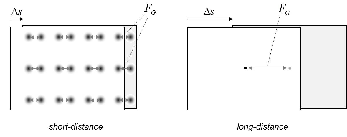
Fig. 1: Illustration of the relevant forces $F_{{}_{G}}$ between the states of a superposed solid for calculating the short-distance and long-distance contribution to the Diósi-Penrose energy.

3.1 Short- and long-distance contributions to the Diósi-Penrose energy

To define the short- and long-distance contributions to the Diósi-Penrose energy of a superposed solid, we regard the solid in Figure 1, whose states are displaced against each other by a distance of $\Delta s$. With the illustration that the Diósi-Penrose energy describes the mechanical work to pull the solid’s states apart from each other over the distance $\Delta s$ against their gravitational attraction (Section 2; Appendix 1), it follows that for small displacements being of the order of the solid’s nuclei’s spatial variation $\sigma$, this work is mainly given by the work to separate corresponding nuclei apart from each other, as illustrated on the left in Figure 1. This follows from the two facts that the nuclei’s masses are concentrated within small areas, and that the gravitational attraction becomes particularly large at small distances ($F_{{}_{G}}$$\propto$$1/r^{2}$). The contribution of this mechanical work to the Diósi-Penrose energy, i.e. the work to separate corresponding nuclei apart from each other, is denoted as the short-distance contribution to the Diósi-Penrose energy. This contribution to the Diósi-Penrose energy depends only on the mass distribution of the solid’s nuclei.

To obtain the complete mechanical work to separate the states of superposed solids apart from each other, we have to regard, in addition to the gravitational attraction of a nucleus to its counterpart in the other state, the attraction of this nucleus to all other nuclei in the other state, which can be at far distance from the regarded nucleus. To calculate this additional mechanical work, which is illustrated on the right in Figure 1, the solid can be approximated as a continuum with a constant mass density, since the concrete mass distributions of the attracting nuclei play no role at long distances. The additional mechanical work resulting from this consideration is called the long-distance contribution to the Diósi-Penrose energy. This depends on the solid’s shape and the direction of the displacement $\Delta s$.

3.2 Short-distance contribution

In this section, we calculate the short-distance contribution to the Diósi-Penrose energy of a superposed solid. We first calculate the mechanical work to pull the states of a superposed single nucleus apart from each other.

Diósi-Penrose energy of a superposed nucleus
The mass distribution of the nucleus shall be approximated by a Gaussian distribution:

$$\rho(\mathbf{x})=m\frac{1}{\sqrt{2\pi\,}^{3}\sigma^{3}}e^{{-\frac{\mathbf{x}^{2}}{2\sigma^{2}}}}\textrm{{~{}~{},~{}~{}~{}~{}~{}~{}~{}~{}~{}~{}~{}~{}}}$$ (6)

where $m$ is the nucleus’ mass and $\sigma$ its spatial variation. The mechanical work to pull the states of a nucleus apart from each other over the distance $\Delta s$ against their gravitational attraction is given by

$$E_{{}_{G}}=\frac{Gm^{2}}{\sqrt{\pi}\sigma}f_{{}_{\sigma}}(\Delta/\sigma)\textrm{{~{}~{}.~{}~{}~{}~{}~{}~{}~{}\footnotesize{Di\'{o}si-Penrose energy of a nucleus}}}$$ (7)

The function $f_{{}_{\sigma}}(x)$ of this result can be approximated for small and large values of $x$ by

$$f_{{}_{\sigma}}(x)\approx\left\{\begin{matrix}~{}~{}\frac{1}{12}x^{2}~{}~{}~{}~{}~{}~{}~{}~{}~{}~{}~{}x<<1\\ 1-\frac{\sqrt{\pi}}{x}~{}~{}~{}~{}~{}~{}x>4\end{matrix}\right.\textrm{{~{}~{}~{}~{}.~{}~{}~{}~{}~{}~{}~{}~{}~{}~{}}}$$ (8)

The function $f_{{}_{\sigma}}(x)$ is shown in Figure 2. The derivation of Equations (7) and (8) is given in Appendix 2.

Spatial variation of the solid’s nuclei
For solids at room temperature, the nuclei’s spatial variation $\sigma$ is mainly determined by the excited acoustical phonons in the solid and is typically of the order of a tenth of an Ångström. The following estimation for the nuclei’s spatial variation $\sigma$ refers, as all other calculations of this paper, to solids at room temperature. However, all our results can easily be adapted to low temperatures by determining the nuclei’s spatial variation $\sigma$ for this case.

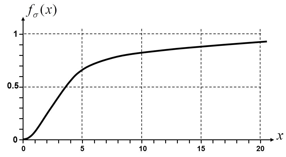
Fig. 2: Function $f_{{}_{\sigma}}(x)$.

The density of states of the phonons in a solid can be described with Debye’s model [17],

$$D_{{}_{Deb}}(\omega)=3N\left\{\begin{matrix}{\frac{3\omega^{2}}{\omega^{3}_{D}}}~{}~{}~{}~{}~{}~{}\omega<\omega_{{}_{D}}\\ ~{}\\ 0~{}~{}~{}~{}~{}~{}~{}~{}~{}\omega>\omega_{{}_{D}}\end{matrix}\right.\textrm{{\footnotesize~{}~{}~{}~{}~{}{with}~{}~{}~{}~{}}}\int^{\infty}_{0}d\omega D_{{}_{Deb}}(\omega)=3N\textrm{{~{}~{},~{}~{}}}$$ (9)

where $\omega_{{}_{D}}$ is the Debye frequency and $N$ the total number of nuclei of the solid. In Appendix 3, it is shown that the Debye model leads to the following spatial variation of the solid’s nuclei:

$$\sigma=\sqrt{\frac{3k_{{}_{B}}T}{\overline{m}}}\frac{1}{\omega_{{}_{D}}}\textrm{{~{}~{},~{}~{}~{}~{}~{}~{}~{}~{}~{}~{}~{}~{}~{}~{}\footnotesize{ spatial variation of nuclei}}}$$ (10)

where $T$ is the temperature, $k_{{}_{B}}$ Boltzmann’s constant and $\overline{m}$ the mean mass of the solids’ nuclei, which is defined by

$$\overline{m}\equiv\sum_{i}\frac{N_{{}_{i}}}{N}m_{{}_{i}}\textrm{{~{}~{}.~{}~{}~{}~{}~{}~{}~{}~{}~{}~{}~{}~{}~{}~{}~{}~{}~{}}}$$ (11)

Here $N_{{}_{i}}$ is the number of nuclei with mass $m_{{}_{i}}$. It is important to note that the nuclei’s spatial variation $\sigma$ (10) is the same for all nuclei, independent of their mass $m_{{}_{i}}$. This results from the fact that for acoustical phonons, which mainly determine the nuclei’s spatial variation $\sigma$, neighbouring nuclei oscillate in phase. The Debye frequency of the solid $\omega_{{}_{D}}$ can on the one hand be calculated from its Debye temperature $\Theta_{{}_{D}}$ by the relation $\hbar\omega_{{}_{D}}$$=$$k_{{}_{B}}\Theta_{{}_{D}}$ [17], which leads to

$$\sigma_{{}_{\Theta}}=\sqrt{\frac{3T}{k_{{}_{B}}\overline{m}}}\frac{\hbar}{\Theta_{{}_{D}}}\textrm{{~{}~{}.~{}~{}~{}~{}~{}~{}~{}~{}~{}~{}~{}~{}~{}~{}~{}~{}~{}}}$$ (12)

The Debye temperature $\Theta_{{}_{D}}$ is usually determined from the temperature profile of the solid’s specific heat [17]. The Debye frequency of the solid $\omega_{{}_{D}}$ can on the other hand be calculated from the solids’ longitudinal and transverse sound velocities $v_{{}_{||}}$ and $v_{{}_{\bot}}$ (Appendix 3), which leads to

$$\sigma_{{}_{v}}=\sqrt{\frac{3k_{{}_{B}}T}{\overline{m}}}\sqrt{\frac{v^{{}^{-3}}_{||}+2v^{{}^{-3}}_{\bot}}{18\pi^{2}}}\bar{g}\textrm{{~{}~{},~{}~{}~{}~{}~{}~{}~{}~{}~{}~{}~{}~{}~{}~{}~{}~{}~{}}}$$ (13)

where $\bar{g}$ is the solid’s mean lattice constant. The mean lattice constant follows from the mean mass $\overline{m}$ and the macroscopic mass density $\rho$ of the solid by

$$\bar{g}~{}{\equiv}~{}\sqrt[3]{\frac{\overline{m}}{\rho}}\textrm{{~{}~{}.~{}~{}~{}~{}~{}~{}~{}~{}~{}~{}~{}~{}~{}~{}\footnotesize{ mean lattice constant}}}$$ (14)

Table 5 shows the nuclei’s spatial variation $\sigma_{{}_{\Theta}}$ calculated from the solid’s Debye temperatures by Equation (12) and the spatial variation $\sigma_{{}_{v}}$ calculated from the solid’s sound velocities by Equation (13) for selected solids at room temperature ($T$$=$$\,300K$). The spatial variations $\sigma_{{}_{\Theta}}$ and $\sigma_{{}_{v}}$ agree quite well and are typically of the order of a tenth of an Ångström ($\sigma$$\approx$ $0.1$Å). All following calculations use the spatial variation calculated from the solid’s Debye temperature (i.e. $\sigma$$\equiv$$\sigma_{{}_{\Theta}}$).

	$\overline{m}[u]$	$\rho[\frac{g}{cm^{3}}]$	$\Theta_{{}_{D}}{[K]}$	$v_{{}_{||}}[\frac{m}{s}]$	$v_{{}_{\bot}}[\frac{m}{s}]$	$\bar{g}[$ Å $]$	$\hat{q}$	$\sigma_{{}_{\Theta}}[$ Å $]$	$\sigma_{{}_{v}}[$ Å $]$	$\frac{\overline{T}^{S}_{G}}{\hbar}[\frac{MHz}{cm^{3}}]$
$Al$	26.98	2.7	398	6420	3040	2.55	1	0.10	0.10	4.3
$Si$	20.09	2.33	654	-	-	2.43	1	0.072	-	3.8
$Fe$	55.85	7.86	453	5960	3240	2.28	1	0.062	0.059	42.1
$Cu$	63.54	10.5	315	5010	2270	2.16	1	0.083	0.074	47.5
$Pb$	207.19	11.4	88	1960	690	3.11	1	0.165	0.194	84.8
$Au$	196.97	19.3	170	3240	1200	2.57	1	0.088	0.094	257.2
$Pt$	195.09	21.4	230	3260	1730	2.47	1	0.065	0.064	380.4
$Ir$	192.2	22.5	430	4825	-	2.42	1	0.035	0.025	731.1
$Al_{{}_{2}}O_{{}_{3}}$	20.39	3.94	1047	10000	-	2.05	1.07	0.044	0.032	11.5
$PZT$	64.94	7.6	274	2910	-	2.42	2.32	0.095	0.072	71.8

Table 1: Characteristic Diósi-Penrose energy density $\overline{T}^{S}_{G}$, spatial variation of nuclei $\sigma_{{}_{\Theta}}$, $\sigma_{{}_{v}}$, quadratic mass factor $\hat{q}$ and mean lattice constant $\bar{g}$ of selected solids calculated from the solid’s sound velocities $v_{{}_{||}}$, $v_{{}_{\bot}}$, Debye temperature $\Theta_{{}_{D}}$, mass density $\rho$ and mean mass $\overline{m}$ for room temperature ($T$$=$$\,300K$).

Table 5 also shows the solid’s mean lattice constant $\bar{g}$, which will play an important role later. The mean lattice constant $\bar{g}$ is typically of the order of two Ångström ($\bar{g}$$\approx$$2$Å) and roughly 20 times larger than the nuclei’s typical spatial variation of $\sigma$$\approx$ $0.1$Å ($\bar{g}/\sigma$$\approx$$20$).

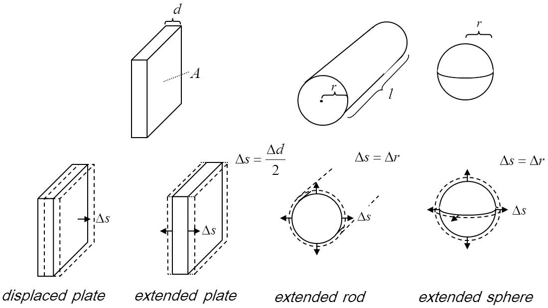
Fig. 3: Cases of superposed solids, in which the solids can have different positions or extensions in the superposed states.

Short-distance contribution for small displacements: $\Delta s$$<<$$\sigma$
The short-distance contribution to the Diósi-Penrose energy of a superposed solid is given by the sum of the Diósi-Penrose energies of its nuclei. This leads with result (7) to

$$E_{{}_{G}}=\frac{G}{\sqrt{\pi}\sigma}(\sum_{i}N_{{}_{i}}m^{2}_{i})<f_{{}_{\sigma}}(\Delta s/\sigma)>\textrm{{~{}~{},~{}~{}~{}~{}~{}~{}~{}~{}~{}~{}~{}~{}~{}~{}~{}~{}~{}}}$$ (15)

where $<$$f_{{}_{\sigma}}(\Delta s/\sigma)$$>$ denotes the averaging over the function $f_{{}_{\sigma}}(\Delta s/\sigma)$. This averaging becomes necessary when the displacements $\Delta s$ between belonging nuclei are not the same for all nuclei. This is the case when e.g. the solids have different extensions in the superposed states. In our calculations of the Diósi-Penrose energy of superposed solids, we regard the four cases in Figure 3, which are referred to as displaced plate, extended plate, extended rod and extended sphere. In the displaced plate, the solid has in the two states of the superposition slightly different positions. In the other three cases, the extended plate, rod and sphere, the solid has in the two states slightly different extensions, as illustrated in Figure 3.

For displacements much smaller than the nuclei’s spatial variation ($\Delta s$$<<$$\sigma$), where the function $f_{{}_{\sigma}}(x)$ (8) quadratically increases, Equation (15) can be converted with the help of $\sum_{{}_{i}}$$N_{{}_{i}}m_{{}_{i}}$$=$$\rho V$ to

$$E_{{}_{G}}=\frac{\alpha_{{}_{geo}}}{12\sqrt{\pi}}GV\hat{q}\rho^{2}\frac{\bar{g}^{3}}{\sigma}\left(\frac{\Delta s}{\sigma}\right)^{2}~{}~{}~{}~{}~{}~{}~{}\Delta s<<\sigma\textrm{{~{}~{},~{}~{}~{}~{}~{}~{}~{}~{}~{}~{}~{}~{}~{}~{}~{}~{}~{}}}$$ (16)

where $V$ is the solid’s volume, $\alpha_{{}_{geo}}$ the so-called geometric factor and $\hat{q}$ the so-called quadratic mass factor of the solid. The geometric factor depends on the solid’s shape and the direction of the displacement and is for the four cases in Figure 3 given by

$$\begin{matrix}{\alpha_{{}_{d-pl}}={1}}\textrm{{\footnotesize~{}~{}~{}~{}~{}~{}{displaced plate}~{}~{}~{}}}\\ {\alpha_{{}_{e-pl}}={1/3}}\textrm{{\footnotesize~{}~{}~{}{extended plate}~{}~{}~{}}}\\ {\alpha_{{}_{e-ro}}={1/2}}\textrm{{\footnotesize~{}~{}~{}{extended rod}~{}~{}~{}~{}~{}}}\\ {\alpha_{{}_{e-sp}}={3/5}}\textrm{{\footnotesize~{}~{}~{}{extended sphere}}}\end{matrix}\textrm{{~{}~{}.~{}~{}~{}~{}~{}~{}~{}~{}~{}~{}~{}~{}~{}~{}\footnotesize{geometric factor {\small$\alpha_{{}_{geo}}$} }}}$$ (17)

The quadratic mass factor is defined by

$$\hat{q}~{}\equiv~{}\frac{\sum_{i}N_{{}_{i}}m^{2}_{i}}{\sum_{i}N_{{}_{i}}m_{{}_{i}}\overline{m}}\textrm{{~{}~{}.~{}~{}~{}~{}~{}~{}~{}~{}~{}~{}~{}~{}~{}~{}\footnotesize{ quadratic mass factor}}}$$ (18)

For solids consisting of only one chemical element, the quadratic mass factor is one ($\hat{q}\,$$=$$1$). Table 5 shows the quadratic mass factors $\hat{q}$ of the selected solids.

The quadratic increase of the short-distance contribution to the Diósi-Penrose energy (16) with the displacement ($E_{{}_{G}}$$\propto$$\Delta s^{2}$) at displacements much smaller than the nuclei’s spatial variation ($\Delta s$$<<$$\sigma$) is generic, since the attracting gravitational force between the nuclei can be linearised for small displacements.

Short-distance contribution for large displacements: $\Delta s$$>$$4\sigma$
For large displacements with $\Delta s$$>$$4\sigma$, Equation (15) yields

$$E_{{}_{G}}=\frac{1}{\sqrt{\pi}}GV\hat{q}\rho^{2}\frac{\bar{g}^{3}}{\sigma}F_{{}_{geo}}(\frac{\Delta s}{\sigma})~{}~{}~{}~{}~{}~{}~{}~{}\Delta s>4\sigma\textrm{{~{}~{},~{}~{}~{}~{}~{}~{}~{}~{}~{}~{}~{}~{}~{}~{}~{}~{}~{}}}$$ (19)

where $F_{{}_{geo}}(x)$ is the so-called geometric function. The geometric functions of the displaced and extended plate are given by

$$\begin{split}\begin{matrix}F_{{}_{d-pl}}(x)=1-\frac{\sqrt{\pi}}{x}\textrm{{\footnotesize~{}~{}~{}~{}~{}~{}~{}~{}~{}~{}~{}~{}~{}~{}~{}~{}~{}~{}~{}~{}~{}~{}~{}~{}~{}~{}~{}~{}~{}~{}~{}~{}~{}~{}~{}~{}~{}~{}~{}~{}{displaced plate}}}\\ ~{}\\ F_{{}_{e-pl}}(x)=1-\frac{2+\sqrt{\pi}/2-\sqrt{\pi}ln(4)}{x}-{\sqrt{\pi}}\frac{ln(x)}{x}\textrm{{\footnotesize~{}~{}~{}{extended plate}}}\end{matrix}\textrm{{~{}~{}~{}.}}\\ ~{}\\ \textrm{{~{}~{}~{}~{}~{}~{}~{}~{}~{}~{}~{}~{}~{}~{}~{}~{}~{}~{}~{}~{}~{}~{}~{}~{}~{}~{}~{}~{}~{}~{}~{}~{}~{}~{}~{}~{}~{}~{}~{}~{}\footnotesize{geometric function {\small$F_{{}_{geo}}(x)$}}}}\end{split}$$ (20)

For large values of $x$, the geometric functions converge to one ($lim_{{}_{x\rightarrow\infty}}F_{{}_{geo}}(x)$$=$$1$). That the Diósi-Penrose energy converges against a constant value for large displacement is generic for the short-distance contribution, since the attracting gravitational force between the nuclei vanishes for large displacements $\Delta s$. The geometric functions of the extended rod and sphere can also be expressed by analytical expressions, but are not needed in further discussions.

Short-distance contribution for small and large displacements
Equations (16) and (19) for the short-distance contribution to the Diósi-Penrose energy for small and large displacements $\Delta s$ can be brought together as follows:

$$\begin{split}E^{{}^{Ss}}_{G_{geo}}(\Delta s,\sigma,\bar{g},\hat{q},\rho,V)=\overline{T}^{S}_{G}V\cdot\left\{\begin{matrix}{\frac{\alpha_{{}_{geo}}}{12}(\frac{\Delta s}{\sigma})^{2}}~{}~{}~{}~{}~{}\Delta s<<\sigma\\ ~{}\\ {F_{{}_{geo}}(\frac{\Delta s}{\sigma})}~{}~{}~{}~{}~{}~{}~{}\Delta s>4\sigma\end{matrix}\right.~{}~{}~{}~{},~{}~{}~{}~{}~{}~{}~{}~{}~{}~{}~{}~{}~{}~{}~{}~{}~{}~{}~{}~{}~{}~{}~{}~{}~{}\\ \textrm{{~{}~{}~{}~{}~{}~{}~{}~{}~{}~{}~{}~{}~{}~{}~{}~{}~{}~{}~{}~{}~{}~{}~{}~{}~{}~{}~{}~{}~{}~{}~{}~{}~{}~{}~{}~{}~{}~{}\footnotesize{short-distance contribution to the Di\'{o}si-Penrose energy of a solid}}}\end{split}$$ (21)

where $\overline{T}^{S}_{G}$ is the so-called characteristic Diósi-Penrose energy density of a solid, which is given by

$$\overline{T}^{S}_{G}~{}\equiv~{}\frac{G\hat{q}\rho^{2}\bar{g}^{3}}{\sqrt{\pi}\sigma}\textrm{{~{}~{}.~{}~{}~{}~{}~{}~{}~{}\footnotesize{characteristic Di\'{o}si-Penrose energy density of a solid }}}$$ (22)

The characteristic Diósi-Penrose energy density multiplied by the solid’s volume $\overline{T}^{S}_{G}V$ describes the short-distance contribution to the Diósi-Penrose energy for an infinitely large displacement ($\Delta s$$\rightarrow$$\infty$). Table 5 shows the characteristic Diósi-Penrose energy density divided by Planck’s constant $\overline{T}^{S}_{G}/\hbar$ for the selected solids, which describe according to the Diósi-Penrose criterion (1) a decay rate per volume. This quantity ranges from $4MHz/cm^{3}$ for aluminium, to over $42MHz/cm^{3}$ for iron, and up to $730MHz/cm^{3}$ for iridium.

Differences in monocrystals
Equation (21) for the short-distance contribution to the Diósi-Penrose energy assumes amorphous crystals. In monocrystals, which are displaced along one of their axes, one obtains a different behaviour. When the nuclei’s positions of the displaced solid exactly coincide with those of the not-displaced one, the mechanical work for this displacement is zero, i.e. the Diósi-Penrose energy does not monotonically increase with $\Delta s$, but oscillates with a period of $\Delta s$$=$$g$. In amorphous crystals, the chance that the position of a displaced nucleus coincides with the position of a not displaced one is of the order of $(2\sigma/\bar{g})^{3}$, which is one in a thousand for the typical ratio of $\bar{g}/\sigma$$\approx$$20$.

3.3 Long-distance contribution

The calculation of the long-distance contribution to the Diósi-Penrose energy for the four cases of Figure 3 is given in Appendix 4, and yields

$$\begin{split}E^{{}^{S\,l}}_{G_{geo}}(\Delta s,\rho,V)=2\pi\alpha_{{}_{geo}}GV\rho^{2}\Delta s^{2}~{}~{}~{}~{}~{}~{}~{}~{}~{}~{}~{}~{}~{}~{}~{}~{}~{}~{}~{}~{}~{}~{}~{}~{}~{}~{}~{}~{}~{}~{}~{}~{}~{}~{}~{}~{}~{}~{}~{}~{}~{}~{}~{}~{}~{}\\ \textrm{{~{}~{}.~{}~{}~{}~{}~{}~{}~{}~{}~{}~{}~{}~{}~{}~{}~{}~{}~{}~{}~{}~{}~{}~{}~{}\footnotesize{long-distance contribution to the Di\'{o}si-Penrose energy of a solid}}}\end{split}$$ (23)

for displacements $\Delta s$ being much smaller than the solid’s extension ($\Delta s$$<<$$\sqrt[3]{V}$). The geometric factors $\alpha_{{}_{geo}}$ of this result are given by Equation (17) and are exactly the same as those found for the short-distance contribution to the Diósi-Penrose energy for small displacements (16). The quadratic increase of the long-distance contribution to the Diósi-Penrose energy (23) with the displacement at displacements much smaller than the solid’s extension is generic, since the attracting gravitational force between the solids can be linearised for $\Delta s$$<<$$\sqrt[3]{V}$.

Proportionality between Diósi-Penrose energy and volume is not generic
It is important to note that the proportionality between the solid’s long-distance contribution to the Diósi-Penrose energy $E_{{}_{G}}$ and the solid’s volume $V$ (Equation 23) is, in contrast to the short-distance contribution to the Diósi-Penrose energy (Equation 21), not generic. For a rod being displaced parallel to its direction, the long-distance contribution to the Diósi-Penrose energy does not linearly increase with the rod’s length. It converges to a constant value for large lengths of the rod.

3.4 Common view on the short- and long-distance contribution

In the four cases of Figure 3, where the solid’s long-distance contribution to the Diósi-Penrose energy is proportional to the solid’s volume, and which are sufficient for the practical applications discussed here, Equations (21) and (23) for the short- and long-distance contributions can be joined as follows:

$$\begin{split}E^{{}^{S}}_{G_{geo}}(\Delta s,\sigma,\bar{g},\hat{q},\rho,V)=\overline{T}^{S}_{G}V\cdot\left\{\begin{matrix}{(1+\chi)\frac{\alpha_{{}_{geo}}}{12}(\frac{\Delta s}{\sigma})^{2}}~{}~{}~{}~{}~{}~{}~{}~{}~{}~{}~{}~{}~{}~{}~{}\Delta s<<\sigma\\ ~{}\\ {F_{{}_{geo}}(\frac{\Delta s}{\sigma})+\alpha_{{}_{geo}}\xi(\frac{\Delta s}{\bar{g}})^{2}}~{}~{}~{}~{}~{}~{}~{}\Delta s>4\sigma\end{matrix}\right.~{}~{}~{}~{},~{}~{}~{}~{}~{}~{}~{}~{}~{}~{}~{}\\ \textrm{{~{}~{}~{}~{}~{}~{}~{}~{}~{}~{}~{}~{}~{}~{}~{}~{}~{}~{}~{}~{}~{}~{}~{}~{}~{}~{}~{}\footnotesize{Di\'{o}si-Penrose energy of a solid}}}\end{split}$$ (24)

where the factors $\chi$ and $\xi$ are given by

$$\chi\equiv\frac{24\pi^{3/2}}{\hat{q}(\bar{g}/\sigma)^{3}}~{}~{}~{}~{}~{},~{}~{}~{}~{}~{}\xi\equiv\frac{2\pi^{3/2}}{\hat{q}(\bar{g}/\sigma)}\textrm{{~{}~{}~{}~{}~{}.~{}~{}~{}~{}~{}~{}~{}~{}~{}~{}~{}~{}~{}~{}\footnotesize{factors $\chi$, $\xi$}}}$$ (25)

For the typical values of $\hat{q}\,$$\approx$$1$ and $\bar{g}/\sigma$$\approx$$20$ these factors are

$$\chi\approx\frac{1}{60}~{}~{}~{}~{}~{},~{}~{}~{}~{}~{}\xi\approx\frac{1}{2}\textrm{{~{}~{}~{}~{}.~{}~{}~{}~{}~{}~{}~{}~{}~{}~{}~{}~{}~{}~{}~{}~{}~{}~{}~{}~{}~{}~{}~{}}}$$ (26)

For displacements much smaller than the nuclei’s spatial variation ($\Delta s$$<<$$\sigma$), the short- and long-distance contributions both quadratically increase with the displacement $\Delta s$. However, the long-distance contribution is by a factor of $\chi$$\approx$$\frac{1}{60}$ smaller, which allows us to neglect the long-distance contribution in this regime. This means that for $\Delta s$$<<$$\sigma$ the Diósi-Penrose energy is mainly determined by the solid’s microscopic mass distribution resulting from its nuclei. For displacements much larger than the solid’s mean lattice constant ($\Delta s$$>>$$\bar{g}$), the long-distance contribution dominates the Diósi-Penrose energy. In this regime, the solid can be regarded as a continuum with a constant mass density $\rho$ for the calculation of the Diósi-Penrose energy. In the intermediate regime, both contributions, i.e. short- and long-distance, have to be taken into account.

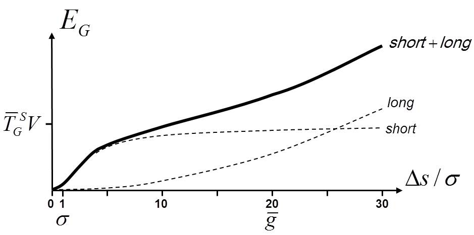
Fig. 4: Dependency of the short- and the long-distance contributions to the Diósi-Penrose energy on the displacement $\Delta s$ for a displaced plate consisting of a solid with $\hat{q}\,$$=$$1$ and $\bar{g}/\sigma$$=$$20$.

Figure 4 visualises the dependency of the short- and long-distance contributions to the Diósi-Penrose energy on the displacement $\Delta s$ for a displaced plate consisting of a solid with $\hat{q}\,$$=$$1$ and $\bar{g}/\sigma$$=$$20$. The figure shows that the short-distance contribution dominates for $\Delta s$$<<$$\sigma$ and the long-distance contribution for $\Delta s$$>>$$\bar{g}$. On the interval $[5\sigma,\bar{g}]$ the Diósi-Penrose energy is approximately given by $\overline{T}^{S}_{G}V$. From the above discussion, it follows that the Diósi-Penrose energy of a superposed solid can be estimated by the following rule of thumb:

$$\begin{split}E_{{}_{G}}\approx\left\{\begin{matrix}{\frac{\alpha_{{}_{geo}}}{12}\overline{T}^{S}_{G}V(\frac{\Delta s}{\sigma})^{2}}~{}~{}~{}~{}~{}~{}~{}~{}~{}\Delta s<<\sigma\\ ~{}\\ {\overline{T}^{S}_{G}V}~{}~{}~{}~{}~{}~{}~{}~{}~{}~{}~{}~{}~{}5\sigma<\Delta s\leq\bar{g}\\ ~{}\\ {\alpha_{{}_{geo}}\xi\overline{T}^{S}_{G}V(\frac{\Delta s}{\bar{g}})^{2}}~{}~{}~{}~{}~{}~{}~{}\Delta s>>\bar{g}\end{matrix}\right.~{}~{}~{}~{}.~{}~{}~{}~{}~{}~{}~{}~{}~{}~{}~{}~{}~{}~{}~{}~{}~{}~{}~{}~{}~{}~{}~{}~{}~{}~{}~{}~{}~{}~{}~{}~{}~{}~{}~{}~{}~{}\\ \\ \textrm{{~{}~{}~{}~{}~{}~{}~{}~{}~{}~{}~{}~{}~{}~{}~{}~{}~{}~{}~{}~{}~{}~{}~{}~{}~{}~{}~{}~{}~{}~{}~{}~{}~{}~{}~{}~{}\footnotesize{rule of thumb for the Di\'{o}si-Penrose energy of a superposed solid }}}\end{split}$$ (27)

The characteristic quantities of a solid, which are needed for calculating the Diósi-Penrose energy, are its characteristic Diósi-Penrose energy density $\overline{T}^{S}_{G}$, its mean lattice constant $\bar{g}$, the spatial variation of its nuclei $\sigma$ and the quadratic mass factor $\hat{q}$. From Table 5, which shows these quantities for the selected solids, it follows that the solids mainly differ by their characteristic Diósi-Penrose energy densities $\overline{T}^{S}_{G}$, which scale with the square of the solid’s mass densities $\rho$. In the long-distance regime ($\Delta s$$>>$$\bar{g}$) only the solid’s mass density $\rho$ is needed for calculating the Diósi-Penrose energy, as one can see from Equation (23). Beside these, the solid characterising quantities, the Diósi-Penrose energy depends on the geometric factor $\alpha_{{}_{geo}}$, the solid’s volume $V$ and the displacement $\Delta s$.

3.5 Differences in Diósi’s approach

In Diósi’s approach the operator for calculating the mass density must, according to Equation (5), be smeared by a characteristic radius $\sigma_{{}_{D}}$. This characteristic radius $\sigma_{{}_{D}}$ was originally chosen by Diósi to be in the order of the nucleon’s radius, i.e. $\sigma_{{}_{D}}$$\approx$$10^{-13}cm$ [15], and was later revised by Ghirardi to a much greater value of $\sigma_{{}_{D}}$$\approx$$10^{-5}cm$ [16]. This correction was necessary to avoid a too-strong permanent increase of total energy [16]. Since the characteristic radius $\sigma_{{}_{D}}$ is much larger than the solid’s mean lattice constant of $\bar{g}\,$$\approx$$\,2\cdot 10^{-8}cm$, the solid’s microscopic mass distribution plays no role. This allows one to idealise the solid as a continuum with constant mass density; a result that has already been pointed out by Diósi himself [19]. This means that the short-distance contribution to the Diósi-Penrose energy must be omitted in Diósi’s approach. This leads in the short-distance regime ($\Delta s$$<<$$\sigma$) to a factor of $\chi$$\approx$$\frac{1}{60}$ smaller Diósi-Penrose energy and therefore to typically 60 times larger lifetimes $T_{{}_{G}}$ of the solid. In the long-distance regime ($\Delta s$$>>$$\bar{g}$), in which the short-distance contribution can be neglected and the solid can be idealised as a continuum, Diósi’s approach leads to the same results as discussed in Section 3.4.

3.6 Combinations of solids

In the application of our results to detector components in Section 4, we have to consider combinations of different solids. This is the case in e.g. the plate capacitor of Figure 5, whose dielectric is compressed by the electrical forces between its plates. The compression of the capacitor’s dielectric can be discussed with the extended plate, and the movement of the capacitor’s plates with the displaced plate in Figure 3. In this section, we suggest that the total long-distance contribution to the Diósi-Penrose energy of such combinations is not simply the sum of its parts, which is the case for the total short-distance contribution to the Diósi-Penrose energy. In Appendix 5, it is shown that one obtains interference terms for the total long-distance contribution to the Diósi-Penrose energy, in addition to the sum of the long-distance contributions of the parts. Furthermore, it is shown that these interference terms vanish for the plate capacitor in Figure 5, when the size of its plates is much greater than the thicknesses of its dielectric and its plates. In the following calculations of the Diósi-Penrose energies of detector components, these interference terms are neglected.

4 Diósi-Penrose criterion for detector components in quantum superpositions

In this section, we apply the results for solids in quantum superpositions to the components of the single-photon detector that will be discussed in Section 5. These are plate capacitors, photodiodes, resistors, wires and piezoactuators. In Section 4.1, we discuss plate capacitors, which will be used for biasing the avalanche photodiodes. In Section 4.2, we derive formulae for resistors and wires, which can be adapted to photodiodes also. In Section 4.3, we discuss a piezoactuator, with which the detector’s lifetime can be shortened.

4.1 Plate capacitors

In this section we calculate the Diósi-Penrose energy of a plate capacitor in a superposition of two states, in which different voltages of $V$ and $V$$+$$\Delta V$ are applied to it. There are three effects contributing to the capacitor’s Diósi-Penrose energy, which are the compression of its dielectric by the electric force between the plates, the polarisation of its dielectric, and the Diósi-Penrose energy resulting from the masses of the electric charge on its plates. The discussion in Section 5.1 will show that the compression of the capacitors dielectric is the dominating effect, and that the other two effects can be neglected.

Fig. 5: Plate capacitor, whose dielectric is compressed by a distance of $\Delta s$ due to the electric force between its plates.

Compression of the dielectric
We consider the plate capacitor in Figure 5, whose plates have an area of $A$ and a thickness of $d_{{}_{m}}$, and whose dielectric has a thickness of $d$. When the capacitor is charged, the electric force between its plates compresses its dielectric slightly. How the dielectric’s thickness $d$ changes with the pressure $P$ of the plates on the dielectric is described by the modulus of elasticity $E_{{}_{e}}$ according to the following relation [20]:

$$\frac{\Delta d}{d}=-\frac{\Delta P}{E_{{}_{e}}}\textrm{{~{}~{}.~{}~{}~{}~{}~{}~{}~{}~{}~{}~{}~{}~{}~{}~{}~{}~{}~{}}}$$ (28)

A change of the capacitor’s voltage by $\Delta V$ displaces its plates by a distance of $\Delta s$ as follows ($\Delta s$$=$$\Delta d/2$):

$$\Delta s=\frac{\epsilon_{{}_{0}}\epsilon^{2}_{r}\Delta V}{E_{{}_{e}}d}\textrm{{~{}~{},~{}~{}~{}~{}~{}~{}~{}~{}~{}~{}~{}~{}~{}~{}~{}~{}~{}}}$$ (29)

where $\epsilon_{{}_{0}}$ is the electric constant and $\epsilon_{{}_{r}}$ the dielectric’s relative permittivity. In Appendix 5 it is shown that the Diósi-Penrose energy of the capacitor (staying in a superposition of states with voltages of $V$ and $V$$+$$\Delta V$) is the sum of the Diósi-Penrose energies of the dielectric and of the two plates when the size of its plates is much greater than the thicknesses of its dielectric and its plates ($\sqrt{A}$$>>$$d,d_{{}_{m}}$). The Diósi-Penrose energy resulting from the compression of the dielectric corresponds to the extended plate in Figure 3, and the Diósi-Penrose energy resulting from the displacements of the plates to the displaced plate in Figure 3. This leads with Equation (24) to:

$$E_{{}_{G}}=E^{{}^{S}}_{G_{e-pl}}(\Delta s,\sigma_{{}_{d}},\bar{g}_{{}_{d}},\hat{q}_{{}_{d}},\rho_{{}_{d}},Ad)+2E^{{}^{S}}_{G_{d-pl}}(\Delta s,\sigma_{{}_{m}},\bar{g}_{{}_{m}},\hat{q}_{{}_{m}},\rho_{{}_{m}},Ad_{{}_{m}})~{}~{}~{}{\sqrt{A}>>d,d_{{}_{m}}}\textrm{{,}}$$ (30)

where the indices $d$ and $m$ of the nuclei’s spatial variation $\sigma$, the mean lattice constant $\bar{g}$, the quadratic mass factor $\hat{q}$ and the mass density $\rho$ refer to the materials of the capacitor’s dielectric and its metal plates respectively. In the single-photon detector discussed in Section 5.1, the displacements of the capacitor’s plates $\Delta s$ are so small that one can restrict to the short-distance contribution to the Diósi-Penrose energy, which simplifies Equation (30) to:

$$E_{{}_{G}}\approx\frac{A}{12}({\frac{1}{3}}\frac{d\overline{T}^{d}_{G}}{\sigma^{2}_{d}}+2\frac{d_{{}_{m}}\overline{T}^{m}_{G}}{\sigma^{2}_{m}})\Delta s^{2}~{}~{}~{}~{}~{}~{}~{}~{}\Delta s<<\sigma_{{}_{d}},\sigma_{{}_{m}}\textrm{{~{}~{},~{}~{}~{}~{}~{}~{}~{}~{}~{}~{}~{}~{}~{}~{}~{}~{}~{}}}$$ (31)

where $\overline{T}^{d}_{G}$ and $\overline{T}^{m}_{G}$ are the characteristic Diósi-Penrose energy densities of the capacitor’s dielectric and of its plates. With the Diósi-Penrose criterion ($T_{{}_{G}}$$\approx$$\,\hbar/E_{{}_{G}}$) and Equation (31), we can now estimate how long the capacitor will stay in a superposition of states with voltages of $V$ and $V$$+$$\Delta V$. The lifetime $T_{{}_{G}}$ of this calculation has to be compared to the settling time $\Delta t$ the capacitor’s plates’ need for being displaced by a voltage change of $\Delta V$, where the settling time $\Delta t$ has to be much smaller than the superposition’s lifetime $T_{{}_{G}}$ ($\Delta t$$<<$$T_{{}_{G}}$). The settling time $\Delta t$ follows from the solid’s longitudinal sound velocity $v_{{}_{||}}$ by the relation:

$$\Delta t\approx\frac{d}{2v_{{}_{||}}}\textrm{{~{}~{}.~{}~{}~{}~{}~{}~{}~{}~{}~{}~{}~{}~{}~{}~{}~{}~{}~{}}}$$ (32)

Polarisation of the dielectric
The physical origin of the dielectric’s relative permittivity $\epsilon_{{}_{r}}$ is that charged particles are displaced when an electric field is applied. These displacements also contribute to the capacitor’s Diósi-Penrose energy. The discussion in Section 5.1 will show that the displacements $\Delta s$ resulting from the dielectric’s polarisation are much smaller than those resulting from its compression. The displacements $\Delta s$ resulting from the dielectric’s polarisation can be estimated by assuming that the dielectric consists of two ions with charges of $+e$, $-e$ and identical masses $m$. The displacement of the ions $\Delta s$ is then given by

$$\Delta s=\frac{\epsilon_{{}_{0}}(\epsilon_{{}_{r}}-1)m}{e\rho}\frac{\Delta V}{d}\textrm{{~{}~{}.~{}~{}~{}~{}~{}~{}~{}~{}~{}~{}~{}~{}~{}~{}~{}~{}~{}}}$$ (33)

Diósi-Penrose energy resulting from the capacitor’s charge
When the capacitor is charged, the weight of its plates will slightly increase due to the electrons’ masses $m_{{}_{e}}$. The Diósi-Penrose energy resulting from this effect is given by

$$E_{{}_{G}}=\frac{2\pi G\epsilon^{2}_{0}m^{2}_{e}\epsilon^{2}_{r}A}{e^{2}d}\Delta V^{2}\textrm{{~{}~{}.~{}~{}~{}~{}~{}~{}~{}~{}~{}~{}~{}~{}~{}~{}~{}~{}~{}}}$$ (34)

4.2 Wires and resistors

In this section we consider wires and resistors in quantum superpositions. We assume that in one state of the superposition a current $I(t)$ has flowed through the component and in the other state not. The temperature increase $\Delta T$ resulting from the heat energy $\Delta W$ generated by the current flow $I(t)$ from $t$$=$$0$ until $t$$=$$t_{{}_{s}}$ is given by

$$\Delta T=\frac{\bar{g}^{3}R^{2}}{3k_{{}_{B}}\rho_{{}_{\Omega}}l^{2}}\int^{t_{s}}_{0}dtI(t)^{2}\textrm{{~{}~{},~{}~{}~{}~{}~{}~{}~{}~{}~{}~{}~{}~{}~{}~{}~{}~{}~{}}}$$ (35)

where $l$ and $r$ are the length and radius of the wire (resistor), $\rho_{{}_{\Omega}}$ its electrical resistivity and $R$ its resistance. The temperature increases $\Delta T$ causes a thermal expansion of the component, which leads in the case of a wire to so-called longitudinal and transverse displacements $\Delta s_{{}_{||}}$ and $\Delta s_{{}_{\bot}}$, which are illustrated in Figure 6.

Fig. 6: Illustration of the longitudinal and transverse displacements $\Delta s_{{}_{||}}$ and $\Delta s_{{}_{\bot}}$ occurring when wires thermally expand, and an illustration of the wire’s effective length $l_{{}_{e}}$.

The longitudinal displacement $\Delta s_{{}_{||}}$ increases proportionally with the wire’s radius $r$, and the transverse displacement $\Delta s_{{}_{\bot}}$ with the wire’s so-called effective length $l_{{}_{e}}$, whose definition becomes obvious with the illustration in Figure 6. The displacements $\Delta s_{{}_{||}}$ and $\Delta s_{{}_{\bot}}$ can be calculated with the help of the solid’s thermal expansion coefficient $\alpha_{{}_{L}}$ as follows [20]:

$$\begin{split}\Delta s_{{}_{||}}=\alpha_{{}_{L}}\frac{l_{{}_{e}}}{2}\Delta T\\ \Delta s_{{}_{\bot}}=~{}\alpha_{{}_{L}}r\Delta T\end{split}\textrm{{~{}~{}~{}~{}.~{}~{}~{}~{}~{}~{}~{}~{}~{}~{}~{}~{}~{}~{}~{}~{}~{}}}$$ (36)

The long-distance contribution to the wire’s Diósi-Penrose energy is given by Equation (23) with $\Delta s$$=$$\Delta s_{{}_{\bot}}$ and $\alpha_{{}_{geo}}$$=$$\frac{1}{2}$ for the extended rod. The short-distance contribution to the wire’s Diósi-Penrose energy is given by Equation (21) with $\Delta s$$=$$\Delta s_{{}_{||}}$ and $\alpha_{{}_{geo}}$$=$$\frac{1}{3}$ for the extended plate. Both contributions together yield

$$E_{{}_{G}}\approx E^{{}^{Ss}}_{G_{e-pl}}(\Delta s_{{}_{||}},\sigma,\bar{g},\hat{q},\rho,\pi r^{2}l)+E^{{}^{S\,l}}_{G_{e-ro}}(\Delta s_{{}_{\bot}},\rho,\pi r^{2}l)\textrm{{~{}~{}.~{}~{}~{}~{}~{}~{}~{}~{}~{}~{}~{}~{}~{}~{}~{}~{}~{}}}$$ (37)

The discussion of the single-photon detector in Section 5.1 will show that the thermal expansions of the wires and resistors are so small that one can restrict to the short-distance contribution, which simplifies Equation (37) to

$$E_{{}_{G}}\approx{\frac{1}{36}}\overline{T}^{S}_{G}\pi r^{2}l\left(\frac{\Delta s_{{}_{||}}}{\sigma}\right)^{2}~{}~{}~{}~{}~{}~{}\Delta s_{{}_{||}}<<\sigma\textrm{{~{}~{}.~{}~{}~{}~{}~{}~{}~{}~{}~{}~{}~{}~{}~{}~{}~{}~{}~{}}}$$ (38)

The settling time $\Delta t$ for the wire’s longitudinal displacement $\Delta s_{{}_{||}}$ is given by

$$\Delta t\approx\frac{l_{{}_{e}}}{2v_{{}_{||}}}\textrm{{~{}~{},~{}~{}~{}~{}~{}~{}~{}~{}~{}~{}~{}~{}~{}~{}~{}~{}~{}}}$$ (39)

where $v_{{}_{||}}$ is the wire’s longitudinal sound velocity.

Metal-film resistors shorten the lifetime
In this section, we discuss the question of how to construct a resistor to obtain a low Diósi-Penrose energy, respective long lifetime of the resistor ($T_{{}_{G}}$$=$$\,\hbar/E_{{}_{G}}$). The Diósi-Penrose energy of a resistor increases with the inverse of its electrical resistivity $\rho_{{}_{\Omega}}$, when the resistor’s resistance $R$ and length $l$ is kept constant:

$$E_{{}_{G}}~{}\propto~{}\frac{1}{\rho_{{}_{\Omega}}}\textrm{{~{}~{}.~{}~{}~{}~{}~{}~{}~{}~{}~{}~{}~{}~{}~{}~{}~{}~{}~{}}}$$ (40)

To obtain a long lifetime, it is recommended not to use commercially available metal-film resistors, which use thin metal layers to create their resistance. In Section 5.1, in which we show how long a single-photon detector can stay in a superposition, we therefore construct the resistor by means of a rod of doped silicon with an electrical resistivity of approximately $\rho_{{}_{\Omega}}$$\approx$$1\Omega cm$ instead of a metal-film resistor with electrical resistivities of the order of $10^{-5}\Omega cm$ to $10^{-6}\Omega cm$.

4.3 Piezoactuators

In this section, we calculate the Diósi-Penrose energy of a piezoactuator in a quantum superposition. We assume that a voltage of $V$ is applied to the actuator in one state of the superposition, and no voltage in the other state. Since piezoactuators can generate large displacements $\Delta s$, they can be used to shorten the lifetimes of quantum superpositions, as done by Salart et al. [13] to enforce reduction in an EPR experiment. We now regard the simplest variant of a piezoactuator, which consists of a plate capacitor with a piezo as dielectric, as illustrated in Figure 7. When a voltage is applied, the piezo presses the capacitor’s plates apart from each other by the converse piezoelectric effect. Commercially available piezoactuators consist of several layers of such piezo capacitors to achieve larger displacements [21]. The following results can easily be adapted for more than one piezo layer.

Fig. 7: Simple piezoactuator consisting of a plate capacitor with a piezo as dielectric.

To simplify discussion, we regard piezos in which only the $d_{{}_{33}}$-component of the matrix for the converse piezoelectric effect is relevant. The $d_{{}_{33}}$-component describes how much the piezo’s extension in the z-direction changes when an electrical field in the same direction is applied by the following relation [21]:

$$\frac{\Delta d}{d}=d_{{}_{33}}E\textrm{{~{}~{},~{}~{}~{}~{}~{}~{}~{}~{}~{}~{}~{}~{}~{}~{}~{}~{}~{}}}$$ (41)

where $E$ is the applied electric field and $d$ the piezo’s thickness. When a voltage of $V$ is applied, the piezo capacitor’s plates move by [21]

$$\Delta s=\frac{d_{{}_{33}}}{2}V\textrm{{~{}~{}.~{}~{}~{}~{}~{}~{}~{}~{}~{}~{}~{}~{}~{}~{}~{}~{}~{}}}$$ (42)

The Diósi-Penrose energy of the piezo capacitor is the same as that of the plate capacitor (30) discussed in Section 4.1:

$$E_{{}_{G}}=E^{{}^{S}}_{G_{e-pl}}(\Delta s,\sigma_{{}_{p}},\bar{g}_{{}_{p}},\hat{q}_{{}_{p}},\rho_{{}_{p}},Ad)+2E^{{}^{S}}_{G_{d-pl}}(\Delta s,\sigma_{{}_{m}},\bar{g}_{{}_{m}},\hat{q}_{{}_{m}},\rho_{{}_{m}},Ad_{{}_{m}})~{}~{}~{}{\sqrt{A}>>d,d_{{}_{m}}}\textrm{{.}}$$ (43)

The index $p$ in this expression refers to the piezo. For displacements much larger than the mean lattice constant ($\Delta s$$>>$$\bar{g}$), which can easily be achieved with piezo actuators, Equation (43) simplifies to

$$E_{{}_{G}}=2\pi GA({\frac{1}{3}}d\rho^{2}_{p}+2d_{{}_{m}}\rho^{2}_{m})\Delta s^{2}~{}~{}~{}~{}~{}~{}~{}\Delta s>>\bar{g}_{{}_{p}},\bar{g}_{{}_{m}}\textrm{{~{}~{}.~{}~{}~{}~{}~{}~{}~{}~{}~{}~{}~{}~{}~{}~{}~{}~{}~{}}}$$ (44)

The settling time $\Delta t$ of the piezo capacitor for becoming displaced depends on the frequency dependency of the piezo electric $d_{{}_{33}}$-coefficient, in addition to the aforementioned effect resulting from the finite sound velocities of the piezo $v^{{}^{p}}_{||}$ and the metal plates $v^{{}^{m}}_{||}$. The settling time $\Delta t$ resulting from the sound velocities is given by

$$\Delta t\approx\frac{d}{2v^{p}_{||}}+\frac{d_{{}_{m}}}{v^{m}_{||}}\textrm{{~{}~{}.~{}~{}~{}~{}~{}~{}~{}~{}~{}~{}~{}~{}~{}~{}~{}~{}~{}}}$$ (45)

5 Diósi-Penrose criterion for a single-photon detector

In this section, we apply the so-far derived results by discussing the question of how long a concrete single-photon detector can stay in a superposition of the states, in which it ”has” or respectively ”has not” detected the photon. Such a superposition occurs e.g. when measuring a photon, which is split into two beams by a beam splitter. For the calculation of the single-photon detector’s lifetime, one has to take into account that all components and devices, which are involved in the detection process, influence the detector’s lifetime when they have in the detection state and the no-detection state different mass distributions generating a Diósi-Penrose energy. This means that measurement devices, such as voltmeters, and also the detector’s power supply, can influence the detector’s lifetime. We therefore discuss a single-photon detector, which interacts as little as possible with its environment during superposition. This is achieved by disconnecting the detector from measurement devices during superposition, and by taking the measurement results at a sufficient time after the superposition has reduced, by checking whether the voltage at a capacitor has dropped due to an avalanche current in the photodiode. To avoid interaction with the power supply, the detector’s photodiode is biased by a plate capacitor (instead of a usual power supply), which is charged shortly before the photon’s arrival.

Fig. 8: Single-photon detector and the characteristic lifetimes $T_{{}_{G}}$ of its components.

Single-photon detector
Figure 8 shows the setup of the single-photon detector. The photon is detected by an avalanche photodiode, which is biased by the capacitor on the left. For the photodiode, we consider a commercially available thick silicon SPAD with a breakdown voltage of typically $V_{{}_{B}}$$\approx$$\,420V$ [23]. The SPAD is biased by an excess bias voltage of $V_{{}_{E}}$$=$$\,15V$ above the breakdown voltage $V_{{}_{B}}$, for which thick silicon SPADs can have detection probabilities of about $50\%$ [23]. Due to the finite detection probability of the photodiode, the detector will evolve into a superposition of a detection and no-detection state, even if it measures a not-split photon. The avalanche current flowing through the photodiode when a photon is detected behaves as [23]

$$I(t)=\frac{V_{{}_{E}}}{R+R_{{}_{d}}}e^{{-\frac{t}{(R_{d}+R)C}}}\textrm{{~{}~{},~{}~{}~{}~{}~{}~{}~{}~{}~{}~{}~{}~{}~{}~{}~{}~{}~{}}}$$ (46)

where $R_{{}_{d}}$ is the SPAD’s internal resistance, being typically $R_{{}_{d}}$$\approx$$500\Omega$ [23], $R$ the resistance of the resistor and $C$ the capacitance of the capacitor in Figure 8. The avalanche current stops when it falls below the so-called latching current $I_{{}_{q}}$ of typically $I_{{}_{q}}$$\approx$$0.1mA$ [23]. For the chosen parameters ($R_{{}_{d}}$$=$$500\Omega$, $R$, $C$ according to Figure 8) the avalanche current $I(t)$ reaches the latching current at $t_{{}_{s}}$$\approx$$\,4\mu s$. At this point in time, the voltage at the capacitor has almost dropped to the photodiode’s breakdown voltage of $V_{{}_{B}}$$\approx$$\,420V$. This means that the capacitor will stay after $t_{{}_{s}}$ in a superposition of states with voltages of $420V$ and $435V$ corresponding to the detection and no-detection states. To determine the temperature increase $\Delta T$ in the resistor, wires and the photodiode, we have to calculate the integral $\int dtI(t)^{2}$ in Equation (35) for the avalanche current from $t$$=$$0$ until $t$$=$$t_{{}_{s}}$, which yields for the chosen parameters

$$\int^{4\mu s}_{0}dtI(t)^{2}\approx 18\mu s(mA)^{2}\textrm{{~{}~{}.~{}~{}~{}~{}~{}~{}~{}~{}~{}~{}~{}~{}~{}~{}~{}~{}~{}}}$$ (47)

5.1 Lifetime of the detector

In this section, we calculate the lifetime of the single-photon detector in Figure 8. For this, we determine the Diósi-Penrose energy of every component, i.e. the photodiode, the capacitor, the resistor and the wires connecting these components. The result for the Diósi-Penrose energy $E_{{}_{G}}$ of every component is expressed by the corresponding characteristic lifetime $T_{{}_{G}}$ following the Diósi-Penrose criterion by the formula $T_{{}_{G}}$$=$$\,\hbar/E_{{}_{G}}$.

Plate capacitor
For the capacitor in Figure 8 with a capacitance of $C$$=$$390pF$, we regard a plate capacitor with dimensions of $A$$=$$49cm^{2}$, $d$$=$$1mm$ and $d_{{}_{m}}$$=$$0.03mm$ (see Figure 5), plates of copper and a dielectric of corundum ($Al_{{}_{2}}O_{{}_{3}}$), which has a relative permittivity of $\epsilon_{{}_{r}}$$=$$9$ and a modulus of elasticity of $E_{{}_{e}}$$\approx$$\,350$$-$$\,406GPa$ [24]. The voltage drop from $435V$ to $420V$ at photon detection causes, according to Equation (29), a displacement of $\Delta s/\sigma$$\approx$$\frac{1}{360}$ with regard to the nuclei’s spatial variation of corundum of $\sigma$$\approx$$\,0.04$Å (see Table 5). This leads with Equation (31) to a characteristic lifetime of $T_{{}_{G}}$$\approx$$\,70ms$, which is much longer than the settling time of $\Delta t$$\approx$$0.05\mu s$ estimated with Equation (32).

The displacement of the dielectric’s nuclei resulting from its polarisation, which is described by Equation (33), is roughly 200 times smaller than the displacement resulting from the dielectric’s compression of $\Delta s/\sigma$$\approx$$\frac{1}{360}$. The Diósi-Penrose energy resulting from the capacitor’s charge, which is described by Equation (34), leads to a lifetime of $T_{{}_{G}}$$\approx$$\,10^{15}s$. The Diósi-Penrose energy of both effects can be neglected compared to that resulting from the dielectric’s compression.

Resistor
For the resistor in Figure 8 with a resistance of $R$$=$$2k\Omega$, we regard a rod of n-doped silicon with an electrical resistivity of $\rho_{{}_{\Omega}}$$=$$\,5\Omega cm$ (corresponding to a doping concentration of about $10^{15}/cm^{3}$ [24]), a length of $l$$=$$13cm$ and a radius of $r$$=$$1mm$ instead of a metal-film resistor, as recommended in Section 4.2. With Equations (35) and (47), we obtain a temperature increase of about $\Delta T$$\approx$$3\cdot 10^{-8}K$, which leads with Equation (36) and $\alpha_{{}_{L}}$$=$$2.6\cdot 10^{-6}K^{-1}$ [24] to a longitudinal displacement of about $\Delta s_{{}_{||}}/\sigma$$\approx$$\frac{1}{1400}$ with respect to the nuclei’s spatial variation of silicon of $\sigma$$\approx$$\,0.07$Å (see Table 5). This leads with Equation (38) to a characteristic lifetime of $T_{{}_{G}}$$\approx$$\,45s$.

Wires
For the wires connecting the components, we consider a wire of copper with a length of $l$$=$$200cm$, an effective length of $l_{{}_{e}}$$=$$4cm$ and a radius of $r$$=$$0.5mm$ (see Figure 6), which leads with $\rho_{{}_{\Omega}}$$=$$1.7\cdot 10^{-6}\Omega cm$ [24] to a resistance of $R$$\approx$$0.04\Omega$. With Equations (35) and (47), we obtain a temperature increase of about $\Delta T$$\approx$$10^{-13}K$, which leads with Equation (36) and $\alpha_{{}_{L}}$$=$$16.7\cdot 10^{-6}K^{-1}$ [24] to a longitudinal displacement of about $\Delta s_{{}_{||}}/\sigma\,$$\approx$$\,5\cdot 10^{-9}$ with respect to the nuclei’s spatial variation of copper of $\sigma$$\approx$$\,0.08$Å (see Table 5). This leads with Equation (38) to a characteristic lifetime of $T_{{}_{G}}$$\approx$$\,2\cdot 10^{10}s$.

Photodiode
The p-n junction of a thick silicon SPAD can be modelled by a disc with a thickness of $d$$=$$70\mu m$ and a radius of $r$$=$$250\mu m$. To obtain the typical internal resistance of $R_{{}_{d}}$$\approx$$500\Omega$ [23], we have to assume a doping concentration of $3$$\cdot$$10^{15}/cm^{3}$ with an electrical resistivity of about $\rho_{{}_{\Omega}}$$\approx$$1.4\Omega cm$ [24]. With Equations (35) and (47), we obtain a temperature increase of about $\Delta T$$\approx$$2\cdot 10^{-4}K$, which leads with Equation (36) and $\alpha_{{}_{L}}$$=$$2.6\cdot 10^{-6}K^{-1}$ [24] to an increase of the disc’s radius of about $\Delta r/\sigma$$\approx$$\frac{1}{50}$ with respect to the nuclei’s spatial variation of silicon of $\sigma$$\approx$$\,0.07$Å (see Table 5). The Diósi-Penrose energy of the extended disc can be calculated with Equation (16) for the extended rod ($\alpha_{{}_{geo}}$$=$$\frac{1}{2}$, $\Delta s$$=$$\Delta r$), which leads to a characteristic lifetime of $T_{{}_{G}}$$\approx$$\,1000s$.

Summary
Our calculations of the plate capacitor’s, resistor’s, wires’ and photodiode’s characteristic lifetimes $T_{{}_{G}}$ can be summarised as follows:

$$\begin{split}\Delta V\approx 15V~{}~{}~{}~{}~{}~{}~{}~{}~{}~{}~{}\Rightarrow~{}~{}~{}~{}~{}~{}~{}~{}~{}~{}~{}~{}~{}~{}~{}~{}~{}~{}~{}~{}~{}~{}~{}~{}~{}~{}~{}~{}\Delta s/\sigma\approx{\frac{1}{400}}\rightarrow~{}T_{{}_{G}}\approx 100ms\textrm{{\scriptsize~{} {plate capacitor}}}\\ {\int^{4\mu s}_{0}dtI(t)^{2}\approx 18\mu s(mA)^{2}}\Rightarrow\left\{\begin{matrix}\Delta T\approx 5\cdot 10^{-8}K\rightarrow\Delta s_{{}_{||}}/\sigma\approx{\frac{1}{1400}}\rightarrow~{}T_{{}_{G}}\approx 50s\textrm{{\scriptsize~{}~{}~{}~{}~{}~{}~{}~{} {resistor}}}\\ \Delta T\approx 10^{-13}K\rightarrow\Delta s_{{}_{||}}/\sigma\approx 5\cdot 10^{-9}\rightarrow~{}T_{{}_{G}}\approx 10^{10}s\textrm{{\scriptsize~{}~{}~{}~{} {wires}}}\\ \Delta T\approx 2\cdot 10^{-14}K\rightarrow\Delta r/\sigma\approx{\frac{1}{50}}\rightarrow~{}T_{{}_{G}}\approx 1000s\textrm{{\scriptsize~{}~{}{photodiode}}}\end{matrix}\right.\end{split}\textrm{{~{}.}}$$ (48)

The lifetimes $T_{{}_{G}}$ of these components are also displayed in Figure 8. Equation (48) shows that the detector’s lifetime is mainly restricted by the plate capacitor’s lifetime of about $T_{{}_{G}}$$\approx$$\,0.1s$. This follows from the slightly different compressions of its dielectric by voltages of $435V$ and $420V$ in the superposed states. Through a suitable dimensioning of the plate capacitor, it is possible to increase its lifetime, and hence the single-photon detector’s lifetime, in the range of seconds. The thermal extensions in the resistor, the photodiode and the wires lead to much lower Diósi-Penrose energies and longer lifetimes than the compression of the plate capacitor’s dielectric. From Figure 8, one can see that the lifetimes of these components are longer for smaller resistances.

Differences in Diósi’s approach
In Diósi’s approach, in which the operator of mass density has to be smeared, the detector’s lifetime is expected to be even larger. Since the displacements are much smaller than the nuclei’s spatial variation ($\Delta s$$<<$$\sigma$), the Diósi-Penrose energies are, according to the discussion in chapter 3.5, by the factor $\chi$ (Equation 25) smaller, and the lifetimes by $\chi^{-1}$ larger. This leads to a factor of about 60 longer lifetime of the single-photon detector.

5.2 Shortening of the lifetime with a piezoactuator

In this section, we investigate how much the lifetime of our single-photon detector can be shortened with the help of a piezoactuator. For this, we let the avalanche current of the photodiode charge the piezo capacitor in Figure 7, as illustrated in Figure 9.

Fig. 9: Single-photon detector triggering a piezoactuator in order to shorten its lifetime $T_{{}_{G}}$. The inset shows the displacement of the piezo capacitor’s plates at $t\,$$=$$\,T_{{}_{G}}$ ($\approx$$0.5\mu s$), when the superposition is expected to be reduced.

To simplify discussion, we assume that the capacitance $C$ of the plate capacitor biasing the photodiode is much larger than that of the piezo capacitor $C_{{}_{p}}$. The voltage at the piezo capacitor behaves then as:

$$V(t)=V_{{}_{E}}(1-e^{{-\frac{t}{R_{d}C_{p}}}})\textrm{{~{}~{}.~{}~{}~{}~{}~{}~{}~{}~{}~{}~{}~{}~{}~{}~{}~{}~{}~{}}}$$ (49)

The lifetime $T_{{}_{G}}$ of the piezoactuator cannot be determined with the Diósi-Penrose criterion ($T_{{}_{G}}$$\approx$$\,\hbar/E_{{}_{G}}$), since its Diósi-Penrose energy $E_{{}_{G}}$ is not constant over time when this component is in a superposition (which is the case with the components discussed in the previous chapter). The piezoactuator’s lifetime $T_{{}_{G}}$ can be calculated with the following generalisation of the Diósi-Penrose criterion:

$$\int^{T_{G}}_{0}dtE_{{}_{G}}(t)=\hbar\textrm{{~{}~{}.~{}~{}~{}~{}~{}~{}~{}~{}~{}~{}~{}~{}~{}~{}~{}~{}~{}}}$$ (50)

In order to obtain short lifetimes, one needs piezos with high piezo electric coefficients, which are given for piezoelectric ceramics of lead zirconium titanate (PZT). The following calculations refer to the product PIC-153 of PI Ceramic GmbH with a $d_{{}_{33}}$-coefficient of $d_{{}_{33}}$$=$$600\cdot 10^{-10}V^{-1}cm$ and a relative permittivity of $\epsilon_{{}_{r}}$$=$$4200$ [22]. For PIC-153, only the $d_{{}_{33}}$-component of the matrix for the converse piezoelectric effect is relevant, as assumed in Section 4.3. Our piezo capacitor shall have plates of copper with diameters of $3mm$ and thicknesses of $0.1mm$, and its piezo shall have a thickness of $0.2mm$, as shown in Figure 9. With the voltage curve (49), Equations (42) and (43) for the piezo capacitor’s Diósi-Penrose energy and the generalised Diósi-Penrose criterion (50), one obtains for an excess bias voltage of $V_{{}_{E}}$$=$$\,15V$ a lifetime of $T_{{}_{G}}$$\approx$$\,0.52\mu s$ for our piezo capacitor. This lifetime is smaller than the time $t_{{}_{s}}$$\approx$$\,3.7\mu s$ at which the avalanche currents stops. The estimated lifetime is longer than the piezo capacitor’s settling time of $\Delta t$$\approx$$0.05\mu s$ following from the sound velocities according to Equation (45); the inverse of this lifetime is still in the range of the typical working frequencies of PZT piezos, which reach up to $3MHz$ [22].

When the superposition reduces at $t$$\approx$$T_{{}_{G}}$ ($\approx$$0.52\mu s$), the piezo capacitor’s plates are displaced by $\Delta s$$\approx$$25$Å, as shown in Figure 9. This displacement is much larger than the typical mean lattice constant of $\bar{g}$$\approx$$2$Å, which allows us to neglect the short-distance contribution to the Diósi-Penrose energy. If one calculates the Diósi-Penrose energy $E_{{}_{G}}$ with Equation (44) instead of (43), which neglects the short-distance contribution, one would obtain roughly the same result: $T_{{}_{G}}$$\approx$$\,0.54\mu s$. This means that Diósi’s approach, in which the short-distance contribution to the Diósi-Penrose energy has to be omitted, predicts approximately the same lifetime $T_{{}_{G}}$ for the piezoactuator.

To shorten the piezoactuator’s lifetime, one can use piezoactuators with more than one layer, increase the excess bias voltage $V_{{}_{E}}$, increase the thickness $d_{{}_{m}}$ of the piezo capacitor’s metal plates, or use metal plates with a larger mass density $\rho_{{}_{m}}$. For an excess bias voltage of $V_{{}_{E}}$$=$$\,50V$ and plates of platinum with a thickness of $d_{{}_{m}}$$=$$0.2mm$, one obtains a lifetime of $T_{{}_{G}}$$\approx$$\,0.1\mu s$. This lifetime is now as long as the piezo capacitor’s settling time of $\Delta t$$\approx$$0.1\mu s$ following with Equation (45) and the inverse of this lifetime is already beyond the typical working frequencies of PZT piezos of $3MHz$.

6 Discussion

In this paper, we showed how the Diósi-Penrose criterion can be applied to concrete setups, such as our single-photon detector. Our result that the detector can stay up to seconds in a superposition of states with voltages of $420V$ and $435V$ is astonishing. It is evident that this superposition will immediately reduce when one tries to measure the voltage at the capacitor. This result is currently of only academic interest, since it cannot be checked by experiments. The result that quantum superpositions can be reduced in the range of microseconds with the help of piezoactuators is more important. This is of interest in EPR experiments investigating special aspects of wavefunction collapse, in which it is important to know the point in time when the superposition reduces, as in e.g. [13].

Our application of the Diósi-Penrose criterion to concrete setups was based on the calculation of Diósi-Penrose energies of solids in quantum superpositions. We found that the solid’s Diósi-Penrose energy can essentially be determined with the help of three quantities: the solid’s characteristic Diósi-Penrose energy density, its mean lattice constant, and the spatial variation of its nuclei. We found a quadratic increase of the Diósi-Penrose energy with the displacement for displacements smaller than the nuclei’s spatial variation; and for displacements larger than the mean lattice constant, where the latter is typically by a factor of 60 smaller. In the intermediate regime, the solid’s Diósi-Penrose energy is approximately given by its characteristic Diósi-Penrose energy density. We have discussed solids at room temperature. However, our results can easily be adapted for low temperatures by calculating the nuclei’s spatial variation for this case.

We found that the smearing of the mass density operator in Diósi’s approach leads to significantly smaller Diósi-Penrose energies (and therefore to longer lifetimes) at small displacements. This result is of interest, for instance, for a discussion of Marshall’s mirror experiment [7].

In [2], we apply our results to the experimental proposal for checking the Dynamical Spacetime approach to wavefunction collapse [3, 4]. Our formulae for detector components in quantum superpositions (Section 4) are applied to the components of the proposed setup, which allows for a precise forecast of the point in time at which the setup’s superposition reduces.

Acknowledgements
I would like to thank my friend Christoph Lamm for supporting me and for proofreading the manuscript.

Appendix 1: Diósi-Penrose energy as the mechanical work to pull masses apart from each other

Here we show that the Diósi-Penrose energy describes the mechanical work to pull the masses in the states apart from each other, if one hypothetically assumes that they attract each other by gravitation. This illustration of the Diósi-Penrose energy is only valid for superposed rigid bodies, whose states are displaced against each other by a distance of $\Delta\mathbf{s}$ (i.e. $\rho_{{}_{2}}(\mathbf{x})$$=$$\rho_{{}_{1}}(\mathbf{x}$$-$$\Delta\mathbf{s})$).

The gravitational force with which the mass in State 1 attracts the mass in State 2 is

$$F_{{}_{G12}}(s)=-\int d^{3}\mathbf{x}\rho_{{}_{2}}(\mathbf{x}){\frac{d}{ds}}\Phi_{{}_{2}}(\mathbf{x}+\mathbf{s})\textrm{{~{}~{},~{}~{}~{}~{}~{}~{}~{}~{}~{}~{}~{}~{}~{}~{}~{}~{}~{}}}$$ (51)

where the masses have a distance of $\mathbf{s}$. The mechanical work to separate the mass in State 2 against this attraction over the distance $\Delta\mathbf{s}$ is given by

$$W_{{}_{G2}}=-\int^{\Delta s}_{0}dsF_{{}_{G12}}(s)=\int d^{3}\mathbf{x}\rho_{{}_{2}}(\mathbf{x})(\Phi_{{}_{2}}(\mathbf{x}+\mathbf{s})-\Phi_{{}_{2}}(\mathbf{x}))=\int d^{3}\mathbf{x}\rho_{{}_{2}}(\mathbf{x})(\Phi_{{}_{1}}(\mathbf{x})-\Phi_{{}_{2}}(\mathbf{x}))\textrm{{~{}~{}.}}$$ (52)

Its counterpart, the mechanical work to separate the mass in State 1 against the attraction by the mass in State 2, is

$$W_{{}_{G1}}=\int d^{3}\mathbf{x}\rho_{{}_{1}}(\mathbf{x})(\Phi_{{}_{2}}(\mathbf{x})-\Phi_{{}_{1}}(\mathbf{x}))\textrm{{~{}~{}.~{}~{}~{}~{}~{}~{}~{}~{}~{}~{}~{}~{}~{}~{}~{}~{}~{}}}$$ (53)

Both mechanical works are identical ($W_{{}_{G1}}$$=$$W_{{}_{G2}}$). With Equation (3) for the Diósi-Penrose energy and Equations (52) and (53), it follows that:

$$E_{{}_{G}}=\frac{W_{{}_{G1}}+W_{{}_{G2}}}{2}\textrm{{~{}~{},~{}~{}~{}~{}~{}~{}~{}~{}~{}~{}~{}~{}~{}~{}~{}~{}~{}}}$$ (54)

which leads to the requested result $E_{{}_{G}}$$=$$W_{{}_{G2}}$.

Appendix 2: Diósi-Penrose energy of a single nucleus

In this appendix we derive Equation (7) for the Diósi-Penrose energy of a single nucleus. We start with the case $\Delta s$$>>$$\sigma$, in which the nuclei in the states are far separated from each other.

Case $\Delta s$$>>$$\sigma$
For $\Delta s$$>>$$\sigma$, the Diósi-Penrose energy (3) simplifies to

$$E_{{}_{G}}=-\int d^{3}\mathbf{x}\rho(\mathbf{x})\Phi(\mathbf{x})\textrm{{~{}~{},~{}~{}~{}~{}~{}~{}~{}~{}~{}~{}~{}~{}~{}~{}~{}~{}~{}}}$$ (55)

where $\rho(\mathbf{x})$ is the nucleus’ mass distribution and $\Phi(\mathbf{x})$ its gravitational potential. The gravitational potential of the nucleus at a distance $r$ from its centre can be split into a potential resulting from the masses inside the radius $r$, and a potential resulting from the masses outside $r$, as:

$$\Phi(r)=\Phi_{{}_{i}}(r)+\Phi_{{}_{e}}(r)\textrm{{~{}~{},~{}~{}~{}~{}~{}~{}~{}~{}~{}~{}~{}~{}~{}~{}~{}~{}~{}}}$$ (56)

where the potentials $\Phi_{{}_{i}}(r)$ and $\Phi_{{}_{e}}(r)$ are given by

$$\Phi_{{}_{i}}(r)=-\int^{r}_{0}dr^{\prime}4\pi r^{\prime 2}G\frac{\rho(r^{\prime})}{r}~{}~{}~{},~{}~{}~{}~{}\Phi_{{}_{e}}(r)=-\int^{\infty}_{r}dr^{\prime}4\pi r^{\prime 2}G\frac{\rho(r^{\prime})}{r^{\prime}}\textrm{{~{}~{},~{}~{}~{}}}$$ (57)

with

$$\rho(r)=m\frac{1}{\sqrt{2\pi\,}^{3}\sigma^{3}}e^{{-\frac{r^{2}}{2\sigma^{2}}}}\textrm{{~{}~{}.~{}~{}~{}~{}~{}~{}~{}~{}~{}~{}~{}~{}~{}~{}~{}~{}~{}}}$$ (58)

With the potential split (56), the Diósi-Penrose energy (55) can be written as

$$E_{{}_{G}}=-\int^{\infty}_{0}dr4\pi r^{2}\rho(r)(\Phi_{{}_{i}}(r)+\Phi_{{}_{e}}(r))\textrm{{~{}~{}.~{}~{}~{}~{}~{}~{}~{}~{}~{}~{}~{}~{}~{}~{}~{}~{}~{}}}$$ (59)

By inserting the potentials (57) into Equation (59), we obtain:

$$E_{{}_{G}}=(4\pi)^{2}G\left[\int^{\infty}_{0}dr\int^{r}_{0}dr^{\prime}rr^{\prime 2}\rho(r)\rho(r^{\prime})+\int^{\infty}_{0}dr\int^{\infty}_{r}dr^{\prime}r^{2}r^{\prime}\rho(r)\rho(r^{\prime})\right]\textrm{{~{}~{}.~{}~{}~{}}}$$ (60)

The left integral, which refers to the area below the diagonal between the $r$- and $r^{\prime}$-axis, can be converted as:

$$\int^{\infty}_{0}dr\int^{r}_{0}dr^{\prime}\ldots=\int^{\infty}_{0}dr^{\prime}\int^{\infty}_{r^{\prime}}dr\ldots\textrm{{~{}~{}.~{}~{}~{}~{}~{}~{}~{}~{}~{}~{}~{}~{}~{}~{}~{}~{}~{}}}$$ (61)

With this transformation, the left and right integrals in Equation (60) become identical, which simplifies this expression to

$$E_{{}_{G}}=2(4\pi)^{2}G\int^{\infty}_{0}dr\int^{\infty}_{r}dr^{\prime}r^{2}r^{\prime}\rho(r)\rho(r^{\prime})\textrm{{~{}~{}.~{}~{}~{}~{}~{}~{}~{}~{}~{}~{}~{}~{}~{}~{}~{}~{}~{}}}$$ (62)

The integration over $dr^{\prime}$ can be solved with the substitution $z$$=$$r^{\prime 2}$, which leads to an integral over an exponential function. The remaining integral over $dr$ can be solved with the identity [25]

$$\int^{\infty}_{0}dx\,x^{2}e^{-a^{2}x^{2}}=\frac{\sqrt{\pi}}{4a^{3}}\textrm{{~{}~{}.~{}~{}~{}~{}~{}~{}~{}~{}~{}~{}~{}~{}~{}~{}~{}~{}~{}}}$$ (63)

This leads to

$$E_{{}_{G}}=\frac{Gm^{2}}{\sqrt{\pi}\sigma}\textrm{{~{}~{},~{}~{}~{}~{}~{}~{}~{}~{}~{}~{}~{}~{}~{}~{}~{}~{}~{}}}$$ (64)

which is the Diósi-Penrose energy of a single nucleus according to Equation (7) for $\Delta s$$>>$$\sigma$.

Case $\Delta s$$<<$$\sigma$
For $\Delta s$$<<$$\sigma$, the differences of the mass distributions and gravitational potentials in the Diósi-Penrose energy (3) can be approximated as follows:

$$\rho_{{}_{1}}(\mathbf{x})-\rho_{{}_{2}}(\mathbf{x})=\frac{d\rho(r)}{dr}cos(\Theta)\Delta s~{}~{}~{}~{}~{}~{}\Phi_{{}_{1}}(\mathbf{x})-\Phi_{{}_{2}}(\mathbf{x})=\frac{d\Phi(r)}{dr}cos(\Theta)\Delta s\textrm{{~{}~{},~{}~{}~{}~{}~{}~{}}}$$ (65)

where $\Theta$ is the angle between $\mathbf{x}$ and the displacement $\Delta\mathbf{s}$ and $r$ the length of $\mathbf{x}$. By inserting this into Equation (3), we obtain:

$$E_{{}_{G}}(\Delta s)=-\frac{1}{2}\int^{\infty}_{0}dr\int^{\pi}_{0}d\Theta r2\pi rsin(\Theta)\frac{d\rho(r)}{dr}cos(\Theta)\Delta s\frac{d\phi(r)}{dr}cos(\Theta)\Delta s\textrm{{~{}~{}.}}$$ (66)

By calculating the integral over $\Theta$ we arrive at

$$E_{{}_{G}}(\Delta s)=-\frac{1}{6}\Delta s^{2}\int^{\infty}_{0}dr4\pi r^{2}\frac{d\rho(r)}{dr}\frac{d\phi(r)}{dr}\textrm{{~{}~{}.~{}~{}~{}~{}~{}~{}~{}~{}~{}~{}~{}~{}~{}~{}~{}~{}~{}}}$$ (67)

The derivatives $\frac{d\rho(r)}{dr}$ and $\frac{d\Phi(r)}{dr}$ follow with Equations (56)-( 58) to be

$$\frac{d\rho(r)}{dr}=-\frac{r}{\sigma^{2}}\rho(r)~{}~{}~{}~{},~{}~{}~{}~{}\frac{d\phi(r)}{dr}=\int^{\infty}_{0}dr^{\prime}4\pi r^{\prime 2}G\frac{\rho(r^{\prime})}{r^{2}}\textrm{{~{}~{}.~{}~{}~{}~{}~{}~{}~{}~{}~{}~{}~{}~{}~{}~{}~{}~{}~{}}}$$ (68)

Inserting this into Equation (67) yields

$$E_{{}_{G}}(\Delta s)=\frac{1}{6}(\frac{\Delta s}{\sigma})^{2}(4\pi)^{2}G\int^{\infty}_{0}dr\int^{r}_{0}dr^{\prime}rr^{\prime 2}\rho(r)\rho(r^{\prime})\textrm{{~{}~{}.~{}~{}~{}~{}~{}~{}~{}~{}~{}~{}~{}~{}~{}~{}~{}~{}~{}}}$$ (69)

The integral in this result can be converted with Equation (61) to integral (62). By replacing this integral by Equation (64), we obtain:

$$E_{{}_{G}}(\Delta s)=\frac{1}{12}\frac{Gm^{2}}{\sqrt{\pi}\sigma}(\frac{\Delta s}{\sigma})^{2}\textrm{{~{}~{},~{}~{}~{}~{}~{}~{}~{}~{}~{}~{}~{}~{}~{}~{}~{}~{}~{}}}$$ (70)

which is the Diósi-Penrose energy of a single nucleus according to Equation (7) for $\Delta s$$<<$$\sigma$.

Case $\Delta s$$>$$4\sigma$
Since approximately $95\%$ of a nucleus’ mass is inside a radius of $2\sigma$ from its centre, the Diósi-Penrose energy behaves for $\Delta s$$>$$4\sigma$ approximately like the Diósi-Penrose energy of a point-shaped nucleus, i.e.

$$E_{{}_{G}}(\Delta s)-E_{{}_{G}}(\infty)=-G\frac{m^{2}}{\Delta s}~{}~{}~{},~{}~{}~{}~{}\Delta s>4\sigma\textrm{{~{}~{}.~{}~{}~{}~{}~{}~{}~{}~{}~{}~{}~{}~{}~{}~{}~{}~{}~{}}}$$ (71)

From this result and (64) ($E_{{}_{G}}(\infty)$$=$$Gm^{2}/\sqrt{\pi}\sigma)$), it follows that the function $f_{{}_{\sigma}}(x)$ in Equation (7) behaves for $\Delta s$$>$$4\sigma$ as:

$$f_{{}_{\sigma}}(x)=1-\frac{\sqrt{\pi}}{x}\textrm{{~{}~{}.~{}~{}~{}~{}~{}~{}~{}~{}~{}~{}~{}~{}~{}~{}~{}~{}~{}}}$$ (72)

.

Appendix 3: Spatial variation of the nuclei

In this appendix we derive Equations (10), (12) and (13) for the spatial variation $\sigma$ of the nuclei. The following calculations refer to room temperature, at which the nuclei’s spatial variation is mainly determined by the excited acoustical phonons. The mean square displacement of an oscillator with a spring constant of $c$ is given according to Boltzmann’s statistic by

$$\frac{c}{2}<x^{2}>=\frac{k_{{}_{B}}T}{2}\textrm{{~{}~{}.~{}~{}~{}~{}~{}~{}~{}~{}~{}~{}~{}~{}~{}~{}~{}~{}~{}}}$$ (73)

The spring constant $c$ is related to the oscillator’s frequency $\omega$ and the total mass $M$ (that is oscillating) by

$$c=M\omega^{2}\textrm{{~{}~{},~{}~{}~{}~{}~{}~{}~{}~{}~{}~{}~{}~{}~{}~{}~{}~{}~{}}}$$ (74)

which leads to

$$<x^{2}>=\frac{k_{{}_{B}}T}{M\omega^{2}}\textrm{{~{}~{}.~{}~{}~{}~{}~{}~{}~{}~{}~{}~{}~{}~{}~{}~{}~{}~{}~{}}}$$ (75)

The total oscillating mass $M$ of a phonon is

$$M=N\,\overline{m}\textrm{{~{}~{},~{}~{}~{}~{}~{}~{}~{}~{}~{}~{}~{}~{}~{}~{}~{}~{}~{}}}$$ (76)

where $\overline{m}$ is the nuclei’s mean mass according to Equation (11) and $N$ the number of atoms. With the density of states of the phonons according to the Debye model [17],

$$D_{{}_{Deb}}(\omega)=3N\left\{\begin{matrix}{\frac{3\omega^{2}}{\omega^{3}_{D}}}~{}~{}~{}~{}~{}~{}\omega<\omega_{{}_{D}}\\ ~{}\\ 0~{}~{}~{}~{}~{}~{}~{}~{}~{}\omega>\omega_{{}_{D}}\end{matrix}\right.\textrm{{\footnotesize~{}~{}~{}~{}~{}{with}~{}~{}~{}~{}}}\int^{\infty}_{0}d\omega D_{{}_{Deb}}(\omega)=3N\textrm{{~{}~{},~{}~{}}}$$ (77)

the mean square displacement of a nucleus can be estimated as:

$$<x^{2}+y^{2}+z^{2}>=\int^{\infty}_{0}d\omega D_{{}_{Deb}}(\omega)\frac{k_{{}_{B}}T}{M\omega^{2}}\textrm{{~{}~{}.~{}~{}~{}~{}~{}~{}~{}~{}~{}~{}~{}~{}~{}~{}~{}~{}~{}}}$$ (78)

With

$$<x^{2}+y^{2}+z^{2}>=3\sigma^{2}\textrm{{~{}~{},~{}~{}~{}~{}~{}~{}~{}~{}~{}~{}~{}~{}~{}~{}~{}~{}~{}}}$$ (79)

Equation (78) leads to Equation (10):

$$\sigma^{2}=\frac{3k_{{}_{B}}T}{\overline{m}\omega^{2}_{D}}\textrm{{~{}~{}.~{}~{}~{}~{}~{}~{}~{}~{}~{}~{}~{}~{}~{}~{}~{}~{}~{}}}$$ (80)

The characteristic frequency of the Debye model (77) $\omega_{{}_{D}}$, the Debye frequency, is related to the so-called Debye temperature $\Theta_{{}_{D}}$ by [17]

$$\hbar\omega_{{}_{D}}=k_{{}_{B}}\Theta_{{}_{D}}\textrm{{~{}~{},~{}~{}~{}~{}~{}~{}~{}~{}~{}~{}~{}~{}~{}~{}~{}~{}~{}}}$$ (81)

where the Debye temperature $\Theta_{{}_{D}}$ can be determined from the temperature profile of the solid’s specific heat [17]. Inserting Equation (81) into (80) yields Equation (12):

$$\sigma_{{}_{\Theta}}=\sqrt{\frac{3T}{k_{{}_{B}}\overline{m}}}\frac{\hbar}{\Theta_{{}_{D}}}\textrm{{~{}~{}.~{}~{}~{}~{}~{}~{}~{}~{}~{}~{}~{}~{}~{}~{}~{}~{}~{}}}$$ (82)

Alternatively, the Debye frequency $\omega_{{}_{D}}$ can be estimated with the solid’s longitudinal and transverse sound velocities $v_{{}_{||}}$ and $v_{{}_{\bot}}$ by [17]

$$\omega^{{}^{3}}_{D}=\frac{18\pi^{2}}{\left(\frac{1}{v^{3}_{||}}+\frac{2}{v^{3}_{\bot}}\right)\bar{g}^{3}}\textrm{{~{}~{},~{}~{}~{}~{}~{}~{}~{}~{}~{}~{}~{}~{}~{}~{}~{}~{}~{}}}$$ (83)

which leads to Equation (13):

$$\sigma_{{}_{v}}=\sqrt{\frac{3k_{{}_{B}}T}{\overline{m}}}\sqrt{\frac{v^{{}^{-3}}_{||}+2v^{{}^{-3}}_{\bot}}{18\pi^{2}}}\bar{g}\textrm{{~{}~{}.~{}~{}~{}~{}~{}~{}~{}~{}~{}~{}~{}~{}~{}~{}~{}~{}~{}}}$$ (84)

Appendix 4: Long-distance contribution to the Diósi-Penrose energy

In this appendix we derive Equation (23) for the long-distance contribution to the Diósi-Penrose energy. This relation describes together with the geometric factors $\alpha_{{}_{geo}}$ (17) the four cases in Figure 3 (viz. displaced plate, extended plate, rod and sphere).

Displaced plate
For the calculation of the displaced plate, we use the Diósi-Penrose energy in the form of Equation (3). The difference of the mass distributions $\rho_{{}_{1}}(\mathbf{x})$$-$$\rho_{{}_{2}}(\mathbf{x})$ in this relation is given by

$$\rho_{{}_{1}}(\mathbf{x})-\rho_{{}_{2}}(\mathbf{x})=\left\{\begin{matrix}\rho~{}~{}x\in[0,\Delta s]~{}~{}~{}~{}\\ -\rho~{}~{}x\in[d,d+\Delta s]\\ 0~{}~{}\textrm{{\footnotesize{~{}~{}~{}~{}~{}~{}otherwise}~{}~{}}}\end{matrix}\right.\textrm{{~{}~{},~{}~{}~{}~{}~{}~{}~{}~{}~{}~{}~{}~{}~{}~{}~{}~{}~{}}}$$ (85)

where the $x$-direction is perpendicular to the plane of the plate. The difference of the gravitational potentials $\Phi_{{}_{1}}(\mathbf{x})$$-$$\Phi_{{}_{2}}(\mathbf{x})$ can be calculated with the gravitational field at the plate’s surface $g_{{}_{s}}$ by

$$|\Phi_{{}_{1}}(\mathbf{x})-\Phi_{{}_{2}}(\mathbf{x})|=g_{{}_{s}}\Delta s\textrm{{~{}~{},~{}~{}~{}~{}~{}~{}~{}~{}~{}~{}~{}~{}~{}~{}~{}~{}~{}}}$$ (86)

where $g_{{}_{s}}$ is given by

$$g_{{}_{s}}=2\pi Gd\rho\textrm{{~{}~{}.~{}~{}~{}~{}~{}~{}~{}~{}~{}~{}~{}~{}~{}~{}~{}~{}~{}}}$$ (87)

With these results, the calculation of the Diósi-Penrose energy (3) yields

$$E_{{}_{G}}=2\pi GAd\rho^{2}\Delta s^{2}\textrm{{~{}~{},~{}~{}~{}~{}~{}~{}~{}~{}~{}~{}~{}~{}~{}~{}~{}~{}~{}}}$$ (88)

where $A$ is the area of the plate. This result displays with $\alpha_{{}_{geo}}$$=$$1$ and $V$$=$$Ad$ Equation (23).

Extended plate, rod and sphere
For the calculation of the extended plate, rod and sphere, we use the Diósi-Penrose energy in form of Equation (4). The gravitational fields $g$ inside these bodies are given by

$$\begin{split}g=4\pi G\rho x\textrm{{~{}~{}\footnotesize{plate} ~{}~{}~{}~{}~{}~{} }}\\ g=2\pi G\rho r\textrm{{~{}~{}~{}\footnotesize{rod} ~{}~{}~{}~{}~{}~{}~{}~{} }}\\ g=\frac{4\pi}{3}G\rho r\textrm{{~{}~{}\footnotesize{sphere}~{}~{}~{}~{}~{}}}\end{split}\textrm{{~{}~{}~{}~{},~{}~{}~{}~{}~{}~{}~{}~{}~{}~{}~{}~{}~{}~{}~{}~{}~{}}}$$ (89)

where $x$ is the distance from the centre of the plate. Due to their extensions, the mass distributions of the plate, rod and sphere change in state 2 as:

$$\begin{split}\rho_{{}_{2}}=\rho_{{}_{1}}(1-\frac{\Delta d}{d})\textrm{{~{}~{}~{}~{}\footnotesize{plate}~{}~{}}}\\ \rho_{{}_{2}}=\rho_{{}_{1}}(1-2\frac{\Delta r}{r})\textrm{{~{}~{}\footnotesize{rod}~{}~{}~{}~{}~{}}}\\ \rho_{{}_{2}}=\rho_{{}_{1}}(1-3\frac{\Delta r}{r})\textrm{{~{}~{}\footnotesize{sphere}}}\end{split}\textrm{{~{}~{}~{}~{}.~{}~{}~{}~{}~{}~{}~{}~{}~{}~{}~{}~{}~{}~{}~{}~{}~{}}}$$ (90)

With Equations (90) and (89), the difference of the gravitational fields $|g_{{}_{1}}(\mathbf{x})$$-$$g_{{}_{2}}(\mathbf{x})|$ in Equation (4) can be calculated, which leads to the following Diósi-Penrose energies:

$$\begin{split}E_{{}_{G}}=\frac{\pi}{6}GAd\rho^{2}\Delta d^{2}\textrm{{~{}~{}~{}~{}~{}\footnotesize{extended plate}~{}~{}~{}~{}}}\\ E_{{}_{G}}=\pi^{2}Glr^{2}\rho^{2}\Delta r^{2}\textrm{{~{}~{}~{}~{}\footnotesize{ extended rod}~{}~{}~{}~{}~{}~{}}}\\ E_{{}_{G}}=\frac{8\pi^{2}}{5}Gr^{3}\rho^{2}\Delta r^{2}\textrm{{~{}~{}~{}\footnotesize{ extended sphere}}}\end{split}\textrm{{~{}~{}.~{}~{}~{}~{}~{}~{}~{}~{}~{}~{}~{}~{}~{}~{}~{}~{}~{}}}$$ (91)

This result displays with $\alpha_{{}_{geo}}$$=$$\frac{1}{3}$, $\Delta s$$=$$\Delta d/2$ and $V$$=$$Ad$ for the extended plate, $\alpha_{{}_{geo}}$$=$$\frac{1}{2}$, $\Delta s$$=$$\Delta r$ and $V$$=$$\pi r^{2}l$ for the extended rod and $\alpha_{{}_{geo}}$$=$$\frac{3}{5}$, $\Delta s$$=$$\Delta r$ and $V$$=$$\frac{4\pi}{3}r^{3}$ for the extend sphere, Equation (23).

Appendix 5: Diósi-Penrose energy of combinations of solids

In this appendix we show that the total long-distance contribution to the Diósi-Penrose energy of a combination of two solids, A and B, is not simply the sum of the Diósi-Penrose energy of solids A and B. For this, we split the mass distribution of the combination into the mass distributions of solids A and B:

$$\rho_{{}_{i}}(\mathbf{x})=\rho^{{}^{A}}_{i}(\mathbf{x})+\rho^{{}^{B}}_{i}(\mathbf{x})\textrm{{~{}~{}~{}\footnotesize{with}~{}~{}~{}}}i=1,2\textrm{{~{}~{}.~{}~{}~{}~{}~{}~{}~{}~{}~{}~{}~{}~{}~{}~{}~{}~{}~{}}}$$ (92)

The gravitational potential of the combination can be written as the sum of the gravitational potential resulting from the masses of solid A and the masses of solid B:

$$\Phi_{{}_{i}}(\mathbf{x})=\Phi^{{}^{A}}_{i}(\mathbf{x})+\Phi^{{}^{B}}_{i}(\mathbf{x})\textrm{{~{}~{}~{}\footnotesize{with}~{}~{}~{}}}i=1,2\textrm{{~{}~{}.~{}~{}~{}~{}~{}~{}~{}~{}~{}~{}~{}~{}~{}~{}~{}~{}~{}}}$$ (93)

Inserting Equations (92) and (93) into the Diósi-Penrose energy (3), we obtain four terms:

$$E_{{}_{G}}=E^{{}^{A}}_{G}+E^{{}^{B}}_{G}+E^{{}^{AB}}_{G}+E^{{}^{BA}}_{G}\textrm{{~{}~{},~{}~{}~{}~{}~{}~{}~{}~{}~{}~{}~{}~{}~{}~{}~{}~{}~{}}}$$ (94)

where $E^{{}^{A}}_{G}$, $E^{{}^{B}}_{G}$ are the Diósi-Penrose energies of solids A and B, which are given by

$$\begin{split}E^{{}^{A}}_{G}\equiv\frac{1}{2}\int d^{3}\mathbf{x}(\rho^{{}^{A}}_{1}(\mathbf{x})-\rho^{{}^{A}}_{2}(\mathbf{x}))(\Phi^{{}^{A}}_{2}(\mathbf{x})-\Phi^{{}^{A}}_{1}(\mathbf{x}))\\ E^{{}^{B}}_{G}\equiv\frac{1}{2}\int d^{3}\mathbf{x}(\rho^{{}^{B}}_{1}(\mathbf{x})-\rho^{{}^{B}}_{2}(\mathbf{x}))(\Phi^{{}^{B}}_{2}(\mathbf{x})-\Phi^{{}^{B}}_{1}(\mathbf{x}))\end{split}\textrm{{~{}~{},~{}~{}~{}~{}~{}~{}~{}~{}~{}~{}~{}~{}~{}~{}~{}~{}~{}}}$$ (95)

and $E^{{}^{AB}}_{G}$, $E^{{}^{BA}}_{G}$ interference terms, which are given by

$$\begin{split}E^{{}^{AB}}_{G}\equiv\frac{1}{2}\int d^{3}\mathbf{x}(\rho^{{}^{A}}_{1}(\mathbf{x})-\rho^{{}^{A}}_{2}(\mathbf{x}))(\Phi^{{}^{B}}_{2}(\mathbf{x})-\Phi^{{}^{B}}_{1}(\mathbf{x}))\\ E^{{}^{BA}}_{G}\equiv\frac{1}{2}\int d^{3}\mathbf{x}(\rho^{{}^{B}}_{1}(\mathbf{x})-\rho^{{}^{B}}_{2}(\mathbf{x}))(\Phi^{{}^{A}}_{2}(\mathbf{x})-\Phi^{{}^{A}}_{1}(\mathbf{x}))\end{split}\textrm{{~{}~{}.~{}~{}~{}~{}~{}~{}~{}~{}~{}~{}~{}~{}~{}~{}~{}~{}~{}}}$$ (96)

Plate capacitor
We now show that the total Diósi-Penrose energy of the plate capacitor in Figure 5, which consists of three solids (i.e. two plates and the dielectric) is given by the sum of its parts, when the size of its plates is much larger than the thicknesses of its dielectric and its plates (i.e. $\sqrt{A}$$>>$$d,d_{{}_{m}}$). For this, we investigate the interference terms (96) and show that they vanish for this case. The investigation is performed in two steps. In the first step, we only consider the two plates, where the left plate is solid A and the right one solid B, as shown on the left in Figure 10. The lower part of the figure shows the differences of the mass distributions ($\rho^{S}_{1}(\mathbf{x})$$-$$\rho^{S}_{2}(\mathbf{x})$) and gravitational potentials ($\Phi^{{}^{S}}_{1}(\mathbf{x})$$-$$\Phi^{{}^{S}}_{2}(\mathbf{x})$) resulting from solids A and B, which are needed for the calculation of the interference terms $E^{{}^{AB}}_{G}$ and $E^{{}^{BA}}_{G}$ (96). From the figure, it follows that $E^{{}^{AB}}_{G}$ and $E^{{}^{BA}}_{G}$ vanish. In the second step, the two plates represent solid A and the dielectric solid B, as shown on the right in Figure 10. Again, the interference terms $E^{{}^{AB}}_{G}$ and $E^{{}^{BA}}_{G}$ vanish.

Fig. 10: Illustration of the difference of mass distributions and gravitational potentials of solids A and B.

References

- [1] G. Quandt-Wiese, Towards a theory of wavefunction collapse Part 1: How the Diósi-Penrose criterion and Born’s rule can be derived from semiclassical gravity and how the Diósi-Penrose criterion can be relativistically generalised with the help of the Einstein-Hilbert action, arXiv:1701.00343 (2017)
- [2] G. Quandt-Wiese, Experimental proposal for the Dynamical Spacetime approach to wavefunction collapse, arXiv:1701.00355 (2017)
- [3] G. Quandt-Wiese, The Dynamical Spacetime approach to wavefunction collapse in a nutshell, http://quandt-wiese.de/onewebmedia/DynamicalSpacetimeApproach.pdf
- [4] G. Quandt-Wiese, Towards a theory of wavefunction collapse Part 2: Collapse as abrupt reconfigurations of wavefunction’s evolution in a dynamically expanding spacetime, arXiv:1701.01765 (2017)
- [5] L. Diósi, Intrinsic time-uncertainties and decoherence: comparison of 4 models, Brazilian Journal of Physics, 35, 260-265 (2005)
- [6] R. Penrose, On gravity’s role in quantum state reduction, Gen. Rel. Grav., 28, 581-600 (1996)
- [7] W. Marshall, C. Simon, R. Penrose, D. Bouwmeester, Towards quantum superpositions of a mirror, Phys. Rev. Lett., 91, 130401 (2003), arXiv:quant-ph/0210001
- [8] J. van Wezel, T. Oosterkamp, J. Zaanen, Towards an experimental test of gravity-induced quantum state reduction, Phil. Mag., 88, 1005 (2008), arxiv:0706.3976
- [9] S. Bose, K. Jacobs, P. L. Knight, Scheme to probe the decoherence of a macroscopic object, Phys. Rev. A, 59, 3204-3210 (1999), arXiv:quant-ph/9712017
- [10] O. Romero-Isart, Quantum Superposition of Massive Objects and Collapse Models, Phys. Rev. A, 84, 052121 (2011), arXiv:1110.4495
- [11] M. Ho, A. Lafont, N. Sangouard, P. Sekatski, Probing wave function collapse models with a classically driven mechanical oscillator, New J. Phys., 18, 033025 (2016), arXiv:1504.00790
- [12] J. Christian, Testing gravity-driven collapse of the wavefunction via cosmogenic neutrinos, Phys. Rev. Lett., 95, 160403 (2005), arXiv:quant-ph/0503001
- [13] D. Salart, A. Baas, J. A.W. van Houwelingen, N. Gisin, H. Zbinden, Spacelike Separation in a Bell Test Assuming Gravitationally Induced Collapses, Phys. Rev. Lett., 100, 220404 (2008), arXiv:0803.2425
- [14] A. Bassi, K. Lochan, S. Satin, T. P. Singh, H. Ulbricht, Models of Wave-function Collapse, Underlying Theories, and Experimental Tests, Rev. Mod. Phys., 85, 471-527 (2013) arXiv:1204.4325
- [15] L. Diósi, Models for universal reduction of macroscopic quantum fluctuations, Phys. Rev. A, 40, 1165-1174 (1989)
- [16] G. C. Ghirardi, R. Grassi, A. Rimini, Continuous-spontaneous-reduction model involving gravity, Phys. Rev. A, 42, 1057-1064 (1990)
- [17] See textbooks on solid state physics, e.g. K.-H. Hellwege, Einf hrung in die Festkörperphysik, Springer-Verlag, Berlin (1981)
- [18] S. L. Adler, Comments on Proposed Gravitational Modifications of Schrodinger Dynamics and their Experimental Implications, J.Phys., A40, 755 (2007), arXiv:quant-ph/0610255
- [19] L. Diósi, Gravity-related wave function collapse: mass density resolution, J.Phys.Conf.Ser., 442, 012001-(7) (2013), arXiv:1302.5365
- [20] See general text books on physics, e.g. Gerthsen, Kneser, Vogel, Physik, Springer-Verlag, Berlin (1977)
- [21] PI Ceramic GmbH, Catalog on Piezoelectric Actuators, http://www.piceramic.com
- [22] PI Ceramic GmbH, Catalog on PI Piezoelectric Ceramic Products, http://www.piceramic.com
- [23] S. Cova, S. Ghioni, A. Lacaita, C. Samori, F. Zappa, Avalanche photodiodes and quenching circuits for single-photon detection, Applied Optics, 35(12), 1956-1976 (1996)
- [24] See e.g. wikipedia or other sources in the internet
- [25] See mathematical books on integrals, e.g. Bronstein, Semendjajew, Taschenbuch der Mathematik, Verlag Harri Deutsch, Frankfurt (1981)