Dynamical correlations in the electronic structure of BiFeO₃, as revealed by dynamical mean field theory

Abstract

Using local density approximation plus dynamical mean-field theory (LDA+DMFT), we have computed the valence band photoelectron spectra of highly popular multiferroic BiFeO₃. Within DMFT, the local impurity problem is tackled by exact diagonalization (ED) solver. For comparison, we also present result from LDA+U approach, which is commonly used to compute physical properties of this compound. Our LDA+DMFT derived spectra match adequately with the experimental hard X-ray photoelectron spectroscopy (HAXPES) and resonant photoelectron spectroscopy (RPES) for Fe 3$d$ states, whereas the other theoretical method that we employed failed to capture the features of the measured spectra. Thus, our investigation shows the importance of accurately incorporating the dynamical aspects of electron-electron interaction among the Fe 3$d$ orbitals in calculations to produce the experimental excitation spectra, which establishes BiFeO₃ as a strongly correlated electron system. The LDA+DMFT derived density of states (DOSs) exhibit significant amount of Fe 3$d$ states at the energy of Bi lone-pairs, implying that the latter is not as alone as previously thought in the spectral scenario. Our study also demonstrates that the combination of orbital cross-sections for the constituent elements and broadening schemes for the calculated spectral function are pivotal to explain the detailed structures of the experimental spectra.

I Introduction

One of the primary interests in current materials research developed on multiferroics from the perspective of experimental and theoretical physics to understand the microscopic mechanisms controlling the observed properties Ramesh and Spaldin (2007). Multiferroics combine two or more primary ferroic orders simultaneously in a single phase Schmid (1994). In the conventional sense, now-a-days, multiferroics indicate coupling of ferroelectric polarization with any kind of magnetic order Spaldin et al. (2010). The magneto-electric (ME) coupling allows us to control the magnetization and the electric polarization with their corresponding conjugate fields. This functionality can be utilized to develop minuscule and energy-efficient devices for practical applications.

Extensive research in recent years on multiferroics has recognized BiFeO₃ as a promising candidate, which exhibits spontaneous ferroelectricity and magnetism at room temperature (ferroelectric T_C $\sim$ 1103 K Wang et al. (2003) and Néel temperature, T${}_{N}\sim$ 643 K Moreau et al. (1971)). It’s stable polymorph at ambient pressure crystallize in rhombohedral perovskite structureMichel et al. (1969). The structure is characterized by counter-rotation of two oxygen octahedra (FeO₆) along the pseudocubic direction [111] and displacement of Fe atoms from the centre of octahedra along the same axis. The spontaneous ferroelectricity developed along [111] direction due to large displacive movement of Bi atoms relative to oxygen octahedra which is consistent with stereochemically active Bi lone-pairs Neaton et al. (2005). BiFeO₃ has complex magnetic structure whose origin is still under debate and investigations. The Fe atoms are known to couple ferromagnetically within (111) planes and antiferromagnetically between adjacent planes which results in G-type antiferromagnetic (AFM) order. An incommensurate cycloidal spin structure having wavelength of $\sim$620 $\AA$ is found to be superimposed with the antiparallel alignment of Fe moments Sosnowska et al. (1982). The symmetry of BiFeO₃ permits to develop small local ferromagnetic moment of Dzyaloshinskii-Moriya (DM) type by breaking the perfect antiparallel symmetry to a small canted one Zhang et al. (2005); Ederer and Spaldin (2005). However, the spin spiral configuration causes a cancellation of local ferromagnetic components over the volume encompassing the spiral which forces the average macroscopic magnetization to vanish. This restricts the material from exhibiting a linear ME effect Kadomtseva et al. (2004). Doping, application of large magnetic field and low dimensional structures can suppress the magnetic spin spiral and establish the material as a propitious candidate for ME device applications Popov et al. (1993, 1994); Kadomtseva et al. (2004); Le Bras et al. (2009); Bai et al. (2005).

Early attempts to compute the electronic structures of BiFeO₃ were made by first-principles based density functional theory (DFT) method where the exchange-correlation functional was treated under local spin density approximation (LSDA). This mean field-like approach failed to incorporate the correlation effect of localized Fe 3$d$ electrons and largely underestimated the measured insulating gap Neaton et al. (2005); Baettig et al. (2005). In an attempt to remedy this error, electronic structure calculations were performed by DFT(LSDA/GGA)+U method which treats the electronic correlation in a static mean-field fashion by adding an orbital-dependent on-site Hubbard U term to the Kohm-Sham Hamiltonian. The method splits the bands of localized 3$d$ electrons in lower (occupied) and upper (unoccupied) Hubbard bands and produces an insulating gap comparable to experimental observations Neaton et al. (2005); Baettig et al. (2005); Clark and Robertson (2007); Shang et al. (2009); Ju et al. (2009); Goffinet et al. (2009); He et al. (2015); Yaakob et al. (2015). In DFT+U calculations Neaton et al. (2005); Clark and Robertson (2007); He et al. (2015), the occupied part of the Fe 3$d$ density of states (DOSs) (from the Fermi level to $\sim$ -6 eV) agrees very poorly with the observation, e.g., RPES (resonant photoelectron spectroscopy) spectra for Fe 3$d$ states in Ref. Mazumdar et al., 2016. The finding that DFT+U theory agrees poorly with measured spectra for complex oxides is also observed in Refs. Grånäs et al., 2012; Thunström et al., 2012. Studies based on hybrid functionals and self-interaction corrected theory also failed to improve the agreement with the measured electronic structure Goffinet et al. (2009); Diéguez et al. (2011); Yaakob et al. (2015). In this regard, it should be noted that these methods worked well for BiFeO₃ in producing some experimental data like ferroelectric polarization, band gap, canting of the Fe moments etc. Neaton et al. (2005); Baettig et al. (2005); Clark and Robertson (2007); Ederer and Spaldin (2005). However, failure of all these methods in reproducing the measured spectra simply reflects that the electronic structure of this compound is not well understood and requires a deeper theoretical analysis.

In this paper, we make an overall comparison between experimental and theoretical spectra of BiFeO₃, using DFT+U method as well as more sophisticated many-body method based on dynamical mean-field theory (DMFT) Georges et al. (1996); Kotliar et al. (2006); Held (2007). We compare the calculated spectra with measured valence band spectra, as revealed by photoelectron spectroscopy (PES) Mazumdar et al. (2016). DMFT method solves the Hubbard model by mapping it onto an Anderson Impurity Model (AIM) Anderson (1961) where the impurity is embedded in a self-consistent medium and the interaction between impurity and its surrounding is described through hybridization function. In this method, information about the electronic excitations enters into the spectra of band structures via frequency-dependent self-energy, which contains knowledge of the many-body interactions. The DFT+U method is a static Hartree-Fock approximation to DMFT and it lacks the frequency dependency of the self-energy. This rationalizes the failure of DFT+U method in reproducing the spectroscopic features whereas ground state properties, at least in certain cases, can be calculated with acceptable accuracy.

The DFT+DMFT approach has been applied successfully to several transition metal oxides (TMOs), e.g., the monoxides and the ABO₃ type perovskite Pavarini et al. (2004, 2005); Solovyev (2008); De Raychaudhury et al. (2007); Nekrasov et al. (2005); Ohta et al. (2012); Gorelov et al. (2010); Mravlje et al. (2011); Zhang et al. (2013); Haule et al. (2014); Dang et al. (2014, 2015). Recently, Shorikov et al. studied the metal-insulator transition (MIT) in BiFeO₃ using DFT+DMFT scheme employing continuous-time quantum Monte Carlo (CT-QMC) as an impurity solver Shorikov et al. (2015). Their calculations in the paramagnetic phase, at high temperature (770 K) and at ambient pressure exhibited a band gap of 1.2 eV and thus illustrated that in contrast to DFT+U result, an insulating solution can be obtained in absence of long-range magnetic order, which is, in general, consistent with observations for transition metal oxides. However, direct comparison between calculated and measured spectra was not made in Ref. Shorikov et al., 2015, since the focus of their investigation was rather on the pressure driven MIT. The fact that these calculations reproduced the observed MIT is clearly encouraging.

Unfortunately, detailed investigations between experimental and calculated valence band spectra were not presented in Ref. Shorikov et al., 2015. In fact, calculations based on CT-QMC may indeed be difficult to compare with the measured spectra due to the following reasons: i) the maximum entropy method (MEM) commonly used to analytically continue the Green’s function to the real axis may produces spectral function that lacks sufficient structure; ii) the precision of MEM decreases rapidly for energies away from the Fermi level which makes it more difficult to estimate the spectral function at higher binding energies. In fact, in Ref.Shorikov et al., 2015, data were shown only up to a range of 5 eV and hence, comparison to the measured valence band spectra was not possible.

The above discussion indicates that no attempt has been made from the theoretical community to explicitly analyze the experimental photoelectron spectra in BiFeO₃ and this has motivated us to perform detailed calculations of the electronic excitation spectra using the DFT+DMFT method in order to draw conclusions concerning the influence of electron correlations on the electronic structure of this much investigated material. To be specific, we compute the electronic spectra of BiFeO₃ with DFT+DMFT formalism and compare it to the DFT+U method and the experimental (hard X-ray photoelectron spectroscopy (HAXPES) and RPES) resultsMazumdar et al. (2016). The exact diagonalization (ED) scheme was chosen to solve the impurity problem within the DMFT approach, since in the past, it has been shown to give good spectroscopic data. The paper is organized as follows: section II encapsulates the details of the computational method used, in section III, we discuss about the spectral properties and finally we summarize our results in section IV. In Appendix A, we discuss the influence of different combinations of interaction parameters (U and J) on the spectra.

II Computational details

In this work, the rhombohedral crystal structure of BiFeO₃ with $R3c$ space group ($\#$ 161) was used for all the calculations Kockelmann et al. (2001). The electronic structures were calculated using full-potential linearized muffin-tin orbital (FP-LMTO) formalism under DFT as implemented in RSPt Dreysse (2000); Wills et al. (2010). The local (spin) density approximation (L(S)DA) as parameterized by von Barth-Hedin was used for the exchange-correlation part of the Kohn-Sham potential von Barth and Hedin (1972); Hedin and Lundqvist (1971). The 5$d$, 6$s$ and 6$p$ orbitals of Bi; 3$d$, 4$s$ and 4$p$ orbitals of Fe and 2$s$ and 2$p$ orbitals of O were included in valence energy set for the construction of basis functions. The kinetic energy of basis functions in the interstitial (tails) were fixed at 0.3 Ry, -2.3 Ry and -1.5 Ry for $s$ and $p$ orbitals whereas the first two tails were considered for Bi 5$d$ states and for Fe 3$d$ orbitals, we use a tail with energy parameter set at -0.3 Ry. The $k$-points were distributed in a uniform $8\times 8\times 8$ Monkhorst-Pack grid centered at $\Gamma$-point and Brillouin zone integration was carried out using Fermi-Dirac smearing corresponding to T= 273 K. The Muffin-tin spheres of radii 2.26 a.u. for Bi, 1.88 a.u for Fe and 1.62 a.u. for O were chosen to match the charge density smoothly in the interstitial region. The on-site Coulomb interaction was parametrized by Hubbard U and Hund’s exchange parameter J. In the literatures, U_eff (=U-J) has been varied from 3 to 6 to match the experimental outcomes. Our main results are presented with U= 6 eV and J= 0.9 eV (U_eff= 5.1), which is close to the value used in CT-QMC based DMFT work (U= 6 eV and J= 0.93 eV) Shorikov et al. (2015). Results with other U and J combinations are shown in Appendix A. The paramagnetic (PM) ED calculation was simulated using 20 auxiliary bath spin-orbitals and 10 Fe 3$d$ spin-orbitals. Among the 20 orbitals, 16 bath states are associated with two e_g orbitals and the rest of them are associated with a_1g orbitals. To reach convergence in the self-energy, 2632 Matsubara frequencies were considered along the imaginary axis. The double counting problem was treat under the fully localized limit (FLL) approximation Anisimov et al. (1993). The Slater parameters F² and F⁴ were obtained through fixed atomic ratio and found to be 0.58 and 0.36, respectively.

The theoretical photoelectron spectra were calculated using an effective single particle approximation for the photoelectrons together with an independent-scattering approximation for the final state wave function Caroli et al. (1973); Feibelman and Eastman (1974); Marksteiner et al. (1986). Within these approximations, the angle-integrated photocurrent can be written as sum of the product of projected DOS and cross-section, where the summation spans over atom and orbital projected states. The availability of the self-consistent potentials from the DMFT method have been exploited to evaluate the cross-sections. The spectral lines were convoluted using a Lorentzian line shape function to include the finite lifetime of the excited states. We used Gaussian distribution to mimic the broadening due to instrumental resolution.

III Results and Discussion

III.1 Density of states calculated using LSDA+U and LDA+DMFT methods

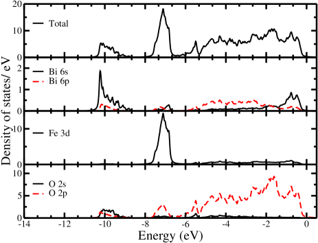
Figure 1: Total and projected density of states of BiFeO₃ in the valence band, calculated using the LSDA+U method with U= 6 eV and J= 0.9 eV. The top of the valence band is set to zero.

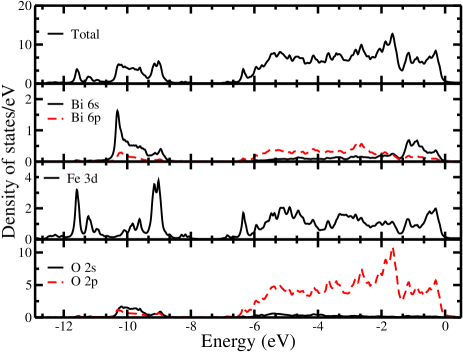
Figure 2: Total and projected density of states of BiFeO₃ in the valence band, calculated using the LDA+DMFT method with U= 6 eV and J= 0.9 eV. The top of the valence band is set to zero.

In FIGs.1 and 2, we present total and orbital-projected valence band density of states (DOSs) evaluated using LSDA+U and LDA+DMFT methods, respectively. Each figure contains total DOSs in the top panel and Bi 6$s$, Bi 6$p$, Fe 3$d$, O 2$s$ and O 2$p$ projected DOSs (PDOSs) in the lower panels. The PDOSs of Bi 5$d$, Fe 4$s$ and Fe 4$p$ are extremely small and featureless over the considered energy range and therefore, exempted from the following discussions.

A general inspection of the LSDA+U result (FIG. 1) indicates that the total DOSs from energy 0 eV to $\sim$-7 eV are caused by hybridization involving Fe, O and Bi states, which is consistent with previous reports. The Fe 3$d$ and O 2$p$ states interact strongly, whereas Bi 6$s$ and 6$p$ states couple weakly with the other two elements. The Bi states located around -10 eV predominantly have 6$s$ character and are attributed to stereochemically active lone-pairs. However, small amount of states from Bi 6$p$ and O 2$p$ orbitals are also found which compares well with the literatures. The DMFT result (FIG. 2) has several features that are similar to LSDA+U calculation, at least for Bi and O derived states. However, the spectral features of Fe 3$d$ states are markedly different, as can be seen by comparing FIGs.1 and 2. We will return to this discussion below, but first, we note that our calculated insulating gap using DMFT method in the PM phase is $\sim$1.22 eV, which tally well with Ref. Shorikov et al., 2015. The value of the energy gap once again confirms that it is independent of long-range magnetic order. The conduction band minimum (CBM) in both the methods is characterized by states from the upper Hubbard band of Fe 3$d$ orbitals (data not shown). The valence band maximum (VBM) has leading contribution from Fe 3$d$ and O 2$p$ bands and trivial one from Bi 6$s$ and 6$p$ bands.

Comparison of FIGs.1 and 2 shows that the total DOSs calculated from the two methods are markedly different. A detailed analysis reveals that the disagreement mainly occurs due to the differences in Fe 3$d$ DOSs. The LSDA+U method pushes most of the Fe 3$d$ electrons into a region of very narrow energy range which is visible from sharp and high DOSs at around -7 eV with small hybridization with Bi and O states. The prominent Fe peak in the LSDA+U result is replaced by multiplet features in the DMFT calculation and the spectral weight is distributed over wider energy intervals. The 3$d$ DOSs are found to be significant in energy intervals from the Fermi level down to -6.5 eV and from -8.5 to -12 eV (see FIG. 2). The Fe 3$d$ states closer to the Fermi level are characterized by significant hybridization with O 2$p$ and Bi 6$p$ states, while the Fe 3$d$ states from -8.5 to -12 eV are less hybridized. However, intensity of the multiplet peaks at lower energy interval is significant and curiously their position overlap with Bi 6$s$ lone-pairs. Hence, the result of FIG. 2 brings forth a picture where the Bi lone-pairs are not so lonely anymore and have significant spectral contribution from Fe 3$d$ multiplet structures around -10 eV. It is important to mention that, in our LDA+DMFT calculation, the electronic occupation of the Fe 3$d$ orbitals is 5.85, thus, referring to an electronic configuration closer to d⁶.

It is sufficient to compare the total DOSs and Fe 3$d$ PDOSs directly to measured HAXPES and RPES spectra, respectively, for demonstrating the superiority of the DMFT method and for interpretations of the measured spectra. However, for analyzing intricate details of the experimental spectra by comparing it to the theoretical results and thus, obtaining detailed understanding about the origin of all the spectral structures, one need to take the cross-section into account. We present such comparison and analysis in the next subsection.

III.2 Comparison between theoretical and experimental spectra and analysis of the spectral behavior

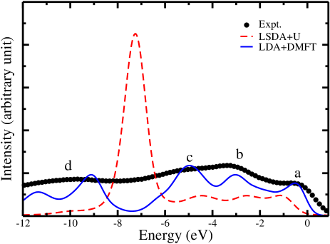
Figure 3: A comparison between the experimental RPES spectra (Ref. Mazumdar et al., 2016) and the theoretical spectra for Fe 3$d$ states of BiFeO₃ using LSDA+U and DMFT methods. The theoretical calculations are performed using U= 6 eV and J= 0.9 eV. The experimental data are shifted to align with the calculated valence band edge (see text).

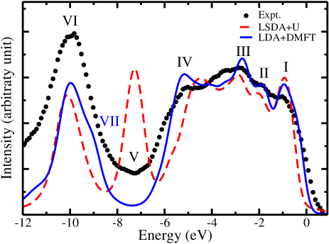
Figure 4: A comparison between the experimental HAXPES spectra (Ref. Mazumdar et al., 2016) and the theoretical spectra of BiFeO₃ using LSDA+U and DMFT methods. The theoretical calculations were performed using U= 6 eV and J= 0.9 eV. The experimental data are shifted to align with the calculated valence band edge (see text).

In FIGs.3 and 4, we compare the calculated Fe 3$d$ projected and total electronic spectra from LSDA+U and LDA+DMFT approaches to experimental RPES and HAXPES spectra, respectively Mazumdar et al. (2016). Note that in FIG. 4, cross-sections of all the valence states are taken into consideration. The experiment was performed at room temperature and HAXPES and RPES data were collected at photon energy of 2 keV and at photon energy corresponding to L₃ absorption peak of Fe, respectively. The latter photon energy produces resonant measurement that primarily signifies Fe 3$d$ states. It is noticeable in the experimental spectra published by Mazumdar et al. Mazumdar et al. (2016) that the position of the Fermi level is not located at the valence band maximum, which often is due to defects in the sample. To remove the ambiguity in Fermi level, we shifted the experimental spectra to match the valence band onset.

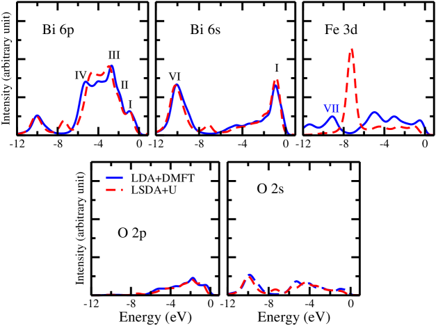
Figure 5: Atom and orbital projected spectral states of BiFeO₃ from LDA+U and DMFT methods. The calculations are done with Coulomb interaction parameters U= 6 eV and J= 0.9 eV. All the spectra are normalized in intensity with respect to the Bi 5$d$ state (data not shown).

In FIG. 3, the RPES spectra show a three-peak structure, denoted by $a$, $b$ and $c$, between 0 eV to -6 eV, where the third peak ($c$) is less conspicuous compared to the others. There is also a broad and weaker spectral contribution, denoted by $d$, that is centered around -10 eV. A general comparison illustrates that the LSDA+U result reproduces the experimental spectra with poor accuracy. The intensity of the spectra computed from LSDA+U method, in the energy range between 0 eV and -6 eV, is very small and shows marginal variations; then it rapidly enhanced to a sharp peak at around -7 eV and thenceforth, it vanishes quickly with further increase in binding energy. Overall, this does not represent the general features as captured in the experiment. The LSDA+U result generates a three-peak structures below -6 eV, as also found in the RPES spectra. However, the position and intensity of LSDA+U derived peaks do not coincide with the experimental result. Furthermore, the large peak at around -7 eV is entirely missing from the experimental observation. It is pellucid from the fact that the RPES spectra exhibit a dip in the intensity pattern at the position of that theoretical peak. The discrepancy also persists at higher binding energies, since no significant amount of Fe 3$d$ states are found in FIG. 1 that match the measured hump centered around -10 eV in the resonant spectra.

On the other hand, DMFT result conforms better with the RPES spectra regarding the positions of all the peaks and the width of the spectra. In theory, we found significant amount of intensity in the entire energy range in accordance with the experimental data. Note that measured intensity at binding energies higher than 12 eV is caused by secondary emission which forms a general background to the spectra. The intensity of the spectra for the DMFT method is found to increase gradually from peak $a$ to $c$, in agreement with the experiment. Also, non-negligible contribution to the spectra at higher binding energies up to 12 eV is perfectly captured by the theory and as discussed above this is due to 3$d$ multiplets at lower energy interval (see FIG. 2). The measured spectra in FIG. 3 have a small dip at around -7.5 eV, which is also present in the theory, albeit here the dip is more pronounced. Although the reason for this disagreement is a matter of debate, but we conclude that the overall features are well captured. The aforesaid discourse indicates that the correlation effects among the Fe 3$d$ electrons are important and properly considered within the DMFT calculation.

In FIG. 4, the valence band HAXPES spectra show a sharp peak near the Fermi level at -0.9 eV (feature I), followed by two more closely positioned peaks at -1.85 eV and -2.7 eV, denoted by features II and III, respectively. A distant fourth peak is located at -5.2 eV (feature IV), separated from peak III by a region having little variation in intensity. Furthermore, around -10 eV, we observe an extended crest (feature VI) succeed by a valley (feature V). A careful inspection shows that at low and high binding energies, both the theoretical methods generate similar results which are more or less consistent with the HAXPES spectra. However, in the intermediate and high binding energy range, the LSDA+U result deviates from experimental result significantly, whereas the DMFT result matches with the experimental spectra.

One a more detailed level, we note that the structures of our theoretical spectra for the two methods down to -3 eV match more or less well with the three peaks of the HAXPES data both in terms of position and intensity. Thereafter, the LSDA+U result starts to depart from the experimental data and hence, the first countable difference arises as the position of the fourth peak (IV) is underestimated by $\sim$0.7 eV in the spectra calculated using LSDA+U method, whereas the DMFT derived spectra better captures the characteristic of peak IV. The region with minimal variation between peak III and IV of the experimental spectra is nicely captured in the DMFT result, showing a smooth variation of intensity with energy. The second and most noticeable difference occurs due to the sharp peak in LSDA+U result, that is located around -7 eV. This originates, as discussed above, from the high intensity peak related to Fe 3$d$ states. In contrast to the LSDA+U result, we observe a valley in the DMFT spectra at that energy which is consistent with the measured HAXPES spectra. Around -10 eV, qualitatively both the theoretical methods produce a broad pattern in accordance with the HAXPES spectra, although discernible difference in intensity between theoretical and experimental spectra is observed. This difference is due to the fact that we do not include background signals in our calculation which is present in the experiment. We have chosen not to include the background since its absence does not alter our physical reasoning of different features in the spectra. The finer details of peak VI shows a weak structure in the HAXPES measurements that seem to be composed by two overlapping peaks (FIG. 4). This is not captured by the LSDA+U calculation that has a single smooth feature, nor by the DMFT calculation which has more structure compared to the previous method. However, the DMFT derived spectra exhibit a shoulder at feature VII, instead of two-peak structure.

In order to analyze the elemental contributions to the theoretical spectra, we present orbital projected states of Bi 6$s$, Bi 6$p$, Fe 3$d$, O 2$s$, and O 2$p$ in FIG. 5. Both the DMFT and the LSDA+U results are presented. Although the DOSs for Bi in FIG. 2 are small relative to Fe and O throughout the energy range, due to higher cross-section, the element has largest spectral weight and mostly decides the structures of the spectra. On the other hand, due to lower cross-section, the spectral intensity of Fe and O states have less significant contributions to the spectra. The first peak (I) has biggest contribution from Bi 6$s$ states and moderate amount of contribution from Bi 6$p$ states. From there on, the intensity of Bi 6$s$ states decreases promptly, becomes comparable to the intensity of Fe and O states and less important for features up to -6 eV. In contrast, the intensity of Bi 6$p$ states increase rapidly and dominate the intermediate peaks II, III and IV. The Fe 3$d$, O 2$s$ and O 2$p$ states offer a small weight to the spectra throughout the energy range. The extended feature VI is governed by Bi 6$s$ states but have influences from Bi 6$p$ and O 2$s$ states and from the DMFT calculations, also the Fe 3$d$ states. In all the figures, spectral characteristic computed using the LSDA+U method deviates slightly from the DMFT results, except for Fe 3$d$ states, where the difference is most significant. The spectral properties are mostly affected by the changes in Fe 3$d$ spectra and similarities near the two extreme energy limits are primarily controlled by Bi 6$s$ and Bi 6$p$ spectra.

IV Conclusion

In this paper, we resolve the discrepancies in the electronic excitation spectra of extensively investigated multiferroic BiFeO₃ between experiment and LSDA+U method with improved results from LDA+DMFT method. Our calculations demonstrate that an accurate description of the electronic correlation among the Fe 3$d$ electrons is necessary to obtain good agreement with the experiment. The LSDA+U method offers poor description of the electronic structure due to its limited treatment of correlation effects. For the two methods, we observe that the changes in DOSs are most prominent for Fe 3$d$ states, whereas it is trivial for the other two constituent elements. The high-intensity narrow peak in Fe 3$d$ DOSs obtained under LSDA+U method, redistributed under LDA+DMFT approach and generates multiplet structures that spread over wider energy regions. The Fe 3$d$ multiplets at lower energies appear at the position of Bi 6$s$ lone-pairs states, signifying hybridization between those orbitals, which is completely absent in LSDA+U picture. The reorganized Fe 3$d$ DOSs in LDA+DMFT method when multiplied with cross-section capture the features of the experimental RPES spectra, whereas the other method drastically fails to even produce the general features of the measured spectra. Similarly, on the overall energy range, the features produce by LDA+DMFT method agrees well with the experimental HAXPES measurement. Inspection of element resolved LDA+DMFT derived spectra reveals that Bi mostly governs the behavior of the spectra and the other two element have small contributions. The same investigation for the two theoretical methods illustrates that similarities in the spectra are due to Bi derived states and changes are caused by Fe 3$d$ states. Summarizing, we produce theoretical valence band spectra for BiFeO₃ with LDA+DMFT method which nicely matches with all the experimental features and shows that dynamical correlation is important for this multiferroic material.

Appendix A Influence of the interaction parameters on the spectra

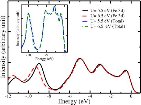
Figure 6: Theoretical spectra of Fe 3$d$ states calculated under LDA+DMFT method for two different U values, keeping J fixed to 0.9 eV. The inset shows total spectra for the same U values.

It is interesting to examine the impact of the Coulomb interaction parameter U on the spectra. For this, we have performed LDA+DMFT calculations for two different values of U, below and above 6 eV, with fixed J= 0.9 eV. In FIG. 6, we present total and Fe 3$d$ projected spectra of such calculations. On an overall basis, features in the total spectra remain static to the variation of Hubbard parameter U, whereas some changes are observed in the Fe 3$d$ spectra. The basic features of the two curves for Fe 3$d$ in FIG. 6 are similar to one in FIG. 3; however, features at higher binding energies move sightly away from the Fermi level when U is increased. The strong hybridization of Fe 3$d$ orbitals with the bath orbitals (O 2$p$) between 0 and -6 eV allows to overcome the effect of variation in U and consequently no changes are observed in the spectra. On the contrary, due to extremely low degree of hybridization, Fe 3$d$ states at higher binding energies behave close to atomic-like and result in the observed behavior. We observe minimal changes when all these spectra are compared with J= 1.0 eV, keeping U fixed (data not shown). From this discussion, we can conclude that the choices of interaction parameters do not alter the physical apprehension of the spectral properties in this material as long as their values are plausible.

Our calculated electronic spectra using DFMT method at photon energy of 6 keV differ significantly at higher binding energies in terms of intensity with the measured spectra in Ref. Mazumdar et al., 2016. Recently, with the aid of DMFT+GW calculations in NiO, Panda et al. Panda et al. (2016) showed that the effect of non-local correlation on the delocalized states is important to explain the structures of excitation spectra at high photon energy. Based on their observation, we come to the resolution that our local correlation based DMFT result is not sufficient to produce spectra at such high energy for BiFeO₃ and we leave the investigation by including non-local correlations within the calculations for future publication.

References

- Ramesh and Spaldin (2007) R. Ramesh and N. A. Spaldin, Nat Mater 6, 21 (2007).
- Schmid (1994) H. Schmid, Ferroelectrics 162, 317 (1994).
- Spaldin et al. (2010) N. A. Spaldin, S.-W. Cheong, and R. Ramesh, Phys. Today 63, 38 (2010).
- Wang et al. (2003) J. Wang, J. B. Neaton, H. Zheng, V. Nagarajan, S. B. Ogale, B. Liu, D. Viehland, V. Vaithyanathan, D. G. Schlom, U. V. Waghmare, N. A. Spaldin, K. M. Rabe, M. Wuttig, and R. Ramesh, Science 299, 1719 (2003).
- Moreau et al. (1971) J. Moreau, C. Michel, R. Gerson, and W. James, J. Phys. Chem. Solids 32, 1315 (1971).
- Michel et al. (1969) C. Michel, J.-M. Moreau, G. D. Achenbach, R. Gerson, and W. James, Solid State Commun. 7, 701 (1969).
- Neaton et al. (2005) J. B. Neaton, C. Ederer, U. V. Waghmare, N. A. Spaldin, and K. M. Rabe, Phys. Rev. B 71, 014113 (2005).
- Sosnowska et al. (1982) I. Sosnowska, T. P. Neumaier, and E. Steichele, J. Phys. C: Solid State Phys. 15, 4835 (1982).
- Zhang et al. (2005) S. T. Zhang, M. H. Lu, D. Wu, Y. F. Chen, and N. B. Ming, Appl. Phys. Lett. 87, 262907 (2005).
- Ederer and Spaldin (2005) C. Ederer and N. A. Spaldin, Phys. Rev. B 71, 060401 (2005).
- Kadomtseva et al. (2004) A. M. Kadomtseva, A. K. Zvezdin, Y. F. Popov, A. P. Pyatakov, and G. P. Vorob’ev, JETP. Lett. 79, 571 (2004).
- Popov et al. (1993) Y. F. Popov, A. K. Zvezdin, G. P. Vorob’ev, A. M. Kadomtseva, V. A. Murashev, and D. N. Rakov, JETP Lett. 57, 69 (1993).
- Popov et al. (1994) Y. F. Popov, A. M. Kadomtseva, G. P. Vorob’ev, and A. K. Zvezdin, Ferroelectrics 162, 135 (1994).
- Le Bras et al. (2009) G. Le Bras, D. Colson, A. Forget, N. Genand-Riondet, R. Tourbot, and P. Bonville, Phys. Rev. B 80, 134417 (2009).
- Bai et al. (2005) F. Bai, J. Wang, M. Wuttig, J. Li, N. Wang, A. P. Pyatakov, A. K. Zvezdin, L. E. Cross, and D. Viehland, Appl. Phys. Lett. 86, 032511 (2005).
- Baettig et al. (2005) P. Baettig, C. Ederer, and N. A. Spaldin, Phys. Rev. B 72, 214105 (2005).
- Clark and Robertson (2007) S. J. Clark and J. Robertson, Appl. Phys. Lett. 90, 132903 (2007).
- Shang et al. (2009) S. L. Shang, G. Sheng, Y. Wang, L. Q. Chen, and Z. K. Liu, Phys. Rev. B 80, 052102 (2009).
- Ju et al. (2009) S. Ju, T.-Y. Cai, and G.-Y. Guo, J. Chem. Phys. 130, 214708 (2009).
- Goffinet et al. (2009) M. Goffinet, P. Hermet, D. I. Bilc, and P. Ghosez, Phys. Rev. B 79, 014403 (2009).
- He et al. (2015) C. He, Z.-J. Ma, B.-Z. Sun, R.-J. Sa, and K. Wu, J. Alloys Compd. 623, 393 (2015).
- Yaakob et al. (2015) M. K. Yaakob, M. F. M. Taib, L. Lu, O. H. Hassan, and M. Z. A. Yahya, Mater. Res. Express 2, 116101 (2015).
- Mazumdar et al. (2016) D. Mazumdar, R. Knut, F. Thöle, M. Gorgoi, S. Faleev, O. Mryasov, V. Shelke, C. Ederer, N. Spaldin, A. Gupta, and O. Karis, J. Electron Spectrosc. Relat. Phenom. 208, 63 (2016), special Issue: Electronic structure and function from state-of-the-art spectroscopy and theory.
- Grånäs et al. (2012) O. Grånäs, I. D. Marco, P. Thunström, L. Nordström, O. Eriksson, T. Björkman, and J. Wills, Comput. Mater. Sci. 55, 295 (2012).
- Thunström et al. (2012) P. Thunström, I. Di Marco, and O. Eriksson, Phys. Rev. Lett. 109, 186401 (2012).
- Diéguez et al. (2011) O. Diéguez, O. E. González-Vázquez, J. C. Wojdeł, and J. Íñiguez, Phys. Rev. B 83, 094105 (2011).
- Georges et al. (1996) A. Georges, G. Kotliar, W. Krauth, and M. J. Rozenberg, Rev. Mod. Phys. 68, 13 (1996).
- Kotliar et al. (2006) G. Kotliar, S. Y. Savrasov, K. Haule, V. S. Oudovenko, O. Parcollet, and C. A. Marianetti, Rev. Mod. Phys. 78, 865 (2006).
- Held (2007) K. Held, Advances in Physics 56, 829 (2007).
- Anderson (1961) P. W. Anderson, Phys. Rev. 124, 41 (1961).
- Pavarini et al. (2004) E. Pavarini, S. Biermann, A. Poteryaev, A. I. Lichtenstein, A. Georges, and O. K. Andersen, Phys. Rev. Lett. 92, 176403 (2004).
- Pavarini et al. (2005) E. Pavarini, A. Yamasaki, J. Nuss, and O. K. Andersen, New Journal of Physics 7, 188 (2005).
- Solovyev (2008) I. V. Solovyev, Journal of Physics: Condensed Matter 20, 293201 (2008).
- De Raychaudhury et al. (2007) M. De Raychaudhury, E. Pavarini, and O. K. Andersen, Phys. Rev. Lett. 99, 126402 (2007).
- Nekrasov et al. (2005) I. A. Nekrasov, G. Keller, D. E. Kondakov, A. V. Kozhevnikov, T. Pruschke, K. Held, D. Vollhardt, and V. I. Anisimov, Phys. Rev. B 72, 155106 (2005).
- Ohta et al. (2012) K. Ohta, R. E. Cohen, K. Hirose, K. Haule, K. Shimizu, and Y. Ohishi, Phys. Rev. Lett. 108, 026403 (2012).
- Gorelov et al. (2010) E. Gorelov, M. Karolak, T. O. Wehling, F. Lechermann, A. I. Lichtenstein, and E. Pavarini, Phys. Rev. Lett. 104, 226401 (2010).
- Mravlje et al. (2011) J. Mravlje, M. Aichhorn, T. Miyake, K. Haule, G. Kotliar, and A. Georges, Phys. Rev. Lett. 106, 096401 (2011).
- Zhang et al. (2013) H. Zhang, K. Haule, and D. Vanderbilt, Phys. Rev. Lett. 111, 246402 (2013).
- Haule et al. (2014) K. Haule, T. Birol, and G. Kotliar, Phys. Rev. B 90, 075136 (2014).
- Dang et al. (2014) H. T. Dang, X. Ai, A. J. Millis, and C. A. Marianetti, Phys. Rev. B 90, 125114 (2014).
- Dang et al. (2015) H. T. Dang, J. Mravlje, A. Georges, and A. J. Millis, Phys. Rev. B 91, 195149 (2015).
- Shorikov et al. (2015) A. O. Shorikov, A. V. Lukoyanov, V. I. Anisimov, and S. Y. Savrasov, Phys. Rev. B 92, 035125 (2015).
- Kockelmann et al. (2001) W. A. Kockelmann, W. Schäfer, I. Sosnowska, and I. Troyanchuk, in European Powder Diffraction EPDIC 7, Mater. Sci. Forum, Vol. 378 (Trans Tech Publications, 2001) pp. 616–620.
- Dreysse (2000) H. Dreysse, ed., Electronic Structure and Physical Properties of Solids: The Uses of the LMTO Method (Springer Berlin Heidelberg, 2000).
- Wills et al. (2010) J. M. Wills, O. Eriksson, P. Andersson, A. Delin, O. Grechnyev, and M. Alouani, “Full-Potential Electronic Structure Method: Energy and Force Calculations with Density Functional and Dynamical Mean Field Theory,” (Springer Berlin Heidelberg, Berlin, Heidelberg, 2010).
- von Barth and Hedin (1972) U. von Barth and L. Hedin, J. Phys. C: Solid State Phys. 5, 1629 (1972).
- Hedin and Lundqvist (1971) L. Hedin and B. I. Lundqvist, J. Phys. C: Solid State Phys. 4, 2064 (1971).
- Anisimov et al. (1993) V. I. Anisimov, I. V. Solovyev, M. A. Korotin, M. T. Czyżyk, and G. A. Sawatzky, Phys. Rev. B 48, 16929 (1993).
- Caroli et al. (1973) C. Caroli, D. Lederer-Rozenblatt, B. Roulet, and D. Saint-James, Phys. Rev. B 8, 4552 (1973).
- Feibelman and Eastman (1974) P. J. Feibelman and D. E. Eastman, Phys. Rev. B 10, 4932 (1974).
- Marksteiner et al. (1986) P. Marksteiner, P. Weinberger, R. C. Albers, A. M. Boring, and G. Schadler, Phys. Rev. B 34, 6730 (1986).
- Panda et al. (2016) S. K. Panda, B. Pal, S. Mandal, M. Gorgoi, S. Das, I. Sarkar, W. Drube, W. Sun, I. Di Marco, A. Lindblad, P. Thunström, A. Delin, O. Karis, Y. O. Kvashnin, M. van Schilfgaarde, O. Eriksson, and D. D. Sarma, Phys. Rev. B 93, 235138 (2016).