The full Quantum Spectral Curve for AdS₄/CFT₃

Abstract

The spectrum of planar $\mathcal{N}=6$ superconformal Chern-Simons theory, dual to type IIA superstring theory on $AdS_{4}\times CP^{3}$, is accessible at finite coupling using integrability. Starting from the results of [arXiv:1403.1859], we study in depth the basic integrability structure underlying the spectral problem, the Quantum Spectral Curve. The new results presented in this paper open the way to the quantitative study of the spectrum for arbitrary operators at finite coupling. Besides, we show that the Quantum Spectral Curve is embedded into a novel kind of Q-system, which reflects the $OSp(4|6)$ symmetry of the theory and leads to exact Bethe Ansatz equations. The discovery of this algebraic structure, more intricate than the one appearing in the $AdS_{5}/CFT_{4}$ case, could be a first step towards the extension of the method to $AdS_{3}/CFT_{2}$.

1 Introduction

The idea of a duality between gauge and string theory was put forward many years ago by ’t Hooft tHooft:1973alw , who noticed that the perturbative expansion in $SU(N_{c})$ Yang-Mills theory in the large $N_{c}$ limit naturally organizes in terms of the topology of Feynman diagrams, mimicking the genus expansion of string theory.

The first concrete realization of the duality Maldacena:1997re ; Gubser:1998bc ; Witten:1998qj conjectures the exact equivalence of $\mathcal{N}=4$ super Yang-Mills (SYM) theory and type IIB string theory on $AdS_{5}\times S^{5}$. The precise identification of observables and parameters in the two theories relates the perturbative region of each model to the deep non-perturbative regime of the other. For this reason, the correspondence makes powerful predictions, but is also very difficult to test.

An important turning point in this field was the discovery of fingerprints of integrability, at both weak and strong coupling MZ ; Bena:2003wd , in the planar limit of this duality. At least in this limit, it is hoped that the theory will be exactly solved adapting integrable model tools, and remarkable progress has been made on the study of various observables, including Wilson loops and correlation functions.

In particular, the problem of computing the conformal spectrum of the theory was tackled by tailoring integrable QFT techniques to this new setting, in particular the Bethe Ansatz MZ ; Beisert:2005fw ; Beisert:2006ez , the TBA, the Y and T-systems BFT ; AF ; GKKV ; Extended ; Balog:2011nm ; Wronskian ; FiNLIE , leading to the discovery of the very effective Quantum Spectral Curve (QSC) formulation QSC ; Gromov:2014caa . The latter is a very satisfactory simplification and probably the most elementary formulation of the problem. Thanks to the mathematical simplicity of the QSC, it appears that, in the near future, the spectral problem may be completely solved also in a practical/computational sense. Already, the QSC method allows to compute the spectrum numerically with high precision Gromov:2015wca ; Hegedus:2016eop and to inspect analytically interesting regimes such as the BFKL limit QCDPomeron ; Gromov:2015vua or the weak coupling expansion Marboe:2014gma ; MarboeTalk ; Marboe:2017dmb . It has also been generalized to so-called $\gamma$ deformations Thook and to the quark-antiquark potential QSCCusp ; QSCPotential .

Another remarkable example of AdS/CFT correspondence was introduced by Aharony, Bergman, Jafferis and Maldacena (ABJM) in Aharony:2008ug . The gauge side of the duality corresponds to the $\mathcal{N}=6$ superconformal Chern-Simons theory with gauge group $U(N)\times U(N)$, with opposite Chern-Simons levels, $k$ and $-k$, for the two $U(N)$ factors. We will be concerned with the planar limit, where $k,N\rightarrow\infty$ with the ’t Hooft coupling $\lambda=\frac{k}{N}$ kept finite and the dual gravity theory becomes type IIA superstring theory on $AdS_{4}\times CP^{3}$. In this regime, integrability emerges, making the ABJM model the only known example of 3d quantum field theory which can be exactly solved Minahan:2008hf ; Gaiotto:2008cg ; Stefanski:2008ik ; Arutyunov:2008if ; Gromov:2008bz (see also the review Klose:2010ki ).

The spectral problem in ABJM theory was approached exploiting the experience gained in $AdS_{5}/CFT_{4}$. Anomalous dimensions of single trace operators with asymptotically large quantum numbers are described at all loop by the so-called Asymptotic Bethe Ansatz equations, conjectured in Gromov:2008qe and derived from the exact worldsheet S-matrix of Ahn:2008aa . The exact result, including all finite-size corrections for short operators, is formally described by an infinite set of TBA equations, proposed in Bombardelli:2009xz ; Gromov:2009at . These equations were solved numerically for a particular operator in LevkovichMaslyuk:2011ty . However, solving excited states TBA equations with high precision is a challenging task already for very simple models DT ; Bazhanov:1996aq ; DoreyPerturbedCFT . Besides, the form of the TBA equations depends on the state and possibly also on the range of the coupling considered, so that they can be studied only on a case-by-case basis.

It is important to look for a simpler formulation which overcomes these problems. Starting from a precise knowledge of the analytic properties of the TBA solutions ABJMdisco , the basic equations characterizing the Quantum Spectral Curve of the ABJM model were obtained in Cavaglia:2014exa . These results were used to compute the so-called slope function in a near-BPS finite coupling regime Gromov:2014eha and to develop a generic algorithm for the weak coupling expansion in the $SL(2)$-like sector Anselmetti:2015mda .

Although we stress that, as proved by the applications discussed above, the results of Cavaglia:2014exa contain all the analytic information necessary to solve the spectral problem, several important aspects of the full picture were still missing. First of all, the concrete recipe to describe states within the QSC framework was discussed in Cavaglia:2014exa only for the $SL(2)$-like sector. Secondly, the set of equations obtained in Cavaglia:2014exa , the ${\bf P}\mu$/${\bf P}\nu$-system, can be associated, in the classical limit, to degrees of freedom related to the $CP^{3}$ part of the whole $AdS_{4}\times CP^{3}$ target space. A dual system of equations, only briefly mentioned in Cavaglia:2014exa , may be instead associated to $AdS_{4}$ classical degrees of freedom. The interplay between the two systems is important for the development of the state-of-the-art solution algorithm at finite coupling Gromov:2015wca , as well as at weak coupling for generic states Gromov:2015vua ; MarboeTalk . Furthermore, the full algebraic structure was still not transparent, and for example the link between the formulation of Cavaglia:2014exa and the Asymptotic Bethe Ansatz of Gromov:2008qe was difficult to see. In this paper we will fill these gaps and present the necessary elements for the quantitative solution of the spectral problem for an arbitrary operator at finite coupling. Besides, we reveal an interesting underlying representation theory structure, which could allow for generalizations and may in particular help in the solution of the spectral problem for $AdS_{3}/CFT_{2}$ dualities (see SfondriniReview for a recent review).

To conclude this introduction, let us review an important fact. In contrast with $\mathcal{N}$=4 SYM, in ABJM theory integrability leaves unfixed the so-called interpolating function $h(\lambda)$ Gaiotto:2008cg ; Grignani:2008is , which parametrizes the dispersion relation of elementary spin chain/worldsheet excitations and enters as an effective coupling constant in the integrability-based approach, in particular in the QSC equations. An important conjecture for the exact form of this function, passing several tests at weak and strong coupling Bianchi:2014ada , was made in Gromov:2014eha by a comparison with the structure of localization results. This conjecture was extendend in Cavaglia:2016ide to encompass the ABJ model Aharony:2008gk , which is based on a more general gauge group $U(N)\times U(M)$ and possesses two ’t Hooft couplings $\lambda_{1}$, $\lambda_{2}$ in the planar limit. According to the proposal of Cavaglia:2016ide (based on important observations of Bak:2008vd ; Minahan:2009te ; Minahan:2010nn ; Bianchi:2016rub ), at the level of the spectrum the only difference between the ABJM and ABJ theories lies in the replacement of $h(\lambda)$ with an explicitly defined $h^{\text{ABJ}}(\lambda_{1},\lambda_{2})$ (see Cavaglia:2016ide ). In the following we will simply denote the ABJM/ABJ interpolating function as $h$.

The contents of this paper are presented in detail below.

In Section 2, we discuss the bosonic symmetry underlying the problem, namely $SO(3,2)\times SO(6)$, the isometry group of $AdS_{4}\times CP^{3}$. We will introduce important vector and spinor notation used in the rest of the paper. Besides, we comment on the interesting fact that the isometry group of $CP^{3}$ effectively appears in the Quantum Spectral Curve as $SO(3,3)$, rather than $SO(6)$.

In Section 3, we review the results of Cavaglia:2014exa and discuss how they reflect the $CP^{3}$ symmetry. We discuss a subtle modification of the analytic properties (initially overlooked in Cavaglia:2014exa ), which is needed for the study of certain non-symmetric sectors of the theory. The modified equations contain an extra nontrivial function of the coupling, which can be interpreted at weak coupling as the momentum of a single species of magnons.

In Section 4, we present an explicit construction of new variables, the functions ${\bf Q}_{I}$, ${\bf Q}_{\circ}$ and $\tau_{i}$, which satisfy a dual system of Riemann-Hilbert equations reflecting the symmetry of $AdS_{4}$.

In Section 5, we treat in full generality the boundary conditions which need to be imposed on the solutions of the QSC at large value of the spectral parameter in order to describe a physical state. This is the place where the quantum numbers of the state make an appearance. We also discuss the correspondence between the functions ${\bf P}$ and ${\bf Q}$ and quasi-momenta of the spectral curve in the classical limit.

In Section 6, based on results obtained in Gromov:2015vua ; ContiNumerical , we discuss a set of exact relations which are perhaps the most convenient way to repack the analytic properties discussed in Sections 3, 4. It is also shown how these equations encode the quantization of the spin.

In Section 7, we embed the previous results into a larger set of functional relations which may be considered as (part of) a Q-system. Q-systems are familiar in the theory of integrable models Krichever:1996qd ; Pronko:1999gh and in the ODE/IM framework Dorey:2006an : they are powerful sets of functional relations that, supplemented by simple analytic requirements, become equivalent to exact Bethe equations. The structure of Q-systems is completely fixed by symmetry: for example, the QQ relations appearing in the $\mathcal{N}$=4 SYM case are the same as the ones for $SU(4|4)$ spin chains. For the $OSp(4|6)$ superalgebra relevant to ABJM theory, however, this algebraic construction was not known in the literature. While we do not treat in full generality the representation theory aspects, we construct explicitly an enlarged set of Q functions, and prove that they satisfy exact Bethe equations reflecting the full supergroup structure. Generalizing arguments of Gromov:2014caa , we will show that, in the limit of large volume, some of these exact Bethe equations reduce to the Asymptotic Bethe Ansatz.

The paper also contains five Appendices:

In Appendix A, we discuss the details of the derivation (already summarized in Cavaglia:2014exa ) of the QSC from the analytic properties of the T-system ABJMdisco . In Appendix B, we list some useful algebraic identities used in the derivation of the Q-system relations. In Appendix C, we deduce some of the constraints on the asymptotics of ${\bf P}$ and ${\bf Q}$ functions. In Appendix D, we discuss the weak coupling limit of the QSC and show the emergence of the 2-loop Bethe equations of MZ . We exploit this link to prove the identification between the parameters entering the asymptotics of the QSC and the quantum numbers. Finally, in Appendix E we review the dictionary between $OSp(4|6)$ quantum numbers and number of Bethe roots appearing in various versions of the (Asymptotic) Bethe Ansatz, which could be useful for the reader wanting to apply the prescription of Section 5 to concrete states.

2 Symmetries and conventions

ABJM theory is invariant under the supergroup $OSp(4|6)$, whose bosonic subgroups are associated to the isometries of $AdS_{4}$ and $CP^{3}$. We will see that the Quantum Spectral Curve equations encode elegantly this symmetry structure. Let us briefly introduce the main group-theoretic constructions related to the bosonic symmetries.

• $CP^{3}$: the isometry group of $CP^{3}$ is the orthogonal group $SO(6)\simeq SU(4)$. The invariant $6\times 6$ symmetric tensor naturally associated to this symmetry is the metric. This tensor enters the QSC equations, and will be denoted in this paper as $\eta_{AB}$. Peculiarly, we will see that it appears in the QSC with a $(+++---)$ signature. The concrete form of $\eta_{AB}$ to be used in the rest of this paper is

  $$\eta_{AB}=\eta^{AB}=\left(\begin{array}[]{cccccc}0&0&0&1&0&0\\ 0&0&-1&0&0&0\\ 0&-1&0&0&0&0\\ 1&0&0&0&0&0\\ 0&0&0&0&0&1\\ 0&0&0&0&1&0\end{array}\right),$$ (1)

  where $\eta^{AB}$ is the inverse matrix, i.e. $\eta_{AB}\,\eta^{BC}=\delta_{A}^{C}$. This particular choice for $\eta_{AB}$ emerged naturally from the derivation of the QSC, summarized in Appendix A. As explained there, the specific form of $\eta_{AB}$ in (1) is partly conventional, but its signature cannot be modified without spoiling the reality properties of the system. The fact that the $CP^{3}$ symmetry appears effectively as $SO(3,3)$ can be understood heuristically considering the classical limit, where the basic variables of the QSC are related to the quasi-momenta of the algebraic curve (see Section 5.2). The quasi-momenta describing a string moving in $CP^{3}$ are defined through the diagonalization of a $SO(6)$ block of the classical monodromy matrix. An $SO(2n)$ orthogonal matrix in general cannot be diagonalized with a real transformation, so that the signature of the metric is not preserved in the eigenvectors basis; moreover, the signature changes precisely to the one typical of $SO(n,n)$.

  Let us introduce some conventions. We will use different index labels for objects with different symmetry properties. The indices $A,B,C=1,\dots,6$ will be assumed to carry the vector representation of $SO(3,3)$, and will always be lowered and raised with the metric $\eta_{AB}$ and its inverse $\eta^{AB}$, respectively. It will be useful to consider also spinor representations of $SO(3,3)$. The relevant $8\times 8$ gamma matrices are defined by

  $$\left\{\Gamma_{8\times 8}^{A},\Gamma_{8\times 8}^{B}\right\}=\eta^{AB}\,\text{Id}_{8\times 8}.$$ (2)

  In even dimensions, gamma matrices can always be written in a chiral form:

  $$\Gamma^{A}=\left(\begin{array}[]{c c }0&\sigma^{A}_{ab}\\ {(\bar{\sigma}^{A})}^{ab}&0\end{array}\right),$$ (3)

  where the matrices $\sigma^{A}_{ab}$ and ${(\bar{\sigma}^{A})}^{ab}$ satisfy

  $$\sigma^{A}_{ab}\,(\bar{\sigma}^{B})^{bc}+\sigma^{B}_{ab}\,(\bar{\sigma}^{A})^{bc}=\eta^{AB}\,\delta_{a}^{c}.$$ (4)

  While all our equations will be covariant, it is convenient to specify a concrete basis. The matrices $\sigma^{A}_{ab}$ and ${(\bar{\sigma}^{A})}^{ab}$ are defined in our conventions by

  $$V_{A}\sigma^{A}_{ab}=\left(\begin{array}[]{cccc}0&-V_{1}&-V_{2}&-V_{5}\\ V_{1}&0&-V_{6}&-V_{3}\\ V_{2}&V_{6}&0&-V_{4}\\ V_{5}&V_{3}&V_{4}&0\end{array}\right),\;\;\;\;V_{A}{({\bar{\sigma}}^{A})}^{ab}=\left(\begin{array}[]{cccc}0&V_{4}&-V_{3}&V_{6}\\ -V_{4}&0&V_{5}&-V_{2}\\ V_{3}&-V_{5}&0&V_{1}\\ -V_{6}&V_{2}&-V_{1}&0\end{array}\right),$$ (5)

  for an arbitrary vector $(V_{1},\dots,V_{6})$. Lower-case indices $a,b,c$ will always be taken to run over $1,\dots,4$ and will be reserved for the spinor representations. Note that there is a distinction between upper and lower spinor indices, as they belong to the chiral and anti-chiral spinor representations, respectively, which are equivalent to the representations $\bf{4}$ and $\bar{\bf{4}}$ of $SU(4)\simeq SO(6)$. Another natural tensor that will make an appearance in the equations is the anti-symmetrized product of gamma matrices,

  $$(\sigma^{AB})_{a}^{\;b}\equiv-\frac{1}{2}\left((\sigma^{A})_{ac}{({\bar{\sigma}}^{B})}^{cb}-(\sigma^{B})_{ac}{({\bar{\sigma}}^{A})}^{cb}\right).$$ (6)

• $AdS_{4}$: the isometry group of $AdS_{4}$ is $SO(3,2)\simeq Sp(4)$. We will denote the metric of this orthogonal group as $\rho_{IJ}$, and our concrete choice will be:

  $$\rho_{IJ}=\left(\begin{array}[]{cccccc}0&0&0&1&0\\ 0&0&-1&0&0\\ 0&-1&0&0&0\\ 1&0&0&0&0\\ 0&0&0&0&\frac{1}{2}\end{array}\right),\;\;\;\;\rho^{IJ}\equiv(\rho^{-1})^{IJ}=\left(\begin{array}[]{cccccc}0&0&0&1&0\\ 0&0&-1&0&0\\ 0&-1&0&0&0\\ 1&0&0&0&0\\ 0&0&0&0&2\end{array}\right).$$ (7)

  In the following, we shall always reserve the indices $I,J,K$, running over $1,\dots,5$, for the vector representation of $SO(3,2)$.

  Let us remind the reader of the isomorphism between $SO(3,2)$ and $Sp(4)$, the group of linear maps preserving a $4\times 4$ anti-symmetric two-form. One way to see this is to view $SO(3,2)$ as obtained from $SO(3,3)$ by reducing to the subspace orthogonal to a preferred vector $v$, with $v\cdot v=-1$.

  Then we see that an anti-symmetric two-form naturally emerges: $\kappa_{ij}\equiv v_{A}\,(\sigma^{A})_{ij}$. Let us denote a projection of the $\sigma$, $\bar{\sigma}$ matrices on the subspace orthogonal to $v$ as $\Sigma_{I}$, $\bar{\Sigma}_{I}$, respectively, with $I=1,\dots,5$. By construction, they satisfy the intertwining relations $\bar{\Sigma}_{I}^{ij}=\kappa^{ii_{1}}\,(\Sigma_{I})_{i_{1}i_{2}}\,\kappa^{i_{2}j}$, showing that there are in fact only five independent matrices $\Sigma_{I}$. The latter give a four dimensional representation of Clifford algebra:

  $$\left\{\Gamma_{4\times 4}^{I},\Gamma_{4\times 4}^{J}\right\}=\rho^{IJ}\,\text{Id}_{4\times 4},$$ (8)

  with

  $$(\Gamma_{4\times 4}^{I})_{i}^{j}\equiv(\Sigma^{I})_{ik}\,\kappa^{kj}=\kappa_{ij}(\bar{\Sigma}^{I})^{jk}.$$ (9)

  In the following, we will use indices $i,j,k,l$, running over $1,\dots,4$, to refer to the four-dimensional representation of $SO(3,2)$. Finally, one can introduce the anti-symmetric combinations

  $$(\bar{\Sigma}^{IJ})_{i}^{\;j}\equiv-\frac{1}{2}\left((\Sigma^{I})_{ik}{({\bar{\Sigma}}^{J})}^{kj}-(\Sigma^{J})_{ik}{({\bar{\Sigma}}^{I})}^{kj}\right),$$ (10)

  which play the role of generators of $SO(3,2)$. By construction, these generators leave invariant the two-form $\kappa_{ij}$: therefore the spinor representation of $SO(3,2)$ is identified with the fundamental representation of $Sp(4)$.

  In our concrete case, we see that the metric (7) is obtained from (1) by restricting to the subspace orthogonal to $v=(0,0,0,0,-1,1)$. Our choice for the $\Sigma$ matrices will be

  $$\Sigma^{I}\equiv\left(\sigma^{1},\sigma^{2},\sigma^{3},\sigma^{4},\sigma^{5}+\sigma^{6}\right),\;\;\;\;\;\;\;\bar{\Sigma}^{I}\equiv\left(\bar{\sigma}^{1},\bar{\sigma}^{2},\bar{\sigma}^{3},\bar{\sigma}^{4},\bar{\sigma}^{5}+\bar{\sigma}^{6}\right),$$ (11)

  and the two-form $\kappa_{ij}$ reads

  $$\kappa_{ij}\equiv v_{A}\,(\sigma^{A})_{ij}=\left(\begin{array}[]{cccc}0&0&0&1\\ 0&0&-1&0\\ 0&1&0&0\\ -1&0&0&0\end{array}\right).$$ (12)

3 Formulation of the QSC from the TBA

In this Section, we recall the first version of the QSC equations proposed in Cavaglia:2014exa . These equations were obtained through a reduction of the T-system, supplemented by analyticity properties extracted from the TBA Extended ; Cavaglia:2014exa , and ultimately take the form of a nonlinear Riemann-Hilbert problem defined on the complex domain of the spectral parameter $u$. In the $u$-plane, the Q functions have a characteristic pattern of branch points, whose positions depends on the coupling constant $h$ as specified below. These branch points will all be of square-root type. This peculiar kind of analytic structure for the Q functions, beside $AdS_{5}/CFT_{4}$, is also characteristic of some non-relativistic integrable systems such as the Hubbard model Cavaglia:2015nta . The derivation of the QSC equations is discussed in Appendix A.

3.1 Equations in vector form and analyticity conditions

In the first version of the equations derived from TBA, the basic variables are: six functions $\left\{{\bf P}_{A}(u)\right\}_{A=1}^{6}$, and a $6\times 6$ anti-symmetric matrix $\left\{\mu_{AB}(u)=-\mu_{BA}(u)\right\}_{A,B=1}^{6}$. They are constrained by the following quadratic conditions:

$${\bf P}_{5}{\bf P}_{6}-{\bf P}_{2}{\bf P}_{3}+{\bf P}_{1}{\bf P}_{4}=1,\quad\quad\quad\mu_{AB}\,\eta^{BC}\,\mu_{CD}\,=0,$$ (13)

where $\eta^{AB}$ is defined in (1). All these functions live on an infinite-sheet cover of the $u$-plane, which, however, is built out of a simple set of rules. On what we will consider the first Riemann sheet, the functions ${\bf P}_{A}(u)$ have a single branch cut, running from $-2h$ to $+2h$, see Figure 2. We assume that they have power-like asymptotics at large $u$, which means that they can be written as a Laurent series in the Zhukovsky variable $x(u)$:

$${\bf P}_{A}(u)=(x(u))^{-M_{A}}\,\sum_{n=0}^{\infty}\frac{c_{A,n}}{x^{n}(u)},\quad\quad\quad x(u)=\frac{\left(u+\sqrt{u-2h}\sqrt{u+2h}\right)}{2h}.$$ (14)

The functions $\mu_{AB}(u)$ instead display an infinite ladder of branch cuts, at $u\in(-2h\,,\,+2\,h)+i\mathbb{Z}$. They however have the following analyticity property (mirror periodicity):

$$\widetilde{\mu}_{AB}(u)=\mu_{AB}(u+i),$$ (15)

where the symbol tilde is used throughout the paper to denote analytic continuation around any of the branch points at $\pm 2h$ (see Figure 2), while the shift on the rhs is evaluated avoiding all branch cuts.

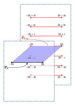
Figure 1: Cut structure of the ${\bf P}_{A}$ functions, with a single cut on the first sheet. We denote with $\widetilde{\bf P}_{A}$ the analytic continuation to the next sheet, through the cut on the real axis.

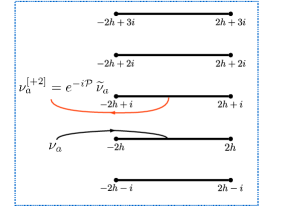
Figure 2: The quasi-periodicity property of $\nu_{a}$ functions on a sheet with long cuts corresponds to $\nu_{a}(u+i)=e^{-i\mathcal{P}}\,\widetilde{\nu}_{a}(u)$ on the defining sheet with short cuts.

Finally, the discontinuities of ${\bf P}_{A}$ and $\mu_{AB}$ across the cut on the real $u$-axis are related by

$${\widetilde{\bf P}}_{A}-{\bf P}_{A}=\mu_{AB}\,\eta^{BC}\,{\bf P}_{C},\;\;\;\;\;{\widetilde{\mu}}_{AB}-\mu_{AB}={\bf P}_{A}\widetilde{\bf P}_{B}-{\bf P}_{B}\widetilde{\bf P}_{A}.$$ (16)

In addition, as common for the Q functions in integrable models, we should impose a regularity condition for the basic variables ${\bf P}_{A}$ and $\mu_{AB}$. The precise statement of this condition, however, cannot be formulated in terms of the matrix entries $\mu_{AB}$, but of more fundamental building blocks which we introduce below.

3.2 Equations in spinor form

As already discussed in Cavaglia:2014exa , the matrix $\mu_{AB}$ can be decomposed in terms of $4+4$ functions $\nu_{a}$, $\nu^{a}$, as

$$\mu_{AB}=\left(\begin{array}[]{cccccc}0&\nu_{1}\nu^{4}&-\nu_{2}\nu^{3}&-\nu^{3}\nu_{3}-\nu^{4}\nu_{4}&-\nu_{1}\nu^{3}&\nu^{4}\nu_{2}\\ -\nu_{1}\nu^{4}&0&-\nu^{3}\nu_{3}-\nu_{1}\nu^{1}&\nu_{3}\nu^{2}&\nu_{1}\nu^{2}&\nu^{4}\nu_{3}\\ \nu_{2}\nu^{3}&\nu^{3}\nu_{3}+\nu_{1}\nu^{1}&0&-\nu_{4}\nu^{1}&\nu^{3}\nu_{4}&\nu_{2}\nu^{1}\\ \nu^{3}\nu_{3}+\nu^{4}\nu_{4}&-\nu_{3}\nu^{2}&\nu_{4}\nu^{1}&0&-\nu^{2}\nu_{4}&\nu_{3}\nu^{1}\\ \nu_{1}\nu^{3}&-\nu_{1}\nu^{2}&-\nu^{3}\nu_{4}&\nu^{2}\nu_{4}&0&-\nu^{3}\nu_{3}-\nu_{2}\nu^{2}\\ -\nu^{4}\nu_{2}&-\nu^{4}\nu_{3}&-\nu_{2}\nu^{1}&-\nu_{3}\nu^{1}&\nu_{2}\nu^{2}+\nu^{3}\nu_{3}&0\end{array}\right),$$ (17)

which, using the sigma matrices introduced in Section 2, can be compactly written as

$$\mu_{AB}=\nu^{a}\;(\sigma_{AB})_{a}^{\;b}\;\nu_{b}.$$ (18)

The constraint $(\mu\eta)^{2}=0$ is now equivalent to the condition

$$\nu^{a}\,\nu_{a}=0.$$ (19)

Motivated by the weak coupling analysis of Cavaglia:2014exa ; Anselmetti:2015mda , we will impose that the functions $\nu_{a}$, $\nu^{a}$ are analytic on any sheet of the Riemann surface, with the exception of the square-root branch points at $u\in i\mathbb{Z}\pm 2h$, and that they remain bounded as these points are approached. Besides, for physical values of the charges we assume that $\nu_{a}(u)$, $\nu^{a}(u)$ exhibit power-like asymptotics for $u\rightarrow\infty$. Under these conditions, the splitting (18) contains nontrivial analytic information, and may be argued to be essentially unique. The new functions $\nu_{a}$ and $\nu^{a}$ should therefore be regarded as more fundamental objects than $\mu_{AB}$. Indeed, at weak coupling, $\nu_{1}$ and $\nu^{4}$ are proportional to the Baxter polynomials containing the two types of momentum-carrying roots entering the 2-loop Bethe Ansatz of Minahan:2008hf , see Appendix D.1.

The weak coupling analysis also reveals that the periodicity of $\mu_{AB}$ on the mirror sheet, equation (15), in general translates into quasi-periodicity for the basic functions $\nu_{a}$, $\nu^{a}$ (see Figure 2). In the subsector considered in Anselmetti:2015mda , these functions could be either periodic or anti-periodic, and this is a general feature of a large sector of states discussed in Section 4.4. For a completely generic state, however, we have

$${\widetilde{\nu}}_{a}(u)=e^{i\mathcal{P}}\,\nu_{a}(u+i),\;\;\;\;\;{\widetilde{\nu}}^{a}(u)=e^{-i\mathcal{P}}\,\nu^{a}(u+i),$$ (20)

where the phase $\mathcal{P}$ depends on the state under consideration and may be, in general, a nontrivial function of the coupling constant $h$. We will make more comments on this quantity in Section 3.3 below.

It is now convenient to pack the six ${\bf P}$ functions into an anti-symmetric $4\times 4$ tensor ${\bf P}_{ab}$, defined as

$${\bf P}_{ab}={\bf P}_{A}\sigma^{A}_{ab}=\left(\begin{array}[]{cccc}0&-{\bf P}_{1}&-{\bf P}_{2}&-{\bf P}_{5}\\ {\bf P}_{1}&0&-{\bf P}_{6}&-{\bf P}_{3}\\ {\bf P}_{2}&{\bf P}_{6}&0&-{\bf P}_{4}\\ {\bf P}_{5}&{\bf P}_{3}&{\bf P}_{4}&0\end{array}\right),$$ (25)

while the inverse matrix reads

$${\bf P}^{ab}={\bf P}_{A}{({\bar{\sigma}}^{A})}^{ab} = \left(\begin{array}[]{cccc}0&{\bf P}_{4}&-{\bf P}_{3}&{\bf P}_{6}\\ -{\bf P}_{4}&0&{\bf P}_{5}&-{\bf P}_{2}\\ {\bf P}_{3}&-{\bf P}_{5}&0&{\bf P}_{1}\\ -{\bf P}_{6}&{\bf P}_{2}&-{\bf P}_{1}&0\end{array}\right).$$ (30)

The constraint (13) can now be rewritten as the condition that ${\bf P}_{ab}$ has unit Pfaffian:

$$\text{Pf}({\bf P}_{ab})=1.$$ (31)

Besides, it is possible to verify that the discontinuity equations (16) can be split nicely as

$${\widetilde{{\bf P}}}_{ab}-{\bf P}_{ab} = \nu_{a}{\tilde{\nu}}_{b}-\nu_{b}{\tilde{\nu}}_{a},\;\;\;\;\;{\widetilde{{\bf P}}}^{ab}-{\bf P}^{ab}=-\nu^{a}{\tilde{\nu}}^{b}+\nu^{b}{\tilde{\nu}}^{a},$$ (32)

$${\tilde{\nu}}_{a} = -{\bf P}_{ab}\;\nu^{b},\;\;\;\;\;{\tilde{\nu}}^{a}=-{\bf P}^{ab}\;\nu_{b}.$$ (33)

As discussed in Cavaglia:2014exa , in this form the equations are, from a purely algebraic point of view, exactly the same as the ${\bf P}\mu$-system of $\mathcal{N}=4$ SYM QSC ; Gromov:2014caa , with the redefinitions

$$\nu_{a}\rightarrow({\bf P}_{a})^{\text{SYM}},\;\;\;\;\;\nu^{a}\rightarrow({\bf P}^{a})^{\text{SYM}},\;\;\;\;\;{\bf P}_{ab}\rightarrow(\mu_{ab})^{\text{SYM}}.$$ (34)

The analytic properties characterizing the $AdS_{5}/CFT_{4}$ case are however completely different: the map between the two models in (34) requires to change all periodic functions into single-cut functions, and viceversa.

Equations (19),(31),(32) and (33) should be supplemented with the requirement that all functions are bounded and free of singularities on every sheet of the Riemann surface, and with some information on their large-$u$ asymptotics, see Section 5. This set of conditions is in principle already constraining enough to determine the spectrum, but it is difficult if not impossible to solve in practice at finite coupling. For this purpose it is necessary to embed them in the wider set of equations derived in Sections 4 and 6.

3.3 Interpretation of the phase $\mathcal{P}$ at weak coupling

The phase $\mathcal{P}$ appearing in (20) has an interesting interpretation at weak coupling. Recall that the ABJM spin chain admits two types of momentum-carrying excitations Aharony:2008ug ; Ahn:2008aa , also known as A and B particles and corresponding to excitations of type $4$ and $\bar{4}$ in our notations. These pseudoparticles satisfy collectively the zero momentum condition:

$$\sum_{j=1}^{K_{4}}p_{4,j}+\sum_{j=1}^{K_{\bar{4}}}p_{\bar{4},j}=0,\;\;\;\;\text{mod}(2\pi).$$ (35)

The total momentum of a single type of excitations is instead in general a nontrivial function of the coupling: it can be defined in the regime of validity of the Asymptotic Bethe Ansatz as

$$P^{({4})}_{\text{ABA}}=-P^{(\bar{{4}})}_{\text{ABA}}=\sum_{j=1}^{K_{4}}p_{4,j}=-\sum_{j=1}^{K_{\bar{4}}}p_{\bar{4},j},\;\;\;\;\text{mod}(2\pi),$$ (36)

where

$$p_{\mathit{s},j}=-i\log(x_{\mathit{s},j}^{+}/x_{\mathit{s},j}^{-}),\;\;\;\;x_{\mathit{s},j}^{\pm}=x(u_{\mathit{s},j}\pm i/2),\;\;\mathit{s}=4,\bar{4},$$ (37)

and $\left\{u_{4,j}\right\}_{j=1}^{K_{4}}$, $\left\{u_{\bar{4},j}\right\}_{j=1}^{K_{\bar{4}}}$ denote the momentum-carrying Bethe roots, see Gromov:2008qe . We will show that the phase $\mathcal{P}$ agrees with (36) up to the first two orders at weak coupling,

$$\mathcal{P}=P^{({4})}_{\text{ABA}}+\mathcal{O}(h^{4}).$$ (38)

Notice that this also implies that at leading order $\mathcal{P}$ is quantized in units of the spin chain length $L$: $\mathcal{P}+\mathcal{O}(h^{2})\in 2\pi\mathbb{Z}/L$. This is a manifestation of the fact that at weak coupling A and B particles are decoupled on the spin chain and their momenta must be independently quantized.

At order $\mathcal{O}(h^{0})$, the identification (38) can be proved to follow directly the analytic properties of the QSC. This is discussed in detail in Appendix D.1, see equation (346) there. Further, in Section 7.3, we derive an explicit expression for $\mathcal{P}$ for finite $h$ in the large volume limit – equation (234) – which extends (38) up to the next order at weak coupling.

For a generic short operator at finite coupling, the above mentioned large-volume result is not applicable, and therefore $\mathcal{P}$ is in principle an undetermined, state-dependent function of the coupling. This could raise some questions on the completeness of the system of QSC equations. It is part of our proposal that $\mathcal{P}$ should not be seen as an input, but is rather fully fixed, for every state, from the self-consistency of the QSC. In particular, we expect that this phase can be computed as an output, alongside the anomalous dimension, from the numerical solution of the QSC using the method of Gromov:2015vua . For instance, one method to reconstruct $\mathcal{P}$ exactly in terms of quantities that are easily accessible for the numerical algorithm is presented in Appendix F. It would be interesting to clarify whether this phase admits a meaningful physical interpretation at finite $h$.

4 Construction of the $AdS_{4}$-related Q functions

As we will discuss in Section 5.2, the equations presented above are associated, in the classical limit, to the $CP^{3}$ degrees of freedom, and in particular the ${\bf P}_{A}$ functions are quantum versions of the classical quasi-momenta living in this part of the target space. We shall now show how to construct an equivalent version of the QSC which is more appropriate to the description of $AdS_{4}$ degrees of freedom, and contains, in the classical limit, the four quasi-momenta parametrizing the motion of a classical string solution in $AdS_{4}$. As in the case of $AdS_{5}/CFT_{4}$ considered in Gromov:2014caa , this entails a swap between the physical and the mirror section of the Riemann surface. In addition, we will see that this alternative system naturally encodes the relevant symmetry group $SO(3,2)$, which was not explicitly visible in the previous formulation.

4.1 The $Q_{a|i}$ and ${\bf Q}_{ij}$ functions

It is convenient to introduce the standard notation for shifts of the rapidity variable $u$:

$$F^{[\pm n]}\equiv F\left(u\pm\frac{in}{2}\right)\,;\quad F^{\pm}\equiv F\left(u\pm\frac{i}{2}\right)\,;\quad F^{\pm\pm}\equiv F(u\pm i),$$ (39)

where we will always assume that shifts are performed on the section of the Riemann surface where all cuts are short.

The first step of our construction is the definition of a $4\times 4$ matrix $Q_{a|i}$, through the 4th order finite difference equation

$$Q_{a|i}^{+}={\bf P}_{ab}\,({\bf P}^{bc})^{[-2]}\,Q_{c|i}^{[-3]}.$$ (40)

Notice that exactly the same equation is satisfied by $\nu_{a}^{+}$, as can be verified by combining (20) and (33):

$$\nu_{a}^{[+2]}={\bf P}_{ab}\,({\bf P}^{bc})^{[-2]}\,\nu_{c}^{[-2]}.$$ (41)

In particular, the index $i$ in (40) does not enter the matrix structure of the equation. We will take this index to run from $1$ to $4$, labelling a set of independent solutions of this fourth-order equation, distinguished by different asymptotic behaviours at large $u$ (see Section 5). Despite the fact that they satisfy the same finite-difference relation, the analytic properties of $\nu_{a}$ and $Q_{a|i}$ will be different: we shall require that $Q_{a|i}(u)$ has no singularities in the whole region $\text{Im}(u)>0$. Notice that, because of the cut of ${\bf P}_{ab}$ on the real axis, (41) implies that $Q_{a|i}$ has an infinite ladder of short branch cuts in the lower half plane, starting at $\text{Im}(u)=-1/2$.
It will be convenient to define $Q^{a}_{\,|i}\equiv({\bf P}^{ab})^{-}\,(Q_{b|i})^{[-2]}$, so that (40) can be split as

$$Q_{a|i}^{+}={\bf P}_{ab}\,(Q^{b}_{\,|i})^{-},\;\;\;\;\;(Q^{a}_{\,|i})^{+}={\bf P}^{ab}\,Q_{b|i}^{-}.$$ (42)

Now, let us construct the tensor

$$k_{ij}\equiv Q_{a|i}^{+}\,(Q^{a}_{\,|j})^{+}=Q_{a|i}^{+}\,{\bf P}^{ab}\,Q_{b|j}^{-}.$$ (43)

Using (42), it is simple to see that $k_{ij}$ is invariant under a shift $u\rightarrow u+2i$, and, since by construction it is free of cuts in the upper half plane and has power-like asymptotics, it must be a constant matrix. In addition, notice that (42) implies more precisely that $k_{ij}^{+}=-k_{ji}^{-}$, so that $k_{ij}$ is an anti-symmetric matrix, i.e. a symplectic form. This shows that the space of the $i$-indices should be thought as carrying the fundamental representation of $Sp(4)\simeq SO(3,2)$, the isometry group of $AdS_{4}$. It is very pleasing that this symmetry, while completely hidden at the level of the equations discussed in Section 3, naturally emerges from the construction.

From (43) we see that the specific form of $k_{ij}$ can be adjusted by taking different linear combinations of the columns of the matrix $Q_{a|i}$ (we are allowed to do this since the defining relation (40) is linear). We use this freedom to impose that $k_{ij}=\kappa_{ij}$ as defined in (12). Note in particular that $\text{Pf}(\kappa_{ij})=-1$.

Using (43), we can relate $Q^{a}_{\,|i}$ to the inverse transposed matrix of $Q_{a|i}$:

$$Q^{a}_{\,|i}=Q^{a|j}\,\kappa_{ji},$$ (44)

where $Q^{a|i}\equiv(Q^{-T})^{a|i}$, such that $Q_{a|j}\,Q^{a|j}=\delta_{i}^{j}$, $Q_{a|i}\,Q^{b|i}=\delta_{a}^{b}$. Another simple consequence of (40) is that the determinant $\text{det}(Q_{a|i})$ is invariant under shifts of $+2i$; by the same arguments as above, it also must be a constant independent of $u$. Considering the Pfaffian of equation (43) and using the property $\text{Pf}(A^{t}BA)=\text{det}(A)\,\text{Pf}(B)$, we see that

$$\text{det}\left(Q_{a|i}\right)=\text{det}\left(Q^{a}_{\,|i}\right)=\text{Pf}\left(\kappa_{ij}\right)=-1.$$ (45)

We proceed now to construct an object whose indices live in the product of two $Sp(4)$ representations, as

$${\bf Q}_{ij}=(Q^{a}_{\,|i})^{+}\,Q_{a|j}^{-}=(Q^{a}_{\,|i})^{+}\,{\bf P}_{ab}\,(Q^{b}_{\,|j})^{+}.$$ (46)

Let us discuss the algebraic properties of this tensor. First, from (46), we see immediately that

$${\bf Q}_{ij}=-{\bf Q}_{ji},\;\;\;\;\;\text{Pf}({\bf Q}_{ij})=-1.$$ (47)

Being a $4\times 4$ anti-symmetric matrix, ${\bf Q}_{ij}$ has six independent components. It will be convenient to decompose it into $\bf{5}$+$\bf{1}$-dimensional irreducible representations of $SO(3,2)$ using the invariant tensor $\kappa$: the trivial representation is given by the trace

$${\bf Q}_{\circ}={\bf Q}_{ij}\,\kappa^{ij}=Q_{a|i}^{-}\,(Q^{a|i})^{+},$$ (48)

while the five dimensional vector representation is the traceless part:

$${\bf Q}_{ij}^{\bf{5}}={\bf Q}_{ij}+\frac{1}{4}\,\kappa_{ij}\,{\bf Q}_{\circ}.$$ (49)

The inverse matrix ${\bf Q}^{ij}$, satisfying ${\bf Q}_{ij}\,{\bf Q}^{jk}=\delta_{j}^{k}$, can be computed as

$${\bf Q}^{ij} = \kappa^{ii_{1}}\,\kappa^{ji_{2}}\,(Q_{a|i_{1}})^{+}\,{\bf P}^{ab}\,(Q_{b|i_{2}})^{+}$$ (50)

$$= -(Q^{a|i})^{-}\,{\bf P}_{ab}\,(Q^{b|j})^{-},$$ (51)

and it is simple to show (see Appendix B.3) that the following identity holds

$${\bf Q}^{ij}=\kappa^{ii_{1}}\,\kappa^{ji_{2}}\,{\bf Q}_{i_{1}i_{2}}-\frac{\kappa^{ij}}{2}\,{\bf Q}_{\circ}.$$ (52)

Finally, the following relations constitute a natural counterpart of (42) involving the $Sp(4)$-invariant indices:

$$Q_{a|i}^{+}=-Q_{a|j}^{-}\,{\bf Q}^{jk}\,\kappa_{ki},\;\;\;\;\;(Q^{a}_{\,|i})^{+}=-(Q^{a}_{\,|j})^{-}\,\kappa^{jk}\,{\bf Q}_{ki}.$$ (53)

Shortly, we will show that the elements ${\bf Q}_{ij}$ have very simple analytic properties: starting from the upper half plane, they can be analytically continued to a Riemann section with the only branch cuts being the semi-infinite segments $(-\infty,-2h)$ and $(2h,\infty)$.

4.2 The $\tau_{i}$ functions

We now construct a new set of four functions, denoted as $\tau_{i}$ and defined as

$$\tau_{i}=\nu^{a}\,Q_{a|i}^{-}.$$ (54)

Manifestly, these quantities exhibit an infinite series of short branch cuts. Applying (42) and (20), we see that, under a shift $u\rightarrow u+i$, they transform as

$$\tau^{[+2]}_{i}=Q_{a|i}^{[+]}\,(\nu^{a})^{[+2]}={\bf P}_{ab}\,(Q^{b}_{\,|i})^{-}\,(-e^{i\mathcal{P}}\,{\bf P}^{ac}\,\nu_{c})=e^{i\mathcal{P}}\,\nu_{a}\,(Q^{a}_{\,|i})^{-},$$ (55)

and shifting this expression once more we find that $\tau_{i}$ are $2i$-periodic on the Riemann section with short cuts:

$$\tau^{[+4]}_{i}=\tau_{i}.$$ (56)

The $\tau_{i}$ functions may be seen as counterpart of the $\nu_{a}$ functions. Their analytic properties are very similar, with a characteristic swap of short and long cuts. However, notice that, while the functions $\nu_{a}$ and $\nu^{a}$ are distinct objects, carrying different irreps of $SO(3,3)$, there are only four independent functions $\tau_{i}$, corresponding to the spinor representation of $SO(3,2)$.

4.3 The ${\bf Q}\tau$-system

The functions ${\bf Q}_{ij}(u)$ introduced above have, by their very definition, no singularities in the upper half plane, with two branch points at $u=\pm 2h$ and an infinite ladder of short cuts further down in the lower half plane.

Let us study the analytic continuation of ${\bf Q}_{ij}$ and $\tau_{i}$ through the branch cut on the real axis. Combining (56) and (55), we have

$$\tau_{i}=e^{i\mathcal{P}}\,\nu_{a}^{[+2]}\,(Q^{a}_{\,|i})^{+}=\widetilde{\nu}_{a}\,(Q^{a}_{\,|i})^{+},$$ (57)

and, since $Q^{a}_{\,|i}$ has no cuts in the upper half plane, we find

$$\widetilde{\tau}_{i}=\nu_{a}\,(Q^{a}_{\,|i})^{+}=-\nu_{a}\,(Q^{a}_{\,|j})^{-}\,\kappa^{jk}\,{\bf Q}_{ki},$$ (58)

where we used (53) in the last step. By comparison with (57), we see that (58) can be rewritten as $\widetilde{\tau}_{i}=-{\bf Q}_{ij}\,\tau^{j}$, where we have defined

$$\tau^{i}\equiv e^{-i\mathcal{P}}\,\kappa^{ij}\,{\tau}_{j}^{[+2]}.$$ (59)

Let us now consider the discontinuity of ${\bf Q}_{ij}$: we find

$$\widetilde{{\bf Q}}_{ij}-{\bf Q}_{ij} = (Q^{a}_{\,|i})^{+}\,\left(\widetilde{{\bf P}}_{ab}-{\bf P}_{ab}\right)\,(Q^{b}_{\,|j})^{+}$$ (60)

$$= \left((Q^{a}_{\,|i})^{+}\,\nu_{a}\right)\,\left(\widetilde{\nu}_{b}\,(Q^{b}_{\,|j})^{+}\right)-\left((Q^{a}_{\,|i})^{+}\,\widetilde{\nu}_{a}\right)\,\left({\nu}_{b}\,(Q^{b}_{\,|j})^{+}\right)$$

$$= \widetilde{\tau}_{i}\,\tau_{j}-\widetilde{\tau}_{j}\,\tau_{i}.$$

All in all, we see that the discontinuities (58) and (60) take the form

$$\widetilde{{\bf Q}}_{ij}-{\bf Q}_{ij}=\widetilde{\tau}_{i}\,\tau_{j}-\widetilde{\tau}_{j}\,\tau_{i},\;\;\;\;\;\;\;\widetilde{\tau}_{i}=-{\bf Q}_{ij}\,\tau^{j}.$$ (61)

The second relation in (61) shows how the phase $\mathcal{P}$ appears in the ${\bf Q}\tau$-system, through (59). Finally, contracting (54) and (55) with $\kappa^{ij}$, we find the constraint

$$\tau_{i}\,\tau^{i}=e^{-i\mathcal{P}}\,\tau_{i}\,\kappa^{ij}\,\tau_{j}^{[+2]}=-\nu_{a}\,\nu^{a}=0.$$ (62)

Equations (61), with the constraints (62), (47) may be considered as a counterpart of the ${\bf P}\nu$-system (19),(31)-(33). While the equations take a very similar form, they are not identical from the algebraic point of view, due to the fact that the functions $\tau_{i}$ and $\tau^{i}$ are simply related, for a generic state, by a shift in the spectral parameter, as expressed by (59). This distinction reflects the representation theory, as there is only one four-dimensional representation of $Sp(4)$. The difference can be fully appreciated by projecting the ${\bf Q}\tau$ equations on irreducible representations; this is discussed below in Section 4.3.2.

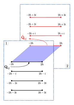
Figure 3: Cut structure of the ${\bf Q}$ functions in the physical Riemann section. On the first (second) sheet, ${\bf Q}$ is analytic in the upper (lower) half plane.

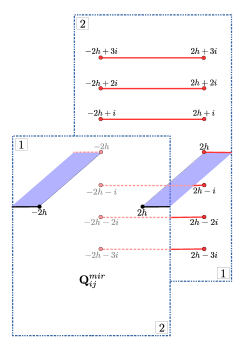
Figure 4: Gluing the two analyticity regions from the sheets $1$ and $2$ of Figure 4, one defines the mirror sheet, with a single long cut.

4.3.1 ${\bf Q}_{ij}$ on the mirror sheet

Let us now prove that, when analytically continued from the upper to the lower half plane passing through the cut $(-2h,2h)$, the matrix ${\bf Q}_{ij}$ is analytic in the whole lower half plane (see Figure 4). Therefore, on an appropriate Riemann section, it has only a pair of long cuts stretching from $\pm 2h$ to infinity (see Figure 4). This is a very strong analogy with the $AdS_{5}/CFT_{4}$ case considered in QSC .

We start by observing that, using (62) and the second equation in (61), the discontinuity relation (60) can be put in the form

$$\widetilde{{\bf Q}}_{ij}={\bf Q}_{mn}\,\left(\delta_{i}^{m}-\tau_{i}\,\tau^{m}\right)\,\left(\delta_{j}^{n}-\tau_{j}\,\tau^{n}\right)\equiv{\bf Q}_{mn}\,f_{i}^{m}\,f_{j}^{n},$$ (63)

where we have defined a $2i$-periodic matrix function $f_{i}^{j}\equiv\delta_{i}^{j}-\tau_{i}\,\tau^{j}$. This relation can be recast as

$$\widetilde{{\bf Q}}_{ij}=\left(Q_{b|m}^{-}\,{\bf P}^{ab}\,Q_{a|n}^{-}\right)\,\,f_{i}^{m}\,f_{j}^{n}={\bf P}^{ab}\,(Q_{b|i}^{\text{LHPA}})^{-}\,(Q_{a|j}^{\text{LHPA}})^{-},$$ (64)

where

$$Q_{a|i}^{\text{LHPA}}\equiv Q_{a|j}\,(f^{j}_{i})^{+}=Q_{a|i}-Q_{a|j}\,(\tau^{j})^{+}\,\tau_{i}^{+}=Q_{a|i}+\nu_{a}^{+}\,(\nu^{b})^{+}\,Q_{b|i}.$$ (65)

We will now show that $Q_{a|i}^{\text{LHPA}}$ has no branch cuts in the lower half plane (hence the superscript LHPA – Lower Half Plane Analytic). Therefore, the representation (64) manifestly shows that the same is true for $\widetilde{{\bf Q}}_{ij}$, implying that ${\bf Q}$ has a single long cut on the mirror Riemann sheet.

To prove that $Q_{a|i}^{\text{LHPA}}$ has no cuts in the lower half plane, we can exploit the fact that, due to the periodicity of $f_{i}^{j}(u)$, it satisfies the same fourth order difference equation (40) fulfilled by $Q_{a|i}$. Therefore, it is sufficient to check that it has no cut on the lines $\text{Im}(u)=-1/2$, $-3/2$: the difference equation (40) will then automatically imply that it is analytic everywhere in the lower half plane. This leaves us with just two conditions to check. The first discontinuity to study is

$$\triangle(\,(Q_{a|i}^{\text{LHPA}})^{-}\,)=\triangle(\,Q_{a|i}^{-}-Q_{a|j}^{-}\,\tau^{j}\,\tau_{i}\,),$$ (66)

where we are using the notation $\triangle(\mathcal{G})=\mathcal{G}-\widetilde{\mathcal{G}}$. From the first relation in (53), we find

$$\triangle(Q_{a|i}^{-}) \equiv Q_{a|i}^{-}-\widetilde{Q}_{a|i}^{-}=-Q_{a|k}^{+}\,\kappa^{kl}\,\left({\bf Q}_{li}-\widetilde{\bf Q}_{li}\right)$$ (67)

$$= -Q_{a|k}^{+}\,\kappa^{kl}\,\left(\tau_{l}\,\widetilde{\tau}_{i}-\tau_{i}\,\widetilde{\tau}_{l}\right),$$ (68)

where we used (61) in the last step. We may now to use the following identities, found by inverting (57),(58):

$$\nu_{a}=-Q_{a|i}^{+}\,\kappa^{ij}\,\widetilde{\tau}_{j},\;\;\;\;\;\;\nu_{a}=-Q_{a|i}^{-}\tau^{i},$$ (69)

to transform (68) into

$$\triangle(Q_{a|i}^{-})=\widetilde{\nu}_{a}\,\widetilde{\tau}_{i}-\nu_{a}\,\tau_{i}=-\triangle(\nu_{a}\,\tau_{i})=\triangle(Q_{a|j}^{-}\,\tau^{j}\,\tau_{i}).$$ (70)

The last equality shows the vanishing of the discontinuity (66). A completely analogous calculation would show that

$$\triangle\left[(Q^{a}_{\,|j})^{-}\,(f^{j}_{i})^{[-2]}\right]=0,$$ (71)

therefore also the next discontinuity is trivial

$$\triangle\left[\,(Q_{a|i}^{\text{LHPA}})^{[-3]}\,\right]={\bf P}_{ab}^{[-2]}\;\triangle\left[(Q^{a}_{\,|j})^{-}\;(f^{j}_{i})^{[-2]}\right]=0,$$ (72)

which concludes the proof.

4.3.2 Vector form of the ${\bf Q}\tau$-system

We may rewrite the discontinuity equations (61) in an alternative form, more similar to the ${\bf P}\mu$-system. To do this, let us rearrange the components of ${\bf Q}_{ij}^{\bf{5}}$ into a five-vector:

$${\bf Q}_{I}(u)\equiv-\frac{1}{2}\,\left({\bf Q}_{ij}^{\bf{5}}(u)\,\bar{\Sigma}^{ij}_{I}\right),\;\;\;(I=1,\dots,5),$$ (73)

or equivalently

$${\bf Q}_{ij}^{\bf{5}}(u)=(\Sigma_{I})_{ij}\,\rho^{IJ}\,{\bf Q}_{J}(u),$$ (74)

where we are using the matrices $\Sigma^{I}$ and the metric $\rho^{IJ}$ defined in Section 2. In components, this definition reads

$${\bf Q}_{I} = -\left({\bf Q}_{12},{\bf Q}_{13},{\bf Q}_{24},{\bf Q}_{34},\frac{1}{2}\,({\bf Q}_{14}+{\bf Q}_{23})\right),$$ (75)

$${\bf Q}_{ij}^{\bf 5} = \left(\begin{array}[]{ccccc}0&-{\bf Q}_{1}&-{\bf Q}_{2}&-{\bf Q}_{5}\\ {\bf Q}_{1}&0&-{\bf Q}_{5}&-{\bf Q}_{3}\\ {\bf Q}_{2}&{\bf Q}_{5}&0&-{\bf Q}_{4}\\ {\bf Q}_{5}&{\bf Q}_{3}&{\bf Q}_{4}&0\end{array}\right).$$ (80)

It is also convenient to define

$$\omega_{IJ}(u) \equiv \tau^{k}(u)\,(\Sigma_{IJ})_{k}^{\,i}\,\tau_{i}(u),\;\;\;\;\;\;\psi_{I}(u)\equiv{\tau}^{m}(u)\,\kappa_{mi}\,\bar{\Sigma}_{I}^{ij}\,\tau_{j}(u),$$ (81)

or explicitly:

$$\omega_{IJ}=\left(\begin{array}[]{ccccc}0&\tau_{1}\tau^{4}&-\tau_{2}\tau^{3}&-\tau^{3}\tau_{3}-\tau^{4}\tau_{4}&\frac{1}{2}(\tau_{2}\tau^{4}-\tau_{1}\tau^{3})\\ -\tau_{1}\tau^{4}&0&-\tau^{3}\tau_{3}-\tau_{1}\tau^{1}&\tau_{3}\tau^{2}&\frac{1}{2}(\tau_{1}\tau^{2}+\tau_{3}\tau^{4})\\ \tau_{2}\tau^{3}&\tau^{3}\tau_{3}+\tau_{1}\tau^{1}&0&-\tau_{4}\tau^{1}&\frac{1}{2}(\tau_{2}\tau^{1}+\tau_{4}\tau^{3})\\ \tau^{3}\tau_{3}+\tau^{4}\tau_{4}&-\tau_{3}\tau^{2}&\tau_{4}\tau^{1}&0&\frac{1}{2}(\tau^{1}\tau_{3}-\tau^{2}\tau_{4})\\ \frac{1}{2}(\tau_{1}\tau^{3}-\tau_{2}\tau^{4})&-\frac{1}{2}(\tau_{1}\tau^{2}+\tau_{3}\tau^{4})&-\frac{1}{2}(\tau_{2}\tau^{1}+\tau_{4}\tau^{3})&\frac{1}{2}(\tau^{2}\tau_{4}-\tau^{1}\tau_{3})&0\end{array}\right),$$ (82)

$$\psi_{I}=\left(-\tau_{1}\tau^{3}-\tau_{2}\tau^{4},\,\tau_{1}\tau^{2}-\tau_{3}\tau^{4},\,-\tau_{2}\tau^{1}+\tau_{4}\tau^{3},\,-\tau^{2}\tau_{4}-\tau^{1}\tau_{3},\,\tau_{2}\tau^{2}+\tau_{3}\tau^{3}\right).$$ (83)

From (56),(59), it is simple to prove that the components of $\omega_{IJ}(u)$ are $i$-periodic functions, while the components of $\psi_{I}$ are anti-periodic under the same shift:

$$\omega_{IJ}^{[+2]}=\omega_{IJ},\;\;\;\;\;\psi_{I}^{[+2]}=-\psi_{I}.$$ (84)

In terms of these new variables, the nonlinear constraints (47),(62) take the form

$$\frac{{\bf Q}_{\circ}^{2}}{16}-1={\bf Q}_{5}^{2}-{\bf Q}_{2}\,{\bf Q}_{3}+{\bf Q}_{1}\,{\bf Q}_{4}\;,\;\;\;\;\;\;\;\;\omega_{IJ}\,\rho^{JK}\,\omega_{KL}=-\frac{1}{2}\,\psi_{I}\,\psi_{L}\;,\;\;\;\;\;\;\;\;\psi_{I}\,\rho^{IJ}\,\psi_{J}=0\;,$$ (85)

while the discontinuity equations (61) can be rewritten as

$$\widetilde{{\bf Q}}_{I}-{\bf Q}_{I} =-\omega_{IJ}\;\rho^{JK}\,{\bf Q}_{K}+\frac{1}{4}\,\psi_{I}\,{\bf Q}_{\circ}, \widetilde{\omega}_{IJ}-\omega_{IJ} ={\bf Q}_{I}\,\widetilde{{\bf Q}}_{J}-{\bf Q}_{J}\,\widetilde{{\bf Q}}_{I},$$

$$\widetilde{{\bf Q}}_{\circ}-{{\bf Q}}_{\circ} =2\,\psi_{J}\,\rho^{JK}\,{\bf Q}_{K}, \widetilde{\psi}_{I}-\psi_{I} =\frac{1}{2}\,\left({\bf Q}_{I}\,\widetilde{{\bf Q}}_{\circ}-{\bf Q}_{\circ}\,\widetilde{{\bf Q}}_{I}\right).$$

4.4 Reduction to $4\leftrightarrow\bar{4}$ symmetric states

In this Section we consider the reduction of the QSC equations to a large subsector characterized by perfect symmetry between the contributions of A- and B-type excitations. In terms of the ABA, this subsector is characterized by the equality of the sets of momentum-carrying Bethe roots, $\left\{u_{4,k}\right\}_{k=1}^{K_{4}}=\left\{u_{\bar{4},k}\right\}_{k=1}^{K_{\bar{4}}}$. As discussed in Appendix A, this case is selected by the conditions:

$${\bf P}_{5}={\bf P}_{6},\quad\nu^{a}=\kappa^{ab}\nu_{b}.$$ (86)

In this case we have the relation ${\bf P}^{ab}=\kappa^{al}\,{\bf P}_{lm}\,\kappa^{mb}$ and we see that necessarily, $e^{i\mathcal{P}}$ is either $1$ or $-1$. By studying the large-$u$ asymptotics of equation (40), we find that, in this case, the elements of the matrices $Q_{a|i}$, $Q^{a|i}$ may be chosen as related by the symmetry:

$$Q^{a}_{\,|i}=-e^{i\mathcal{P}}\,\kappa^{ab}\,Q_{b|j}\,\mathbb{K}^{j}_{i},$$ (87)

with

$$\mathbb{K}^{i}_{j}=\left(\begin{array}[]{cccc}1&0&0&0\\ 0&-1&0&0\\ 0&0&-1&0\\ 0&0&0&1\end{array}\right).$$ (88)

This means also that

$$Q_{a|i}\,\kappa^{ab}\,Q_{b|k}\,\hat{\kappa}^{kl}=\delta_{i}^{\,l},$$ (89)

where $\hat{\kappa}^{ki}\equiv-e^{i\mathcal{P}}\,(\kappa\,\mathbb{K})^{ki}=-e^{i\mathcal{P}}\,(\mathbb{K}\,\kappa)^{ki}$. The symmetry imposes the following condition:

$${\bf Q}_{ij}=-\mathbb{K}_{i}^{k_{1}}\,{\bf Q}_{k_{1}k_{2}}\,\mathbb{K}^{k_{2}}_{j}-\frac{\kappa_{ij}}{2}\,{{\bf Q}}_{\circ},\;\;\;\;\;$$ (90)

which implies

$${\bf Q}^{\bf{5}}_{ij}=-\mathbb{K}_{i}^{k_{1}}\,{\bf Q}^{\bf{5}}_{k_{1}k_{2}}\,\mathbb{K}^{k_{2}}_{j}.$$ (91)

Taking (86),(87) into account in (55), we see that in this subsector the periodicity of $\tau_{i}$ is enhanced to

$$\tau_{i}^{[+2]}=\tau_{k}\,\mathbb{K}^{k}_{i},$$ (92)

which means that $\tau_{1}$ and $\tau_{4}$ are $i$-periodic, while $\tau_{2}$, $\tau_{3}$ are $i$-anti-periodic. Since we expect all these functions to have power-like asymptotics for physical operators, we see, from the condition of anti-periodicity, that

$$\lim_{u\rightarrow\pm\infty}\tau_{2}=\lim_{u\rightarrow\pm\infty}\tau_{3}=0.$$ (93)

This resut will be important in the following. Finally, in terms of the variables of Section 4.3.2, the reduction to the symmetric subsector can be obtained setting ${\bf Q}_{5}=\psi_{5}=\omega_{5I}=\omega_{I5}=0$.

5 Asymptotics and global charges

5.1 Large-$u$ behaviour and quantum numbers

The Riemann-Hilbert type equations described in Sections 3 and 4 have to be supplemented with appropriate constraints on the large-$u$ behaviour of the functions entering the QSC. We will assume, in analogy with Gromov:2014caa , that all the functions we have described scale as powers of $u$ for large values of the spectral parameter, in particular

$${\bf P}_{A}(u)\sim\mathcal{A}_{A}\,u^{-M_{A}}.$$ (94)

An important observation is that, since the ${\bf P}$ functions have a single short cut on the first Riemann sheet, they must have trivial monodromy around infinity, which forces $M_{A}\in\mathbb{Z}$. For the spectrum problem, we found that these parameters should be paired up as $M_{1}=-M_{4}$, $M_{2}=-M_{3}$, $M_{5}=-M_{6}$. The three independent integer parameters contained in the asymptotics (94) can be identified with the three $SO(6)$ R-charges $J_{1},J_{2},J_{3}$, corresponding to three angular momenta parametrizing the motion of the string in $CP^{3}$:

$$M_{A}=\left(J_{2}+1,\,J_{1},\,-J_{1},\,-J_{2}-1,\,-J_{3},\,J_{3}\right).$$ (95)

The $AdS_{4}$ charges $\Delta$ and $S$, corresponding to the conformal dimension and spin of the gauge theory operator, respectively, enter the QSC through the asymptotics of the $\nu_{a}$ functions. Equivalently, they can be read off the coefficients $\mathcal{A}_{A}$ in (94), which satisfy the constraints

$$\mathcal{A}_{B}\,\mathcal{A}^{B}=2\,\frac{\prod_{I=1}^{5}\left(M_{B}-\hat{M}_{I}\right)}{\prod_{C\neq B}^{6}(M_{B}-M_{C})},\;\;\;\;(B=1,\dots,6),$$ (96)

(with no summation implied on the index $B$), where the 5-vector $\hat{M}$ is defined as

$$\hat{M}_{I}=\left(\Delta+S+1\,,\,\Delta-S\,,\,-\Delta+S\,,\,-\Delta-S-1\,,\,0\right).$$ (97)

The above identifications (95),(97) between parameters and quantum numbers will be deduced in Appendix D considering the weak coupling limit of the QSC equations. Notice that the charges $(\Delta,S,J_{1},J_{2},J_{3})$ used above are defined relatively to the Dynkin diagram of Figure 6. We remind the reader that, for supersymmetric algebras, the definition of the charges depends on a choice of grading of the Dynkin diagram; if a different grading were chosen, relations (95) and (97) would be slightly different. However, we stress that the parameters $M_{A}$ and $\hat{M}_{I}$ appearing in the asymptotics of the QSC are invariant under these changes, and unambiguously associated to a given multiplet (see Gromov:2014caa for a detailed discussion). Concretely, we may read the charges from the Asymptotic Bethe Ansatz description of the state:

$$J_{1}=L-K_{1},\quad J_{2}=L-K_{4}-K_{\bar{4}}+K_{3},\quad J_{3}=K_{4}-K_{\bar{4}},$$ (98)

$$\Delta-S=L+K_{2}-K_{1}+\gamma,\quad\Delta+S=L+K_{3}-K_{2}+\gamma,$$ (99)

where $L$ is the length parameter and $K_{i}$ denotes the number of Bethe roots of type $i$ in the so-called $\eta=+1$ version of the ABA Gromov:2008qe , while $\gamma$ is the anomalous dimension. For more details and a dictionary between different forms of the ABA, see Appendix E.

The large-$u$ asymptotics of the matrix $Q_{a|i}(u)$ may be determined by studying (40). There are four possible asymptotic behaviours where $Q_{a|i}$ scales as a power of $u$, parametrized in terms of the charges $M_{A}$, $\hat{M}_{I}$ entering the equation through (94),(96). By choosing a suitable linear combination of solutions, we shall impose that different columns of $Q_{a|i}$ have distinct leading asymptotics, ordered in such a way that $|Q_{a|i}|>|Q_{a|j}|$ for $i<j$ for large $u$. To describe the possible scaling behaviours, it is convenient to introduce:

$$\mathcal{N}_{a} = \left(\frac{1}{2}(-M_{1}-M_{2}-M_{5}),\frac{1}{2}(-M_{1}+M_{2}+M_{5}),\frac{1}{2}(M_{1}-M_{2}+M_{5}),\frac{1}{2}(M_{1}+M_{2}-M_{5})\right),$$

$$\mathcal{N}^{a} = \left(\frac{1}{2}(M_{1}+M_{2}+M_{5}),\frac{1}{2}(M_{1}-M_{2}-M_{5}),\frac{1}{2}(-M_{1}+M_{2}-M_{5}),\frac{1}{2}(-M_{1}-M_{2}+M_{5})\right),$$

$$\hat{\mathcal{N}}_{i} = \left(\frac{1}{2}(\hat{M}_{1}+\hat{M}_{2}),\frac{1}{2}(\hat{M}_{1}-\hat{M}_{2}),\frac{1}{2}(\hat{M}_{2}-\hat{M}_{1}),\frac{1}{2}(-\hat{M}_{1}-\hat{M}_{2})\right).$$ (100)

With these definitions, we have

$${\bf P}_{ab}(u)\sim u^{\mathcal{N}_{a}+\mathcal{N}_{b}},\;\;\;\;\;Q_{a|i}(u)\sim u^{\mathcal{N}_{a}+\hat{\mathcal{N}}_{i}},\;\;\;\;\;\;Q^{a}_{\,|i}(u)\sim u^{\mathcal{N}^{a}+\hat{\mathcal{N}}_{i}},$$ (101)

while $\nu_{a}$ and $\nu^{a}$ have the same leading asymptotic behaviour as $Q_{a|1}$, $Q^{a}_{\,|1}$, namely:

$$\nu_{a}(u)\sim u^{\mathcal{N}_{a}+\hat{\mathcal{N}}_{1}},\quad\nu^{a}(u)\sim u^{\mathcal{N}^{a}+\hat{\mathcal{N}}_{1}}.$$ (102)

The asymptotics of ${\bf Q}_{ij}$ can be computed from the definition (46), and turn out to be, for the vector components,

$${\bf Q}_{I}(u) \simeq \left(\mathcal{B}_{1}\,u^{\hat{M}_{1}-1},\mathcal{B}_{2}\,u^{\hat{M}_{2}-1},\mathcal{B}_{3}\,u^{-\hat{M}_{2}-1},\mathcal{B}_{4}\,u^{-\hat{M}_{1}-1},\frac{\mathcal{B}_{5}}{u}\right),$$ (103)

where the coefficients $\mathcal{B}_{I}$ are constrained by consistency conditions similar to (96):

$$\mathcal{B}_{I}\,\mathcal{B}^{I} = \frac{1}{2}\,\frac{\prod_{A=1}^{6}\left(\hat{M}_{I}-M_{A}\right)}{\prod_{J\neq I}^{5}(\hat{M}_{I}-\hat{M}_{J})},\;\;\;\;(I=1,\dots,5),$$ (104)

$$\mathcal{B}_{5} = \frac{i}{2}\frac{M_{1}\,M_{2}\,M_{5}}{\hat{M}_{1}\,\hat{M}_{2}},$$ (105)

(with no summation on the index $I$ in (104)). The trace part satisfies

$${\bf Q}_{\circ}(u)=4+\frac{2\,\mathcal{C}}{u^{2}}+\mathcal{O}\left(\frac{1}{u^{3}}\right),$$ (106)

where the constant $\mathcal{C}$ coincides with the value of the $OSp(4|6)$ Casimir:

$$\mathcal{C}=\frac{1}{4}\left(\hat{M}_{1}^{2}+\hat{M}_{2}^{2}-M_{1}^{2}-M_{2}^{2}-M_{5}^{2}\right).$$ (107)

A derivation of the constraints (96),(104-107) is discussed in Appendix C. Finally, let us comment on the asymptotics of the four functions $\tau_{i}(u)$. Since the latter are $2i$-periodic, and by construction grow less than exponentially for large $u$, they must approach a vector of constants at infinity. There is a certain amount of freedom in normalizing these constants, but we expect that for any physical state the components of $\tau_{i}$ with $i=2,3$ always vanish at large $u$:

$$\lim_{u\rightarrow\pm\infty}\tau_{2}(u)=\lim_{u\rightarrow\pm\infty}\tau_{3}(u)=0.$$ (108)

In Section 4.4 we established (108) for the class of $4\leftrightarrow{\bar{4}}$-symmetric operators. While we do not have a fully rigorous argument, we postulate that (108) is true in general even for nonsymmetric states. As we discuss in Section 6, the asymptotics (108) implies the quantization of the spin and is the main ingredient for deriving the so-called gluing conditions, a powerful set of constraints encoding the main analytic properties of the system.

5.2 Classical limit

The algebraic curve describing IIA string solutions on $AdS_{4}\times CP^{3}$ in the classical limit where $\Delta,S,J_{i}=\mathcal{O}(h)$, $h\sim\sqrt{\lambda/2}\rightarrow\infty$ was proposed in Gromov:2008bz . In particular, a monodromy matrix was built on the basis of the Lax connection found in Stefanski:2008ik ; Arutyunov:2008if and its eigenvalues $\lambda_{a}\equiv e^{iq_{a}}$ were shown to define a ten-sheeted Riemann surface covering the domain of the relevant strong coupling spectral parameter, the Zhukovsky variable $x$. It is convenient to consider the logarithm of the eigenvalues, the so-called quasi-momenta, naturally grouped as $\{q_{3},q_{4},q_{5},-q_{3},-q_{4},-q_{5}\}$ and $\{q_{1},q_{2},-q_{1},-q_{2}\}$, corresponding respectively to the $SO(6)$ invariant $CP^{3}$ and the $Sp(4)$ invariant $AdS_{4}$ sectors of the monodromy matrix. The quasi-momenta are connected by logarithmic cuts, which may be viewed as condensates of Bethe roots. Classical string solutions can be studied by listing algebraic curves satisfying appropriate analytic properties (see Gromov:2008bz for full details), and in particular the charges can be read off the asymptotics of the curve at large values of the spectral parameter:

$$\left(\begin{array}[]{c}q_{1}(x)\\ q_{2}(x)\\ q_{3}(x)\\ q_{4}(x)\\ q_{5}(x)\end{array}\right)\sim\frac{1}{h\,x}\left(\begin{array}[]{c}\Delta+S\\ \Delta-S\\ J_{1}\\ J_{2}\\ J_{3}\end{array}\right),\;\;\;x\sim\infty,$$ (109)

where the quasi-momenta are ordered as in Gromov:2008bz . In the classical limit, we expect that some of the ${\bf P}$ and ${\bf Q}$ functions of the QSC are related to the quasi-momenta as follows:

$${\bf P}_{1}(u)\sim e^{-h\int^{u/h}{\bf q}_{4}(z)dz},\;\;\;\;{\bf P}_{4}(u)\sim e^{+h\int^{u/h}{\bf q}_{4}(z)dz},$$ (110)

$${\bf P}_{2}(u)\sim e^{-h\int^{u/h}{\bf q}_{3}(z)dz},\;\;\;\;{\bf P}_{3}(u)\sim e^{+h\int^{u/h}{\bf q}_{3}(z)dz},$$ (111)

$${\bf P}_{5}(u)\sim e^{+h\int^{u/h}{\bf q}_{5}(z)dz},\;\;\;\;{\bf P}_{6}(u)\sim e^{-h\int^{u/h}{\bf q}_{5}(z)dz},$$ (112)

$${\bf Q}_{1}(u)\sim e^{+h\int^{u/h}{\bf q}_{1}(z)dz},\;\;\;\;{\bf Q}_{4}(u)\sim e^{-h\int^{u/h}{\bf q}_{1}(z)dz},$$ (113)

$${\bf Q}_{2}(u)\sim e^{+h\int^{u/h}{\bf q}_{2}(z)dz},\;\;\;\;{\bf Q}_{3}(u)\sim e^{-h\int^{u/h}{\bf q}_{2}(z)dz},$$ (114)

where we use the notation ${\bf q}_{i}(z)\equiv q_{i}(z/2+\sqrt{z-2}\sqrt{z+2}/2)$ for the quasi-momenta parametrized in terms of the rescaled spectral parameter $z=u/h$, which is the natural variable at strong coupling. Using (109), one can verify that (110)-(114 are nicely consistent with our asymptotics (95)-(97).

Some of the limits (114), particularly the ones for ${\bf P}_{1}$, ${\bf P}_{2}$, ${\bf Q}_{1}$, ${\bf Q}_{2}$, ${\bf P}_{5}$, ${\bf P}_{6}$, can be derived from the large volume solution of the QSC, see the Section 7.3 below. In the rest of this Section, we discuss other consistency checks of the semi-classical identifications, as this will illustrate interesting analogies between classical and quantum curve (for a similar treatment, see Section 6 in Gromov:2014caa ).

One of the important features of the classical curve is the inversion symmetry Gromov:2008bz :

$$\left(\begin{array}[]{c}q_{1}(1/x)\\ q_{2}(1/x)\\ q_{3}(1/x)\\ q_{4}(1/x)\\ q_{5}(1/x)\end{array}\right)=\left(\begin{array}[]{c}-q_{2}(x)\\ -q_{1}(x)\\ 2\pi m-q_{4}(x)\\ 2\pi m-q_{3}(x)\\ q_{5}(x)\end{array}\right),\quad m\in\mathbb{Z}$$ (115)

which is inherited by the transformation property of the monodromy matrix under the $\mathbb{Z}_{4}$ automorphism of $OSp(4|6)$ Stefanski:2008ik ; Arutyunov:2008if . Let us discuss how this property is related to the Riemann-Hilbert type equations (32),(61) valid for ${\bf P}$ and ${\bf Q}$ at finite coupling.

Consider first the case of ${\bf P}$ functions. Their values on the second sheet is parametrized in terms of the matrix $\mu_{AB}$ which is $i$-periodic on the mirror section. In terms of the natural variable $z=u/h$, this periodicity becomes $i/h\rightarrow 0$ at strong coupling. Therefore, assuming that $\mu_{AB}$ admits a smooth classical limit, it must freeze to a constant value independent of $z$ Gromov:2014caa , which can be normalized to be of order $\mathcal{O}(1)$. From two of the QSC equations (16), we then find

$$\widetilde{\bf P}_{1}\sim{\bf P}_{3},\quad\widetilde{\bf P}_{2}\sim{\bf P}_{4},$$ (116)

where we have dropped all terms containing ${\bf P}_{1}$ and ${\bf P}_{2}$ on the rhs, since we see from (110),(111) that they are exponentially suppressed as $h\rightarrow\infty$. On the other hand, analytically continuing to the second sheet the semi-classical expressions for ${\bf P}_{1}$ and ${\bf P}_{2}$, and using the inversion symmetry (115), one finds (see Gromov:2014caa for details)

$$\widetilde{\bf P}_{1}\sim e^{+h\int^{u/h}{\bf q}_{3}(z)dz},\quad\widetilde{\bf P}_{2}\sim e^{+h\int^{u/h}{\bf q}_{4}(z)dz}.$$ (117)

The comparison between (117) and (116) motivates the semi-classical identification for ${\bf P}_{3}$ and ${\bf P}_{4}$.

This analysis cannot be straightforwardly repeated for the ${\bf Q}$ functions, since the functions $\tau_{i}$ are periodic only on the short-cuts section, which becomes analytically disconnected from the $z$-plane at strong coupling. However, the inversion symmetry has a quantum analogue in the gluing conditions discussed in Section 6, which connect $\widetilde{\bf Q}_{ij}$ and the complex conjugate functions $\overline{\bf Q}_{ij}$. From the analytic continuation of (110)-(114), combined with the inversion symmetry, we may infer that in the classical limit

$${\widetilde{\bf Q}}_{3}\propto\overline{{\bf Q}}_{1},\quad{\widetilde{\bf Q}}_{4}\propto\overline{{\bf Q}}_{2}.$$ (118)

This is indeed consistent with the results of Section 6.

As a last comment, notice that there is no classical analogue for two of the components of the matrix ${\bf Q}_{ij}$, namely the functions ${\bf Q}_{5}$ and ${\bf Q}_{\circ}$, which enter the basic Riemann-Hilbert constraints at finite coupling, but appear to completely decouple from the dynamics in the classical limit. This is a peculiar feature, as compared with the case of $AdS_{5}/CFT_{4}$, and it would be important to find a proper interpretation. One may also speculate that there is a connection with the fact that part of the classical string solutions in ABJM theory are not captured by the classical spectral curve Sorokin:2011mj .

5.3 Unitarity conditions

The structure of the QSC also appears to automatically implement the unitarity bounds satisfied by the charges of a physical state. The discussion here will be very similar to the argument of Section C.2 of Gromov:2014caa , so we will only sketch the main points. From the perspective of the QSC, the unitarity bounds arise from the requirement that the powers appearing in the asymptotics of ${\bf P}$ and ${\bf Q}$ functions are all distinct. This condition is very natural, since otherwise expressions like (96) and (104) for the coefficients $\mathcal{A}_{A}$, $\mathcal{B}_{I}$ would become singular. A further condition appears to be needed, namely that, for all consistent solutions of the QSC, the powers entering the asymptotics of ${\bf Q}$ functions are greater than the ones entering the asymptotics of ${\bf P}$ functions: precisely, $|M_{A}|<|\hat{M}_{I}|$, $I\neq 5$. While it is more difficult to motivate this bound from first principles, it can be verified that it holds at weak coupling or in the large volume limit. Assuming a (purely conventional) ordering of magnitude for the components of ${\bf P}_{A}$ and ${\bf Q}_{I}$, we can therefore argue that all non-singular solutions of the QSC can be found restricting our attention to

$$\hat{M}_{1}>\hat{M}_{2}>M_{2}>M_{1}>|M_{5}|.$$ (119)

With the identification (95),(97), we find that these conditions coincide with the unitarity bounds

$$J_{2}\geq|J_{3}|,\;\;\;J_{1}\geq 2+J_{2},\;\;\;S\geq 0,\;\;\;\Delta>S+J_{1},$$ (120)

or equivalently, in terms of excitation numbers (see Minahan:2009te ):

$$L+K_{3}-2K_{4}\geq 0,\;\;L+K_{3}-2K_{\bar{4}}\geq 0,\;\;\;K_{4}+K_{\bar{4}}-K_{3}\geq 2+K_{1},$$ (121)

$$K_{3}+K_{1}\geq 2\,K_{2},\;\;\;\;K_{2}+\gamma>0.$$ (122)

As a final comment, notice that, in principle, some of the inequalities (119) could be saturated exactly in the weak coupling limit, where $\gamma\rightarrow 0$. Since the parameters $M_{A}$, as well as $\hat{M}_{2}-\hat{M}_{1}$ (see Section 6) are quantized, this is possible only for the condition $\hat{M}_{2}>M_{2}$. The saturation of this bound for $\gamma\rightarrow 0$ is equivalent to the multiplet shortening condition:

$$\Delta^{(0)}-S-J_{1}=0,$$ (123)

where $\Delta^{(0)}$ is the classical conformal dimension, or equivalently $K_{2}=0$ in terms of excitation numbers. The states satisfying (123) have a peculiar characteristic in the QSC, namely they are the ones for which one of the ${\bf P}$ functions vanishes at weak coupling. This is shown by the fact that for these operators $\mathcal{A}_{2}\,\mathcal{A}_{3}\rightarrow 0$ as $\hat{M}_{2}-M_{2}\rightarrow 0$ in (96).

6 Gluing conditions and spin quantization

We shall now derive an exact relation (valid for real values of the charges) connecting the values of ${\bf Q}_{ij}$ on the second sheet to the values of the complex conjugate function $\overline{{\bf Q}}_{ij}$. A similar result was first found in the $AdS_{5}/CFT_{4}$ context and exploited to solve the QSC in various regimes Gromov:2015wca ; Gromov:2015vua . In particular the equations presented below may be used to solve the QSC numerically at finite coupling ContiNumerical . For the derivation, we need an important technical assumption: we require that the matrix elements $Q_{a|i}$ can be expanded at large-$u$ as

$$Q_{a|i}(u)\sim u^{\mathcal{N}_{a}+\hat{\mathcal{N}}_{i}}\,\sum_{m=0}^{\infty}\frac{B_{(a|i),m}}{u^{m}},\;\;\;\;u\rightarrow+\infty.$$ (124)

In words, (124) means that there is no mixing among the powers occurring in the asymptotics of different columns of $Q_{a|i}$. This condition was dubbed “pure asymptotics” in Gromov:2015vua , and can always be enforced using the freedom to take linear combinations of the columns of $Q_{a|i}$. We also assume that, for real values of the charges and the coupling, ${\bf P}_{ab}$ can be chosen to be real. Under these conditions, the conjugate matrix elements $\overline{Q}_{a|i}$ satisfy the same difference equation (40) as $Q_{a|i}$. This implies that the two matrices are related through

$$\overline{Q}_{a|i}(u)=Q_{a|j}(u)\;(\Omega^{j}_{i}(u))^{+},$$ (125)

where $\Omega^{j}_{i}(u)$ is a $2i$-periodic function of $u$: $\Omega^{i}_{j}(u+2i)=\Omega^{i}_{j}(u)$. The condition of pure asymptotics (124) implies that, as $u\rightarrow\infty$, the matrix $\Omega^{i}_{j}$ becomes diagonal. Now, we recall the discontinuity relation (63):

$${\widetilde{\bf Q}}_{ij}(u)=f_{i}^{l}(u)\,{{\bf Q}}_{lk}(u)\,f^{k}_{j}(u),$$ (126)

where $f_{i}^{j}(u)=\delta_{i}^{j}-\tau_{i}(u)\,\tau^{j}(u)$, which, combined with (125), gives

$$\widetilde{{\bf Q}}_{ij}=\mathcal{L}_{i}^{l}\;\kappa_{lk}\;\overline{{\bf Q}}^{km}\;\kappa_{mn}\;\mathcal{L}^{n}_{j},$$ (127)

with

$$\mathcal{L}^{i}_{l}(u)=(f(u)\,{\Omega}^{-1}(u))_{i}^{j}.$$ (128)

The crucial observation is now that $\mathcal{L}^{i}_{j}(u)$ must be a constant independent of $u$. In fact, the definition (128) can be rewritten as

$$\mathcal{L}^{j}_{i}=f_{i}^{k}\,Q_{a|k}^{-}\,(\overline{Q}^{a|j})^{-}=(Q_{a|i}^{\text{LHPA}})^{-}\,(\overline{Q}^{a|j})^{-},$$

and the last equality shows manifestly that $\mathcal{L}^{j}_{i}$ has no cuts in the upper half plane, since this property is true for both $Q_{a|i}^{\text{LHPA}}$ and $\overline{Q}^{a|j}$. Because of its $2i$-periodicity, $\mathcal{L}^{i}_{j}$ is then entire in $u$, and, since it does not grow exponentially, it must be a constant.

To determine the form of $\mathcal{L}_{i}^{j}$, we can study its definition at large $u$, where $\Omega^{i}_{j}$ becomes diagonal and many of the matrix elements of $f^{i}_{j}$ vanish due to the fact that $\tau_{2},\,\tau_{3}\rightarrow 0$. The structure is further specified by several consistency conditions. For instance, since $\mathcal{L}$ does not depend on $u$, we should certainly impose the equality of the following limits:

$$\mathcal{L}_{i}^{j}=\lim_{u\rightarrow+\infty}\left(f(u)\,\Omega^{-1}(u)\right)_{i}^{j}=\lim_{u\rightarrow-\infty}\left(f(u)\,\Omega^{-1}(u)\right)_{i}^{j}.$$ (129)

To exploit this constraint, notice that the constant limits of $\Omega$ at $\pm\infty$ are related as follows:

$$\lim_{u\rightarrow-\infty}\Omega^{i}_{i}(u)=\left(\lim_{u\rightarrow+\infty}\Omega^{i}_{i}(u)\right)\;e^{-2\pi i(\mathcal{N}_{a}+\hat{\mathcal{N}}_{i})}.$$ (130)

This condition can be obtained studying the definition (125) as $u\rightarrow\pm\infty$, using the fact that the asymptotic behaviour of $Q_{a|i}(u)$ ($\overline{Q}_{a|i}(u)$, respectively) as $u\rightarrow-\infty$ must be connected to the one for $u\rightarrow+\infty$ through analytic continuation along a large semicircle in the upper (lower) half plane, where this function is free of singularities. Considering relation (129) for $j=2,3$, and using (130), we find

$$e^{2\pi i(\mathcal{N}_{a}+\hat{\mathcal{N}}_{i})}=1,$$ (131)

for $i=2,3$, $\forall a$. This equation implies that $\hat{M}_{2}-\hat{M}_{1}=2S+1\in\mathbb{Z}$, namely the spin is integer or half-integer. The other conditions in (129) constrain the asymptotics of the non-zero components of $\tau$. Denoting $t_{i,\pm}\equiv\lim_{u\rightarrow\pm\infty}\tau_{i}$, we have in particular

$$t_{1,\pm}\,t_{4,\pm}=\pm i\,e^{i\mathcal{P}}\,\tan(\pi\,\hat{M}_{1}).$$ (132)

Finally, evaluating $\mathcal{L}$ at large $u$ and using (132), relation (127) leads to the gluing conditions:

$$\widetilde{{\bf Q}}_{1} =-\frac{e^{i\pi\hat{M}_{1}}}{y_{1}\,y_{2}\,\cos(\pi\hat{M}_{1})}\,\overline{{\bf Q}}_{1}+\delta_{1}\,\overline{{\bf Q}}_{3},\quad \widetilde{{\bf Q}}_{3} =-\frac{e^{-i\pi\hat{M}_{1}}}{y_{2}\,y_{4}\,\cos(\pi\hat{M}_{1})}\,\overline{{\bf Q}}_{3}+\frac{y_{3}}{y_{2}}\,\delta_{2}\,\overline{{\bf Q}}_{1},$$ (133)

$$\widetilde{{\bf Q}}_{2} =-\frac{e^{i\pi\hat{M}_{1}}}{y_{1}\,y_{3}\,\cos(\pi\hat{M}_{1})}\,\overline{{\bf Q}}_{2}+\frac{y_{2}}{y_{3}}\,\delta_{1}\,\overline{{\bf Q}}_{4},\quad \widetilde{{\bf Q}}_{4} =-\frac{e^{-i\pi\hat{M}_{1}}}{y_{4}\,y_{3}\,\cos(\pi\hat{M}_{1})}\,\overline{{\bf Q}}_{4}+\delta_{2}\,\overline{{\bf Q}}_{2},$$ (134)

$$\widetilde{{\bf Q}}_{\circ} =\overline{{\bf Q}}_{\circ},\quad \widetilde{{\bf Q}}_{5} =-\overline{{\bf Q}}_{5},$$ (135)

where we are using the vector notation defined in Section 4.3.2, $\delta_{1}=e^{-i\mathcal{P}}t_{1,+}^{2}/(y_{1}y_{2})$, $\delta_{2}=-e^{-i\mathcal{P}}t_{4,+}^{2}/(y_{3}y_{4})$, and $y_{i}\equiv\lim_{u\rightarrow+\infty}\Omega^{i}_{i}(u)$. For completeness we point out that the constants $y_{i}$, $\delta_{i}$ may in general depend on the coupling and on various normalization choices. For the implementation of the numerical method, it is only needed to know explicitly the value of $y_{i}$. These constants, which satisfy the consistency conditions $y_{1}=1/y_{4}=1/(y_{1}^{*})$, $y_{2}=1/y_{3}=1/(y_{2}^{*})$, are simply related to the choice of normalization of the $Q_{a|i}(u)$ functions, and can be determined as:

$$y_{i}=(B_{(a|i),0})^{*}/B_{(a|i),0},\quad\forall a.$$ (136)

The relations (133)-(135) are similar to the ones obtained in Gromov:2015wca ; Gromov:2015vua , but slightly more complicated. Indeed, in the $AdS_{5}/CFT_{4}$ context a single $\overline{{\bf Q}}$ function appears on the rhs of the gluing conditions, which are an almost direct lift of the inversion symmetry connecting pairs of quasi-momenta in the classical limit. In the present case, the quantum version is a bit more intricate. In particular, the explicit parametric dependence of the gluing conditions on the charge $\hat{M}_{1}$ needs to be taken into account in order to develop a numerical algorithm ContiNumerical . As a last comment, we observe that the quantization of the spin is a direct consequence of the choice of vanishing asymptotics for two of the components of $\tau$. As shown in Gromov:2015wca , it should be possible to relax this condition and consider continuous values of $S$ by admitting exponentially growing asymptotics in $\tau_{2}$ and $\tau_{3}$.

7 The Q-system

In this Section we show how to embed the previous results into a larger set of functional equations reflecting the $OSp(4|6)$ symmetry. It is important to mention that, while the form of Q-systems associated to $GL(M|N)$-type superalgebras is known (see e.g. Kazakov:2007fy ; Wronskian ; Thook ), there appears to be no comprehensive understanding of this mathematical structure for orthosymplectic superalgebras. Here we take a bottom-up approach to the problem and try to construct the Q-system starting from the Q functions already introduced: ${\bf P}_{A}$, ${\bf Q}_{I}$, $Q_{a|i}$, $Q^{a}_{\,|i}$, together with the relations linking them, equations (42),(43),(46). We will explicitly define new Q functions and prove the validity of a set of functional relations which is rich enough to contain various forms of exact Bethe Ansatz equations (equivalent to the absence of poles for the Q functions) related to the $OSp(4|6)$ symmetry.

Before starting the construction, let us describe some of its main characteristics. Various types of Q functions will be assigned to particular nodes of the Dynkin diagram. We will almost exclusively consider the two versions of the diagram shown in Figures 6, 6, which are the ones associated to the two known forms of Asymptotic Bethe Ansatz. The Q functions will have the general index structure $Q_{\bullet|\ast}$, where $\bullet$ and $\ast$ are (vector or spinor) multi-indices carrying representations of $SO(3,3)$ and $SO(3,2)$, respectively, see Section 2 for notations. Various arguments, and in particular the weak coupling analysis, suggest that Q functions of types ${\bf P}_{A}$ and ${\bf Q}_{I}$ carry Bethe roots associated to the first node of the two diagrams, while the Q functions $Q_{a|i}$, $Q^{a}_{\,|i}$ should be linked to the nodes corresponding to the spinorial representations, see Figures 6, 6. The main task of this Section is to complete the picture by constructing Q functions and functional relations associated to the remaining nodes. In analogy with the Q-system of Gromov:2014caa , and in contrast to the case of standard Lie algebras, for every node of the diagram one may define equations of two basic types – fermionic or bosonic. This feature of supersymmetric Q-systems is known to be related to the existence of different gradings of the Dynkin diagram. Choosing different chains of Q functions, we will recover different sets of exact Bethe equations. Finally, as a non-trivial check of the construction, we will recover the two forms of the ABA equations in the large volume limit.

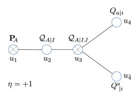
Figure 5: Chain of Q functions corresponding to the $\eta=+1$ grading of the Bethe Ansatz.

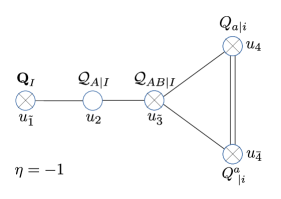
Figure 6: Chain of Q functions corresponding to the $\eta=-1$ grading of the Bethe Ansatz.

7.1 Construction of the Q-system

First step: identifying ${\mathcal{Q}}_{A|I}$

We start the construction by some guesswork. From the form of the Bethe Ansatz, and taking inspiration from Gromov:2014caa , it is natural to expect that one of the functional relations should read:

$$F_{1}: \quad{\mathcal{Q}}_{A|I}^{+}-{\mathcal{Q}}_{A|I}^{-} ={\bf P}_{A}\,{{\bf Q}}_{I}.$$ (137)

We have marked this equation with the symbol $F_{1}$ to point out that it is a fermionic-type Q-system relation, based at the first node of the Dynkin diagram. This equation might be taken as a non-local definition of the $6\times 5$ matrix ${\mathcal{Q}}_{A|I}$. However, this new type of Q functions can also be expressed as an explicit, local combination of the building blocks $Q_{a|i}$, $Q^{a}_{\,|i}$, through the following quadratic combinations:

$$Q_{ab|ij}=Q_{a|i}\,Q_{b|j}-Q_{a|j}\,Q_{b|i}=\text{det}\left(\begin{array}[]{cc}Q_{a|i}&Q_{a|j}\\ Q_{b|i}&Q_{b|j}\end{array}\right),$$ (138)

namely, the $2\times 2$ minors of the $4\times 4$ matrix $\left\{Q_{a|i}\right\}$. Notice that $Q_{ab|ij}$ is antisymmetric in both $(ab)$ and $(ij)$, and therefore has $6\times 6$ independent components. To match the $6\times 5$ components of ${\mathcal{Q}}_{A|I}$ we need of course to project the $(ij)$ indices on the vector representation. The correct identification, which will be important for the derivation of the rest of the Q-system, is simply:

$${\mathcal{Q}}_{A|I}\equiv-\frac{1}{4}\,Q_{ab|ij}\,\bar{\sigma}_{A}^{ab}\,\bar{\Sigma}_{I}^{ij}.$$ (139)

We will show below that this definition implies the validity of (137).

One could also consider the complementary projection on the singlet representation for the $(ij)$ indices, and define:

$${\mathcal{Q}}_{A|\circ}=-\frac{1}{4}Q_{ab|ij}\,\kappa^{ij}\,\bar{\sigma}_{A}^{ab}.$$ (140)

However, it turns out that all Q functions carrying the singlet representation of $SO(3,2)$, such as ${\mathcal{Q}}_{A|\circ}$ and ${\bf Q}_{\circ}$, drop out of the functional relations needed for the derivation of exact Bethe equations. It would be interesting to understand from the algebraic point of view whether they should be considered as part of the Q-system.

7.1.1 Q-system relations for the nodes $1,2,3$

To prove the validity of (137), we start by rewriting the constraint $\text{Pf}({\bf P}_{ab})=1$ as:

$${\bf P}_{ab}\,{\bf P}_{cd}-{\bf P}_{cb}\,{\bf P}_{ad}-{\bf P}_{ac}\,{\bf P}_{bd}=\epsilon_{abcd},$$ (141)

where $\epsilon_{abcd}$ denotes the completely antisymmetric Levi-Civita tensor. Using this identity, it is immediate to prove that

$$Q_{a|\,\left[i\right.}^{+}\,Q_{b|\;\left.j\right]}^{+} = {\bf P}_{aa_{1}}\,{\bf P}_{bb_{1}}\left(Q^{a_{1}}_{\,|\,\left[i\right.}\,Q^{b_{1}}_{\,|j\left.\right]}\right)^{-}$$

$$= \frac{1}{2}\;\epsilon_{aa_{1}bb_{1}}\,\left(Q^{a_{1}}_{\,|\,\left[\right.i}\,Q^{b_{1}}_{\,|j\left.\right]}\right)^{-}+\frac{1}{2}\,{\bf P}_{ab}\;\left({\bf P}_{a_{1}b_{1}}(Q^{a_{1}}_{\,|\left[\right.i})^{-}\,(Q^{b_{1}}_{\,|j\left.\right]})^{-}\right),$$

and, inserting (52), we obtain

$$Q_{ab|ij}^{+}+\frac{1}{2}\,\epsilon_{abcd}\,(Q^{cd}_{\,|ij})^{-}=-{\bf P}_{ab}\,\left({\bf Q}_{ij}+\frac{\kappa_{ij}}{2}{\bf Q}_{\circ}\right).$$ (143)

Projecting on vector indices as in (139) and taking into account simple algebraic identities (see (324)), (143) yields precisely the fermionic equation (137):

$$F_{1}: \quad{\mathcal{Q}}_{A|I}^{+}-{\mathcal{Q}}_{A|I}^{-} ={\bf P}_{A}\,{{\bf Q}}_{I}.$$ (144)

For completeness, we report also the identity obtained by tracing over $(ij)$:

$${\mathcal{Q}}_{A|\circ}^{+}+{\mathcal{Q}}_{A|\circ}^{-}=\frac{1}{2}\,{\bf P}_{A}\,{{\bf Q}}_{\circ}.$$ (145)

As anticipated, (145) is apparently decoupled from the rest of the Q-system and will not play a role in the following considerations. Bosonic-type Q-system relations for the first node can be introduced straightforwardly. They take the standard form:

$$B_{1}: {\bf P}_{A}^{+}\,{\bf P}_{B}^{-}-{\bf P}_{A}^{-}\,{\bf P}_{B}^{+} ={\mathcal{Q}}_{AB|\emptyset},$$ (146)

$$B_{1\ast}: {\bf Q}_{I}^{+}\,{\bf Q}_{J}^{-}-{\bf Q}_{I}^{-}\,{\bf Q}_{J}^{-} ={\mathcal{Q}}_{\emptyset|IJ},$$ (147)

which can be interpreted as definitions of the new two-index objects $Q_{AB|\emptyset}$ and $Q_{\emptyset|IJ}$. These Q functions do not sit on the diagrams in Figures 6, 6, but appear in other choices of gradings, such as the distinguished one (see discussion below).

The construction of functional relations for the second and third nodes is standard and follows the usual fusion rules, cf Gromov:2014caa . In particular, associated to the third node we define the Q functions

$${\mathcal{Q}}_{A|IJ} \equiv {\bf Q}_{I}\,{\mathcal{Q}}_{A|J}^{-}-{\bf Q}_{J}\,{\mathcal{Q}}_{A|I}^{-}={\bf Q}_{I}\,{\mathcal{Q}}_{A|J}^{+}-{\bf Q}_{J}\,{\mathcal{Q}}_{A|I}^{+},$$ (148)

$${\mathcal{Q}}_{AB|I} \equiv {\bf P}_{A}\,{\mathcal{Q}}_{B|I}^{-}-{\bf P}_{B}\,{\mathcal{Q}}_{A|I}^{-}={\bf P}_{A}\,{\mathcal{Q}}_{B|I}^{+}-{\bf P}_{B}\,{\mathcal{Q}}_{A|I}^{+},$$ (149)

which satisfy bosonic-type relations for the second node:

$$B_{2}: {\mathcal{Q}}_{A|IJ}\,{\bf P}_{A} ={\mathcal{Q}}_{A|I}^{+}\,{\mathcal{Q}}_{A|J}^{-}-{\mathcal{Q}}_{A|J}^{+}\,{\mathcal{Q}}_{A|I}^{-},$$ (150)

$$B_{2\ast}: {\mathcal{Q}}_{AB|I}\,{\bf Q}_{I} ={\mathcal{Q}}_{A|I}^{+}\,{\mathcal{Q}}_{B|I}^{-}-{\mathcal{Q}}_{B|I}^{+}\,{\mathcal{Q}}_{A|I}^{-}.$$ (151)

Using equation $F_{1}$ (144), we can also straightforwardly establish the following fermionic-type functional relations for the second node:

$$F_{2}: {\mathcal{Q}}_{A|I}\,{\mathcal{Q}}_{AB} ={\mathcal{Q}}_{AB|I}^{+}\,{\bf P}_{A}^{-}-{\bf P}_{A}^{+}\,{\mathcal{Q}}_{AB|I}^{-},$$ (152)

$$F_{2\ast}: {\mathcal{Q}}_{A|I}\,{\mathcal{Q}}_{IJ} ={\mathcal{Q}}_{A|IJ}^{+}\,{\bf Q}_{I}^{-}-{\bf Q}_{I}^{+}\,{\mathcal{Q}}_{A|IJ}^{-}.$$ (153)

Now let us derive the relations centered around the third node. Using (148)-(149), it is simple to obtain the bosonic-type equations

$$B_{3}: {\mathcal{Q}}_{AB|IJ}\,{\mathcal{Q}}_{AB|\emptyset} ={\mathcal{Q}}_{AB|I}^{+}\,{\mathcal{Q}}_{AB|J}^{-}-{\mathcal{Q}}_{AB|I}^{-}\,{\mathcal{Q}}_{AB|J}^{+},$$ (154)

$$B_{3\ast}: {\mathcal{Q}}_{AB|IJ}\,{\mathcal{Q}}_{\emptyset|IJ} ={\mathcal{Q}}_{A|IJ}^{+}\,{\mathcal{Q}}_{B|IJ}^{-}-{\mathcal{Q}}_{A|IJ}^{-}\,{\mathcal{Q}}_{B|IJ}^{+},$$ (155)

while the definitions (148),(149) and relation (144), imply the validity of the fermionic identity

$$F_{3}: {\mathcal{Q}}_{A|IJ}\,{\mathcal{Q}}_{AB|I} ={\mathcal{Q}}_{AB|IJ}^{+}\,{\mathcal{Q}}_{A|I}^{-}-{\mathcal{Q}}_{AB|IJ}^{-}\,{\mathcal{Q}}_{A|I}^{+},$$ (156)

where

$${\mathcal{Q}}_{AB|IJ}\equiv{\mathcal{Q}}_{A|I}\,{\mathcal{Q}}_{B|J}-{\mathcal{Q}}_{B|I}\,{\mathcal{Q}}_{A|J}.$$ (157)

As we may expect from the Dynkin diagram, the newly defined object in (157) represents the fusion of the spinorial Q functions $Q_{a|i}$ and $Q^{a}_{\;|i}$. Indeed, let us prove that it can be rewritten as:

$${\mathcal{Q}}_{AB|IJ}=(\sigma_{AB})^{b}_{a}\;Q^{a}_{\,|i}\,Q_{b|j}\,{\Sigma}_{IJ}^{ij},$$ (158)

where ${\Sigma}_{IJ}^{ij}\equiv\frac{1}{2}\;(\bar{\Sigma}_{I}\,\kappa\,\bar{\Sigma}_{J}-\bar{\Sigma}_{J}\,\kappa\,\bar{\Sigma}_{I})^{ij}$. This equation will be crucial for the derivation of closed sets of exact Bethe equations. To derive (158), start from the definition of ${\mathcal{Q}}_{A|I}$ in (139) and rewrite (157) as

$${\mathcal{Q}}_{AB|IJ}=\frac{1}{4}\left(Q^{a}_{\,|i}\,Q^{b}_{\,|j}\,Q_{c|k}\,Q_{d|l}\right)\,\left(({\sigma}_{A})_{ab}\;(\bar{\sigma}_{B})^{cd}-({\sigma}_{B})_{ab}\;(\bar{\sigma}_{A})^{cd}\right)\;\bar{\Sigma}_{I}^{ij}\;\bar{\Sigma}_{J}^{kl}.$$ (159)

Using formula (308) for the commutator of sigma matrices appearing in (159), we find

$${\mathcal{Q}}_{AB|IJ} = \left(Q^{a}_{\,|i}\,Q_{c|k}\;(\sigma_{AB})_{a}^{\,c}\right)\,\bar{\Sigma}_{I}^{ij}\,\left(Q^{b}_{\,|j}\,Q_{b|l}\right)\,\bar{\Sigma}_{J}^{kl}=\left(Q^{a}_{\,|i}\,Q_{c|k}\;(\sigma_{AB})_{a}^{\,c}\right)\,\bar{\Sigma}_{I}^{ij}\,\kappa_{jl}\,\bar{\Sigma}_{J}^{lk}$$ (160)

$$= \left(Q^{a}_{\,|i}\,Q_{c|k}\;(\sigma_{AB})_{a}^{\,c}\right)\,\bar{\Sigma}_{IJ}^{ik},$$

where, in the last step, we have used the anti-symmetry in $(IJ)$ of the whole expression by definition of ${\mathcal{Q}}_{AB|IJ}$.

7.1.2 Q-system relations for the nodes $4$ and $\bar{4}$

Let us now derive the functional relations centered at the spinor nodes. The two bosonic Q-system equations (centered at nodes $4$ and $\bar{4}$, respectively) are:

$$B_{4}: (\bar{\sigma}_{A})^{ab}\,\left(Q_{a|i}^{+}\;Q_{b|j}^{-}\right)\,(\Sigma_{IJ})^{ij} ={\mathcal{Q}}_{A|IJ},$$ (161)

$$B_{\bar{4}}: ({\sigma}_{A})_{ab}\,\left((Q^{a}_{\,|i})^{+}\;(Q^{b}_{\,|j})^{-}\right)\,(\Sigma_{IJ})^{ij} ={\mathcal{Q}}_{A|IJ},$$ (162)

while the fermionic-type relations, which cross the two spinor nodes, read

$$F_{4}: (\sigma_{AB})_{a}^{\,b}\;\left((Q^{a}_{\,|i})^{+}\;Q_{b|j}^{-}\right)\;(\bar{\Sigma}_{I})^{ij} ={\mathcal{Q}}_{AB|I},$$ (163)

$$F_{\bar{4}}: (\sigma_{AB})_{a}^{\,b}\;\left((Q^{a}_{\,|i})^{-}\;Q_{b|j}^{+}\right)\;(\bar{\Sigma}_{I})^{ij} ={\mathcal{Q}}_{AB|I}.$$ (164)

To prove (161), start from the combination

$$\left(Q_{a|i}^{+}\;Q_{b|j}^{-}-Q_{b|i}^{+}\;Q_{a|j}^{-}\right)\,(\Sigma_{IJ})^{ij}.$$ (165)

Using (53), (52), (49), we can eliminate all positive shifts through

$$Q_{a|i}^{+} = \frac{1}{4}\,Q_{a|i}^{-}\,{\bf Q}_{\circ}+Q_{a|m}^{-}\,\left(\kappa^{ml}\,{{\bf Q}}_{I}\;\Sigma^{I}_{li}\right),$$ (166)

and we find:

$$\left(Q_{a|i}^{+}\;Q_{b|j}^{-}-Q_{b|i}^{+}\;Q_{a|j}^{-}\right)\,(\Sigma_{IJ})^{ij} = Q_{ab|mj}^{-}\;\left(\kappa^{ml}\,{{\bf Q}}_{K}\;\Sigma^{K}_{li}\right)\,(\Sigma_{IJ})^{ij}$$

$$= \frac{1}{2}\;Q_{ab|mj}^{-}\;\left({\bf Q}_{I}\,(\bar{\Sigma}_{J})^{mj}-{\bf Q}_{J}\,(\bar{\Sigma}_{I})^{mj}\right)$$

$$= Q_{ab|I}^{-}\;{\bf Q}_{J}-Q_{ab|J}^{-}\;{\bf Q}_{I},$$ (168)

where we have used identity (311) to simplify the product of $\Sigma$ matrices in (7.1.2). Contracting with $(\bar{\sigma}_{A})^{ab}$ and comparing with (148) yields (161). Similarly, to prove (163), we consider

$$\left((Q^{a}_{\,|i})^{+}\;Q_{b|j}^{-}-(Q^{a}_{\,|j})^{+}\;Q_{b|i}^{-}\right)\,(\sigma_{AB})_{a}^{\,b},$$ (169)

and replace all Q functions with positive shifts using $(Q^{a}_{\,|i})^{+}={\bf P}^{aa_{1}}\,Q_{a_{1}|i}^{-}$:

$$\left((Q^{a}_{\,|i})^{+}\;Q_{b|j}^{-}-(Q^{a}_{\,|j})^{+}\;Q_{b|i}^{-}\right)\,(\sigma_{AB})_{a}^{\,b} = -Q^{-}_{a_{1}b|ij}\,{\bf P}^{a_{1}a}\,(\sigma_{AB})_{a}^{\,b}$$

$$= \frac{1}{2}\;Q^{-}_{a_{1}b|ij}\,\left(\bar{\sigma}_{C}\,\sigma_{A}\,\bar{\sigma}_{B}-\bar{\sigma}_{C}\,\sigma_{B}\,\bar{\sigma}_{A}\right)^{a_{1}b}\;{\bf P}^{C}$$

$$= -{\bf P}_{A}\;Q_{B|ij}^{-}+{\bf P}_{B}\;Q_{A|ij}^{-}=-Q_{AB|ij},$$

where we have used (30) in the second equality and identity (304) in the third. Finally, projecting on the vector component out of the antisymmetric indices $(ij)$, we get (163).

7.2 Exact Bethe equations

Let us now show how to obtain exact Bethe equations for the zeros of Q functions. We will obtain equations formally identical to the various versions of 2-loop Bethe Ansatz proposed in Minahan:2008hf , based on the underlying $OSp(4|6)$ symmetry, with the important difference that, at finite coupling, Q functions are nontrivial functions of the spectral parameter living on infinitely many sheets (and, in general, with infinitely many zeros). In the weak coupling limit, the branch cuts shrink to zero size and are usually replaced by poles. However, for particular choices of indices the Q functions reduce to polynomials at weak coupling, and the exact equations discussed here reduce to the 2-loop Bethe Ansatz of Minahan:2008hf . This is discussed in detail in Appendix D.

To derive a version of the Bethe Ansatz related to the $\eta=1$ grading of the Dynkin diagram, we need to consider a chain of functional relations made of equations of type $F_{1}$ (144), $B_{2}$ (150) and $F_{3}$ (156) for the first, second and third nodes respectively, and $B_{4}$ (161) and $B_{\bar{4}}$ (162) for the nodes at the bifurcation. For concreteness, let us make a specific choice of indices, and consider the following sequence of Q-system relations

$$F_{1}: {\mathcal{Q}}_{2|2}^{+}-{\mathcal{Q}}_{2|2}^{-}={\bf P}_{2}\,{\bf Q}_{2},$$ (171)

$$B_{2}: {\mathcal{Q}}_{2|1}^{+}\,{\mathcal{Q}}_{2|2}^{-}-{\mathcal{Q}}_{2|2}^{+}\,{\mathcal{Q}}_{2|1}^{-}={\mathcal{Q}}_{2|12}\,{\bf P}_{2},$$ (172)

$$F_{3}: (Q_{1|1}\,Q^{4}_{\,|1})^{+}\;{\mathcal{Q}}_{2|2}^{-}-(Q_{1|1}\,Q^{4}_{\,|1})^{-}\;{\mathcal{Q}}_{2|2}^{+}={\mathcal{Q}}_{12|2}\,{\mathcal{Q}}_{2|12},$$ (173)

$$B_{4}: (Q_{1|1})^{+}\,Q_{3|1}^{-}-(Q_{3|1})^{+}\,Q_{1|1}^{-}={\mathcal{Q}}_{2|12},$$ (174)

$$B_{\bar{4}}: (Q^{4}_{\,|1})^{+}\,(Q^{2}_{\,|1})^{-}-(Q^{2}_{\,|1})^{+}\,(Q^{4}_{\,|1})^{-}={\mathcal{Q}}_{2|12},$$ (175)

where we used (158) to evaluate

$${\mathcal{Q}}_{12|12}=Q_{1|1}\,Q^{4}_{\,|1}.$$ (176)

Relations (171)-(175), supplemented with the requirement that no Q functions have poles, imply a set of exact BA equations for the zeros of the Q functions

$${\bf P}_{2},\;\;\;{\mathcal{Q}}_{2|2},\;\;\;{\mathcal{Q}}_{2|12},\;\;\;Q_{1|1},\;\;\;Q^{4}_{\,|1}.$$ (177)

Let us denote the zeros of these functions as $\left\{u_{\mathit{s},k}\right\}$, with $\mathit{s}=1,2,3,4,\bar{4}$, respectively (where the index $k$ runs over different zeros of a given Q function).

Taking the ratio of (174) evaluated at points $u_{4,k}+i/2$ and $u_{4,k}-i/2$, where $u_{4,k}$ is a generic zero of $Q_{1|1}$, gives the massive node Bethe equation

$$-1=\left.\frac{Q_{1|1}^{++}}{Q_{1|1}^{--}}\,\frac{{\mathcal{Q}}_{2|12}^{-}}{{\mathcal{Q}}_{2|12}^{+}}\right|_{u_{4,k}}\;\;,\;\;\;\;\text{ with }Q_{1|1}(u_{4,k})=0,$$ (178)

and similarly from (175) one gets

$$-1=\left.\frac{Q^{4}|_{\,|1}^{++}}{Q^{4}|_{\,|1}^{--}}\,\frac{{\mathcal{Q}}_{2|12}^{-}}{{\mathcal{Q}}_{2|12}^{+}}\right|_{u_{4,k}}\;\;,\;\;\;\;\text{ with }Q^{4}_{\,|1}(u_{\bar{4},k})=0.$$ (179)

Auxiliary equations for the fermionic nodes are obtained simply by evaluating (171) and (173) at the respective zeros $u_{1,k}$ and $u_{3,k}$ of their rhs:

$$1 = \left.\frac{{\mathcal{Q}}_{2|2}^{-}}{{\mathcal{Q}}_{2|2}^{+}}\right|_{u_{1,k}}\;\;\;\;\;\;\;\;\;\;\;\;\;\;\;\;\;\;\;,\;\;\;\;\text{ with }{\bf P}_{2}(u_{1,k})=0,$$ (180)

$$1 = \left.\frac{Q_{1|1}^{+}}{Q_{1|1}^{-}}\frac{Q^{4}|_{\,|1}^{+}}{Q^{4}|_{\,|1}^{-}}\,\frac{{\mathcal{Q}}_{2|2}^{-}}{{\mathcal{Q}}_{2|2}^{+}}\right|_{u_{3,k}}\;\;,\;\;\;\;\text{ with }{\mathcal{Q}}_{2|12}(u_{3,k})=0,$$ (181)

while the Bethe equation for the second node is obtained by taking the ratio of (172) computed at $u_{2,k}+i/2$ and $u_{2,k}-i/2$:

$$-1=\left.\frac{{\mathcal{Q}}_{2|2}^{--}}{{\mathcal{Q}}_{2|2}^{++}}\,\frac{{\mathcal{Q}}_{2|12}^{+}}{{\mathcal{Q}}_{2|12}^{-}}\,\frac{{\bf P}_{2}^{+}}{{\bf P}_{2}^{-}}\right|_{u_{2,k}}\;\;,\;\;\;\;\text{ with }{\mathcal{Q}}_{2|2}(u_{2,k})=0.$$ (182)

In Section 7.3, we will show that in the large volume limit these equations reduce to the $\eta=1$ form of the ABA Gromov:2008qe . We can describe an alternative grading by using relation $B_{2\ast}$ (151) instead of $B_{2}$ for the second node and the fermionic-type equations (163),(164) for the nodes $4$ and $\bar{4}$. Consider for example the chain of Q functions

$${\bf Q}_{2},\;\;\;{\mathcal{Q}}_{2|2},\;\;\;{\mathcal{Q}}_{12|2},\;\;\;Q_{1|1},\;\;\;Q^{4}_{\,|1},$$ (183)

connected by the Q-system relations

$$F_{1}: {\mathcal{Q}}_{2|2}^{+}-{\mathcal{Q}}_{2|2}^{-}={\bf P}_{2}\,{\bf Q}_{2},$$ (184)

$$B_{2\ast}: {\mathcal{Q}}_{1|2}^{+}\,{\mathcal{Q}}_{2|2}^{-}-{\mathcal{Q}}_{2|2}^{+}\,{\mathcal{Q}}_{1|2}^{-}={\mathcal{Q}}_{12|2}\,{\bf Q}_{2},$$ (185)

$$F_{3}: (Q_{1|1}\,Q^{4}_{\,|1})^{+}\;{\mathcal{Q}}_{2|2}^{-}-(Q_{1|1}\,Q^{4}_{\,|1})^{-}\;{\mathcal{Q}}_{2|2}^{+}={\mathcal{Q}}_{12|2}\,{\mathcal{Q}}_{2|12},$$ (186)

$$F_{4}: (Q^{4}_{\,|1})^{+}\,Q_{1|3}^{-}-(Q^{4}_{\,|3})^{+}\,Q_{1|1}^{-}={\mathcal{Q}}_{12|2},$$ (187)

$$F_{\bar{4}}: (Q^{4}_{\,|1})^{-}\,Q_{1|3}^{+}-(Q^{4}_{\,|3})^{-}\,Q_{1|1}^{+}={\mathcal{Q}}_{12|2}.$$ (188)

Using the pole-free condition, they straightforwardly lead to exact BA equations corresponding to the Dynkin diagram of Figure 6:

$$1= \left.\frac{Q^{4}|_{\,|1}^{++}}{Q^{4}|_{\,|1}^{--}}\,\frac{{\mathcal{Q}}_{12|2}^{-}}{{\mathcal{Q}}_{12|2}^{+}}\right|_{u_{4,k}}, \text{with }Q_{1|1}(u_{4,k})=0,$$ (189)

$$1= \left.\frac{Q_{1|1}^{++}}{Q_{1|1}^{--}}\,\frac{{\mathcal{Q}}_{12|2}^{-}}{{\mathcal{Q}}_{12|2}^{+}}\right|_{u_{\bar{4},k}}, \text{with }Q^{4}_{\,|1}(u_{\bar{4},k})=0,$$ (190)

$$1= \left.\frac{Q_{1|1}^{+}}{Q_{1|1}^{-}}\frac{Q^{4}|_{\,|1}^{+}}{Q^{4}|_{\,|1}^{-}}\,\frac{{\mathcal{Q}}_{2|2}^{-}}{{\mathcal{Q}}_{2|2}^{+}}\right|_{u_{\tilde{3},k}}, \text{with }{\mathcal{Q}}_{12|1}(u_{\tilde{3},k})=0,$$ (191)

$$-1= \left.\frac{{\mathcal{Q}}_{2|2}^{--}}{{\mathcal{Q}}_{2|2}^{++}}\,\frac{{\mathcal{Q}}_{12|2}^{+}}{{\mathcal{Q}}_{12|2}^{-}}\,\frac{{\bf Q}_{2}^{+}}{{\bf Q}_{2}^{-}}\right|_{u_{2,k}}, \text{with }{\mathcal{Q}}_{2|2}(u_{2,k})=0,$$ (192)

$$1= \left.\frac{{\mathcal{Q}}_{2|2}^{-}}{{\mathcal{Q}}_{2|2}^{+}}\right|_{u_{\tilde{1},k}}, \text{with }{\bf Q}_{2}(u_{\tilde{1},k})=0.$$ (193)

The main difference with respect to the derivation in the $\eta=+1$ case concerns the equations for the momentum-carrying nodes: for instance, (189) is obtained by taking the ratio of equation (187) evaluated at $u_{4,k}+i/2$ and equation (188) at $u_{4,k}-i/2$. As shown in the next Section 7.3, equations (189)-(193) reduce to the $\eta=-1$ version of the ABA of Gromov:2008qe in the large-$L$ limit.

We may also consider subsets of Q functions whose zeros satisfy exact Bethe equations related to the so-called “distinguished” grading of the Dynkin diagram. An example of such a chain is:

$${\bf Q}_{2},\;\;\;{\mathcal{Q}}_{\emptyset|12},\;\;\;{\mathcal{Q}}_{2|12},\;\;\;Q_{1|1},\;\;\;Q^{4}_{\,|1}.$$ (194)

The Bethe equations associated to the momentum-carrying nodes are (178), (179). To constrain the remaining Q functions, we may use $B_{1\ast}$ (147), $F_{2\ast}$ (153) and $B_{3\ast}$ (155) with indices $A,I=1$; $B,J=2$. Employing standard arguments, we find the Bethe equations:

$$-1 = \left.\frac{{\mathcal{Q}}_{\emptyset|12}^{+}}{{\mathcal{Q}}_{\emptyset|12}^{-}}\,\frac{{\bf Q}_{2}^{--}}{{\bf Q}_{2}^{++}}\right|_{u_{\tilde{1},k}}, \text{with }{\bf Q}_{2}(u_{\tilde{1},k})=0,$$ (195)

$$1 = \left.\frac{{\mathcal{Q}}_{2|12}^{+}}{{\mathcal{Q}}_{2|12}^{-}}\,\frac{{\bf Q}_{2}^{-}}{{\bf Q}_{2}^{+}}\right|_{u_{2,k}^{d}}, \text{with }{\mathcal{Q}}_{\emptyset|12}(u_{2,k}^{d})=0,$$ (196)

$$-1 = \left.\frac{{\mathcal{Q}}_{2|12}^{++}}{{\mathcal{Q}}_{2|12}^{--}}\,\frac{(Q_{1|1}Q^{4}_{\,|1})^{-}}{(Q_{1|1}Q^{4}_{\,|1})^{+}}\,\frac{{\mathcal{Q}}_{\emptyset|12}^{-}}{{\mathcal{Q}}_{\emptyset|12}^{+}}\right|_{u_{3,k}}, \text{with }{\mathcal{Q}}_{2|12}(u_{3,k})=0.$$ (197)

At the leading weak coupling order these equations reduce to one of the variants of the 2-loop Bethe Ansatz of Minahan:2008hf . However, it is well known that this grading is impractical when considering the large-volume limit and does not lead to simple Asymptotic Bethe equations.

7.3 The ABA limit

Let us now argue that in the large volume limit a subset of Q functions – in particular, the ones appearing in the chains (177) and (183) – reduces to a simple explicit form parametrized by a finite set of Bethe roots living on two sheets only. The exact BA equations (178)-(182) and (189)-(193) will then be shown to reproduce the Asymptotic Bethe Ansatz of Gromov:2008qe . The following argument is very similar to the one presented in Gromov:2014caa . The main origin of the simplification occurring in the large volume limit is that some of the Q functions vanish at an exponential rate at large $L$. To keep track of the scaling of different quantities with $L$, we can rely heuristically on the asymptotics discussed in Section 5. From (98),(99), we see that the charges scale as $\Delta,J_{1},J_{2}\sim L$, while $S,J_{3}\sim\mathcal{O}(1)$ at large $L$, from which we get for example that

$$\nu_{a}\sim(1,1/\varepsilon,1/\varepsilon,1/\varepsilon^{2}),\quad\nu^{a}\sim(1/\varepsilon^{2},1/\varepsilon,1/\varepsilon,1),$$ (198)

where $\varepsilon\sim u^{-L}$ represents a quantity exponentially suppressed in $L$. Similarly, we have

$$Q_{a|i}\sim\left(\begin{array}[]{cccc}1&\varepsilon&\varepsilon&\varepsilon^{2}\\ 1/\varepsilon&1&1&\varepsilon\\ 1/\varepsilon&1&1&\varepsilon\\ 1/\varepsilon^{2}&1/\varepsilon&1/\varepsilon&1\end{array}\right),\;\;\;\;\;\;\;Q^{a|i}\sim\left(\begin{array}[]{cccc}1&1/\varepsilon&1/\varepsilon&1/\varepsilon^{2}\\ \varepsilon&1&1&1/\varepsilon\\ \varepsilon&1&1&1/\varepsilon\\ \varepsilon^{2}&\varepsilon&\varepsilon&1\end{array}\right),$$ (207)

$${\bf P}_{1},{\bf P}_{2}\sim\varepsilon,\;\;\;\;{\bf P}_{3},{\bf P}_{4}\sim 1/\varepsilon,\;\;\;\;{\bf P}_{5},{\bf P}_{6}\sim 1,$$ (208)

$${\bf Q}_{1},{\bf Q}_{2}\sim 1/\varepsilon,\;\;\;\;{\bf Q}_{3},{\bf Q}_{4}\sim\varepsilon,\;\;\;\;{\bf Q}_{5},{\bf Q}_{\circ}\sim 1.$$ (209)

Moreover, since the functions $\tau_{i}(u)$ approach constants at large $u$, we deduce that they scale as $\mathcal{O}(1)$ in the large volume limit. Using this information, we obtain some simplified relations. Let us list the ones most relevant for the derivation of the ABA. First, from the scaling (207) we find that (69) reduces to:

$$\nu_{a}\simeq Q_{a|1}^{-}\,\tau^{1},\;\;\;\;\;\nu^{a}\simeq(Q^{a|4})^{-}\,\tau_{4}.$$ (210)

Second, from (32) we find, for $\alpha=1,2$,

$$\widetilde{{\bf P}}_{\alpha}\sim(\bar{\sigma}_{\alpha})^{ab}\,\widetilde{\nu}_{a}\,\nu_{b}\sim(\bar{\sigma}_{\alpha})^{ab}\,(Q_{a|1}^{+}\,Q_{b|1}^{-})\,\tau^{1}\,\tau_{4}=\mathcal{Q}_{\alpha|12}\,\omega^{12},$$ (211)

where we used also the identity (161) in the last step, and we recall that $\omega^{12}=\tau^{1}\,\tau_{4}$. Similarly, in the large volume limit we have

$$\mu_{12}\simeq{\mathcal{Q}}_{12|12}^{-}\,\omega^{12}.$$ (212)

Finally, it will be useful to consider the relation between Q functions analytic in the upper/lower half plane, which simplifies in the large volume limit. In particular, we have

$$(Q_{a|i}^{\text{LHPA}})^{-}\simeq Q_{a|1}^{-}\,\left(\delta^{1}_{i}-\tau^{1}\,\tau_{i}\right),$$ (213)

from which we see that equation (211) can be rewritten as

$$\widetilde{{\bf P}}_{\alpha}\sim(\bar{\sigma}_{\alpha})^{ab}\,(Q_{a|4}^{\text{LHPA}})^{+}\,(Q_{b|4}^{\text{LHPA}})^{-}\,\frac{1}{\omega^{12}}=\frac{\mathcal{Q}^{\text{LHPA}}_{\alpha|34}}{\omega^{12}}.$$ (214)

Computing $\mu_{12}$, $\omega^{12}$ and $\mathcal{Q}_{12|12}$

The first part of the argument is essentialy the same as in Gromov:2014caa . We shall assume that $\nu_{1}$ and $\nu^{4}$ have each a finite number of zeros on the first sheet in physical kinematics, which we denote as $\left\{u_{4,j}\right\}_{j=1}^{K_{4}}$, $\left\{u_{\bar{4},j}\right\}_{j=1}^{K_{\bar{4}}}$ respectively. We start by defining

$$F^{2} \equiv \frac{\mu_{12}}{\widetilde{\mu}_{12}}\,\prod_{\mathit{s}=4,\bar{4}}\,\frac{\mathbb{Q}_{\mathit{s}}^{+}}{\mathbb{Q}_{\mathit{s}}^{-}},$$ (215)

where we remind the reader that $\mu_{12}=\nu_{1}\,\nu^{4}$ and

$$\mathbb{Q}_{4}=\prod_{j=1}^{K_{4}}\left(u-u_{4,j}\right),\;\;\;\;\;\mathbb{Q}_{\bar{4}}=\prod_{j=1}^{K_{\bar{4}}}\left(u-u_{\bar{4},j}\right).$$ (216)

We will be concentrating on the case of real charges, so that we can take these Baxter polynomials to be real. The function $F(u)$ defined above is manifestly free of poles on the first sheet. Further, we can show that it has only a single branch cut. Indeeed, using (210), we can rewrite this quantity as

$$F^{2}=\frac{\mathcal{Q}_{12|12}^{-}}{\mathcal{Q}_{12|12}^{+}}\,\prod_{\mathit{s}=4,\bar{4}}\,\frac{\mathbb{Q}_{\mathit{s}}^{+}}{\mathbb{Q}_{\mathit{s}}^{-}},$$ (217)

where the contribution of $\omega^{12}$ cancels due to its $i$-periodicity. The expression (217) shows that, within this approximation, $F^{2}$ is built out of quantities that have manifestly no cuts in the upper half plane. On the other hand, using (213) we see that $F^{2}$ could equivalently be rewritten in terms of LHPA Q functions only. We therefore conclude that it must have no singularities apart from a short branch cut running on the real axis. The discontinuity across the latter can be determined from equation (215), and reads

$$F\widetilde{F}=\prod_{\mathit{s}=4,\bar{4}}\,\frac{\mathbb{Q}_{\mathit{s}}^{+}}{\mathbb{Q}_{\mathit{s}}^{-}}.$$ (218)

Besides, from (217) we deduce that $F(u)\rightarrow 1$ as $u\rightarrow\infty$. Supplementing equation (218) with the large-$u$ behaviour $F(u)\sim u^{0}$ already fixes this function in terms of the Bethe roots (but for a sign):

$$F=\pm\prod_{\mathit{s}=4,\bar{4}}\frac{B_{\mathit{s}(+)}}{B_{\mathit{s}(-)}},$$ (219)

where

$$B_{\mathit{s}(\pm)}(u) = \prod_{j=1}^{K_{\mathit{s}}}\sqrt{\frac{h}{x_{\mathit{s},j}^{\mp}}}\left(\frac{1}{x(u)}-x^{\mp}_{\mathit{s},j}\right),\;\;\;\;\;x^{\mp}_{\mathit{s},k}=x(u_{\mathit{s},k}\mp i/2),$$ (220)

$$R_{\mathit{s}(\pm)}(u) = \tilde{B}_{\mathit{s}(\pm)}(u)=\prod_{j=1}^{K_{\mathit{s}}}\sqrt{\frac{h}{x_{\mathit{s},j}^{\mp}}}\left(x(u)-x^{\mp}_{\mathit{s},j}\right).$$ (221)

Plugging (219) into (217), we can now solve for ${\mathcal{Q}}_{12|12}^{-}$. Imposing the correct analyticity in the upper half plane, we find

$${\mathcal{Q}}_{12|12}=Q_{1|1}\,Q^{4}_{\,|1}\propto\prod_{\mathit{s}=4,\bar{4}}\mathbb{Q}_{\mathit{s}}\,(f_{\mathit{s}}^{[+]})^{2},$$ (222)

where the functions $f_{4}(u)$, $f_{\bar{4}}(u)$ are defined as solutions of the difference equations

$$\frac{f_{\mathit{s}}}{f_{\mathit{s}}^{[+2]}}=\frac{B_{\mathit{s}(+)}}{B_{\mathit{s}(-)}},$$ (223)

analytic in the upper half plane and with power-like asymptotics. Apart for an overall factor, they are uniquely fixed by the following integral representation:

$$f_{s}(u)\propto\text{exp}\left(-\int_{-2h}^{2h}\frac{dz}{2\pi i}\,\log\frac{B_{s(+)}(z)R_{s(-)}(z)}{R_{s(+)}(z)B_{s(-)}(z)}\,\partial_{z}\log\Gamma(i(z-u))\right).$$ (224)

Finally, one can determine $\mu_{12}$ imposing that it has the right discontinuity given by (215) and that it satisfies $\mu_{12}\simeq{\mathcal{Q}}_{12|12}^{-}\,\omega^{12}$, where $\omega_{12}$ should be an $i$-periodic function. The result is

$$\mu_{12}=\nu_{1}\nu^{4}\propto\prod_{\mathit{s}=4,\bar{4}}f_{\mathit{s}}\,\bar{f}_{\mathit{s}}^{[-2]}\,\,\mathbb{Q}_{\mathit{s}}^{-},\quad\quad\omega^{12}=\tau^{1}\,\tau_{4}\propto\prod_{\mathit{s}=4,\bar{4}}\frac{\bar{f}^{[-2]}_{\mathit{s}}}{f_{\mathit{s}}}.$$ (225)

Indeed, one can easily verify that $\omega^{12}$ in (225) is $i$-periodic due to the reality of the set of Bethe roots.

Zero momentum condition and anomalous dimension

Already at this stage, we can prove that the zero momentum condition (35) is contained in the QSC equations. Indeed, from (225) we have:

$$\frac{\widetilde{\mu}_{12}}{\mu_{12}}=\prod_{\mathit{s}=4,\bar{4}}\frac{R_{\mathit{s}(+)}B_{\mathit{s}(-)}}{B_{\mathit{s}(+)}R_{\mathit{s}(-)}},$$ (226)

in the ABA limit. Due to the mirror $i$-periodicity of $\mu_{12}$, the lhs of (226) should approach $1$ at large $u$. Expanding the rhs, we find

$$\left(\prod_{j=1}^{K_{4}}\frac{x_{4,j}^{+}}{x_{4,j}^{-}}\right)\,\left(\prod_{j=1}^{K_{\bar{4}}}\frac{x_{\bar{4},j}^{+}}{x_{\bar{4},j}^{-}}\right)=1,$$ (227)

which coincides with the zero-momentum condition (35) taking into account the relation between rapidity and momentum $p_{4,j}=-i\log(x_{4,j}^{+}/x_{4,j}^{-})$, $p_{\bar{4},j}=-i\log(x_{\bar{4},j}^{+}/x_{\bar{4},j}^{-})$. The next order in the large-$u$ expansion can be compared with the asymptotics (5.1)-(101), and fixes the ABA limit of the anomalous dimension:

$$\gamma=2hi\sum_{j=1}^{K_{4}}\left(\frac{1}{x_{4,j}^{+}}-\frac{1}{x_{4,j}^{-}}\right)+2hi\sum_{j=1}^{K_{\bar{4}}}\left(\frac{1}{x_{\bar{4},j}^{+}}-\frac{1}{x_{\bar{4},j}^{-}}\right).$$ (228)

Computing $\nu_{1}$, $\nu^{4}$

We now notice that the ratio between $Q_{1|1}$ and $Q^{4}_{\,|1}$ must be, in the large-$L$ limit, a meromorphic function without branch cuts. Indeed, equation (213) shows that

$${Q_{1|1}}/{Q^{4}_{\,|1}}\simeq{Q_{1|1}^{\text{LHPA}}}/{(Q^{4}_{\,|1})^{\text{LHPA}}}.$$ (229)

Taken together, the regions of analyticity of the two sides of (229) cover all the complex plane, showing that this ratio indeed has no cuts. Therefore, ${Q_{1|1}}/{Q^{4}_{\,|1}}$ must be a rational function of $u$. Combined with (222), this shows that

$$Q_{1|1}\propto\mathbb{Q}_{4}\,f^{+}_{4}\,f_{\bar{4}}^{+}\,,\quad Q^{4}_{\,|1}\propto\mathbb{Q}_{\bar{4}}\,f^{+}_{4}\,f_{\bar{4}}^{+}.$$ (230)

Let us now introduce the following parametrization

$$\nu_{1}\propto\mathbb{Q}^{-}_{4}\,\left(\prod_{\mathit{s}=4,\bar{4}}f_{\mathit{s}}\,\bar{f}_{\mathit{s}}^{[-2]}\right)^{\frac{1}{2}}\,\mathcal{F}\,e^{-i\mathcal{P}/2},\;\;\;\;\;\nu^{4}\propto\mathbb{Q}^{-}_{\bar{4}}\,\left(\prod_{\mathit{s}=4,\bar{4}}f_{\mathit{s}}\,\bar{f}_{\mathit{s}}^{[-2]}\right)^{\frac{1}{2}}\,\mathcal{F}^{-1}\,e^{+i\mathcal{P}/2},$$ (231)

for some function $\mathcal{F}$ which should be free of zeros on the first sheet. The factors $e^{\pm i\mathcal{P}/2}$ , with $\mathcal{P}$ defined in (20), have been introduced for future convenience. To fix the form of the splitting factor $\mathcal{F}$ we should enforce the properties $\widetilde{\nu}_{1}=e^{i\mathcal{P}}\,\nu_{1}^{[+2]}$, $(\tau^{1})^{[+2]}=-e^{-i\mathcal{P}}\,\tau_{4}$, and using (210),(230) we obtain the conditions

$$\mathcal{F}^{[+2]}=\mathcal{F}^{-1},\;\;\;\;\;\mathcal{F}\widetilde{\mathcal{F}}=\left(\frac{\mathbb{Q}_{4}^{+}}{\mathbb{Q}_{4}^{-}}\frac{\mathbb{Q}_{\bar{4}}^{-}}{\mathbb{Q}_{\bar{4}}^{+}}\right)^{\frac{1}{2}}\,e^{i\mathcal{P}}.$$ (232)

The solution of the constraints (232) may be found in terms of an integral representation:

$$\log\mathcal{F}(u)=\sqrt{e^{2\pi u}-e^{4\pi h}}\sqrt{e^{2\pi u}-e^{-4\pi h}}\,\int_{-2h}^{2h}\frac{\log(\frac{\mathbb{Q}_{4}^{+}(z)}{\mathbb{Q}_{4}^{-}(z)}\frac{\mathbb{Q}_{\bar{4}}^{-}(z)}{\mathbb{Q}_{\bar{4}}^{+}(z)}\,e^{2i\mathcal{P}})\,e^{\pi(u+z)}}{\sqrt{(e^{2\pi z}-e^{4\pi h})\,(e^{2\pi z}-e^{-4\pi h})}\,(e^{2\pi z}-e^{2\pi u})}\,\frac{dz}{2i}.$$ (233)

We should also impose that $\log\mathcal{F}(u)$ has the correct bounded asymptotic behaviour as $u\rightarrow+\infty$, which leads to the condition

$$\mathcal{P}=-\frac{1}{4\pi\,\mathbb{E}(h)}\,\int_{-2h}^{2h}\frac{\log(\frac{\mathbb{Q}_{4}^{+}(z)}{\mathbb{Q}_{4}^{-}(z)}\frac{\mathbb{Q}_{\bar{4}}^{-}(z)}{\mathbb{Q}_{\bar{4}}^{+}(z)})\,e^{\pi z}}{\sqrt{(e^{2\pi z}-e^{4\pi h})\,(e^{2\pi z}-e^{-4\pi h})}}\,dz,$$ (234)

where

$$\mathbb{E}(h)\equiv-\frac{1}{2\pi i}\int_{-2h}^{2h}\frac{dz\,e^{\pi z}}{\sqrt{(e^{2\pi z}-e^{4\pi h})\,(e^{2\pi z}-e^{-4\pi h})}}.$$ (235)

Expanding (234) for small $h$, we see that it confirms the identification (38) up to order $\mathcal{O}(h^{2})$. Indeed, notice that the ABA expression for the total momentum of a single excitation species is given by:

$$P^{({4})}_{\text{ABA}} = \frac{1}{2}(P^{({4})}_{\text{ABA}}-P^{(\bar{{4}})}_{\text{ABA}})=\frac{1}{2}\left(\sum_{i=1}^{K_{4}}p^{\text{ABA}}_{4,i}-\sum_{i=1}^{K_{\bar{4}}}p^{\text{ABA}}_{\bar{4},i}\right)$$

$$= -\frac{i}{2}\left(\sum_{i=1}^{K_{4}}\log\frac{x_{4,i}^{+}}{x_{4,i}^{-}}-\sum_{i=1}^{K_{\bar{4}}}\log\frac{x_{\bar{4},i}^{+}}{x_{\bar{4},i}^{-}}\right)=\frac{1}{2\pi i}\,\int_{-2h}^{2h}\frac{\log(\frac{\mathbb{Q}_{4}^{+}(z)}{\mathbb{Q}_{4}^{-}(z)}\frac{\mathbb{Q}_{\bar{4}}^{-}(z)}{\mathbb{Q}_{\bar{4}}^{+}(z)})}{\sqrt{4h^{2}-z^{2}}}\,dz,$$

which agrees with the rhs of (234) at the first two orders at weak coupling. Further, one can verify that the lowest transcendentality part of (234), seen as a function of the positions of the Bethe roots, exactly agrees with $P^{({4})}_{\text{ABA}}$.

As already discussed in Section 3.3, (234) is expected to hold only in the large-$L$ limit, or at the first $\sim L$ orders at weak coupling. A general exact integral formula for $\mathcal{P}$, expressed in terms of quantities computable form the numerical solution of the QSC, can be found in Appendix F.

Computing ${\bf P}_{\alpha}$, ${\mathcal{Q}}_{\alpha|12}$ and ${\mathcal{Q}}_{\alpha|\beta}$

Let us now derive the ABA limit of ${\bf P}_{\alpha}$, with $\alpha=1,2$ (again, we follow Gromov:2014caa closely). Apart for an irrelevant factor, we define two functions $\sigma_{4}$, $\sigma_{\bar{4}}$ through

$$\sigma_{\mathit{s}}\,\widetilde{\sigma}_{\mathit{s}}\propto\bar{f}_{\mathit{s}}^{[-2]}\,f_{\mathit{s}}^{[+2]},\;\;\;\;\mathit{s}=4,\bar{4},$$ (236)

with the requirement that they have a single short cut connecting $\pm 2h$ and no other singularities on their defining sheet, and are bounded at infinity. Notice that equation (236) can be recognized as one of the crossing equations, and in particular $\sigma_{4}$, $\sigma_{\bar{4}}$ are simply related to the Beisert-Eden-Staudacher dressing factor Beisert:2006ez as in:

$$\sigma^{+}_{\mathit{s}}(u)/\sigma^{-}_{\mathit{s}}(u)=\prod_{j=1}^{K_{\mathit{s}}}\sigma_{\text{BES}}(u,u_{\mathit{s},j}),\;\;\;\;\mathit{s}=4,\bar{4}.$$ (237)

Let us consider the quantity ${\bf P}_{\alpha}/(\sigma_{4}\,\sigma_{\bar{4}})$, which by construction has a Laurent series expansion in $1/x(u)$. Using (211),(222), we see that, on the second sheet, it may be written as

$$\widetilde{\bf P}_{\alpha}/(\widetilde{\sigma}_{4}\,\widetilde{\sigma}_{\bar{4}})\sim{\mathcal{Q}}_{\alpha|12}\,\omega^{12}/(\widetilde{\sigma}_{4}\,\widetilde{\sigma}_{\bar{4}})\propto{\mathcal{Q}}_{\alpha|12}\prod_{\mathit{s}=4,\bar{4}}\,\sigma_{\mathit{s}}/(f_{\mathit{s}}\,f_{\mathit{s}}^{[+2]}),$$ (238)

which has no cuts in the upper half plane, or alternatively from (214) as

$$\widetilde{\bf P}_{\alpha}/(\widetilde{\sigma}_{4}\,\widetilde{\sigma}_{\bar{4}})\propto\mathcal{Q}^{\text{LHPA}}_{\alpha|34}\,\prod_{\mathit{s}=4,\bar{4}}\,\sigma_{\mathit{s}}/(\bar{f}_{\mathit{s}}\,\bar{f}_{\mathit{s}}^{[-2]}),$$ (239)

which has no cuts in the lower half plane. Hence, we find that ${\bf P}_{\alpha}/(\sigma_{4}\,\sigma_{\bar{4}})$ must have a single cut also on the second sheet. Therefore, it is a two-sheeted function with power-like asymptotics everywhere, which implies that it can be written as a rational function in the Zhukovsky variable $x(u)$. Moreover, this function cannot have any poles at finite $u$. All these constraints fix

$${\bf P}_{\alpha}\propto x^{-L}\,B_{\alpha|12}\,R_{\alpha|\emptyset}\;\sigma_{4}\,\sigma_{\bar{4}},\quad\alpha=1,2,$$ (240)

where the $x^{-L}$ prefactor is fixed by the large-$u$ asymptotics (94), and the factors $R_{\alpha|\emptyset}(u)$ and $B_{\alpha|12}(u)$ denote generic polynomials in $x(u)$ and $1/x(u)$, respectively. By consistency with (211), we then find:

$$\mathcal{Q}_{\alpha|12}\propto x^{+L}\,R_{\alpha|12}\,B_{\alpha|\emptyset}\,\prod_{\mathit{s}=4,\bar{4}}f_{\mathit{s}}\,f_{\mathit{s}}^{++}/\sigma_{\mathit{s}},\quad\alpha=1,2\,,$$ (241)

where $R_{\alpha|12}(u)=\widetilde{B}_{\alpha|12}(u)$ and $B_{\alpha|\emptyset}(u)=\widetilde{R}_{\alpha|\emptyset}(u)$ are obtained through analytic continuation, which sends $x(u)\rightarrow 1/x(u)$. At this stage, we have computed four of the functions entering the chain (177); to complete the picture we still need to compute the Q functions corresponding to the second node. We start from relation

$$Q_{1b|1j}^{-}=(Q^{\text{LHPA}}_{1b|1j})^{-}\,\left(1-\tau^{1}\tau_{1}\right),\;\;\;\;\forall b,j,$$ (242)

which is a consequence of (213), and implies that ratios of the form

$${{\mathcal{Q}}_{\alpha|\beta}}/{{\mathcal{Q}}_{\alpha^{\prime}|\beta^{\prime}}}={{\mathcal{Q}}_{\alpha|\beta}^{\text{LHPA}}}/{{\mathcal{Q}}_{\alpha^{\prime}|\beta^{\prime}}^{\text{LHPA}}},\quad\quad\alpha,\beta,\alpha^{\prime},\beta^{\prime}\in\left\{1,2\right\},$$ (243)

have no cuts and are therefore ratios of polynomials. We have therefore a parametrization

$$\mathcal{Q}_{\alpha|\beta}=\mathbb{Q}_{\alpha|\beta}\,f_{4}^{+}\,f_{\bar{4}}^{+},\ \alpha,\beta\in\left\{1,2\right\},$$ (244)

where $\mathbb{Q}_{\alpha|\beta}$ is a polynomial function of $u$, and the $f_{4}\,f_{\bar{4}}$ factor was fixed by comparison with (222).

Asymptotic Bethe Ansatz in $\eta=+1$ grading

Generalizing the arguments of Section 7.2, we see that the Q functions

$${\bf P}_{\alpha},\quad{\mathcal{Q}}_{\alpha|\beta},\quad{\mathcal{Q}}_{\alpha|12},\quad Q_{1|1},\quad Q^{4}_{\;|1},$$ (245)

for any choice of $\alpha,\beta\in\left\{1,2\right\}$, satisfy exact Bethe equations of the form (178)-(181). Using (230), (240), (241), (244), it is straightforward to verify that, in the large volume limit, these Bethe equations reduce precisely to the ABA of Gromov:2008qe in $\eta=+1$ grading (see Appendix E). In each of these four equivalent sets of ABA equations, the role of roots of types $1$,$2$,$3$, is played by the zeros of the following polynomials in $u$: $\mathbb{Q}_{\alpha|\emptyset}(u)=R_{\alpha|\emptyset}(u)\,B_{\alpha|\emptyset}(u)$, $\mathbb{Q}_{\alpha|\beta}(u)$, $\mathbb{Q}_{\alpha|12}(u)=R_{\alpha|12}(u)\,B_{\alpha|12}(u)$, respectively. With our conventions for the ordering of asymptotics, the chain of Q functions with $\alpha=\beta=2$ in (245) gives the simplest representation of the state, since it contains the least number of Bethe roots on each node.

Computing ${\bf Q}_{1}$ and ${\bf Q}_{2}$

The large volume limit of ${\bf Q}_{\beta}$ with $\beta=1,2$, may be computed from the Q-system relation $F_{1}$, namely:

$${\bf P}_{\alpha}\,{\bf Q}_{\beta}={\mathcal{Q}}_{\alpha|\beta}^{+}-{\mathcal{Q}}_{\alpha|\beta}^{-},$$ (246)

for $\alpha,\beta\in\left\{1,2\right\}$. Similarly, ${\mathcal{Q}}_{12|\beta}$ may be determined from the $F_{3}$ equation:

$${\mathcal{Q}}_{\alpha|12}\,{\mathcal{Q}}_{12|\beta}=(Q_{1|1}\,Q^{4}_{\,|1})^{+}\,{\mathcal{Q}}_{\alpha|\beta}^{-}-(Q_{1|1}\,Q^{4}_{\,|1})^{-}\,{\mathcal{Q}}_{\alpha|\beta}^{+}.$$ (247)

Using the large-$L$ expressions (240), (241) and (244), these relations yield

$${\bf Q}_{\alpha}\propto x^{L}\,R_{\emptyset|\alpha}\,B_{12|\alpha}\,\prod_{\mathit{s}=4,\bar{4}}\frac{f_{\mathit{s}}^{++}}{B_{\mathit{s}(-)}\,\sigma_{\mathit{s}}},\quad\mathcal{Q}_{12|\alpha}\propto x^{-L}\,B_{\emptyset|\alpha}\,R_{12|\alpha}\,\prod_{\mathit{s}=4,\bar{4}}\,\sigma_{\mathit{s}}\,f_{\mathit{s}}^{++}\,B_{\mathit{s}(+)},$$ (248)

where the functions $R_{\emptyset|\alpha}$ and $R_{12|\alpha}$ ($B_{\emptyset|\alpha}$ and $B_{12|\alpha}$, respectively) are polynomials in $x(u)$ ($1/x(u)$) defined by

$$R_{\alpha|\emptyset}\,R_{\emptyset|\beta}\,B_{12|\beta}\,B_{\alpha|12}\propto\left(\mathbb{Q}_{\alpha|\beta}^{+}\,B_{4(-)}\,B_{\bar{4}(-)}-\mathbb{Q}_{\alpha|\beta}^{-}\,B_{4(+)}\,B_{\bar{4}(+)}\right),$$ (249)

$$B_{\alpha|\emptyset}\,B_{\emptyset|\beta}\,R_{12|\beta}\,R_{\alpha|12}\propto\left(\mathbb{Q}_{\alpha|\beta}^{+}\,R_{4(-)}\,R_{\bar{4}(-)}-\mathbb{Q}_{\alpha|\beta}^{-}\,R_{4(+)}\,R_{\bar{4}(+)}\right).$$ (250)

Notice that the fact that the newly defined $R$ and $B$ functions have no poles is a consequence of the ABA. Equations (250)-(250) are the well-known fermionic duality relations, which allow to switch between the $\eta=\pm 1$ versions of the ABA, see Section E.2. Using (230), (244), (240), (248), we may indeed check that the exact Bethe Ansatz satisfied by the chains of Q functions

$${\bf Q}_{\beta},\quad{\mathcal{Q}}_{\alpha|\beta},\quad{\mathcal{Q}}_{12|\beta},\quad Q_{1|1},\quad Q^{4}_{\;|1},$$ (251)

which in particular involves the fermionic form of the massive node equations, (189),(190), reduce precisely to the $\eta=-1$ ABA equations.

Classical limit from the large-volume solution

Let us briefly discuss how the large volume solution can be used to obtain the semi-classical approximation (110)-(114) (here, we follow closely Section 6 of Gromov:2014caa ). To this end, we exploit the important fact that the classical spectral curve emerges from a continuum limit of solutions of the ABA, where the length and the number of Bethe roots scale with the coupling as $L\sim K_{s}\sim h\rightarrow\infty$, and the roots condense on a finite number of contours in the $x$-plane; the quasi-momenta are explicitly parametrized in terms of the root densities Kazakov:2004qf ; BKSZ ; AFS . The ABJM case is discussed in detail in Gromov:2008qe .

Following Gromov:2014caa , we will study this limit starting from the large-volume identity

$$\frac{{\bf P}_{2}^{+}(u)}{{\bf P}_{2}^{-}(u)}\simeq\left(\frac{x^{-}(u)}{x^{+}(u)}\right)^{L}\frac{R_{2|\emptyset}^{+}(u)\,B_{2|12}^{+}(u)}{R_{2|\emptyset}^{-}(u)\,B_{2|12}^{-}(u)}\,\frac{\sigma^{+}_{4}(u)\sigma_{\bar{4}}^{+}(u)}{\sigma^{-}_{4}(u)\sigma_{\bar{4}}^{-}(u)}.$$ (252)

At strong coupling, the natural variable is $z=u/h$. Sending $u\sim h\rightarrow\infty$ with $z$ finite, the lhs of (252) can be approximated as $i\partial_{z}\log{\bf P}_{2}/h$. To treat the rhs we use $x^{\pm}\sim x\pm ix^{2}/(x^{2}-1)/h$, and the strong coupling limit of the dressing factor described by the AFS phase AFS . Introducing the resolvents $H_{s}(x)=\sum_{j=1}^{K_{s}}\frac{x^{2}}{h(x-x_{s,j})\,(x^{2}-1)}$, which remain finite in the classical limit, we find

$$i\partial_{z}\log{\bf P}_{2}/h\sim-i\frac{L/h\,x-2\pi m}{(x^{2}-1)}+i\,(H_{1}(x)+H_{3}(1/x)-H_{4}(1/x)-H_{\bar{4}}(1/x))+\mathcal{O}(1/h),$$ (253)

where $m\in\mathbb{Z}$ is same integer appearing in (115), related to the total momentum $2\pi m\equiv P^{(4)}_{\text{ABA}}+P^{(\bar{4})}_{\text{ABA}}$, and we are labelling the roots appearing in (252) as $u_{(2|\emptyset),j}\equiv u_{1,j}$, $u_{(2|12),j}\equiv u_{3,j}$ according to their role as solutions of the ABA in $\eta=1$ grading. Comparing with Gromov:2008qe , we see that the rhs of (253) is one of the quasi-momenta. Therefore we have

$$i\partial_{z}\log{\bf P}_{2}/h\sim-iq_{3}(x)+\mathcal{O}(1/h),$$ (254)

which establishes one of the relations in (114).

The above reasoning can be repeated for the other Q functions that we have determined in the large-volume limit, such as ${\bf P}_{1}$, ${\bf Q}_{1}$ and ${\bf Q}_{2}$, and confirms the corresponding semi-classical approximations in (114). As a technical comment, we point out that each of these functions is parametrized in terms of a different equivalent set of auxiliary Bethe roots; however, using duality equations such as (249),(250), it is straightforward to convert all classical expressions in terms of the same solution of the ABA, so that they can be compared with the resolvent expressions e.g. in Gromov:2008qe . Indeed, it is well-known that duality transformations in the ABA simply amount to a relabelling of the sheets of the classical curve (see BKSZ ; CompleteOneLoop ).

Finally, let us briefly discuss the proof of the semi-classical limit of ${\bf P}_{5}$ (the case of ${\bf P}_{6}$ is analogous). We start from one of the equations in (32):

$${\bf P}_{5}=\widetilde{\nu}_{1}/\nu^{4}-{\bf P}_{1}\,\nu^{2}/\nu^{4}-{\bf P}_{2}\,\nu^{3}/\nu^{4}.$$ (255)

In the classical limit, the last two terms on the rhs of this identity are suppressed, since ${\bf P}_{1}$ and ${\bf P}_{2}$ are exponentially small and the ratios $\nu^{a}/\nu^{b}$, being $i$-periodic on the mirror section, are constants by the argument described in Section 5.2. Therefore, in this limit we have

$${\bf P}_{5}\sim\widetilde{\nu}_{1}/\nu^{4}.$$ (256)

We can now evaluate the classical scaling of the rhs of (256) starting from its large-volume approximation. This finally yields:

$$i/h\,\partial_{z}\log{\bf P}_{5} \sim i/h\,\partial_{z}\left(\widetilde{\nu}_{1}/\nu^{4}\right)_{\text{classical}}=i/h\,\partial_{z}\log\left(\frac{R_{4(+)}\,B_{4(-)}}{R_{\bar{4}(-)}\,B_{\bar{4}(+)}}\right)_{\text{classical}}$$ (257)

$$= i\left(H_{4}(x)+H_{4}(1/x)-H_{\bar{4}}(x)-H_{\bar{4}}(1/x)\right)=iq_{5}(x).$$ (258)

8 Conclusions

In this paper, besides a detailed derivation of the equations proposed in Cavaglia:2014exa , we presented several new results on the Quantum Spectral Curve associated to the $AdS_{4}/CFT_{3}$ duality, deepening our understanding of the basic integrable structures underlying this theory.

There are many directions for future work. First of all, the results of this paper make it possible to develop a high-precision numerical algorithm for the computation of anomalous dimensions at finite coupling, inspired by Gromov:2015wca . We already have partial results IGSTPoster ; ContiNumerical confirming the TBA data of LevkovichMaslyuk:2011ty . The QSC method however allows us to move deeper in the strong coupling region, and therefore to test more accurately the AdS/CFT predictions.

Secondly, we expect from the example of $AdS_{5}/CFT_{4}$ Drukker:2012de ; Correa:2012hh ; QSCCusp that the QSC may be used, with minimal modifications, to describe also various open string configurations. In particular, it would be very interesting to find an integrable description of some kind of generalized cusp anomalous dimension, such as the one described in Griguolo:2012iq . This would give a direct way to test the proposals of Gromov:2014eha ; Cavaglia:2014exa for the ABJM/ABJ interpolating functions, by comparison with localization results for the Brehmsstrahlung function Aguilera-Damia:2014bqa ; Forini:2012bb ; Lewkowycz:2013laa ; Bianchi:2014laa .

Third, these results should allow to extend the weak coupling algorithm of Anselmetti:2015mda to a generic operator.

It would be very interesting to gain a complete understanding of the algebraic structures underlying our results. Especially, it would be desirable to understand the interpretation of the Q-system described in Section 7 in terms of representation theory of the full supergroup $OSp(4|6)$.

We hope that the results presented in this paper, which exhibit some interesting differences from the $AdS_{5}/CFT_{4}$ case, will also help to extend the QSC method to the integrable examples of $AdS_{3}/CFT_{2}$ and $AdS_{2}/CFT_{1}$, see e.g. Zarembo:2010sg ; Wulff:2014kja ; SfondriniReview ; Hoare:2014kma . These cases are less supersymmetric, and the construction may be expected to be even more complicated. It is important to stress that, since a TBA formulation for these models is at present still missing (and even the structure of the Asymptotic Bethe Ansatz is quite intricate and fully known only in one case, see Borsato:2016xns ), there is presently no way to rigorously derive the QSC for these theories. However, the two examples at hand, $AdS_{5}/CFT_{4}$ and $AdS_{4}/CFT_{3}$, show that the structure of the QSC is, in the end, quite universal and rigidly constrained by the symmetry. It would be very nice if these examples could help to develop a classification of several types of QSC corresponding to different gauge and string theories.

Appendix A Derivation of the QSC from the analytic properties of T functions

In this Appendix we present in detail the derivation of the QSC equations from the TBA/T-system framework, which was already outlined in Cavaglia:2014exa . In particular, we will obtain the QSC equations in the “${\bf P}\mu$” vector form presented in Section 3.1.

A.1 Summary on the properties of T functions

Let us briefly summarize the starting point of the derivation (see ABJMdisco for more details). The discrete Hirota equation, or T-system, is the following difference equation for a set of T functions defined on the nodes of the “T-hook” diagram shown in Figure 7:

$$T^{(+1)}_{a,s}T^{(-1)}_{a,s} = \prod_{(a^{\prime}\sim a)_{\updownarrow}}T_{a^{\prime},s}+\prod_{(s^{\prime}\sim s)_{\leftrightarrow}}T_{a,s^{\prime}},\;\;\;\;\text{ for }s>0,$$ (259)

$$(T^{\alpha})^{(+1)}_{a,0}(T^{\beta})^{(-1)}_{a,0} = T_{a+1,0}^{\alpha}\,T_{a-1,0}^{\beta}+T_{a,1}\,T^{\beta}_{a,-1},\;\;\;\;\alpha,\beta\in\left\{I,II\right\},\;\;\alpha\neq\beta,$$ (260)

$$(T^{\alpha})^{(+1)}_{a,-1}(T^{\beta})^{(-1)}_{a,-1} = T_{a+1,0}^{\alpha}\,T_{a-1,0}^{\beta}+T_{a,1}\,T^{\beta}_{a,-1},\;\;\;\;\alpha,\beta\in\left\{I,II\right\},\;\;\alpha\neq\beta,$$ (261)

where T functions with indices outside the diagram are taken to be zero and the products in (259) are over horizontal ($\leftrightarrow$) and vertical ($\updownarrow$) neighbouring nodes, with the subtlety that, for $s=0,-1$, the two wings of the diagrams need to be crossed. Notice that $T^{(n)}=T(u+\frac{i}{2}n)$ denotes shifts on a specific section of the $u$ domain where all cuts are long, connecting $\pm 2h+i\mathbb{Z}$ to infinity. This is called the mirror section and is the one where the Y-system and T-system are naturally defined Extended . Throughout this Appendix we will use the special notation $f^{(n)}(u)\equiv f(u+in/2)$ to denote a function shifted on this particular sheet.
T functions are related to Y functions, the objects appearing in the TBA formulation, by

$$Y_{a,s} = \frac{\prod_{(s^{\prime}\sim s)_{\leftrightarrow}}T_{a,\,s^{\prime}}}{\prod_{(a^{\prime}\sim a)_{\updownarrow}}T_{a^{\prime},s}},\;\;\;\;s>0,\;\;\;\;\;\;\;Y^{\alpha}_{a,0}=\frac{T_{a,1}\,T_{a,-1}^{\beta}}{T_{a+1,0}^{\alpha}\,T_{a-1,0}^{\beta}},\;\;\;\;\alpha,\beta\in\left\{I,II\right\},\;\;\alpha\neq\beta.$$ (262)

This parametrization is not unique: there is a vast “gauge” freedom (which we will exploit) in choosing a set of T functions corresponding to a given solution of the TBA. In order to furnish a complete formulation of the spectral problem, the T-system must be supplemented by some information on its analytic dependence on the spectral parameter. As learnt in the $AdS_{5}/CFT_{4}$ case, this extra input can be expressed in terms of discontinuity relations for the $Y(u)$ functions across their branch cuts in the $u$-plane Extended , but can be simplified and much better understood in the T-system framework FiNLIE . In the case of $AdS_{4}/CFT_{3}$, similar analytic constraints on the T functions were identified in ABJMdisco .

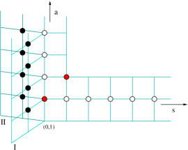
Figure 7: Domain of definition of the T-system (259)-(261). In our notations, T functions belonging to the two wings of the diagram are distinguished by the superscript $\alpha\in\left\{I,II\right\}$.

They are expressed in terms of two special gauges, denoted as ${\bf T}$ and ${\mathbb{T}}$. The properties of the $\bf{T}$ gauge needed in the following derivation are:

(i)

Analyticity strips: denoting as $\mathcal{A}_{n}$ the class of functions free of branch point singularities in the strip $|\text{Im}(u)|<\frac{n}{2}$, we have

$$({\bf T}_{n,0}^{\alpha})\in\mathcal{A}_{n+1},\hskip 14.22636pt({\bf T}_{n,1})\in\mathcal{A}_{n},\hskip 14.22636pt({\bf T}_{n,2})\in\mathcal{A}_{n-1},\hskip 14.22636ptn\in\mathbb{N},\;\;\;\alpha\in\left\{I,II\right\}.$$ (263)

Besides, on the leftmost edges of the diagram: ${\bf T}_{n,-1}^{\alpha}=1$.

(ii)

The two functions ${\bf T}_{0,0}^{I}$, ${\bf T}_{0,0}^{II}$ are equal, and periodic on the mirror section:

$$({\bf T}_{0,0}^{I})^{(+1)}(u) = ({\bf T}_{0,0}^{II})^{(+1)}(u)\equiv\check{\mu}_{12},$$ (264)

$$\check{\mu}_{12}^{(+1)} = \check{\mu}_{12}^{(-1)}.$$ (265)

The function $\check{\mu}_{12}$ defined above will eventually be identified with an element of the $\mu_{AB}$ matrix appearing in the QSC equations. The notation $\check{\mu}_{12}$ signals that, throughout this Appendix, we will consider $\check{\mu}_{12}(u)$ as a function defined on the mirror Riemann section with long cuts, where it is $i$-periodic. This function agrees with $\mu_{12}(u)$ used in the rest of the paper in the strip $0<\text{Im}(u)<1/2$, and elsewhere is obtained by analytic continuation keeping all cuts long. Notice that the mirror $i$-periodicity of $\check{\mu}(u)$ is equivalent to the property (15).

(iii)

Finally, the $\bf{T}$ functions enjoy the following group-theoretical properties:

$${\bf T}_{0,n}=(\check{\mu}_{12}^{(n)})^{2},\hskip 28.45274pt{\bf T}_{n+1,2}={\bf T}_{2,n+1},\hskip 56.9055ptn\in\mathbb{N}^{+}.$$ (266)

We expect that the ${\bf T}$ gauge defined by these properties is essentially unique (apart from rescalings by constants independent of $u$). The $\mathbb{T}$ gauge may be defined by a transformation:

$${\bf T}_{n,s}(u) ={\mathbb{T}}_{n,s}(u)\left(\check{\mu}_{12}^{(n+s-1)}(u)\right)^{2-n}, s\in\mathbb{N}^{+},\;n\in\mathbb{N},$$ (267)

$${\bf T}_{n,0}^{\alpha}(u) ={\mathbb{T}}_{n,0}^{\alpha}(u)\,\left(\sqrt{\check{\mu}_{12}^{(n-1)}(u)}\right)^{2-n}\;(d^{(n)}(u))^{s_{\alpha}\,n},\;\; \alpha\in\left\{I,II\right\},\;n\in\mathbb{N}$$ (268)

$${\bf T}_{n,-1}^{\alpha}(u) ={\mathbb{T}}_{n,-1}^{\alpha}(u)=1, \alpha\in\left\{I,II\right\},\;n\in\mathbb{N},$$ (269)

where $s_{I}=-s_{II}=+1$, and $d(u)=d^{(+2)}(u)$ is a mirror $i$-periodic function, representing an additional degree of freedom in the definition which will be practically irrelevant for our derivation. It is simple to check that (267)-(269) leave invariant the form of the T-system due to the mirror periodicity of $\check{\mu}_{12}$ and $d(u)$.

In general, we expect both the ${\bf T}$ and ${\mathbb{T}}$ functions to exhibit an infinite ladder of branch points for $u\in\pm 2h+i\mathbb{Z}/2$. From the TBA analysis, we know that these singularities are all of square-root type and that analytic continuation around branch points symmetric with respect to the imaginary axis leads to the same sheets. This structure is further specified by the property $\bf{(i)}$ above: some of the potential branch points in the ${\bf T}$ functions fall inside the analyticity strips and therefore they must have trivial monodromy.

Besides, the ${\mathbb{T}}$ functions enjoy some special properties when continued to the short-cut section of the Riemann surface (also known as the physical sheet). We will denote their values on this section as $\hat{\mathbb{T}}$: in analogy with the case of $\check{\mu}$ and $\mu$, the convention is that ${\mathbb{T}}$ and $\hat{{\mathbb{T}}}$ are the same in the analyticity strip immediately above the real axis, while in the rest of the complex plane, they are defined by analytic continuation keeping long cuts for ${\mathbb{T}}$ and short cuts for $\hat{{\mathbb{T}}}$. The $\hat{{\mathbb{T}}}_{a,s}$ functions have the following nontrivial properties:

(a)

the functions $\hat{\mathbb{T}}_{1,n}$ with $n\geq 1$ have only two short branch cuts: $(-2h,2h)\pm in/2$,

(b)

the functions $\hat{\mathbb{T}}_{2,m}$ with $m\geq 2$ have only four short branch cuts, lying at $(-2h,2h)\pm i(m-1)/2$, $(-2h,2h)\pm i(m+1)/2$.

The goal of the following derivation is to obtain the Riemann-Hilbert type equations characterizing the QSC. We will see that the whole structure can be derived by imposing the consistency of the conditions (i), (ii) , (iii) and (a), (b).

Let us make an additional comment. Here, we do not aim to derive the regularity properties of the QSC, namely the statement that ${\bf P}(u)$ and $\nu(u)$ functions are entire on the Riemann surface defined by the branch points at $u\in\pm 2h\pm i\mathbb{Z}$. However, it is natural to expect that this condition is equivalent to the requirement that the T functions are regular in appropriate gauges, and indeed one can verify a posteriori that, picking appropriately the function $d(u)$ in (267) and assuming the regularity of the QSC, all the ${\bf T}$ and ${\mathbb{T}}$ functions can be chosen to be regular. For instance, it is possible to identify ${\bf T}_{1,0}^{I}(u)=\nu_{1}(u)\,\widetilde{\nu}_{1}(u)$, ${\bf T}_{1,0}^{II}(u)=\nu^{4}(u)\,\widetilde{\nu}^{4}(u)$. Therefore, choosing $d(u)\propto(\nu_{1}(u)/\nu^{4}(u))^{\frac{1}{2}}$, one can set ${\mathbb{T}}_{1,0}^{I}(u)\propto\widetilde{\nu}_{1}(u)$, ${\mathbb{T}}_{1,0}^{II}(u)\propto\widetilde{\nu}^{4}(u)$, from which we have a clear indication that the regularity properties of the $\nu$ and T functions are equivalent. This example also illustrates the fact that a requirement of regularity for the ${\mathbb{T}}$ gauge specifies the function $d(u)$ uniquely, apart for an overall constant. However, we remark that, for the purposes of the following derivation, the precise form of $d(u)$ is irrelevant: this function cancels out of all the equations reported below.

A.2 Strategy of the derivation

The main tactic of the derivation is to choose a parametrization of the ${\mathbb{T}}$ functions that makes (a), (b) explicit; we will then reconstruct the ${\bf T}$ functions through (267) and impose the validity of (i), (ii), (iii).

To start, we notice that the properties (a), (b) presented above can be encapsulated by the following parametrization (see Section 4.2 in FiNLIE ):

$$\hat{{\mathbb{T}}}_{1,s} = {\bf P}_{1}^{\left[+s\right]}{\bf P}_{2}^{\left[-s\right]}-{\bf P}_{2}^{\left[+s\right]}{\bf P}_{1}^{\left[-s\right]},\;\;\;,\;\;\;\;\hat{{\mathbb{T}}}_{2,s+1}=\hat{{\mathbb{T}}}_{1,1}^{\left[+s+1\right]}\hat{{\mathbb{T}}}_{1,1}^{\left[-s-1\right]},\;\;s\in\mathbb{N}^{+},$$ (270)

$$\hat{{\mathbb{T}}}_{0,0}^{\alpha} = 1,\;\;\;,\;\;\;\;\hat{{\mathbb{T}}}_{0,s}=1,\;\;s\in\mathbb{N}^{+},\;\;\alpha\in\left\{I,II\right\},$$ (271)

where ${\bf P}_{1}$, ${\bf P}_{2}$ are functions with a single short cut. Notice that this parametrization covers only the right tail of the T-hook diagram. To reach the rest of the diagram using the T-system relation (259), we need one more constraint involving at least one node outside this domain. For this purpose we may use

$$\mathbb{T}_{3,2}/\mathbb{T}_{2,3}=\check{\mu}_{12},$$ (272)

which follows from the transformation (267) combined with the property (iii). We then see that, applying Hirota equation starting from any point in the right band, we may parametrize any of the ${\mathbb{T}}$ functions in terms of only three building blocks, the functions ${\bf P}_{1}$, ${\bf P}_{2}$, $\mu_{12}$, which as we will see will be evaluated on various Riemann sheets. The $\bf{T}$ functions, defined through (267), can be expressed in terms of the same data, and one can check that they satisfy the constraints (ii), (iii) by construction. However, it is not obvious that they have the correct analyticity strips described by condition (i); we still need to impose an infinite ladder of relations:

$$\triangle\left(({\bf T}_{n+1,0}^{\alpha})^{(+n)}\right)=\triangle\,\left({\bf T}_{n+2,1}^{(+n)}\right)=0,$$ (273)

where we use the symbol $\triangle$ for the discontinuity $\triangle f\equiv f-\tilde{f}$ expressing the monodromy around any of the branch points at $\pm 2h$ on the real axis. The conditions (273) place further constraints on ${\bf P}_{1}$, ${\bf P}_{2}$ and $\check{\mu}_{12}$ and will lead us to the QSC equations.

As a convenient notation, we will introduce a splitting function $g(u)$, defined through

$$g^{2}\equiv\frac{{\bf T}_{1,0}^{I}}{{\bf T}_{1,0}^{II}}=\frac{{\mathbb{T}}_{1,0}^{I}}{{\mathbb{T}}_{1,0}^{II}}\,d^{2}.$$ (274)

In particular, in the $4\leftrightarrow\bar{4}$-symmetric subsector in which ${\bf T}_{n,0}^{I}={\bf T}_{n,0}^{II}$, one has simply $g(u)=1$.

A.3 Details

Before discussing the derivation in detail, let us mention a technical point. In the following paragraphs, we will find relations between functions which are defined, by default, on different sections of the Riemann surface covering the $u$ plane. To remove possible ambiguities, we specify that all the equations below are valid for $u$ in a strip slightly above the real axis. With this understanding, we will use interchangeably $\check{\mu}_{12}$ and $\mu_{12}$ in the following equations.

First level $n=0$

The first constraint coming from (273) is that ${\bf T}_{2,1}={\mathbb{T}}_{2,1}$ has no cut on the real axis. The consequences of this requirement were already discussed in Cavaglia:2014exa . Using Hirota equation and carefully continuing the expressions (270) to the mirror sheet, we find

$$\mathbb{T}_{2,1} = \frac{{\mathbb{T}}_{2,2}^{(+1)}\,{\mathbb{T}}_{2,2}^{(-1)}-\mathbb{T}_{1,2}\mathbb{T}_{32}}{\mathbb{T}_{23}}$$ (275)

$$= ({\bf P}_{1}^{[+2]}{\bf P}_{2}-{\bf P}_{2}^{[+2]}{\bf P}_{1})({\widetilde{\bf P}}_{1}{\bf P}_{2}^{[-2]}-{\widetilde{\bf P}}_{2}{\bf P}_{1}^{[-2]})-{\mu}_{12}\,\mathbb{T}_{1,2}.$$ (276)

Imposing the absence of a cut on the real axis, we obtain

$$\triangle\left(\mathbb{T}_{2,1}\right)={\mathbb{T}}_{1,2}\,\left({\widetilde{\mu}}_{12}-\mu_{12}-{\bf P}_{1}{\widetilde{\bf P}}_{2}+{\bf P}_{2}{\widetilde{\bf P}}_{1}\right)=0,$$ (277)

and, since $\mathbb{T}_{1,2}$ cannot be zero everywhere, we get a first relation of the ${\bf P}\mu$-system (16):

$$\mu_{12}+{\bf P}_{1}\,{\widetilde{\bf P}}_{2}-{\bf P}_{2}{\widetilde{\bf P}}_{1}={\widetilde{\mu}}_{12}.$$ (278)

Using the Hirota equation centered at the node $(1,1)$, we can also compute

$${\bf T}_{1,0}^{I}\,{\bf T}_{1,0}^{II}=\mu_{12}\,\frac{{{\mathbb{T}}}_{1,1}^{(+1)}\,{{\mathbb{T}}}_{1,1}^{(-1)}-{\mathbb{T}}_{2,1}}{{\mathbb{T}}_{1,2}}=\mu_{12}\,(\mu_{12}+{\bf P}_{1}{\widetilde{\bf P}}_{2}-{\bf P}_{2}{\widetilde{\bf P}}_{1})=\mu_{12}\,\widetilde{\mu}_{12},$$ (279)

which means we can parametrize

$${\bf T}_{1,0}^{I}(u)=\sqrt{\mu_{12}(u)\widetilde{\mu}_{12}(u)}\,g(u),\;\;\;\;\;{\bf T}_{1,0}^{II}(u)=\frac{\sqrt{\mu_{12}(u)\widetilde{\mu}_{12}(u)}}{g(u)}.$$ (280)

The requirement that ${\bf T}_{1,0}^{\alpha}$ have no cuts on the real axis then imposes $\triangle(g(u))=0$.

General level

As illustrated in the previous example, the functions ${\mathbb{T}}_{a,s}$ with $a>s$, computed using the T-system relations, will depend not only on the values of ${\bf P}_{1}$, ${\bf P}_{2}$ and $\mu_{12}$ on their defining sheet, but also on their shifted values on the second sheet: this is due to the fact that Hirota equation is defined on the mirror section, while the cut in the definition of ${\bf P}_{1}$ and ${\bf P}_{2}$ is short. In general, the constraints (273) can be translated as conditions on the monodromies of $\widetilde{{\bf P}}_{1}$, $\widetilde{{\bf P}}_{2}$ and $g$ around the branch points lying further and further from the real axis. Remarkably, the content of (273) can be recast in a very simple form: the constraints on the cuts in the upper half plane yield

$$\mu_{12}\,\widetilde{(\widetilde{\bf P}_{A})^{(2n)}}=+{\bf P}_{1}^{(2n)}\,\triangle({\bf P}_{2}\,{\bf P}_{A})-{\bf P}_{2}^{(2n)}\,\triangle({\bf P}_{1}\,{\bf P}_{A})+(\widetilde{\bf P}_{A})^{(2n)}\,\widetilde{\mu}_{12}+2\,\triangle({\bf P}_{A})\,\eta_{n},$$ (281)

for $n\in\mathbb{N}^{+}$, $A\in\left\{1,2\right\}$, with

$$\eta_{n}\equiv\frac{1}{2}\left(\frac{g^{(+2n)}}{g}+\frac{g}{g^{(+2n)}}\right)\,\sqrt{\widetilde{\mu}_{12}\;(\widetilde{\mu}_{12})^{(2n)}}+\widetilde{\bf P}_{1}{\bf P}_{2}^{(2n)}-\widetilde{\bf P}_{2}{\bf P}_{1}^{(2n)},$$ (282)

together with the condition that

$$\triangle{\Big{(}}\frac{g^{(+2n)}}{g}\;\sqrt{\frac{(\widetilde{\mu}_{12})^{(2n)}}{\mu_{12}}}{\Big{)}}=\triangle{\Big{(}}\frac{g}{g^{(+2n)}}\;\sqrt{\frac{(\widetilde{\mu}_{12})^{(2n)}}{\mu_{12}}}{\Big{)}}.$$ (283)

One obtains very similar but not identical equations describing the discontinuities in the lower half plane. For conciseness, we will only refer to (281) in the following arguments. Remarkably, the form of these relations contains already the full structure of the QSC.

Constructing the ${\bf P}\mu$-system

The equations in (281) can be rewritten as

$$-{\tilde{\mu}}_{12}\mu_{12}\;\triangle{\Big{(}}\frac{\widetilde{\bf P}_{A}^{(2n)}}{\mu_{12}}{\Big{)}}=+{\bf P}_{1}^{(2n)}\,\triangle({\bf P}_{2}\,{\bf P}_{A})-{\bf P}_{2}^{(2n)}\,\triangle({\bf P}_{1}\,{\bf P}_{A})+2\,\triangle({\bf P}_{A})\,\eta_{n},$$ (284)

for $A\in\left\{1,2\right\}$. Considering the discontinuity of these relations on the real axis, we see that $\triangle(\eta_{n})=0$. Inspecting expression (282), we then see that

$$\frac{{\Big{(}}-{\bf P}_{1}^{(+2n)}\triangle({\bf P}_{2})+{\bf P}_{2}^{(+2n)}\,\triangle({\bf P}_{1}){\Big{)}}}{\sqrt{\widetilde{\mu}_{12}\,\mu_{12}}}=\triangle{\Big{(}}\frac{g_{\alpha}^{(+2n)}}{g_{\alpha}}\;\sqrt{\frac{(\widetilde{\mu}_{12})^{(2n)}}{\mu_{12}}}{\Big{)}},\;\;\;\alpha\in\left\{I,II\right\},$$ (285)

with $g_{I}=g$, $g_{II}=1/g$. We will exploit (285) to construct two new functions with a single short cut, which we denote as ${\bf P}_{5}$ and ${\bf P}_{6}$ in anticipation of their role in the QSC equations. They are defined through

$${\bf P}_{5}\equiv\frac{\sqrt{\widetilde{\mu}_{12}}}{\sqrt{\mu_{12}}}\;g-{\bf P}_{2}\,\phi_{1,I}+{\bf P}_{1}\,\phi_{2,I},\;\;\;\;\;{\bf P}_{6}\equiv\frac{\sqrt{\widetilde{\mu}_{12}}}{\sqrt{\mu_{12}}\;g}-{\bf P}_{2}\,\phi_{1,II}+{\bf P}_{1}\,\phi_{2,II},$$ (286)

where the functions $\phi_{A,\alpha}$, with indices $A\in\left\{1,2\right\}$, $\alpha\in\left\{I,II\right\}$, are defined from the requirement that they are periodic on the mirror section, with power-like asymptotics and with discontinuities

$$\sqrt{\widetilde{\mu}_{12}\mu_{12}}\;\triangle(\phi_{A,\alpha})=\triangle({\bf P}_{A})\,g_{\alpha},\;\;\;\;A\in\left\{1,2\right\},\;\;\alpha\in\left\{I,II\right\}.$$ (287)

Combining (287) and (286), we can indeed verify that the newly constructed functions have vanishing discontinuities in the upper half plane $\triangle({\bf P}_{5}^{(+2n)})=\triangle({\bf P}_{6}^{(+2n)})=0$, $\forall n\in\mathbb{N}^{+}$. A simple extension of this analysis shows that (286) defines a function with only a single short cut on the real axis.

Let us point out that, when $g=1$ (which is appropriate for $4\leftrightarrow\bar{4}$-symmetric states), by definition we have ${\bf P}_{5}={\bf P}_{6}$, in agreement with the rules described in Section 4.4. As another side remark, notice that the definitions (286) can be recognized as two equations of the ${\bf P}\nu$-system (32) provided the mirror-periodic functions $\phi_{A,\alpha}$ are identified as ratios of $\nu$ functions, and $g(u)$ is identified as

$$g^{2}=\frac{\nu_{1}\,\widetilde{\nu}_{1}}{\nu^{4}\,\widetilde{\nu}^{4}}.$$ (288)

In the rest of this Appendix, for simplicity we will concentrate solely on obtaining the “${\bf P}\mu$” vector form of the equations.

Using (286),(282), equations (284) becomes

$$-{\widetilde{\mu}}_{12}\mu_{12}\;\triangle{\Big{(}}\frac{\widetilde{\bf P}_{{A}}^{(2n)}}{\mu_{12}}{\Big{)}} = +{\bf P}_{1}^{(2n)}\left[\triangle({\bf P}_{{A}}\,{\bf P}_{2})-2\,\triangle({\bf P}_{{A}})\,\left({\widetilde{\bf P}}_{2}+\sqrt{{\widetilde{\mu}}_{12}\mu_{12}}\sum_{\alpha=I,II}\frac{\phi_{2,\alpha}}{2g_{\alpha}}\right)\right]$$ (289)

$$-{\bf P}_{2}^{(2n)}\left[\triangle({\bf P}_{1}\,{\bf P}_{{A}})-2\,\triangle({\bf P}_{{A}})\,\left({\widetilde{\bf P}}_{1}+\sqrt{{\widetilde{\mu}}_{12}\mu_{12}}\sum_{\alpha=I,II}\frac{\phi_{1,\alpha}}{2g_{\alpha}}\right)\right]$$

$$+\triangle({\bf P}_{{A}})\,\left({{\bf P}_{5}}^{(2n)}\,\frac{\sqrt{\widetilde{\mu}_{12}\mu_{12}}}{g}+{\bf P}_{6}^{(2n)}\,g\;\sqrt{\widetilde{\mu}_{12}\mu_{12}}\right),$$

with $A\in\left\{1,2\right\}$. Let us now introduce four functions $\Phi_{AB}$, periodic on the mirror sheet, $\Phi_{AB}=\Phi_{AB}^{(+2n)}$, for $A,B\in\left\{1,2\right\}$, whose (periodically repeated) discontinuities are

$${\mu_{12}\widetilde{\mu}_{12}}\,\triangle(\Phi_{AB})=\triangle({\bf P}_{A}{\bf P}_{B})-2\,\triangle({\bf P}_{A})\,\left({\widetilde{\bf P}}_{B}+\sqrt{{\widetilde{\mu}}_{12}\mu_{12}}\sum_{\alpha=I,II}\frac{\phi_{B,\alpha}}{2g_{\alpha}}\right).$$ (290)

Then, defining the functions ${\bf P}_{3}$ and ${\bf P}_{4}$ as

$$-{\bf P}_{3} \equiv \frac{\widetilde{\bf P}_{1}}{\mu_{12}}+\Phi_{12}\,{\bf P}_{1}-\Phi_{11}\,{\bf P}_{2}+{\phi}_{1,II}\,{\bf P}_{5}+\phi_{1,I}\,{\bf P}_{6},$$ (291)

$$-{\bf P}_{4} \equiv \frac{\widetilde{\bf P}_{2}}{\mu_{12}}+\Phi_{22}\,{\bf P}_{1}-\Phi_{21}\,{\bf P}_{2}+{\phi}_{2,II}\,{\bf P}_{5}+\phi_{2,I}\,{\bf P}_{6},$$ (292)

we see that, due to (289),

$$\triangle({\bf P}_{3}^{(2n)})=\triangle({\bf P}_{4}^{(2n)})=0,\;\;\;\;\;n\in\mathbb{N}^{+},$$ (293)

therefore ${\bf P}_{3}$ and ${\bf P}_{4}$ are free of branch points in the upper half plane and, by a small additional effort, we can show that they have just a single short cut on the real axis.

Let us summarize the situation: by a scrutiny of the equations, we have so far found six functions with a single short cut, and eight mirror-periodic functions $\Phi_{AB}$ , $\phi_{A,\alpha}$. It remains only to check that the relations between their monodromies can be written in a closed form.

The fifteen components of the antisymmetric matrix $\mu_{AB}$ can be defined in terms of the periodic functions introduced above. Indeed, setting

$$\mu_{14}=-\Phi_{12}\,\mu_{12}-1,\quad\mu_{13}=-\Phi_{11}\,\mu_{12},\quad\mu_{15}=-\phi_{1,I}\,\mu_{12},\quad\mu_{16}=-{\phi}_{1,II}\,\mu_{12},$$ (294)

$$\mu_{24}=-\Phi_{22}\,\mu_{12},\quad\mu_{23}=-\Phi_{21}\,\mu_{12}+1,\quad\mu_{25}=-\phi_{2,I}\,\mu_{12},\quad\mu_{26}=-{\phi}_{2,II}\,\mu_{12},$$ (295)

we immediately recognize that (291),(292) are two equations of the ${\bf P}\mu$-system. Besides, the form of these relations implies the existence of three quadratic constraints among the matrix elements defined in (294); let us discuss in detail how these conditions emerge. Consider the following equation:

$$\mu_{13}-\widetilde{\mu}_{13}+{\bf P}_{1}\widetilde{\bf P}_{3}-{\bf P}_{3}\widetilde{\bf P}_{1}=-2\,(\mu_{12}-\widetilde{\mu}_{12})\,(\Phi_{11}-\phi_{1,I}\,\phi_{1,II}),$$ (296)

which can be derived from (291) and its analytic continuation to the second sheet using the monodromy rules (278),(287),(290). The form of (296) implies that the combination of mirror-periodic functions $\Phi_{11}-\phi_{1,I}\,\phi_{1,II}$ must be free of cuts. Due to its power-like asymptotics, it must be a constant independent of $u$ and, using the freedom to redefine the $\Phi$’s by a constant shift, we will assume that $\Phi_{11}-\phi_{1,I}\,\phi_{1,II}=0$. Therefore, (296) can be recognized as another equation of the ${\bf P}\mu$-system. Moreover, the quadratic constraint we have just found can be rewritten as $\mu_{12}\mu_{13}-\mu_{15}\mu_{16}=0$, which is one of the components of the matrix equation $(\mu\eta)^{2}=0$. By similar reasoning, we can impose two more constraints and all in all we can set

$$\Phi_{11}-\phi_{1,I}\,\phi_{1,II}=0,\;\;\;\;\;\Phi_{22}-\phi_{2,I}\,\phi_{2,II}=0,\;\;\;\;\;\Phi_{12}+\Phi_{21}+\phi_{1,I}\phi_{2,II}+\phi_{2,I}\phi_{1,II}=0.$$ (297)

The rest of the derivation goes along the same lines. The remaining independent entries of $\mu_{AB}$ are defined as:

$$\mu_{35}=\phi_{1,I}\,(\mu_{23}-\mu_{12}\,{\phi}_{1,II}\,\phi_{2,I}),\quad\mu_{36}={\phi}_{1,II}\,(\mu_{23}-\mu_{12}\,{\phi}_{1,I}\,\phi_{2,II}),$$ (298)

$$\mu_{45}=\phi_{2,I}\,(\mu_{23}-\mu_{12}\,{\phi}_{1,II}\,\phi_{2,I}),\quad\mu_{46}={\phi}_{2,II}\,(\mu_{23}-\mu_{12}\,{\phi}_{1,I}\,\phi_{2,II}),$$ (299)

$$\quad\mu_{34}=\frac{\mu_{35}\,\mu_{36}}{\mu_{12}\,\phi_{1,I}\,{\phi}_{1,II}},\quad\mu_{56}=-\mu_{12}({\phi}_{1,II}\,\phi_{2,I}-\phi_{1,I}\,{\phi}_{2,II}),$$ (300)

and it is possible to verify that all equations of the ${\bf P}\mu$ system, including the quadratic constraints on the ${\bf P}$ and $\mu$ functions, follow from the relations listed above (and their analytic continuation through the branch cut on the real axis).

The specific form of the matrix $\eta_{AB}$ entering the ${\bf P}\mu$-system equations does depend on the normalization of our definitions (286),(291),(292),(294)-(300), and could be changed by rescaling some of the $\mu$ or ${\bf P}$ functions, or by a more general linear change of basis, ${\bf P}_{A}(u)\rightarrow H_{A}^{B}\,{\bf P}_{B}(u)$, $\mu_{AB}(u)\rightarrow H_{A}^{C}\,H_{B}^{D}\,\mu_{CD}(u)$, which would transform $\eta_{AB}\rightarrow H_{A}^{C}\,H_{B}^{D}\,\eta_{CD}$. However, $\eta_{AB}$ is clearly always a symmetric tensor, and besides its signature $(+++---)$ is invariant under all linear transformations with $H\in\mathbb{R}^{6\times 6}$. This reality restriction is meaningful since it preserves the following property: for real values of the coupling, all the functions ${\bf P}_{A}(u)$ can be chosen to be real on the Riemann section with short cuts. This property is verified with our choice of conventions, and follows from the reality of the solutions of the TBA.

Appendix B Algebraic identities

B.1 Identities for gamma matrices

In this Appendix we collect some useful algebraic identities, descending from the properties of gamma and sigma matrices for $SO(3,3)$ and $SO(3,2)$. The defining relation for the $SO(3,3)$ sigma matrices is

$$(\sigma_{A})_{ac}\;(\bar{\sigma}_{B})^{cb}+(\sigma_{B})_{ac}\;(\bar{\sigma}_{A})^{cb}=\delta_{a}^{b}\;\eta_{AB},$$ (301)

and we recall that $(\sigma_{AB})_{a}^{b}$ is defined through

$$(\sigma_{A})_{ac}\;(\bar{\sigma}_{B})^{cb}-(\sigma_{B})_{ac}\;(\bar{\sigma}_{A})^{cb}=-2\;(\sigma_{AB})_{a}^{b},$$ (302)

so that we have

$$(\sigma_{A})_{ac}\;(\bar{\sigma}_{B})^{cb}=\frac{1}{2}\,\delta_{a}^{b}\;\eta_{AB}-(\sigma_{AB})_{a}^{b}.$$ (303)

A useful property, specific to orthogonal groups in six and five dimensions, is the fact that gamma matrices are anti-symmetric: $(\sigma_{A})_{ab}=-(\sigma_{A})_{ba}$. This allows us to prove the following very useful relation:

$$\left(\bar{\sigma}_{C}\,\sigma_{A}\,\bar{\sigma}_{B}-\bar{\sigma}_{C}\,\sigma_{B}\,\bar{\sigma}_{A}\right)^{ab}=\eta_{AC}\,(\bar{\sigma}_{B})^{ab}-\eta_{BC}\,(\bar{\sigma}_{A})^{ab},$$ (304)

and its consequence

$$\text{Tr}\left(\sigma_{AB}\,\sigma^{CD}\right)=\delta_{A}^{D}\,\delta_{B}^{C}-\delta_{A}^{C}\,\delta_{B}^{D}.$$ (305)

Another identity that is specific to this dimension is

$$\bar{\sigma}^{ab}=-\frac{1}{2}\,\epsilon^{abcd}\,\sigma_{cd},$$ (306)

which implies in particular that $(\sigma_{AB})$ is traceless: $(\sigma_{AB})_{a}^{a}=0$, and moreover that, for any anti-symmetric matrix $4\times 4$ matrix $G_{ab}$:

$$2\,\text{Pf}(G_{ab})=G_{A}\,\eta^{AB}\,G_{B},$$ (307)

where the corresponding vector $\left\{G_{A}\right\}_{A=1}^{6}$ is defined by $G_{ab}=G_{A}\,(\sigma^{A})_{ab}$. Another useful formula is:

$$(\sigma_{A})_{ab}(\bar{\sigma}_{B})^{cd}-(\sigma_{B})_{ab}(\bar{\sigma}_{A})^{cd}=(\sigma_{AB})^{c}_{a}\,\delta^{d}_{b}-(\sigma_{AB})^{c}_{b}\,\delta^{d}_{a}-(\sigma_{AB})^{d}_{a}\,\delta^{c}_{b}+(\sigma_{AB})^{d}_{b}\,\delta^{c}_{a}.$$ (308)

All the properties listed above are independent on for any choice of chiral representation of the gamma matrices. The situation is analogous for the representations of $SO(3,2)$. In that case we recall that we use the symbols $(\Sigma_{I})_{ij}$, $(\Sigma_{IJ})_{i}^{j}$, and denote the metric as $\rho_{IJ}\equiv\frac{1}{2}\,\text{Tr}(\Sigma_{I}\,\bar{\Sigma}_{J})$. In particular the defining relation for the matrices $\Sigma_{I}$ and $\Sigma_{IJ}$ is:

$$(\Sigma_{I})_{ki}\;(\bar{\Sigma}_{J})^{il}=\frac{1}{2}\,\delta_{k}^{l}\;\rho_{IJ}-(\Sigma_{IJ})_{k}^{l},$$ (309)

with $\Sigma_{IJ}=-\Sigma_{JI}$. On top of these properties, in the $SO(3,2)$ case the matrices $\Sigma$ and $\bar{\Sigma}$ are related by a similarity transformation:

$$(\Sigma_{I})_{ij}=\left(\kappa_{ik}\,(\bar{\Sigma}_{I})^{kl}\,\kappa_{lj}\right),$$ (310)

where $\kappa_{ij}$ is an anti-symmetric $4\times 4$ matrix. Equation (310) can be used to prove the additional symmetry property $(\Sigma_{IJ})_{ij}=+(\Sigma_{IJ})_{ji}$. Finally, the analogue of (305), (304) are

$$\text{Tr}\left(\Sigma_{IJ}\,\Sigma^{KL}\right) = \delta_{I}^{L}\,\delta_{J}^{K}-\delta_{I}^{K}\,\delta_{J}^{L},$$ (311)

$$\left(\bar{\Sigma}_{K}\,\Sigma_{I}\,\bar{\Sigma}_{J}-\bar{\Sigma}_{K}\,\Sigma_{J}\,\bar{\Sigma}_{I}\right)^{ij} = \rho_{IK}\,(\bar{\Sigma}_{J})^{ij}-\rho_{JK}\,(\bar{\Sigma}_{I})^{ij}.$$ (312)

Finally, we report below some useful identities for a generic antisymmetric $4\times 4$ matrix $G_{ab}=-G_{ba}$:

$$G_{ab}\,G_{cd}-G_{cb}\,G_{ad}-G_{ac}\,G_{bd} = \epsilon_{abcd}\,\text{Pf}(G),$$ (313)

$$-\frac{1}{2}\,\epsilon^{ijkl}\,G_{kl}\,G_{jm} = \delta_{m}^{i}\;\text{Pf}(G),$$ (314)

$$G_{ik}\;G_{jl}\;\epsilon^{klmn} = -\text{Pf}(G)\;\left(G_{ij}\;G^{mn}+\delta_{i}^{m}\,\delta_{j}^{n}-\delta_{i}^{n}\,\delta_{j}^{m}\right),$$ (315)

$$G_{ij}=-\frac{1}{2}\,\epsilon_{ijkl}\,G^{kl}\,\text{Pf}(G),$$ (316)

where we recall that the Pfaffian is defined as

$$\text{Pf}(G)=\frac{1}{8}\,\epsilon^{abcd}\,G_{ab}\,G_{cd}=G_{12}G_{34}+G_{14}G_{23}-G_{13}G_{24}.$$ (317)

In particular:

$$\kappa_{ik}\;\kappa_{jl}\;\epsilon^{klmn}=\left(\kappa_{ij}\;\kappa^{mn}+\delta_{i}^{m}\,\delta_{j}^{n}-\delta_{i}^{n}\,\delta_{j}^{m}\right).$$ (318)

B.2 Relation between $Q_{ab|ij}$ and $Q^{ab}_{\,|ij}$

In Section 7.1, we have defined the objects $Q_{ab|ij}$ as subdeterminants of the $4\times 4$ matrix $\left\{Q_{a|i}\right\}$. Notice that, in principle, one can also define

$$Q^{ab}_{\,|ij}=Q^{a}_{\,|i}\,Q^{b}_{\,|j}-Q^{a}_{\,|j}\,Q^{b}_{\,|i}.$$ (319)

However, a simple linear algebra identity relates the minors of a matrix and its inverse, and shows that the two definitions are algebraically related:

$$Q_{ab|ij}=\frac{1}{2}\,\left(\text{det}(Q_{\ast|\ast})\right)\,\epsilon_{abcd}\;\epsilon_{ijkl}\;Q^{c|k}\,Q^{d|l}=-\frac{1}{2}\,\epsilon_{abcd}\;\epsilon_{ijkl}\;Q^{c|k}\,Q^{d|l}.$$ (320)

From (320), we see that

$$Q_{ab|ij}=-\frac{1}{2}\,\epsilon_{abcd}\,Q^{c}_{\,|j_{1}}\,Q^{d}_{\,|j_{2}}\,\epsilon_{ijkl}\,\kappa^{kj_{1}}\,\kappa^{lj_{2}},$$ (321)

and using (318) we find

$$Q_{ab|ij}=-\frac{1}{2}\,\epsilon_{abcd}\;\left(Q^{cd}_{\,|ij}+\kappa_{ij}\;Q^{cd}_{\circ}\right).$$ (322)

Let us define the projections:

$$Q_{ab|\circ}\equiv\frac{1}{2}Q_{ab|ij}\,\kappa^{ij},\;\;\;\;\;\;Q_{ab|\overline{(ij)}}\equiv Q_{ab|ij}+\frac{1}{2}\kappa_{ij}\,Q_{ab|\circ},$$ (323)

where $Q_{ab|\overline{(ij)}}$ denotes the traceless part and satisfies $Q_{ab|\overline{(ij)}}\,\kappa^{ij}=0$. Identity (322) then splits as

$$Q_{ab|\circ}=\frac{1}{2}\,\epsilon_{abcd}\,Q^{cd}_{\,|\circ},\;\;\;\;\;Q_{ab|\overline{(ij)}}=-\frac{1}{2}\,\epsilon_{abcd}\,Q^{cd}_{\,|\overline{(ij)}}.$$ (324)

B.3 Relation between ${\bf Q}_{ij}$ and its inverse

From (316), we have

$${\bf Q}_{ij}=\frac{1}{2}\epsilon_{ijkl}\;{\bf Q}^{kl},$$ (325)

and, using (313), we immediately find

$${{\bf Q}}_{ij}=\kappa_{ii_{1}}\,\kappa_{jj_{1}}\,{\bf Q}^{i_{1}j_{1}}-\frac{1}{2}\,\kappa_{ij}\,\widehat{{\bf Q}}_{\circ},$$ (326)

where

$$\widehat{{\bf Q}}_{\circ}={{\bf Q}}^{mn}\,\kappa_{mn}.$$ (327)

Contracting (326) with $\kappa^{ij}$, we find that in fact $\widehat{{\bf Q}}_{\circ}={{\bf Q}}_{\circ}={\bf Q}_{ij}\,\kappa^{ij}$, so that (326) reduces to equation (52) presented in the main text.

Appendix C Derivation of constraints on large-$u$ asymptotics

Here we derive the constraints (96), (104) on the asymptotics of ${\bf P}$ and ${\bf Q}$ functions using the QQ-relations derived in Section 7. In order to find (96), we start from relation (144). At large $u$, its rhs is given by

$${\bf P}_{A}(u)\,{\bf Q}_{I}(u)\simeq\mathcal{A}_{A}\,\mathcal{B}_{I}u^{\hat{M}_{I}-M_{A}-1}\,,$$ (328)

which constrains the asymptotic behaviour of ${\mathcal{Q}}_{A|I}$ to be

$${\mathcal{Q}}_{A|I}(u)\simeq-i\frac{\mathcal{A}_{A}\mathcal{B}_{I}u^{\hat{M}_{I}-M_{A}}}{\hat{M}_{I}-M_{A}}.$$ (329)

We may now use the following relation, which is a consequence of the Q-system:

$${\bf Q}_{I}=\pm{\bf P}^{A}\,Q_{A|I}^{\pm},$$ (330)

and gives, using the aymptotics (329), the constraint

$$\sum_{A}\frac{\mathcal{A}_{A}\mathcal{A}^{A}}{\hat{M}_{I}-M_{A}}=0,\quad I=1,\dots,5.$$ (331)

These relations, together with the constraint $\text{Pf}\left({\bf P}_{ij}\right)=1$, may be solved for the terms $\mathcal{A}_{A}\,\mathcal{A}^{A}$, giving precisely (96). To derive (104), it will be convenient to use the following equaton, which can be obtained with simple manipulations from the Q-system relations:

$${\bf P}_{A}={\bf Q}^{I}\,Q_{A|I}^{-}+\frac{{\bf Q}_{\circ}Q_{A|\circ}^{-}}{4}.$$ (332)

The large-$u$ asymptotics of ${\bf Q}_{\circ}$ can be fixed using the first constraint in (85), which yields

$${\bf Q}_{\circ}(u)=4+\frac{2\,\mathcal{C}}{u^{2}}+\mathcal{O}\left(\frac{1}{u^{3}}\right),\quad\mathcal{C}=\mathcal{B}_{1}\mathcal{B}_{4}-\mathcal{B}_{2}\mathcal{B}_{3}+\mathcal{B}_{5}^{2}.$$ (333)

We will also need

$${\bf P}_{A}(u)\simeq u^{-M_{A}}\,\left[\mathcal{A}_{A}+\frac{\mathcal{A}_{A}^{sub}}{u}+\mathcal{O}\left(\frac{1}{u^{2}}\right)\right],$$ (334)

and, from (145),

$$Q_{A|\circ}(u)=u^{-M_{A}}\left[\mathcal{A}_{A}+\frac{\mathcal{A}_{A}^{sub}}{u}+\mathcal{O}\left(\frac{1}{u^{2}}\right)\right].$$ (335)

Expanding (332) at NLO, we find, using (333), (334), (335),

$$\sum_{I=1}^{5}\frac{\mathcal{B}^{I}\mathcal{B}_{I}}{\hat{M}_{I}-M_{A}}=\frac{M_{A}}{2},\quad A=1,\dots,6.$$ (336)

The solution of these equations finally yields (104) and fixes the coefficient $\mathcal{C}$ as in (107).

Finally, for the reader’s convenience, we report more explicitly the constraints (96),(104):

$$\mathcal{A}_{1}\mathcal{A}_{4}=\frac{(M_{1}^{2}-\hat{M}_{1}^{2})(M_{1}^{2}-\hat{M}_{2}^{2})}{(M_{1}^{2}-M_{2}^{2})(M_{1}^{2}-M_{5}^{2})},\;\;\;\;\mathcal{A}_{2}\mathcal{A}_{3}=\frac{(M_{2}^{2}-\hat{M}_{1}^{2})(M_{2}^{2}-\hat{M}_{2}^{2})}{(M_{1}^{2}-M_{2}^{2})(M_{2}^{2}-M_{5}^{2})},\;\;\;\;\mathcal{A}_{5}\mathcal{A}_{6}=\frac{(M_{5}^{2}-\hat{M}_{1}^{2})(M_{5}^{2}-\hat{M}_{2}^{2})}{(M_{5}^{2}-M_{1}^{2})(M_{5}^{2}-M_{2}^{2})},$$

$$\mathcal{B}_{1}\mathcal{B}_{4}=\frac{(\hat{M}_{1}^{2}-M_{1}^{2})(\hat{M}_{1}^{2}-M_{2}^{2})(\hat{M}_{1}^{2}-M_{5}^{2})}{4\,\hat{M}_{1}^{2}\,(\hat{M}_{1}^{2}-\hat{M}_{2}^{2})},\;\;\;\;\mathcal{B}_{2}\mathcal{B}_{3}=\frac{(\hat{M}_{2}^{2}-M_{1}^{2})(\hat{M}_{2}^{2}-M_{2}^{2})(\hat{M}_{2}^{2}-M_{5}^{2})}{4\,\hat{M}_{2}^{2}\,(\hat{M}_{1}^{2}-\hat{M}_{2}^{2})},$$

$$\mathcal{B}_{5}^{2}=-\frac{M_{1}^{2}\,M_{2}^{2}\,M_{5}^{2}}{4\,\hat{M}_{1}^{2}\,\hat{M}_{1}^{2}}.$$ (337)

Appendix D Asymptotics and charges: consistency checks at weak coupling

In this Section we show the emergence of a polynomial Bethe Ansatz in the weak coupling limit and use it to match the parameters entering the asymptotics of the QSC with the quantum numbers of the state, proving (95),(97). The discussion presented below may also be useful for developing an analytic weak coupling solution algorithm valid in every sector.

We shall start from the following large-$u$ asymptotics

$${\bf P}_{A}\sim\left(u^{-M_{1}},u^{-M_{2}},u^{M_{2}},u^{M_{1}},u^{-M_{5}},u^{M_{5}}\right),$$ (338)

$${\bf Q}_{I}\sim\left(u^{\hat{M}_{1}-1},u^{\hat{M}_{2}-1},u^{-\hat{M}_{2}-1},u^{-\hat{M}_{1}-1},u^{-1}\right),$$ (339)

where, for the moment, we view the five charges $\left\{M_{1},\,M_{2},\,M_{5}\right\}\in\mathbb{Z}^{3}$, $\left\{\hat{M}_{1},\hat{M}_{2}\right\}\in\mathbb{R}^{2}$ as generic parameters. Choosing a conventional ordering, we assume that, for small real values of the coupling constant, they are ordered as

$$\hat{M}_{1}>\hat{M}_{2}>M_{2}>M_{1}>|M_{5}|.$$ (340)

Since they are not quantized in integers, the charges $\hat{M}_{i}$ will depend on the coupling. We make the further assumption that, as $h\rightarrow 0$, $\hat{M}_{2}$ and $\hat{M}_{1}$ have integer limiting values: $\lim_{h\rightarrow 0^{+}}\hat{M}_{i}\in\mathbb{Z}$, with deviations of order $\mathcal{O}(h^{2})$. This property will play an important role since it implies that the powers in the asymptotics (338) are integer for $h\sim 0$. Therefore, at leading order in $h$ any Q functions which turns out to be free of singularities must reduce to a polynomial function of $u$.

D.1 Generic features of the weak coupling expansion

We now discuss some general features of the weak coupling limit (see also Marboe:2014gma ).

1) Properties of ${\bf P}$ functions:

As $h\rightarrow 0^{+}$, the branch cuts of the QSC shrink to zero size; each of these cuts is in general replaced by a pole.

For a generic Q function analytic in the upper half plane, we may expect a string of poles for $-u\in i\mathbb{N}$ at weak coupling. However, since the ${\bf P}$ functions originally had only a single cut on the first sheet, at each order in the weak coupling expansion they are rational functions of $u$, with no singularities apart for a multiple pole at $u=0$.

Consistently with relations (C), we will choose a normalization so that the ${\bf P}$’s scale like $\mathcal{O}(h^{0})$ at weak coupling: ${\bf P}_{A}(u)={\bf P}_{A}^{(0)}(u)+\mathcal{O}(h^{2})$. Let us now introduce an important parameter: we denote as $\ell$ the order of the strongest pole occurring among all the functions ${\bf P}_{A}^{(0)}(u)$ at $u=0$, and we will write

$${\bf P}_{A}^{(0)}(u)=u^{-\ell}\,p^{\text{pol}}_{A}(u),$$ (341)

where $p^{\text{pol}}_{A}(u)$ are polynomials in $u$. Notice that we must have $\ell\geq M_{1}>0$, since otherwise ${\bf P}_{1}^{(0)}(u)$ would not have decreasing asymptotics at infinity, contradicting (340). We will see eventually that $\ell$ can be identified with the spin chain length entering the Bethe Ansatz equations at weak coupling.

2) Properties of $\nu$ functions:

In the leading approximation at weak coupling all functions $\nu_{a}(u)$, $\nu^{a}(u)$ are necessarily polynomials in $u$. Let us review the argument leading to this conclusion, following Marboe:2014gma . We start noticing that, at finite $h$, the functions

$$\nu_{a}(u)+\widetilde{\nu}_{a}(u),\;\;\;\;\;\frac{\widetilde{\nu}_{a}(u)-\nu_{a}(u)}{\sqrt{u^{2}-4h^{2}}}$$ (342)

do not have cuts on the real axis. Therefore, when expanded at weak coupling these particular combinations of $\nu$ functions should have no pole at $u=0$, at every loop order. Combining this observation with the mirror-periodicity $\widetilde{\nu}_{a}(u)=e^{i\mathcal{P}}\nu_{a}(u+i)$ shows that, at the leading order at weak coupling, $\nu_{a}(u)$ cannot have a pole neither at $u=0$ nor at $u=i$; further, the difference equation (41) shows that these functions cannot have singularities anywhere else. Therefore, at leading order in the weak coupling expansion they must reduce to polynomial functions of $u$.

Studying the large-$u$ asymptotics, we can also deduce that the components of $\nu_{a}(u)$ must have the same scaling at weak coupling. Furthermore, by an appropriate normalization, we can impose that $\nu_{a}$ and $\nu^{a}$ have the same scaling behaviour. Thus, we can write:

$$\nu_{a}(u)=h^{-\ell_{\ast}}\,(\nu_{a}^{(0)}(u)+\mathcal{O}(h^{2})),\;\;\;\;\nu^{a}(u)=h^{-\ell_{\ast}}\,(\nu^{a(0)}(u)+\mathcal{O}(h^{2})),$$ (343)

where $\nu_{a}^{(0)}(u)$, $\nu^{a(0)}(u)$ are polynomials of $u$. We will prove below that $\ell_{\ast}\geq\ell$. We will see that the zeros of the polynomials $\nu_{1}^{(0)}(u+i/2)$, $\nu^{4(0)}(u+i/2)$ can be identified with $4$ and $\bar{4}$-type Bethe roots entering the 2-loop Bethe Ansatz:

$$\nu_{1}^{(0)}(u)\propto\prod_{j=1}^{K_{4}}(u-u^{(0)}_{4,j}-i/2),\;\;\;\;\nu^{4(0)}(u)\propto\prod_{j=1}^{K_{\bar{4}}}(u-u^{(0)}_{\bar{4},j}-i/2).$$ (344)

Finally, let us study the regularity of the combinations (342) at leading order at weak coupling: imposing the absence of a pole at $u=0$ we find the useful equations

$$(\nu_{a}^{(0)}(0)-e^{i\mathcal{P}^{(0)}}\nu_{a}^{(0)}(+i))=(\nu^{b(0)}(0)-e^{-i\mathcal{P}^{(0)}}\nu^{b(0)}(+i))=0,\;\;\;\;\forall a,b,$$ (345)

where $\mathcal{P}^{(0)}=\lim_{h\rightarrow 0}\mathcal{P}$. From (345), we see that

$$e^{i\mathcal{P}}+\mathcal{O}(h^{2})=\frac{\nu_{1}^{(0)}(0)}{\nu_{1}^{(0)}(i)}=\prod_{j=1}^{K_{4}}\left(\frac{u_{4,j}^{(0)}+i/2}{u_{4,j}^{(0)}-i/2}\right)=\text{exp}(i\sum_{j=1}^{K_{4}}p_{4,j})+\mathcal{O}(h^{2}),$$ (346)

which proves the statement anticipated in Section 3.3: at leading order, $\mathcal{P}$ can be identified with the total momentum of a single species of spin chain magnons.

3) Properties of $\widetilde{\bf P}$:

Important information on the weak coupling behaviour of $\widetilde{\bf P}_{A}$ can be obtained studying the properties of the $1/x(u)$ expansion (14), which is valid at finite $h$.

Consider one of the ${\bf P}_{A}$ functions which exhibits a pole of order $\ell$ in $u=0$. In order to be more explicit, we will take this function to be ${\bf P}_{1}(u)$. Write its $1/x$ expansion as:

$${\bf P}_{1}(u)=\sum_{n=M_{1}}^{\infty}\frac{b_{1,n}}{(hx(u))^{n}},$$ (347)

then, taking into account that $x(u)\sim u/h+\mathcal{O}(h)$, we deduce that the coefficients scale as $b_{1,n}\sim\mathcal{O}(h^{0})$ for $n\leq\ell$ at weak coupling, and at the very least $b_{1,n}\sim\mathcal{O}(h^{2})$ for $n>\ell$.

Sending $x(u)\rightarrow\widetilde{x}(u)=1/x(u)$ in (347), we obtain the expansion

$$\widetilde{\bf P}_{1}(u)=\sum_{n=M_{1}}^{\infty}\frac{b_{1,n}\,x^{n}(u)}{(h)^{n}},$$ (348)

which converges in a finite region described by $|x(u)|<|x(2h+i/2)|$ Marboe:2014gma . For $u$ in this region, we can safely re-expand the series at weak coupling. Examining (348), we can make the following observations:

1. The term with $n=\ell$ in (347), at leading weak coupling order, generates

   $$b_{1,\ell}\,h^{-2\ell}\,(u^{\ell}+\mathcal{O}(h^{2})),$$ (349)

   where, by our assumption on the pole of ${\bf P}_{1}^{(0)}(u)$, we have $b_{1,\ell}\neq 0$ for $h=0$. The scaling of the coefficients $b_{1,n}$ discussed above reveals that there is no way that other terms in the expansion would precisely cancel the contribution (349) and produce a milder behaviour for $\widetilde{\bf P}_{1}(u)$ as $h\sim 0$. The only still conceivable possibility is that some term with $n>\ell$ would produce an even more singular scaling at weak coupling. From this we learn that $\widetilde{\bf P}_{1}(u)=\mathcal{O}(h^{-2\ell_{\ast}})$ with $\ell_{\ast}\in\mathbb{N}$ and $\ell_{\ast}\geq\ell$.

2. The scaling $h^{-\ell_{\ast}}$ is the same as the one introduced in (343) for the $\nu_{a}(u)$ functions. Indeed, the two are related by equation (32), which at leading order becomes

   $$\widetilde{\bf P}_{A}^{(0)}(u)=-e^{i\mathcal{P}^{(0)}}\left(\nu_{a}^{(0)}(u)\,\nu_{b}^{(0)}(u+i)\right)\,\bar{\sigma}_{A}^{ab},$$ (350)

   with

   $$\widetilde{\bf P}_{A}(u)\sim h^{-2\ell_{\ast}}\widetilde{\bf P}_{A}^{(0)}.$$ (351)

   Notice that we have dropped the term ${\bf P}_{A}$ from the lhs of (350) since it is subleading at weak coupling. Equation (350) also shows that all functions $\widetilde{\bf P}_{A}$ must have the same scaling at weak coupling, since all components of $\nu_{a}$ scale in the same way.

3. Equation (350) also shows that $\widetilde{\bf P}_{A}^{(0)}(u)$ must be a polynomial in $u$. Besides, this polynomial must have a multiple zero in $u=0$ of order exactly $\ell_{\ast}$:

   $$\widetilde{\bf P}_{A}^{(0)}(u)\sim u^{\ell_{\ast}},\;\;\;u\sim 0.$$ (352)

   This follows, again, from considering the expansion (347) (and similar for the other $\widetilde{\bf P}$’s). Indeed, the only terms that can contribute to $\widetilde{\bf P}_{1}^{(0)}(u)$ at the leading order $\mathcal{O}(h^{-2\ell_{\ast}})$ are the ones with $n\geq\ell_{\ast}$, and each of them produces a positive power of $u^{n}$ which is subleading in (352).

4) Properties of $\tau$ and $Q_{a|1}$:

At leading order at weak coupling, the functions $\tau_{i}$ must be constants independent of $u$. Indeed, they can be computed through the definition

$$\tau_{i}=\nu^{a}\,Q_{a|i}^{-}.$$ (353)

Since $\nu^{a(0)}(u)$ is a polynomial, and $Q_{a|i}(u)$ cannot have singularities in the upper half plane, the $2i$-periodic function $\tau_{i}(u)$ must be analytic everywhere at the leading weak coupling order, and it is then a constant.

We can compute the value of these constants studying the large $u$-behaviour: first, from (108) we know that components $i=2,3$ must vanish. Further, $\nu^{a}$ is proportional to $(Q^{a}_{|1})^{-}$ at large $u$, and this implies that the limiting value of $\tau_{4}(u)$ must be nonzero for consistency with $Q_{a|4}\,Q^{a}_{|1}=\kappa_{41}\neq 0$. Finally, (132) shows that the components $\tau_{1}$ must be subleading at weak coupling since $\tau_{1}\tau_{4}\sim\mathcal{O}(h^{2})$. Therefore, using a normalization where $Q_{a|i}(u)\sim\mathcal{O}(1)$ at weak coupling, we find

$$\left(\tau_{1}(u),\tau_{2}(u),\tau_{3}(u),\tau_{4}(u)\right)\propto h^{-\ell_{\ast}}\left(0,0,0,1\right)+\mathcal{O}(h^{2-\ell_{\ast}}).$$ (354)

Finally, from (354) and (353) we discover that, at leading order, the first columns of the matrices $Q_{a|i}$, $Q^{a}_{|i}$ are polynomial in $u$ and proportional to $\nu_{a}^{(0)}(u+i/2)$, $\nu^{a(0)}(u+i/2)$, respectively:

$$Q_{a|1}(u)\propto\nu_{a}^{(0)}(u+i/2)+\mathcal{O}(h^{2}),\;\;\;\;Q^{a}_{1}(u)\propto\nu^{a(0)}(u+i/2)+\mathcal{O}(h^{2}).$$ (355)

5) Properties of ${\bf Q}_{1}$ and ${\bf Q}_{2}$:

Finally, in order to show that part of the Q-system reduces to polynomials at leading order at weak coupling, we need to prove the polynomiality of some of the ${\bf Q}$ functions. Only two of these functions have nice properties at weak coupling, namely ${\bf Q}_{1}$ and ${\bf Q}_{2}$. We will show that they reduce to polynomials with a multiple zero of order $\ell$ at $u=0$.

First, we need to make some conventional choice: we pick a normalization such that all components of $Q_{a|i}(u)=\mathcal{O}(h^{0})$. Consequently, we will also have ${\bf Q}_{I}(u)\sim\mathcal{O}(h^{0})$ at weak coupling.

Then, let us prove a preliminary result: all functions $\widetilde{\bf Q}_{I}(u)$ behave as

$$\widetilde{\bf Q}_{I}(u)\sim h^{-2\ell_{\ast}}(u^{\ell_{\ast}}\,\text{Pol}_{I}(u)+\mathcal{O}(h^{2})),$$ (356)

where $\text{Pol}_{I}(u)$ are polynomials. This follows from considering the definition (46) at weak coupling:

$$\widetilde{\bf Q}_{I}^{(0)}(u)\Sigma_{ij}^{I}=(Q^{a(0)}_{\,|i}(u))^{+}\,{\bf P}_{A}^{(0)}(u)\,(Q^{b(0)}_{\,|j}(u))^{+}\,\sigma^{A}_{ab},$$ (357)

where we denote $\widetilde{\bf Q}_{I}(u)=h^{-2\ell_{\ast}}\,\widetilde{\bf Q}_{I}^{(0)}(u)+\mathcal{O}(h^{2-2\ell_{\ast}})$. Due to the cut structure of $\widetilde{\bf Q}$, the lhs could possibly have poles only for $u\in i\mathbb{N}$. However, ${\bf P}_{A}^{(0)}(u)$ is a polynomial, while $Q_{a|i}^{+}(u)$ is always analytic in the upper half plane: therefore at the leading order the rhs of (357) is regular at all these dangerous positions. This shows that $\widetilde{\bf Q}^{(0)}$ has no singularities at all, so that it is a polynomial, and moreover it must factorize the multiple zero (352) as in (356).

We now wish to use the gluing conditions of Section 6 to deduce some properties of ${\bf Q}_{I}(u)$. First, however, we need to understand the scaling of the constants $\delta_{1}$, $\delta_{2}$ appearing in these equations. Choosing a convenient normalization where $y_{i}=1$, and using (354) and (132), we find

$$\delta_{2}=e^{-i\mathcal{P}}\,\lim_{u\rightarrow\infty}(\,\tau_{4}(u)\,)^{2}=\mathcal{O}(h^{-2\ell_{\ast}})\;\;,\;\;\;\;\;\delta_{1}=\frac{\tan^{2}(\pi\hat{M}_{1})}{\delta_{2}}=\mathcal{O}(h^{2\ell_{\ast}+4}).$$ (358)

Considering the two gluing equations in (133) and (134) where $\delta_{2}$ appears and dropping subleading terms we find:

$${\bf Q}_{2}(u)\propto h^{2\ell_{\ast}}\widetilde{\bar{{\bf Q}}}_{4}(u)+\mathcal{O}(h^{2}),\;\;\;\;{\bf Q}_{1}(u)\propto h^{2\ell_{\ast}}\widetilde{\bar{{\bf Q}}}_{3}(u)+\mathcal{O}(h^{2}),$$ (359)

and recalling (357) we see that

$${\bf Q}_{\alpha}(u)=u^{\ell_{\ast}}\,q_{\alpha}^{\text{pol}}(u)+\mathcal{O}(h^{2}),\;\;\;\alpha=1,2,$$ (360)

with $q_{\alpha}^{\text{pol}}(u)$ polynomials in $u$. The rest of the gluing condition also contain some information, but we will not need to use them in the following.

D.2 Recovering the 2-loop Bethe Ansatz

Let us show that, at leading order, a subset of the Q functions can be parametrized in terms of polynomials of $u$ at leading order at weak coupling, namely at order $\mathcal{O}(h^{0})$.

For the following argument, it is convenient to first restrict to the case where $\lim_{h\rightarrow 0}\hat{M}_{2}-M_{2}\in\mathbb{N}^{+}$. From the constraints (C), we see that this condition ensures that no ${\bf P}$’s or ${\bf Q}$’s are vanishing at leading order, and this will make it simpler to draw conclusions from the Q-system equations.

The main observation is that, due to (341) and (360), the products ${\bf P}_{\alpha}^{(0)}\,{\bf Q}_{\beta}^{(0)}$ with $\beta\in\left\{1,2\right\}$ are polynomials in $u$. The QQ relation (152) then implies that, at weak coupling, $\mathcal{Q}_{\alpha|\beta}$ is also a polynomial in $u$ for $\beta\in\left\{1,2\right\}$. At the same time, we have shown the polynomiality for the Q functions $Q_{a|1}(u)$ at leading order. Using the QQ relations, we can then prove the following polynomial parametrization for a set of Q functions:

$${\bf P}_{\alpha}^{(0)}(u)=u^{-\ell}\,p^{\text{pol}}_{\alpha}(u),\;\;\;\;{\bf Q}_{\alpha}^{(0)}(u)=u^{\ell}\,q^{\text{pol}}_{\alpha}(u),\;\;\;\;\mathcal{Q}_{\alpha|\beta}^{(0)}(u)=q_{\alpha|\beta}^{\text{pol}}(u),$$ (361)

$$\;\;\;\;\mathcal{Q}_{12|\alpha}^{(0)}(u)=u^{-\ell}\,q_{12|\alpha}^{\text{pol}}(u),\;\;\;\;\mathcal{Q}_{\alpha|12}^{(0)}(u)=u^{\ell}\,q_{\alpha|12}^{\text{pol}}(u),$$ (362)

$$Q_{1|1}^{(0)}(u)\propto\nu_{1}^{(0)}(u),\;\;\;\;\;Q^{4(0)}_{|1}(u)\propto\nu^{4(0)}(u),$$ (363)

where $q_{\ast|\ast}^{\text{pol}}(u)$ denotes a polynomial of $u$ and indices are restricted to the set $\alpha$, $\beta\in\left\{1,2\right\}$. We then see that exact Bethe equations such as (178)-(182) reduce to the 2-loop polynomial Bethe equations of MZ . In particular, notice that $\ell$ plays the role of spin chain length parameter $L$, entering the equations as in (370)-(374). Indeed, the presence of the terms $u^{\pm\ell}$ in (362) produces momentum factors such as $\left(\frac{u_{4,j}+i/2}{u_{4,j}-i/2}\right)^{\ell}=e^{ip_{4,j}\ell}$ in the Bethe equations for the massive nodes.

The degree of the polynomials in (361)-(363), hence the number of Bethe roots, is related to the large-$u$ asymptotics of the Q functions (338). For instance, picking the simplest sequence of Q functions leading to the Bethe equations in $\eta=1$ grading, we find, from the Q-system, the large-$u$ scaling:

$$p_{2}^{\text{pol}}(u)\sim u^{-M_{2}+\ell},\;\;\;\;q_{2|2}^{\text{pol}}(u)\sim u^{-M_{2}+\hat{M}_{2}},\;\;\;\;q_{2|12}^{\text{pol}}(u)\sim u^{M_{2}+\hat{M}_{2}+\hat{M}_{1}-1-\ell},$$ (364)

$$\nu_{1}^{(0)}(u)\sim u^{\frac{1}{2}(-M_{1}-M_{2}-M_{5}+\hat{M}_{1}+\hat{M}_{2})},\;\;\;\;\nu^{4(0)}(u)\sim u^{\frac{1}{2}(-M_{1}-M_{2}+M_{5}+\hat{M}_{1}+\hat{M}_{2})}.$$ (365)

Identifying the degrees of these polynomials with the excitation numbers $K_{1}$, $K_{2}$, $K_{3}$, $K_{4}$, $K_{\bar{4}}$ establishes the map between quantum numbers and the asymptotics of the QSC. More precisely, we have now obtained the limit of this map for $h=0$. However, on the assumption that the powers in the asymptotics can be written as a linear combination of the quantum numbers, it is unambiguous how to extend this prescription to finite coupling including the anomalous dimension $\gamma$. Rigorous tests of this prescription can be obtained using the connection with TBA as explained in Gromov:2014caa or comparing with the large volume limit.

For completeness, let us make a final comment on the case where $\lim_{h\rightarrow 0}\hat{M}_{2}-M_{2}=0$, which corresponds to states with $K_{2}=K_{1}=0$. In this subsector, $\mathcal{A}_{2}\mathcal{A}_{3}\sim\mathcal{B}_{2}\mathcal{B}_{3}\sim 0$ at weak coupling, and it is most natural to choose a normalization where ${\bf P}_{2}^{(0)}={\bf Q}_{2}^{(0)}=0$. Rigorously speaking, some of the very last steps of the proof presented above need to be modified since some of the polynomials in (361)-(363) now vanish. An alternative argument valid for this case is presented below, and shows that the map between QSC asymptotics and quantum numbers (95),(97) holds unchanged in this subsector as well.

The only peculiarity of this case is that, while the parametrization (361)-(363) is perfectly valid, the polynomial $q_{2|12}^{\text{pol}}(u)$ always factors a zero at $u=0$. This adds one unit of length in the $\eta=1$ Bethe Ansatz, and yields a more refined identification of the parameter $\ell$:

$$\ell=L-\delta_{K_{2},0}=\widetilde{L},$$ (366)

where $L$, $\widetilde{L}$ are the natural length parameters appearing in the Bethe equations in $\eta=1$ and $\eta=-1$ gradings, respectively (see equations (370)-(379) and the following Appendix for more details). To prove the above statements, consider the following equations:

$${\bf P}_{1}^{(0)}\,\widetilde{\bf P}_{2}^{(0)} = (\nu_{1}^{(0)}\,\nu^{4(0)})^{[+2]}-\nu_{1}^{(0)}\,\nu^{4(0)}$$ (367)

$$\propto (Q_{1|1}^{(0)}\,Q^{4(0)}_{|1})^{[+1]}-(Q_{1|1}^{(0)}\,Q^{4(0)}_{|1})^{[-1]}$$ (368)

$$= (\mathcal{Q}_{12|12}^{(0)})^{+}-(\mathcal{Q}_{12|12}^{(0)})^{-}\propto\mathcal{Q}_{2|12}^{(0)}\,\mathcal{Q}_{12|2}^{(0)},$$ (369)

where we have started from one of the ${\bf P}\mu$-system equations setting ${\bf P}_{2}^{(0)}=0$ and the subsequent lines follow from the Q-system and (355). From (350), we see that $\widetilde{\bf P}_{2}^{(0)}\propto\mathcal{Q}_{2|12}^{(0)}$, and from (367)-(369) we then find that $\mathcal{Q}_{12|2}^{(0)}\propto{\bf P}_{1}^{(0)}$, confirming the parametrization of this function in (362). Besides, from (345) we see that the rhs of (367) is a polynomial with a zero at $u=0$. This implies that the parametrization (362) is correct, and that, as stated above, the polynomial $q_{2|12}^{\text{pol}}(u)$ always has a zero at $u=0$ in this subsector.

Appendix E State/charges dictionary

The purpose of this Appendix is to review the different versions of the Asymptotic Bethe Ansatz existing in the literature, and provide a practical dictionary between excitation numbers and the parameters appearing in the QSC in these different conventions.

E.1 Asymptotic Bethe Ansatz equations

In Gromov:2008qe two equivalent versions of the ABA were introduced, characterized by the gradings $\eta=\pm 1$. The ABA equations in $\eta=+1$ grading read

$$1 =\left.\frac{\mathbb{Q}_{2}^{+}\,B_{4(-)}\,B_{{\bar{4}}(-)}}{\mathbb{Q}_{2}^{-}\,B_{4(+)}\,B_{{\bar{4}}(+)}}\right|_{u_{{1},j}}\;\;, j=1,\dots,K_{1},$$ (370)

$$-1 =\left.\frac{\mathbb{Q}_{2}^{--}\,\mathbb{Q}_{{1}}^{+}\,\mathbb{Q}_{{3}}^{+}}{\mathbb{Q}_{2}^{++}\,\mathbb{Q}_{{1}}^{-}\,\mathbb{Q}_{{3}}^{-}}\right|_{u_{2,j}}\;\;, j=1,\dots,K_{2},$$ (371)

$$1 =\left.\frac{\mathbb{Q}_{2}^{+}\,R_{4(-)}\,R_{{\bar{4}}(-)}}{\mathbb{Q}_{2}^{-}\,R_{4(+)}\,R_{{\bar{4}}(+)}}\right|_{u_{{3},j}}\;\;, j=1,\dots,K_{3},$$ (372)

$$-1 =\left(\frac{x_{4,j}^{-}}{x_{4,j}^{+}}\right)^{-{L}}\,\left.\frac{\mathbb{Q}_{4}^{[-2]}}{\mathbb{Q}_{4}^{[+2]}}\,\frac{B_{{1}}^{+}\,R_{{3}}^{+}}{B_{{1}}^{-}\,R_{{3}}^{-}}\,\frac{\sigma^{-}_{4}\,\sigma^{-}_{\bar{4}}}{\sigma^{+}_{4}\,\sigma^{+}_{\bar{4}}}\right|_{u_{4,j}},\;\;\; j=1,\dots,K_{4},$$ (373)

$$-1 =\left(\frac{x_{{\bar{4}},j}^{-}}{x_{{\bar{4}},j}^{+}}\right)^{-{L}}\,\left.\frac{\mathbb{Q}_{{\bar{4}}}^{[-2]}}{\mathbb{Q}_{{\bar{4}}}^{[+2]}}\,\frac{B_{1}^{+}\,R_{{3}}^{+}}{B_{1}^{-}\,R_{{3}}^{-}}\,\frac{\sigma^{-}_{4}\,\sigma^{-}_{\bar{4}}}{\sigma^{+}_{4}\,\sigma^{+}_{\bar{4}}}\right|_{u_{{\bar{4}},j}},\;\;\; j=1,\dots,K_{\bar{4}},$$ (374)

while the $\eta=-1$ grading version is

$$1 =\left.\frac{\mathbb{Q}_{2}^{+}\,B_{4(-)}\,B_{{\bar{4}}(-)}}{\mathbb{Q}_{2}^{-}\,B_{4(+)}\,B_{{\bar{4}}(+)}}\right|_{u_{\tilde{1},j}}, j=1,\dots,\tilde{K}_{1},$$ (375)

$$-1 =\left.\frac{\mathbb{Q}_{2}^{--}\,\mathbb{Q}_{\tilde{1}}^{+}\,\mathbb{Q}_{\tilde{3}}^{+}}{\mathbb{Q}_{2}^{++}\,\mathbb{Q}_{\tilde{1}}^{-}\,\mathbb{Q}_{\tilde{3}}^{-}}\right|_{u_{2,j}}, j=1,\dots,K_{2},$$ (376)

$$1 =\left.\frac{\mathbb{Q}_{2}^{+}\,R_{4(-)}\,R_{{\bar{4}}(-)}}{\mathbb{Q}_{2}^{-}\,R_{4(+)}\,R_{{\bar{4}}(+)}}\right|_{u_{\tilde{3},j}}, j=1,\dots,\widetilde{K}_{3},$$ (377)

$$1 =\left(\frac{x_{4,j}^{-}}{x_{4,j}^{+}}\right)^{\widetilde{L}}\,\left.\frac{\mathbb{Q}_{\bar{4}}^{[-2]}}{\mathbb{Q}_{\bar{4}}^{[+2]}}\,\frac{B_{\tilde{1}}^{+}\,R_{\tilde{3}}^{+}\,B_{4(+)}^{+}\,B_{\bar{4}(+)}^{+}}{B_{\tilde{1}}^{-}\,R_{\tilde{3}}^{-}\,B_{4(-)}^{-}\,B_{\bar{4}(-)}^{-}}\,\frac{\sigma^{+}_{4}\,\sigma^{+}_{\bar{4}}}{\sigma^{-}_{4}\,\sigma^{-}_{\bar{4}}}\right|_{u_{4,j}}, j=1,\dots,K_{4},$$ (378)

$$1 =\left(\frac{x_{{\bar{4}},j}^{-}}{x_{{\bar{4}},j}^{+}}\right)^{\widetilde{L}}\,\left.\frac{\mathbb{Q}_{4}^{[-2]}}{\mathbb{Q}_{4}^{[+2]}}\,\frac{B_{\tilde{1}}^{+}\,R_{\tilde{3}}^{+}\,B_{4(+)}^{+}\,B_{\bar{4}(+)}^{+}}{B_{\tilde{1}}^{-}\,R_{\tilde{3}}^{-}\,B_{4(-)}^{-}\,B_{\bar{4}(-)}^{-}}\,\frac{\sigma^{+}_{4}\,\sigma^{+}_{\bar{4}}}{\sigma^{-}_{4}\,\sigma^{-}_{\bar{4}}}\right|_{u_{{\bar{4}},j}}, j=1,\dots,K_{\bar{4}},$$ (379)

for a different set of Bethe roots. The precise relation between the two sets of roots is reviewed in Section E.2 below. Above and in the main text, we have used the notations:

$$\mathbb{Q}_{\mathit{s}}(u)=\prod_{j=1}^{K_{\mathit{s}}}(u-u_{\mathit{s},j}),$$ (380)

$$R_{\mathit{s}}(u)=\prod_{j=1}^{K_{\mathit{s}}}\sqrt{\frac{h}{x_{\mathit{s},j}}}\left(x(u)-x_{\mathit{s},j}\right),\;\;\;\;B_{\mathit{s}}(u)=\prod_{j=1}^{K_{\mathit{s}}}\sqrt{\frac{h}{x_{\mathit{s},j}}}\left(1/x(u)-x_{\mathit{s},j}\right),$$ (381)

$$R_{\mathit{s}(\pm)}(u)=\prod_{j=1}^{K_{\mathit{s}}}\sqrt{\frac{h}{x_{\mathit{s},j}^{\mp}}}\left(x(u)-x_{\mathit{s},j}^{\mp}\right),\;\;\;\;B_{\mathit{s}(\pm)}(u)=\prod_{j=1}^{K_{\mathit{s}}}\sqrt{\frac{h}{x_{\mathit{s},j}}}\left(1/x(u)-x_{\mathit{s},j}^{\mp}\right),$$ (382)

$$\frac{\sigma^{+}_{\mathit{s}}(u)}{\sigma^{-}_{\mathit{s}}(u)}=\prod_{j=1}^{K_{\mathit{s}}}\sigma_{\text{BES}}(u,u_{\mathit{s},j}),\;\;\;\;\;x^{\pm}_{\mathit{s},j}=x(u_{\mathit{s}}\pm i/2),\;\;\;\;x_{\mathit{s},j}=x(u_{\mathit{s},j}),$$ (383)

where $\sigma_{\text{BES}}(u,v)$ is the Beisert-Eden-Staudacher dressing factor Beisert:2006ez .

E.2 Fermionic duality: from $\eta=+1$ to $\eta=-1$

It is expected that every state (or, more precisely, every multiplet) can be represented by a regular solution of the Asymptotic Bethe Ansatz, where regular means that for every type of root $x_{i}$ we have $x_{i}\neq 0,\,x_{i}\neq\infty$. Let us now review (see Appendix A in Gromov:2008qe ) how to switch from a regular solution of the $\eta=+1$ ABA, characterized by the roots

$$\left\{u_{1,j}\right\}_{j=1}^{K_{1}},\;\;\;\left\{u_{2,j}\right\}_{j=1}^{K_{2}},\;\;\;\left\{u_{3,j}\right\}_{j=1}^{K_{3}},\;\;\;\left\{u_{4,j}\right\}_{j=1}^{K_{4}},\;\;\;\left\{u_{\bar{4},j}\right\}_{j=1}^{K_{\bar{4}}},$$ (384)

to a regular solution of the $\eta=-1$ ABA. This type of duality transformations is well known from the $\mathcal{N}$=4 SYM case Beisert:2005fw . Following the standard argument, we consider the polynomial in $x(u)$:

$$P(x) = \prod_{j=1}^{K_{4}}(x-x^{+}_{4,j})\,\prod_{j=1}^{K_{\bar{4}}}(x-x^{+}_{\bar{4},j})\,\prod_{j=1}^{K_{2}}(x-x^{-}_{2})\,(x-1/x^{-}_{2})$$ (385)

$$- \prod_{j=1}^{K_{4}}(x-x^{-}_{4,j})\,\prod_{j=1}^{K_{\bar{4}}}(x-x^{-}_{\bar{4},j})\,\prod_{j=1}^{K_{2}}(x-x^{+}_{2})\,(x-1/x^{+}_{2}).$$ (386)

Due to the ABA equations (370),(372), we see that this polynomial has zeros at all roots of type $x=x(u_{3,j})$ and $x=1/x(u_{1,j})$; besides, due to the zero momentum condition, it vanishes for $x=0$. One may then write

$$P(x)=x\prod_{j=1}^{K_{1}}(x-1/x_{1,j})\,\prod_{j=1}^{\widetilde{K}_{1}}(x-1/x_{\tilde{1},j})\,\prod_{j=1}^{K_{3}}(x-x_{3,j})\,\prod_{j=1}^{\widetilde{K}_{3}}(x-x_{\tilde{3},j}),$$ (387)

where $\left\{x_{\widetilde{3},j}\right\}_{j=1}^{\widetilde{K}_{3}}$ and $\left\{1/x_{\widetilde{1},j}\right\}_{j=1}^{\widetilde{K}_{1}}$ label the extra zeros of $P(x)$ outside/inside the unite circle, respectively. By considering the weak coupling limit of $P(x)$, and considering that $x_{\mathit{s},j}\sim h^{-1}$, one may count the two new types of roots:

$$K_{4}+K_{\bar{4}}+K_{2}-1-\delta_{K_{2},0}=K_{3}+\widetilde{K}_{3},\quad K_{2}-1+\delta_{K_{2},0}=K_{1}+\widetilde{K}_{1}.$$ (388)

We have then found the fermionic duality equation:

$$R_{4(-)}\,R_{\bar{4}(-)}\,\mathbb{Q}_{2}^{+}-R_{4(+)}\,R_{\bar{4}(+)}\,\mathbb{Q}_{2}^{-}\propto x^{\delta_{K_{2},0}}\,R_{3}\,R_{\tilde{3}}\,B_{1}\,B_{\tilde{1}},$$ (389)

with an inessential proportionality factor independent of $u$. It is now standard to verify that the set of roots

$$\left\{u_{\tilde{1},j}\right\}_{j=1}^{\widetilde{K}_{1}},\;\;\;\left\{u_{2,j}\right\}_{j=1}^{K_{2}},\;\;\;\left\{u_{\tilde{3},j}\right\}_{j=1}^{\widetilde{K}_{3}},\;\;\;\left\{u_{4,j}\right\}_{j=1}^{K_{4}},\;\;\;\left\{u_{\bar{4},j}\right\}_{j=1}^{K_{\bar{4}}},$$ (390)

satisfy the $\eta=-1$ ABA, where the spin chain length parameter is

$$\widetilde{L}:=L_{\eta=-1}=L_{\eta=+1}-\delta_{K_{2},0}.$$ (391)

E.3 Asymptotics of the QSC and excitation numbers

The charges entering the asymptotics of the QSC are, in terms of the number of Bethe roots in $\eta=+1$ grading:

$$M_{1}=L+K_{3}-K_{4}-K_{\bar{4}}+1,\quad M_{2}=L-K_{1}\quad M_{5}=K_{\bar{4}}-K_{4},$$ (392)

$$\hat{M}_{1}=\gamma+L+K_{3}-K_{2}+1,\quad\hat{M}_{2}=\gamma+L+K_{2}-K_{1}.$$ (393)

Using the rules (388) and (391), (392)-(393) can be rewritten as

$$M_{1}=\widetilde{L}-\widetilde{K}_{3}+K_{2},\quad M_{2}=\widetilde{L}+\widetilde{K}_{1}-K_{2}+1,\quad M_{5}=K_{\bar{4}}-K_{4}$$ (394)

$$\hat{M}_{1}=\gamma+K_{4}+K_{\bar{4}}+\widetilde{L}-\widetilde{K}_{3},\quad\hat{M}_{2}=\gamma+\widetilde{L}+\widetilde{K}_{1}+1,$$ (395)

where we have denoted $\widetilde{L}=L_{\eta=-1}$.

E.4 Important subsectors

In what follows we list a set of special cases corresponding to different subsectors of the theory, described by different values of excitation numbers and subsets of BA equations in $\eta=\pm 1$ gradings.

$\bf{SL(2|1)}$ sector:

This sector can be represented by operators made of scalars $Y^{1}Y_{4}^{\dagger}$, covariant derivatives and fermions $\psi_{4+}$, $\psi_{+}^{1\dagger}$. The corresponding large-volume spectrum is described by the solutions of the ABA equations (375)-(379) in $\eta=-1$ grading without any auxiliary root, namely $\widetilde{K}_{3}=\widetilde{K}_{1}=K_{2}=0$. The classical dimensions of these operators as realized in the $\eta=-1$ grading is $\Delta^{(0)}=\widetilde{L}+\frac{1}{2}(K_{4}+K_{\bar{4}})$, and their spin is $S_{\eta=-1}=\frac{1}{2}(K_{4}+K_{\bar{4}})$. The corresponding subset of ABA equations in $\eta=-1$ grading is

$$1 = \left(\frac{x_{4,k}^{-}}{x_{4,k}^{+}}\right)^{\widetilde{L}}\,\left.\frac{\mathbb{Q}_{\bar{4}}^{[-2]}}{\mathbb{Q}_{\bar{4}}^{[+2]}}\,\frac{B_{4(+)}^{+}\,B_{\bar{4}(+)}^{+}}{B_{4(-)}^{-}\,B_{\bar{4}(-)}^{-}}\,\frac{\sigma_{4}^{+}\,\sigma_{\bar{4}}^{+}}{\sigma_{4}^{-}\,\sigma_{\bar{4}}^{-}}\right|_{u_{4,k}},\;\;\;\;\;\;\text{ with }\mathbb{Q}_{4}(u_{4,k})=0,$$ (396)

$$1 = \left(\frac{x_{{\bar{4}},k}^{-}}{x_{{\bar{4}},k}^{+}}\right)^{\widetilde{L}}\,\left.\frac{\mathbb{Q}_{4}^{[-2]}}{\mathbb{Q}_{4}^{[+2]}}\,\frac{B_{4(+)}^{+}\,B_{\bar{4}(+)}^{+}}{B_{4(-)}^{-}\,B_{\bar{4}(-)}^{-}}\,\frac{\sigma_{4}^{+}\,\sigma_{\bar{4}}^{+}}{\sigma_{4}^{-}\,\sigma_{\bar{4}}^{-}}\right|_{u_{{\bar{4}},k}},\;\;\;\;\;\;\text{ with }\mathbb{Q}_{{\bar{4}}}(u_{{\bar{4}},k})=0,$$ (397)

and the asymptotics of the corresponding QSC solution is parametrized by:

$$M_{1}=\widetilde{L},\;\;\;\;M_{2}=\widetilde{L}+1,\;\;\;\;M_{5}=K_{\bar{4}}-K_{4},$$ (398)

$$\hat{M}_{1}=\widetilde{L}+K_{4}+K_{\bar{4}}+\gamma,\;\;\;\;\;\hat{M}_{2}=\widetilde{L}+\gamma+1.$$ (399)

In the grading $\eta=+1$, the description of this sector involves some of the auxiliary roots: $K_{3}=K_{4}+K_{\bar{4}}-2$, while $\widetilde{K}_{1}=0$.

$\bf{SL(2)}$-like sector:

Rather than a sector, this is a subset of states belonging to the $SL(2|1)$ sector, which satisfy the condition $K_{4}=K_{\bar{4}}$ and $\left\{u_{4,j}\right\}=\left\{u_{\bar{4},j}\right\}$ (see Papathanasiou:2009zm and Klose:2010ki for a detailed discussion). In this case $M_{5}=0$ and the ABA equations reduce to the following single equation:

$$1=\left(\frac{x_{4,k}^{-}}{x_{4,k}^{+}}\right)^{\widetilde{L}}\,\left.\frac{\mathbb{Q}_{4}^{[-2]}}{\mathbb{Q}_{4}^{[+2]}}\,\left(\frac{B_{4(+)}^{+}}{B_{4(-)}^{-}}\,\frac{\sigma_{4}^{+}}{\sigma_{4}^{-}}\right)^{2}\right|_{u_{4,k}},\;\;\;\;\;\;\text{ with }\mathbb{Q}_{4}(u_{4,k})=0.$$ (400)

This set of states were studied at weak coupling using the QSC in Anselmetti:2015mda .

$\bf{SU(4)}$ sector:

The operators belonging to this sector are made of all the complex scalars of the theory: $Y^{a}$, $Y_{b}^{\dagger}$, $a,b=1,\dots,4$. The corresponding scaling dimensions are described most conveniently by the ABA equations in $\eta=+1$ grading (370)-(374), where only Bethe roots of type $4$, $\bar{4}$ and $3$ are excited:

$$-1 =\left(\frac{x_{4,k}^{-}}{x_{4,k}^{+}}\right)^{-L}\,\left.\frac{\mathbb{Q}_{4}^{[-2]}}{\mathbb{Q}_{4}^{[+2]}}\,\frac{\sigma_{4}^{-}\,\sigma_{\bar{4}}^{-}}{\sigma_{4}^{+}\,\sigma_{\bar{4}}^{+}}\,\frac{R_{3}^{+}}{R_{3}^{-}}\right|_{u_{4,k}}, \text{ with }\mathbb{Q}_{4}(u_{4,k})=0,$$ (401)

$$-1 =\left(\frac{x_{{\bar{4}},k}^{-}}{x_{{\bar{4}},k}^{+}}\right)^{-L}\,\left.\frac{\mathbb{Q}_{{\bar{4}}}^{[-2]}}{\mathbb{Q}_{{\bar{4}}}^{[+2]}}\,\frac{\sigma_{4}^{-}\,\sigma_{\bar{4}}^{-}}{\sigma_{4}^{+}\,\sigma_{\bar{4}}^{+}}\,\frac{R_{3}^{+}}{R_{3}^{-}}\right|_{u_{{\bar{4}},k}}, \text{ with }\mathbb{Q}_{{\bar{4}}}(u_{{\bar{4}},k})=0,$$ (402)

$$1 =\left.\frac{R_{4(-)}\,R_{{\bar{4}}(-)}}{R_{4(+)}\,R_{{\bar{4}}(+)}}\right|_{u_{3,k}}, \text{ with }\mathbb{Q}_{3}(u_{3,k})=0,$$ (403)

and the excitation numbers are constrained by the conditions

$$L+K_{3}-2K_{4}\geq 0,\;\;\;\;\;L+K_{3}-2K_{{4}}\geq 0,\;\;\;\;\;K_{4}+K_{\bar{4}}\geq 2K_{3},$$ (404)

(which are stricter than the general unitarity constraints). In this case the parameters entering the asymptotics of the QSC read

$$M_{1}=L+K_{3}-K_{4}-K_{\bar{4}}+1,\quad M_{2}=L,\quad M_{5}=K_{\bar{4}}-K_{4},$$ (405)

$$\hat{M}_{1}=L+K_{3}+1+\gamma,\;\;\;\;\;\hat{M}_{2}=L+\gamma.$$ (406)

In the $\eta=-1$ grading, these states are represented with $\tilde{K}_{3}=K_{4}+K_{\bar{4}}-K_{3}-2$, $K_{2}=\widetilde{K}_{1}=0$.

$\bf{SU(2)\times SU(2)}$ sector:

This can be realized considering only scalars $Y^{2}$ and $Y_{3}^{\dagger}$ as excitations on top of the vacuum ${\rm tr~{}}[(Y^{1}Y_{4}^{\dagger})^{L}]$. The corresponding Bethe Ansatz solutions have only massive Bethe roots excited in $\eta=+1$ grading, with $K_{3}=0$.

E.5 Distinguished grading

Finally, a further very common form of the Bethe Ansatz equations is the one related to the distinguished Dynkin diagram. This is the form in which the 2-loop BA was originally written in Minahan:2008hf ; it is known that it does not admit an all-loop generalization in terms of explicit functions of the Bethe roots. At two loops, one can relate the roots appearing in this version of the BA to the ones featuring in the other two versions by a chain of fermionic dualities (see Papathanasiou:2009zm , Appendix A). The relation between the excitation numbers in the distinguished-grading Bethe Ansatz, denoted as $K_{\mathit{s}}^{d}$ for $s=1,2,3,4,\bar{4}$, and the excitation numbers in the $\eta=-1$ grading, is

$$K_{1}^{d}=\widetilde{K}_{1},\;\;\;\;K_{2}^{d}=K_{4}+K_{\bar{4}}+\widetilde{K}_{1}-\widetilde{K}_{3}-2,\;\;\;\;K_{3}^{d}=K_{4}+K_{\bar{4}}+K_{2}-1-\widetilde{K}_{3},$$ (407)

$$K_{4}^{d}=K_{4},\;\;\;\;K_{\bar{4}}^{d}=K_{\bar{4}},$$

and the length entering this version of the BA is the same as in the $\eta=-1$ grading, $L^{d}=\widetilde{L}$. The translation between excitation numbers of distinguished and $\eta=+1$ gradings can be obtained comparing equations (407) and (388):

$$K_{1}^{d}=K_{2}-K_{1}-1+\delta_{K_{2},0},\quad K_{2}^{d}=K_{3}-K_{1}-2+2\delta_{K_{2},0},\quad K_{3}^{d}=K_{3}+\delta_{K_{2},0},$$ (408)

while $L^{d}=L_{\eta=+1}-\delta_{K_{2},0}$.

Finally, let us make contact with the Dynkin labels $[\Delta,j;p_{1},q,p_{2}]$ defined in relation to the distinguished diagram, which are widely used in the literature, e.g. Papathanasiou:2009zm . In terms of these charges, the parameters entering the asymptotics of the QSC are given by

$$M_{1}=1+r_{2},\quad M_{2}=2+r_{1},\quad M_{5}=r_{3},$$ (409)

$$\hat{M}_{1}=\Delta+j+2,\quad\hat{M}_{2}=\Delta-j+1,$$ (410)

where

$$r_{1}=\frac{1}{2}\,(p_{1}+p_{2}+2q),\;\;\;\;r_{2}=\frac{p_{1}+p_{2}}{2},\;\;\;\;\;r_{3}=\frac{p_{2}-p_{1}}{2}.$$ (411)

Appendix F An integral formula for $\mathcal{P}$

In this Appendix we prove an exact integral formula for $\mathcal{P}$, which could be useful for computing this quantity from the numerical solution of the QSC. The expression is

$$\mathcal{P} = \frac{1}{2\pi\,\mathbb{E}(h)}\int_{-2h}^{2h}\frac{dz\,e^{\pi z}\,\log\left(\frac{-\tau_{4}(z)}{\tau^{1}(z)}\right)}{\sqrt{(e^{2\pi z}-e^{4\pi h})\,(e^{2\pi z}-e^{-4\pi h})}}$$ (412)

$$= \frac{1}{4\pi\,\mathbb{E}(h)}\int_{-2h}^{2h}\frac{dz\,e^{\pi z}\,\log\left(\frac{\tau_{4}(z)\,\widetilde{\tau}_{4}(z)}{\tau^{1}(z)\,\widetilde{\tau}^{1}(z)}\right)}{\sqrt{(e^{2\pi z}-e^{4\pi h})\,(e^{2\pi z}-e^{-4\pi h})}},$$ (413)

where $\mathbb{E}(h)$ is an elementary function of $h$ defined in (235). To prove (412), we use (59) to write

$$\log\left(\frac{-\tau_{4}(z)}{\tau^{1}(z)}\right)=i\mathcal{P}+\mathcal{A}(z),\quad\quad\quad\quad\mathcal{A}(z)=\log\frac{\tau_{4}(z)}{\tau_{4}(z+i)},$$ (414)

where $\mathcal{A}(z+i)=-\mathcal{A}(z)$. Assuming that $\mathcal{A}(z)$ has no singularities on the first sheet, we can open up the integration contour circling the cut to a couple of infinite horizontal lines lying at $\text{Im}(z)=\pm i/2$. Thus we see that the integral over $\mathcal{A}(z)$ exactly cancels due to the periodicity of the integrand, leading to (412). Notice that the ABA expression (234) for $\mathcal{P}$ is just a an application of this formula where $\tau_{4}/\tau^{1}$ takes its large volume value, which can be read from (210),(230),(231),(233).

References

- (1) G. ’t Hooft, A Planar Diagram Theory for Strong Interactions, Nucl. Phys. B72 (1974) 461.
- (2) J. M. Maldacena, The Large N limit of superconformal field theories and supergravity, Int. J. Theor. Phys. 38 (1999) 1113–1133, [hep-th/9711200].
- (3) S. S. Gubser, I. R. Klebanov and A. M. Polyakov, Gauge theory correlators from noncritical string theory, Phys. Lett. B428 (1998) 105–114, [hep-th/9802109].
- (4) E. Witten, Anti-de Sitter space and holography, Adv. Theor. Math. Phys. 2 (1998) 253–291, [hep-th/9802150].
- (5) J. Minahan and K. Zarembo, The Bethe ansatz for = 4 super Yang-Mills, JHEP 0303 (2003) 013, [hep-th/0212208].
- (6) I. Bena, J. Polchinski and R. Roiban, Hidden symmetries of the superstring, Phys. Rev. D69 (2004) 046002, [hep-th/0305116].
- (7) N. Beisert and M. Staudacher, Long-range Bethe Ansatze for gauge theory and strings, Nucl. Phys. B727 (2005) 1–62, [hep-th/0504190].
- (8) N. Beisert, B. Eden and M. Staudacher, Transcendentality and crossing, J.Stat.Mech. 0701 (2007) P01021, [hep-th/0610251].
- (9) D. Bombardelli, D. Fioravanti and R. Tateo, Thermodynamic Bethe Ansatz for planar : A Proposal, J. Phys. A 42 (2009) 375401, [0902.3930].
- (10) G. Arutyunov and S. Frolov, Thermodynamic Bethe Ansatz for the Mirror Model, JHEP 0905 (2009) 068, [0903.0141].
- (11) N. Gromov, V. Kazakov, A. Kozak and P. Vieira, Exact Spectrum of Anomalous Dimensions of Planar = 4 Supersymmetric Yang-Mills Theory: TBA and excited states, Lett. Math. Phys. 91 (2010) 265–287, [0902.4458].
- (12) A. Cavaglià, D. Fioravanti and R. Tateo, Extended Y-system for the correspondence, Nucl. Phys. B 843 (2011) 302–343, [1005.3016].
- (13) J. Balog and Á. Hegedűs, mirror TBA equations from Y-system and discontinuity relations, JHEP 08 (2011) 095, [1104.4054].
- (14) N. Gromov, V. Kazakov, S. Leurent and Z. Tsuboi, Wronskian Solution for Y-system, JHEP 01 (2011) 155, [1010.2720].
- (15) N. Gromov, V. Kazakov, S. Leurent and D. Volin, Solving the Y-system, JHEP 1207 (2012) 023, [1110.0562].
- (16) N. Gromov, V. Kazakov, S. Leurent and D. Volin, Quantum spectral curve for Planar =4 Super-Yang-Mills Theory, Phys. Rev. Lett. 112 (2014) 011602, [1305.1939].
- (17) N. Gromov, V. Kazakov, S. Leurent and D. Volin, Quantum spectral curve for arbitrary state/operator in , JHEP 09 (2015) 187, [1405.4857].
- (18) N. Gromov, F. Levkovich-Maslyuk and G. Sizov, Quantum Spectral Curve and the Numerical Solution of the Spectral Problem in AdS5/CFT4, JHEP 06 (2016) 036, [1504.06640].
- (19) Á. Hegedűs and J. Konczer, Strong coupling results in the AdS5 /CFT4 correspondence from the numerical solution of the quantum spectral curve, JHEP 08 (2016) 061, [1604.02346].
- (20) M. Alfimov, N. Gromov and V. Kazakov, QCD Pomeron from AdS/CFT Quantum Spectral Curve, JHEP 07 (2015) 164, [1408.2530].
- (21) N. Gromov, F. Levkovich-Maslyuk and G. Sizov, Pomeron Eigenvalue at Three Loops in = 4 Supersymmetric Yang-Mills Theory, Phys. Rev. Lett. 115 (2015) 251601, [1507.04010].
- (22) C. Marboe and D. Volin, Quantum spectral curve as a tool for a perturbative quantum field theory, Nucl. Phys. B899 (2015) 810–847, [1411.4758].
- (23) C. Marboe, The full spectrum of planar , Talk at GATIS closing workshop, DESY, Hamburg, 2016.
- (24) C. Marboe and D. Volin, The full spectrum of AdS5/CFT4 I: Representation theory and one-loop Q-system, 1701.03704.
- (25) V. Kazakov, S. Leurent and D. Volin, T-system on T-hook: Grassmannian Solution and Twisted Quantum Spectral Curve, JHEP 12 (2016) 044, [1510.02100].
- (26) N. Gromov and F. Levkovich-Maslyuk, Quantum Spectral Curve for a cusped Wilson line in SYM, JHEP 04 (2016) 134, [1510.02098].
- (27) N. Gromov and F. Levkovich-Maslyuk, Quark–anti-quark potential in N=4 SYM, JHEP 12 (2016) 122, [1601.05679].
- (28) O. Aharony, O. Bergman, D. L. Jafferis and J. Maldacena, N=6 superconformal Chern-Simons-matter theories, M2-branes and their gravity duals, JHEP 10 (2008) 091, [0806.1218].
- (29) J. A. Minahan and K. Zarembo, The Bethe ansatz for superconformal Chern-Simons, JHEP 09 (2008) 040, [0806.3951].
- (30) D. Gaiotto, S. Giombi and X. Yin, Spin Chains in = 6 Superconformal Chern-Simons-Matter Theory, JHEP 0904 (2009) 066, [0806.4589].
- (31) j. B. Stefanski, Green-Schwarz action for Type IIA strings on , Nucl. Phys. B808 (2009) 80–87, [0806.4948].
- (32) G. Arutyunov and S. Frolov, Superstrings on as a Coset Sigma-model, JHEP 09 (2008) 129, [0806.4940].
- (33) N. Gromov and P. Vieira, The algebraic curve, JHEP 02 (2009) 040, [0807.0437].
- (34) T. Klose, Review of Integrability, Chapter IV.3: = 6 Chern-Simons and Strings on , Lett. Math. Phys. 99 (2012) 401–423, [1012.3999].
- (35) N. Gromov and P. Vieira, The all loop Bethe ansatz, JHEP 01 (2009) 016, [0807.0777].
- (36) C. Ahn and R. I. Nepomechie, = 6 super Chern-Simons theory S-matrix and all-loop Bethe ansatz equations, JHEP 0809 (2008) 010, [0807.1924].
- (37) D. Bombardelli, D. Fioravanti and R. Tateo, TBA and Y-system for planar , Nucl.Phys. B834 (2010) 543–561, [0912.4715].
- (38) N. Gromov and F. Levkovich-Maslyuk, Y-system, TBA and Quasi-Classical strings in , JHEP 1006 (2010) 088, [0912.4911].
- (39) F. Levkovich-Maslyuk, Numerical results for the exact spectrum of planar , JHEP 1205 (2012) 142, [1110.5869].
- (40) P. Dorey and R. Tateo, Excited states by analytic continuation of TBA equations, Nucl. Phys. B 482 (1996) 639–659, [hep-th/9607167].
- (41) V. V. Bazhanov, S. L. Lukyanov and A. B. Zamolodchikov, Integrable quantum field theories in finite volume: Excited state energies, Nucl. Phys. B489 (1997) 487–531, [hep-th/9607099].
- (42) P. Dorey and R. Tateo, Excited states in some simple perturbed conformal field theories, Nucl. Phys. B 515 (1998) 575–623, [hep-th/9706140].
- (43) A. Cavaglià, D. Fioravanti and R. Tateo, Discontinuity relations for the correspondence, Nucl. Phys. B 877 (2013) 852–884, [1307.7587].
- (44) A. Cavaglià, D. Fioravanti, N. Gromov and R. Tateo, Quantum Spectral Curve of the = 6 Supersymmetric Chern-Simons Theory, Phys. Rev. Lett. 113 (2014) 021601, [1403.1859].
- (45) N. Gromov and G. Sizov, Exact Slope and Interpolating Functions in = 6 Supersymmetric Chern-Simons Theory, Phys. Rev. Lett. 113 (2014) 121601, [1403.1894].
- (46) L. Anselmetti, D. Bombardelli, A. Cavaglià and R. Tateo, 12 loops and triple wrapping in ABJM theory from integrability, JHEP 10 (2015) 117, [1506.09089].
- (47) A. Sfondrini, Towards integrability for , J. Phys. A48 (2015) 023001, [1406.2971].
- (48) G. Grignani, T. Harmark and M. Orselli, The sector in the string dual of = 6 superconformal Chern-Simons theory, Nucl. Phys. B810 (2009) 115–134, [0806.4959].
- (49) L. Bianchi, M. S. Bianchi, A. Bres, V. Forini and E. Vescovi, Two-loop cusp anomaly in ABJM at strong coupling, JHEP 10 (2014) 013, [1407.4788].
- (50) A. Cavaglià, N. Gromov and F. Levkovich-Maslyuk, On the Exact Interpolating Function in ABJ Theory, JHEP 12 (2016) 086, [1605.04888].
- (51) O. Aharony, O. Bergman and D. L. Jafferis, Fractional M2-branes, JHEP 11 (2008) 043, [0807.4924].
- (52) D. Bak, D. Gang and S.-J. Rey, Integrable Spin Chain of Superconformal U(M) anti-U(N) Chern-Simons Theory, JHEP 10 (2008) 038, [0808.0170].
- (53) J. A. Minahan, W. Schulgin and K. Zarembo, Two loop integrability for Chern-Simons theories with = 6 supersymmetry, JHEP 03 (2009) 057, [0901.1142].
- (54) J. A. Minahan, O. Ohlsson Sax and C. Sieg, A limit on the ABJ model, J. Phys. Conf. Ser. 462 (2013) 012035, [1005.1786].
- (55) M. S. Bianchi and M. Leoni, An exact limit of the Aharony-Bergman-Jafferis-Maldacena theory, Phys. Rev. D94 (2016) 045011, [1605.02745].
- (56) D. Bombardelli, A. Cavaglià, R. Conti and R. Tateo, (In progress), .
- (57) I. Krichever, O. Lipan, P. Wiegmann and A. Zabrodin, Quantum integrable systems and elliptic solutions of classical discrete nonlinear equations, Commun. Math. Phys. 188 (1997) 267–304, [hep-th/9604080].
- (58) G. P. Pronko and Yu. G. Stroganov, The Complex of solutions of the nested Bethe ansatz. The spin chain, J. Phys. A33 (2000) 8267, [hep-th/9902085].
- (59) P. Dorey, C. Dunning, D. Masoero, J. Suzuki and R. Tateo, Pseudo-differential equations, and the Bethe ansatz for the classical Lie algebras, Nucl. Phys. B772 (2007) 249–289, [hep-th/0612298].
- (60) A. Cavaglià, M. Cornagliotto, M. Mattelliano and R. Tateo, A Riemann-Hilbert formulation for the finite temperature Hubbard model, JHEP 06 (2015) 015, [1501.04651].
- (61) D. Sorokin and L. Wulff, Peculiarities of String Theory on , Fortsch. Phys. 59 (2011) 775–784, [1101.3777].
- (62) R. Conti, (Private communication), .
- (63) V. Kazakov, A. S. Sorin and A. Zabrodin, Supersymmetric Bethe ansatz and Baxter equations from discrete Hirota dynamics, Nucl. Phys. B790 (2008) 345–413, [hep-th/0703147].
- (64) V. A. Kazakov, A. Marshakov, J. A. Minahan and K. Zarembo, Classical/quantum integrability in AdS/CFT, JHEP 05 (2004) 024, [hep-th/0402207].
- (65) N. Beisert, V. A. Kazakov, K. Sakai and K. Zarembo, Complete spectrum of long operators in N=4 SYM at one loop, JHEP 07 (2005) 030, [hep-th/0503200].
- (66) G. Arutyunov, S. Frolov and M. Staudacher, Bethe ansatz for quantum strings, JHEP 10 (2004) 016, [hep-th/0406256].
- (67) N. Gromov and P. Vieira, Complete 1-loop test of AdS/CFT, JHEP 04 (2008) 046, [0709.3487].
- (68) D. Bombardelli and A. Cavaglià, Numerical solution of the Quantum Spectral Curve for , Poster presented at IGST 2016, Humboldt University, Berlin, August 2016.
- (69) N. Drukker, Integrable Wilson loops, JHEP 10 (2013) 135, [1203.1617].
- (70) D. Correa, J. Maldacena and A. Sever, The quark anti-quark potential and the cusp anomalous dimension from a TBA equation, JHEP 08 (2012) 134, [1203.1913].
- (71) L. Griguolo, D. Marmiroli, G. Martelloni and D. Seminara, The generalized cusp in ABJ(M) = 6 Super Chern-Simons theories, JHEP 05 (2013) 113, [1208.5766].
- (72) J. Aguilera-Damia, D. H. Correa and G. A. Silva, Semiclassical partition function for strings dual to Wilson loops with small cusps in ABJM, JHEP 03 (2015) 002, [1412.4084].
- (73) V. Forini, V. G. M. Puletti and O. Ohlsson Sax, The generalized cusp in and more one-loop results from semiclassical strings, J. Phys. A46 (2013) 115402, [1204.3302].
- (74) A. Lewkowycz and J. Maldacena, Exact results for the entanglement entropy and the energy radiated by a quark, JHEP 05 (2014) 025, [1312.5682].
- (75) M. S. Bianchi, L. Griguolo, M. Leoni, S. Penati and D. Seminara, BPS Wilson loops and Bremsstrahlung function in ABJ(M): a two loop analysis, JHEP 06 (2014) 123, [1402.4128].
- (76) K. Zarembo, Strings on Semisymmetric Superspaces, JHEP 05 (2010) 002, [1003.0465].
- (77) L. Wulff, Superisometries and integrability of superstrings, JHEP 05 (2014) 115, [1402.3122].
- (78) B. Hoare, A. Pittelli and A. Torrielli, Integrable S-matrices, massive and massless modes and the superstring, JHEP 11 (2014) 051, [1407.0303].
- (79) R. Borsato, O. Ohlsson Sax, A. Sfondrini, J. B. Stefanski and A. Torrielli, On the Dressing Factors, Bethe Equations and Yangian Symmetry of Strings on , J. Phys. A50 (2017) 024004, [1607.00914].
- (80) G. Papathanasiou and M. Spradlin, Two-Loop Spectroscopy of Short ABJM Operators, JHEP 02 (2010) 072, [0911.2220].