Evolution over time of the Milky Way’s disc shape

Abstract

Context. Galactic structure studies can be used as a path to constrain the scenario of formation and evolution of our Galaxy. The dependence with the age of stellar population parameters would be linked with the history of star formation and dynamical evolution.

Aims. We aim to investigate the structures of the outer Galaxy, such as the scale length, disc truncation, warp and flare of the thin disc and study their dependence with age by using 2MASS data and a population synthesis model (the so-called Besançon Galaxy Model).

Methods. We have used a genetic algorithm to adjust the parameters on the observed colour-magnitude diagrams at longitudes $80^{\circ}\leq\ell\leq 280^{\circ}$ for $|b|\leq 5.5^{\circ}$. We explored parameter degeneracies and uncertainties.

Results. We identify a clear dependence of the thin disc scale length, warp and flare shapes with age. The scale length is found to vary between 3.8 kpc for the youngest to about 2 kpc for the oldest. The warp shows a complex structure, clearly asymmetrical with a node angle changing with age from approximately 165^∘ for old stars to 195^∘ for young stars. The outer disc is also flaring with a scale height that varies by a factor of two between the solar neighbourhood and a Galactocentric distance of 12 kpc.

Conclusions. We conclude that the thin disc scale length is in good agreement with the inside-out formation scenario and that the outer disc is not in dynamical equilibrium. The warp deformation with time may provide some clues to its origin.

1 Introduction

Stellar ages are difficult to measure. They can be studied only in rare cases when accurate, high-resolution spectroscopy, or asteroseismology is available and for limited evolution stages during which the stars quickly change either their luminosity or colours. Alternatively, ages are often indirectly deduced using chemical or kinematical criteria, in which case their determinations are more model dependent. On the other hand, scenarios of Galactic formation and evolution are best investigated when ages are available.

For this reason, Galactic structure parameters, such as scale length, scale heights, warp and flare have mainly been determined for the Milky Way without accounting for time dependence. In a few exceptions, tracers of different ages have been used to measure these structures. This could partly explain why the thin disc scale length in the literature has been claimed to have values in between 1 to 5 kpc. However, it is noticeable that since the year 2000, most results tend towards short values, smaller than 2.6 kpc: Chen et al. (2001): 2.25 kpc, Siegel et al. (2002): 2-2.5 kpc, López-Corredoira et al. (2002): 1.97 ${}^{+0.15}_{0.12}$ kpc, Cabrera-Lavers et al. (2005): 2.1 kpc, Bilir et al. (2006): 1.9 kpc, Karaali et al. (2007): 1.65-2.52 kpc, Jurić et al. (2008): 2.6 $\pm$ 0.5 kpc, Yaz & Karaali (2010): 1.-1.68 kpc, Robin et al. (2012): 2.5 kpc. A few studies have given large values, but mostly with large error bars and correlated parameters: Larsen & Humphreys (2003): 3.5 kpc, Chang et al. (2011): 3.7 $\pm$ 1.0 kpc, McMillan (2011): 2.90 $\pm$ 0.22 kpc, Cheng et al. (2012): 3.4${}^{+2.8}_{-0.9}$ kpc, Bovy et al. (2012): 3.5 $\pm$ 0.2 kpc but changing from 2.4 to 4.4 kpc with metallicity, and Cignoni et al. (2008): 2.24-3.00 kpc from open clusters.

To solve this open debate, it is worth investigating further whether these different studies are considering the same populations, with the same age, and what is the accuracy of their distance estimates and the possible biases. It can be more efficient to consider studies, whenever possible, in which the tracers are better identified, and their ages are more or less known or estimated.

The HI disc is known to have a long scale length (Kalberla & Kerp 2009). Using the Leiden/Argentine/Bonn (LAB) survey (Kalberla et al. 2005), Kalberla & Dedes (2008) have analysed the global properties of the HI distribution in the outer Galaxy, determining its mean surface densities, rotation curve, and mass distribution. They obtained a radial exponential scale length of 3.75 kpc in the mid-plane in the Galactocentric distance range 7-35 kpc.

It has been shown that the young object density laws (OB, A stars, Cepheids, open clusters, etc.) follow longer scale lengths than the mean thin disc. Sale et al. (2010) used A type stars to determine the scale length in the outer Galaxy and showed that those stars of mean age 100 Myr have a typical scale length of 3 kpc.

The density profiles and their dependence with age are crucial to understand the scenario of Galactic evolution and formation. If the Galaxy was formed by a process of inside-out formation as proposed by many authors (Larson 1976; Sommer-Larsen et al. 2003; Rahimi et al. 2011; Brook et al. 2012; Haywood et al. 2013), among others, one can expect the scale length to be time dependent. More precisely, the young disc scale length should be larger than the old disc scale length. However, radial migration in the disc can also perturb this simple idea.

Bovy et al. (2012) noticed that the mean scale length of high metallicity thin disc stars (probably younger in the mean) is significantly shorter than the one of lower metallicity stars (probably older). At the first sight, this can be contradictory to the scenario of inside-out formation. However, thin disc metal-poor stars are also more typical of the outer disc and could reach the solar neighbourhood by migration and high metallicity stars are the Sun position can be older if they come from the inner Galaxy. Haywood et al. (2013) suggested that the evolution of the thin outer disc is disconnected from the thin inner disc and the thin disc scale length would vary with time. It is still a question whether the structure of the outer disc is in a steady state or perturbed by active merging that could manifest by the recently discovered sub-structures like the Monoceros ring (Newberg et al. 2002; Rocha-Pinto et al. 2003) or the Canis Major overdensity (Martin et al. 2004).

It is well known that like many large spirals, the Milky Way is warped and flared in its outskirts. The evidence comes from gas tracers such as HI (Henderson et al. 1982; Burton & te Lintel Hekkert 1986; Burton 1988; Diplas & Savage 1991; Nakanishi & Sofue 2003; Levine et al. 2006) or molecular clouds (Grabelsky et al. 1987; Wouterloot et al. 1990; May et al. 1997). Recent analysis of the outer Galaxy either from 2MASS (López-Corredoira et al. 2002; Momany et al. 2006; Reylé et al. 2009) or from SDSS (Hammersley & López-Corredoira 2011) has led to the conclusion that even the stars follow a warped structure. However, it has not been clearly established that the shape of the warp is similar or deviates from the gas structure. It is now established that the Galaxy flare is evenly populated by young stars, as recently discovered by Feast et al. (2014) from the Cepheids (less than 130 million years old) in the outer disc flare at 1-2 kpc from the plane. Kalberla et al. (2014) have compared the HI distribution with stellar distribution (2MASS, SDSS, SDSS-SEGUE, pulsars, Cepheids) from several authors. They argue for a typical flaring of gas and stars in the Milky Way. Abedi et al. (2014) explored the possibility of determining the warp shape from kinematics in the future Gaia catalogue.

The existence of the warp can originate from perturbations of the Galaxy by the Magellanic Clouds (Weinberg & Blitz 2006). Perryman et al. (2014) argue that the tilt of the disc may vary with time, invoking four reasons for this: i) the combination of the infall of misaligned gas (Shen & Sellwood 2006); ii) the interaction of the infalling gas with the halo (Roškar et al. 2010); iii) the effect of the Large Magellanic Cloud (Weinberg & Blitz 2006); iv) the misalignment of the disc with the halo (Perryman et al. 2014).

In this work, we have investigated the shape of the outer Galactic disc, considering its structural parameters, such as scale length, but also the non-axisymmetric part, as warp, flare, and disc truncation, as well their dependence with age. The inner Galaxy and spiral structure will be presented in a forthcoming paper. To determine accurate estimates of Galactic disc structure parameters, we compare colour-magnitude diagrams observed with 2MASS with the predicted ones by a population synthesis model for the Galactic plane towards the second and third quadrants at $|\emph{b}|\leq 5.5^{\circ}$. In the Besançon Galaxy Model the stellar ages serve as the driving parameters for stellar evolution, metallicities, scale heights and kinematics. Hence, it is the most useful model to investigate the time dependence of the Galactic structure parameters. The parameter fitting is done using a powerful method for global optimisation called genetic algorithms (GA). The GAs have been extensively employed in different scientific fields for a variety of purposes. The main strategy consists of adjusting the parameters of the thin disc population, such as scale length, warp, flare, disc edge, in order to reproduce the star counts observed by 2MASS.

The thin disc region can suffer from crowding in certain regions, from interstellar extinction and from clumpiness which could be difficult to model with simple assumptions. However, it is possible to model the extinction in 3D appropriately (Amôres & Lépine 2005; Marshall et al. 2006), such that this effect is taken out in the analysis of the Galactic plane stellar content.

The remainder of this paper is organised as follows. In Section 2 we present the sub-sample of 2MASS data used in the present work. In Section 3 we describe the properties of the population synthesis model (its parameters adjusted in the current work) and we compare the standard model with 2MASS data. The basic concepts of the GA method and its implementation in our study are described in Section 4. Analysis of scale length and its dependence on age, the warp and flare shapes are presented in Section 5. The overall discussion of Galactic structure parameters and its parameters are presented in Section 6. In Section 7 we address the conclusions of this study and give some final remarks.

2 The data

The 2MASS survey (Skrutskie et al. 2006) represents the most complete (regarding spatial coverage) and homogeneous data set in the near infrared (in the $J$, $H$ and $K_{\rm s}$ bands) available for the entire Galactic plane. We have performed a selection on the 2MASS data based on the 2MASS Explanatory Supplement using selections proposed and discussed by Cambrésy et al. (2003). The sources to be accepted should satisfy the following criteria: i-) the photometry uncertainty $\sigma$ $\leq$ 0.25; ii-) signal-to-noise ratio is larger than seven in at least one band; iii-) contamination of extended sources must be avoided; iv-) the field of photometry quality (Qflag) must be different from: X (no possible brightness estimate), U (source not detected in the band or not resolved), F (poor estimate of the photometric error), E (quality of photometric profile is poor); v-) the read flag must be different from zero, four, six, or nine. Those values indicate either non-detections or poor quality photometry and positions.

In order to adjust parameters towards the outer Galaxy, we have used fields located at 80${}^{\circ}\leq\ell\leq 280^{\circ}$ and $|b|\leq 5.5^{\circ}$ distributed every 3^∘ and 10^∘ in longitude for $|b|\leavevmode\nobreak\ \leq 3.5$^∘ and $|b|>$ 3.5^∘, respectively. In total, there are 2228 fields. We simulated square fields with an area equal to $0.25\times 0.25$ square degree in order to account for the changes in extinction at this scale. Then to obtain higher statistics, we grouped four fields in latitude at any given longitude. The final fields have a size of 0.25^∘ in longitude and 1^∘ in latitude, totalizing 557 fields.

In each field, the completeness limit of the observed sample is estimated, and fainter stars are discarded. To obtain the completeness limits, distributions of star counts as a function of magnitude are built for each filter with bin size equal to 0.2 mag. The bin before the peak gives the respective completeness limit. The source also needs to satisfy either the nominal completeness limits of 2MASS in $J$ (15.8 mag) and $K_{\rm s}$ (14.3 mag) bands or the completeness for a given field and also to be detected in $J$ and $K_{\rm s}$ bands. We notice that following the criteria above, the large majority of the stars in our sample that have simultaneous detection in the $J$ and $K_{\rm s}$ bands, are also detected in the $H$ band. Approximately 55% and 20% of the fields have a completeness limit at $K_{\rm s}$ equal to 14.1 and 14.3 mag, respectively. The total number of 2MASS stars used in the present work is 886916.

Figure 1: Age distribution of simulated stars. The age classes are provided in Table 1.

3 The Besançon Galaxy Model

To produce star counts and colour-magnitude diagrams, we make use of the population synthesis model called Besançon Galaxy Model, hereafter BGM (Robin & Crézé 1986; Robin et al. 2003, 2012). It provides a realistic description of the stellar content of the Galaxy, assumptions about the star-formation scenario and evolution in different populations, and includes kinematics and dynamics as further constraints on the mass distribution. One of the main differences between this and other Galaxy models resides in the fact that the BGM is dynamically self-consistent locally (Bienaymé et al. 1987). Here, we recall the main parameters relevant for the present study. The BGM is composed of four components: a thin disc, thick disc, halo and bar.

Table 1: Local mass density ($\rho_{0}$) and disc axis ratio ($\varepsilon$) for each thin disc sub-component of the BGM as a function of age. AC refers to the Age Class, ¡age_i¿ is the mean age for each AC.

Sub-component	Age	¡agei¿	$\rho_{0}$	$\varepsilon$
AC	(Gyr)	Gyr	($M_{\odot}\leavevmode\nobreak\ \mathrm{pc}^{-3}$)
1	0-0.15	0.075	3.90 x 10-3	0.0140
2	0.15-1	0.575	9.50 x 10-3	0.0220
3	1-2	1.500	7.53 x 10-3	0.0312
4	2-3	2.500	5.60 x 10-3	0.0468
5	3-5	4.000	7.88 x 10-3	0.0598
6	5-7	6.000	6.75 x 10-3	0.0678
7	7-10	8.500	8.20 x 10-3	0.0683

Since its first version, the BGM has been extensively compared with several large surveys in different wavelengths and at different depths. With regards to the on-line version (Robin et al. 2003) here we have used an update which benefits from new results concerning the 3D extinction model (Marshall et al. 2006), the shape of the warp and flare (Reylé et al. 2009), the bar-bulge region (Robin et al. 2012).

Recently, a more flexible version of the model (Czekaj et al. 2014) has been proposed, which allows modification of the initial mass function (IMF) and star-formation history (SFH) of the Galactic thin disc. As it is still undergoing testing, its use will be deferred to future studies. New revisions concerning the thick disc and halo populations have been discussed by Robin et al. (2014). We do not make use here of the new characteristics of the thick disc and halo, but they should affect the present study only very marginally.

The disc population is assumed to have an age, ranging from 0 to 10 Gyr. The initial values for the evolutive parameters of the disc (star-formation rate history, initial mass function) were obtained by Haywood et al. (1997) from the comparisons with observational data. The density laws for each component can be found in Robin et al. (2003) in which the thin disc follows Einasto laws rather than a double exponential. The disc axis ratio of each age population, presented in Table 1, have been computed assuming an age-velocity dispersion relation from Gómez et al. (1997), using the Boltzmann equation, as explained in Bienaymé et al. (1987) and revised in Robin et al. (2003).

In the present work, we have adjusted parameters of the Einasto law (scale length) and the three most important structures towards outer Galaxy, for example, warp, flare and disc truncation. We postpone the analysis of the inner Galaxy and spiral arms to a further study. The scale length, warp and flare are adjusted considering their dependence on age. While in the standard BGM the disc is truncated at R_gal = 14 kpc, here we use simulations without any truncation to be able to determine it during the fit. The standard values for those parameters are presented in Table 2.

Table 2: Values of the parameters for the standard version of BGM used in the present work. $\gamma_{\mathrm{warp_{+}}}$ and $\gamma_{\mathrm{warp_{-}}}$ refer to the warp slope at second and third quadrants, respectively. For scale length, kp₁ refers to stars with age class AC $=$1, and kp_2…7 to older ages, e.g., a unique value for the scale length of stars with AC $\geq$ 2.

Component	Parameter	Unit	Value (standard BGM)
warp	$\gamma_{\mathrm{warp_{+}}}$	pc kpc-1	0.09
	$\gamma_{\mathrm{warp_{-}}}$	pc kpc-1	0.09
	Rwarp	pc	8400
	$\theta_{\mathrm{warp}}$	rad	0.0
flare	$\gamma_{\mathrm{flare}}$	kpc-1	0.05
	Rflare	pc	8400
scale length	kp1	pc	5000
	kp2…7	pc	2170
$\chi^{2}$	—	—	33.32

3.1 The warp and flare

We adopt the same representation used by Reylé et al. (2009) in which the height $z_{\mathrm{warp}}$ of the warp (for R $>$ R_warp) is defined as the distance between the mid-plane of the disc and the plane defined by b = 0^∘. It varies as a function of Galactocentric radius (R) as follows.

$$z_{\mathrm{warp}}(R)=\gamma_{\mathrm{warp}}\times(R-R_{\mathrm{warp}})\times\sin(\theta_{\mathrm{u}}-\theta_{\mathrm{warp}}),$$ (1)

where $\theta_{\mathrm{u}}=\mbox{atan2($\emph{y}$,$\emph{x}$)},$

and $\theta_{\mathrm{warp}}$ is the node angle; $\gamma_{\mathrm{warp}}$ and R_warp are the slopes of the amplitude and the Galactocentric radius at which the Galactic warp starts, respectively; x and y are Galactocentric coordinates, x positive in the Sun-Galactic centre direction, and y positive towards rotation ($\ell=90^{o}$).

As shown from the 2MASS star counts in Reylé et al. (2009), the Galactic warp acts differently on different sides (second and third quadrants) of the Galactic disc. We have considered two values for the warp slope for the second ($\gamma_{\mathrm{warp_{+}}}$) quadrant, for example, points towards longitudes less than $\theta_{\mathrm{warp}}$ and third ($\gamma_{\mathrm{warp_{-}}}$) quadrant, for example, points towards longitudes greater than $\theta_{\mathrm{warp}}$.

Concerning the flare, we use the same representation provided by Gyuk et al. (1999) who modelled the flare by increasing the scale heights by a factor $k_{\mathrm{flare}}$ with an amplitude $\gamma_{\mathrm{flare}}$, beyond a Galactocentric radius of R_flare:

$$k_{\mathrm{flare}}(R)=\left\{\begin{array}[]{l l}1+\gamma_{\mathrm{flare}}(R-R_{\mathrm{flare}}),&(\mathrm{if}\leavevmode\nobreak\ \leavevmode\nobreak\ R>R_{\mathrm{flare}})\\ 1&(\mathrm{if}\leavevmode\nobreak\ \leavevmode\nobreak\ R<=R_{\mathrm{flare}}).\\ \end{array}\right.$$ (2)

3.2 Disc truncation

Disc truncations were first discovered in external galaxies (van der Kruit 1979). The first studies in our Galaxy were done by Habing (1988) from OH/IR stars and by Robin et al. (1992a) from UBV photometry. Whether or not the disc is truncated, and how the truncation scale occurs can play a role in the determination of the thin disc scale length. The truncation can be related to the star-formation threshold in outer galaxies (Kennicutt 1989). Due to the presence of the warp and flare, it might happen not to be circular. Seiden et al. (1984) found evidencee for disc truncation from the point of view of a process of stochastic star formation.

For the gaseous component, Wouterloot et al. (1990) found a decrease in the CO density distribution between 18 and 20 kpc (kinematic distance method).

To model the disc truncation, we have considered a radial cut as proposed by Robin et al. (1992b). The thin disc truncation is computed by multiplying the density law by a factor f which is defined by a Gaussian truncation with a scale h_cut:

$$f=\left\{\begin{array}[]{l l}exp(-(\frac{R-R_{\mathrm{dis}}}{h_{\mathrm{cut}}})^{2}),&\mathrm{if}R\geq R_{\mathrm{dis}}\\ 1.&\mathrm{if}R<R_{\mathrm{dis}}\\ \end{array}\right.$$ (3)

where h_cut is the truncation scale and R_dis is the Galactocentric radius of disc truncation.

3.3 Other simulation parameters

The simulations made by the BGM have to assume realistic photometric errors, and the comparison should be made in a magnitude range where the data are complete. The completeness limit for each field was applied for two filters, $J$ and $K_{\rm s}$, using the completeness limits obtained from 2MASS data. The observational errors are assumed to follow an exponential law as a function of magnitude (Bertin 1996) as in Eq 4.

$$\sigma_{M}=A+\exp(C\times m-B),$$ (4)

where m is the magnitude in the observed band, and A, B, C are parameters obtained by fitting on 2MASS observational errors. These parameters are computed for each 2MASS field, because of varying observational conditions. The fit was performed on 2MASS data before cutting them at the completeness limit.

Since the fields used in the present work are in the Galactic plane, the interstellar extinction is crucial in the analysis of colour-magnitude diagrams (Amôres & Lépine 2005; Marshall et al. 2006). Hence, it is mandatory to use a model with good spatial resolution and to estimate the reddening accurately. However the parameters which are being studied (warp, flare, scale length, disc truncation) affect only the density, meaning that the amplitudes and not the shape of the histograms ($J-K_{\rm s}$), and cannot mimic a reddening. To have the best estimate of the distribution of extinction along every line of sight, we adopt the 3D extinction model proposed by Marshall et al. (2006) with a posterior revision Marshall (2009, private communication) covering the entire Galactic plane including Galactic anti-centre regions.

3.4 Catalogue of simulated stars

We start the process by creating a catalogue of simulated stars from the standard axisymmetric model. A typical simulation using the model provides a catalogue of stars with their properties, such as distance, colours, magnitude, age, luminosity class, effective temperature, gravity and metallicities. We apply the same selection function on the model simulation as on the data. In total, there are 912417 pseudo-stars produced by the model and 886916 observed by 2MASS with the same selection.

Figure 1 shows the distribution of simulated stars according to their age bin, see Table 1, where the age class (AC) equal to eight corresponds to thick disc stars.

Next, we distributed the stars in colour bins of size 0.5 in $J-K_{\rm s}$ to obtain star counts N($J-K_{\rm s}$, $\ell$, b). Finally, we merged the bins in colour ($J-K_{\rm s}$) in which the number of stars is less than 100 (either for 2MASS or BGM) with the right neighbour bin in $J-K_{\rm s}$.

We discarded a few bins (43) in $J-K_{\rm s}$ which show large discrepancies with their neighbours in the ($\ell$,b) space, where we suppose that either the data suffer from errors or the extinction is not well modelled. The final total number (N_bin in Eqn 5) of bins is 1615. In the catalogue of simulated stars, there are 23193 and 7292 stars for the range of 15 kpc $\leq$ R $<$ 18 kpc and R $\geq$ 18 kpc, respectively, which allows us to constrain the distribution of stars at large distances in the Galactic plane.

3.5 Comparison between the standard model and 2MASS

Next, to analyse the differences between the standard model with 2MASS data we computed the relative residuals in each colour bin, as defined below.

$$\epsilon_{\textrm{rel}}=\sum_{i=1}^{N_{\rm bin}}(N_{i,\rm obs}-N_{i,\rm model})/N_{i,\rm obs},$$ (5)

in which N_i,model, and N_i,obs are the model (BGM standard) and observed counts in the space ($J-K_{\rm s}$, $\ell$, b), and N_bin is the number of bins.

The differences in star counts as a function of longitude between the standard model and 2MASS data are presented in Fig. 2 and as a map of relative residuals in Fig. 3.

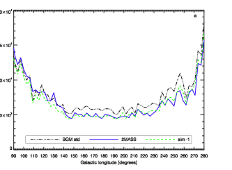
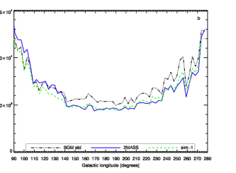
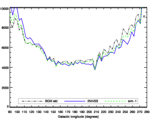
Figure 2: Longitudinal profile for star counts for three ranges of Galactic latitudes. a) $|b|\leq 0.5^{\circ}$; b) $0.5^{\circ}<|b|\leq 3.5^{\circ}$; c) $|b|>3.5^{\circ}$. The data are plotted in solid lines, the standard BGM with dotted-dashed lines, sim-1 in dashed lines (see text). The Orion spiral tangents are located at approximately at $\ell\sim 80$ and 260^∘.

4 The optimisation procedure

In order to fit model parameters, we have used a genetic algorithm, a method based on evolutionary mechanisms and theories, using selections of models similar to natural selection and genetics. This method presents some characteristics which make this technique more efficient than the usual heuristic methods based on calculus, either random or enumerative processes as pointed out by Holand (1975) and Mitchell (1996), and references therein. The GAs are also related to artificial intelligence, having the ability to learn by experimenting, as used in many computational domains.

In astronomy, different versions of the GA have been employed in several different applications, involving Galaxy modelling, such as Sevenster et al. (1999) and stellar population diagnostics by colour-magnitude diagrams (Ng 1998; Ng et al. 2002). In another instance, Larsen & Humphreys (2003) applied the GA to retrieve eight parameters of the Galactic structure. They performed comparisons between their model counts and the data from the Automated Plate Scanner Catalog for 88 fields.

In the present work, we have used the version of GA called PIKAIA. This optimisation subroutine was first presented by Charbonneau (1995) and Charbonneau & Knapp (1996). PIKAIA works with 12 parameters (Charbonneau 1995). The choice for the values of those parameters depends on the application. After some tests, we chose the values of these parameters described in Table 3. Some of them are slightly different from the standard ones; they are appropriate when a large number of parameters are adjusted. They force a higher search in the space of parameters, as for instance, the crossover probability and the maximum mutation rate.

The ngen parameter defines the number of the generations used. In our case, a too-small value would cause a premature solution. On the other hand, we identified that for our problem, there is no significant improvement in the $\chi^{2}$ with ngen values of greater than 300.

Table 3: Values of the parameters set in PIKAIA with their meaning in comparison with the standard ones.

Parameter	Present work	Default	Identifier name
ng	100	100	number of individuals in a population
ngen	300	500	number of generations over which solution is to evolve
nd	5	6	number of significant digits
crossover	0.90	0.85	crossover probability
mut	2	2	mutation mode: 1 - one-point mutation, fixed rate; 2 - one-point, adjustable rate based on fitness;
			3 - one-point, adjustable rate based on distance; 4 - one-point + creep, fixed rate;
			5 - one-point+creep, adjustable rate based on fitness;
			6 - one-point+creep, adjustable rate based on distance
imut	0.005	0.005	initial mutation rate
pmutmn	0.0005	0.0005	minimum mutation rate
pmutmx	0.35	0.25	maximum mutation rate
fdif	1.0	1.0	relative fitness differential
irep	1	3	reproduction plan: 1 - full generational; 2- steady state replace-random;
			3 - state-replace-worst (only with no elitism)
ielite	1	0	elitism: 1=on, 0=off

The nd parameter defines the number of significant digits retained in chromosomal encoding (Charbonneau 1995). For the parameters used in the present work, a value of 5 for $nd$ was found to be the most reasonable value as a compromise between accuracy and performance. Indeed a run with nd = 6 gave similar parameter values and $\chi^{2}$. Regarding CPU time, the difference was approximately 10% larger than with nd = 5.

We also have used the elitism technique that consists of storing away the parameters of the best-fit member of the current population and later copying them into the offspring population (Charbonneau 1995). Use of this technique also avoids a lost solution of good gens by either mutation or crossover. As we have used elitism, it is necessary to use the options (irep) 1 or 2 (see Table 3) in the reproduction plan. We have used the option irep = 1 (full generational replacement). We also did a run using irep = 2, but the $\chi^{2}$ was similar, as well as the parameters, considering the range of standard deviation.

The main procedure consisted of comparing the counts obtained from drawn parameters with the observed data, and making the parameters evolve to improve the figure of merit. In order to optimise the process and to avoid recomputing all simulations each time the model parameters are changed, we attribute to each star ($s$) of coordinates (x,y,z) a weight ($w_{\mathrm{s}}$) which is the ratio between the new density ($\rho_{\mathrm{new}}(x,y,z)$) obtained by parameter fitting and the standard one ($\rho_{\mathrm{std}}(x,y,z)$) obtained with BGM standard parameters, as described below:

$$w_{\mathrm{s}}=\frac{\rho_{\mathrm{new}}(x,y,z)}{\rho_{\mathrm{std}}(x,y,z)},$$ (6)

This was only applied to the thin disc population. Other populations were unchanged in the process. Positions are given as a function of Galactocentric cartesian coordinates (x,y,z).

The total number of stars (N_i,new) modelled (for the given set of parameters) for each bin (i) is given by Eqn 7:

$$N_{i,\rm new}=\sum_{s=1}^{N_{i,\rm std}}w_{\mathrm{s}}.$$ (7)

N_i,std is the number of stars in the bin (i) in the standard model.

The merit function is presented in Eqn 8:

$$\chi^{2}=\sum_{i=1}^{N_{\rm bin}}(N_{i,\rm obs}-N_{i,\rm new})^{2}/(N_{i,\rm obs}+N_{i,\rm new})^{2},$$ (8)

$N_{i,\rm obs}$ is the number of stars in bin (i) observed by 2MASS, N_bin is the number of bins (1615) and N_i,new defined in Eqn 7.

We preferred to use this relation instead of traditional $\chi^{2}$ in order to have a reasonable weight for bins with a large number of stars. We note that a relative $\chi^{2}$ avoids overweighting the contribution of latitude bins with high star counts but without necessarily high contrast. Larsen & Humphreys (2003) used a similar one. As a reference, the total $\chi^{2}$ of the standard model is 33.32 for 1615 bins, distributed in 14.70 towards second quadrant (784 bins) and 18.62 towards third quadrant (831 bins). Table 4 shows the range of parameters involved in those simulations.

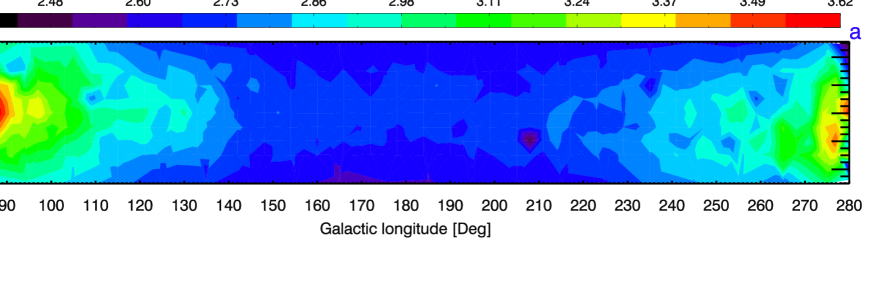
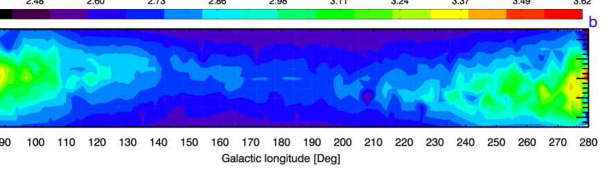
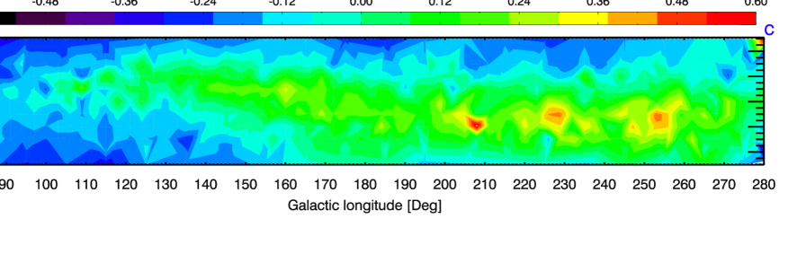
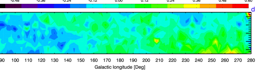
Figure 3: Maps of star counts per square degree and residuals of the fit for standard model and sim-1: a) observed 2MASS star counts; b) standard model star counts; c) relative residuals for standard model; d) relative residuals for sim-1 (Eqn 5). The values are binned ($\Delta\ell=3^{\circ}$ and $\Delta b=0.5^{\circ}$) and interpolated. The Orion spiral tangents are located at approximately at $\ell\sim$ 80 and 260^∘.

Table 4: The range of the parameter values used in sim-1.

Component	Parameter	Unit	Range
warp	$\gamma_{\mathrm{warp_{+}}}$	pc kpc-1	[0.01;0.81]
	$\gamma_{\mathrm{warp_{-}}}$	pc kpc-1	[0.01;0.81]
	$R_{\mathrm{warp}}$	pc	[7000;12000]
	$\theta_{\mathrm{warp}}$	rad	[0;$2\pi$]
flare	$\gamma_{\mathrm{flare}}$	kpc-1	[0.005;0.055]
	$R_{\mathrm{flare}}$	pc	[8000;11000]
scale length	kp1	pc	[3500;6500]
	kp2…7	pc	[1200;3700]
disc truncation	Rdis	pc	[12000;22000]
	hcut	pc	[500;1500]

5 Results

5.1 Fitting the parameters of the standard model

The standard BGM works with two scale lengths for disc stars, first one, kp₁, for stars with age $<$ 0.15 Gyr and the second one, kp_2…7, for stars ranging from 0.15 to 10.0 Gyr (see also Table 1). We performed a set of fitting procedures (sim-1) with 100 independent runs of 300 generations each, considering these two scale lengths for disc stars, and warp and flare parameters. Table 5 summarises the fitted parameters in sim-1, as well as the median and standard deviation for each parameter.

Table 5: Parameters obtained for sim-1: median and standard deviation for 100 independent runs. A unique scale length is considered for age class 2 to 7, noted by kp_2…7. $Lr$ is the reduced likelihood and BIC is the Bayesian information criterion, see Eqn 16 and text in Section 5.2.

Parameter	Unit	sim-1
$\gamma_{\mathrm{warp_{+}}}$	pc kpc-1	0.626 $\pm$ 0.047
$\gamma_{\mathrm{warp_{-}}}$	pc kpc-1	0.165 $\pm$ 0.021
$R_{\mathrm{warp}}$	pc	9108 $\pm$ 144
$\theta_{\mathrm{warp}}$	rad	3.292 $\pm$ 0.024
$\gamma_{\mathrm{flare}}$	kpc-1	0.23 $\pm$ 0.04
$R_{\mathrm{flare}}$	pc	8923 $\pm$ 191
kp1	pc	3852 $\pm$ 167
kp2…7	pc	2477 $\pm$ 48
Rdis	pc	16081 $\pm$ 1308
hcut	pc	717 $\pm$ 272
$\chi^{2}$	———-	21.80 $\pm$ 0.08
$Lr$	———-	-20029.8
BIC	———-	40133.4

The scale length for stars with age larger than 0.15 Gyr is best fitted by a scale length of 2.48 kpc. This value is similar to the scale length used in the standard BGM, and also in agreement with many recent studies (see discussion in Section 6). As shown in Table 5, the warp is found asymmetrical, with a stronger slope in the third quadrant than in the second quadrant. The flare is also very significant. The starting radius of the flare is close to the starting radius of the warp.

Figure 2 shows longitudinal profiles for sim-1 versus BGM standard and 2MASS data for three ranges of Galactic latitudes. There is a net improvement with the new fits at nearly all longitudes.

Depending on latitudes, the sim-1 model performs better or similarly to the standard BGM. For example, the agreement is better at $|\emph{b}|<$ $0.5^{\circ}$, apart from the longitude $\ell<100^{\circ}$ where it is similar. Though, at the same longitudes but higher latitudes (b $>$ 3.5^∘) sim-1 is much better. Overall, sim-1 performs much better than the standard model, although it is not perfect everywhere. We expect that a more complex model might give a better solution (see Section 5.2).

Indeed, part of the differences at $\ell\sim 80^{\circ}$ could be attributed to the Local Arm (Drimmel 2000) that is not modelled in the present work. He also pointed out that the counterpart of the Local arm is centred at $\ell\sim 260^{\circ}$, where we also see some disagreement between our model and 2MASS data. The fitting of spiral arms using BGM with 2MASS data is outside of the scope of the present paper. It will be analysed in detail in a forthcoming paper where we attend to fit a spiral model including data from the inner Galaxy.

The irregular profile can be due to the interval of bins in longitude and because each field has its extinction, photometric errors and completeness limits. Another source of error resides on the fact that the map of Marshall (2009) has a lower resolution for outer Galaxy fields than for inner part. For instance in some fields, we got extinction determination for a distance of approximately 0.5 degrees of the centre of our field.

Figures 3a and 3b show the counts observed by 2MASS and modelled by BGM Standard, respectively. Figures 3c and Figures 3d show the ($\ell$,b) map of the relative residuals for the standard model and sim-1, respectively. In Fig. 3c, some regions in orange, red, yellow show where the standard model predicts more counts than observed. An interesting pattern is that the position of the mid-plane slightly differs in the model from the data. This is particularly the case in the second quadrant between $\ell\sim$ 120^∘ and 180^∘. In the third quadrant, the mid-plane seems to be almost correctly placed but, the model overestimates the counts at latitudes $\sim 0^{\circ}$. A similar feature, due to dissymmetry of the disc in the warp and probably in disc truncation, has been pointed out by Reylé et al. (2009). They show that the warp slope was different in the second and third quadrants. While the differences towards $\ell\sim 90^{\circ}$ and 270^∘ can be attributed mainly to the warp, the overdensities found in Galactic anti-centre are probably due to the disc scale length, disc edge and flare effects, as it is investigated below.

In Fig. 3d, in the comparison of sim-1 with 2MASS data, we can identify that most of the fields for both second and third quadrants have a relative difference in the range of 0$-20\%$. A minuscule area can be seen at ($\ell$,b) $\sim$ (210^∘, -2^∘). We note that in analysing the Marshall (2009) extinction map, this region has a high extinction with A_V of about 10 to 12 mag, while in the neighbouring fields the extinction drops to four magnitudes in A_V. This explains the reduced counts not only in the model counts but also in 2MASS data as can be seen in Fig. 3a. This high extinction area is not well taken into account in the 3D extinction model used.

Figure 4: Histogram of the differences. Upper: Absolute difference, $N_{i,\rm model}-N_{i,\rm obs}$ per bin; Lower: relative difference. Standard model (solid line), sim-1 (dotted-dashed line).

It can also be seen that both second and third quadrants present a significant improvement with regards to the standard model. We note that it is still better in the third quadrant, apart from the region of the local arm. Some residuals appear larger than 10% at $\ell\sim$ 140^∘, which could be related to the outer arm, not included here. After the optimisation procedure, most of the fields with green colour, for example, relative differences around 30-40%, decreases to residuals smaller than 20%. Figure 4 (upper panel) shows the histogram of the differences $N_{i,\rm model}-N_{i,\rm obs}$ per bin for the standard model and sim-1. As can be seen in Figure 4 (lower panel), there is a significant increase of bins with a relative difference of less than 20% in sim-1.

Figure 5: Colour-magnitude diagrams ($K_{\rm s}$, $J-K_{\rm s}$) for eight directions with their coordinates (in degrees) presented at the top of each panel: red diamonds representing 2MASS data and blue diamonds representing BGM Standard.

In order to investigate whether the discrepancies between simulations and data can be attributed to the interstellar extinction, we have analysed eight colour-magnitude diagrams ($K_{\rm s}$, $J-K_{\rm s}$) towards the regions with substantial differences in the modelled counts. Figure 5 shows those diagrams for 2MASS data and simulations with the standard model. It is clear that the extinction cannot be invoked to interpret the difference in star counts seen between 2MASS data and the model, the colours being in good agreement. We note that both standard BGM simulations and the fitted models named sim-1 and sim-2 (see next section) use the same extinction map.

To improve the model, we have explored whether dependencies of parameters with age can better describe the observed data. This is presented in the next section.

Table 6: Parameters obtained for sim-2 and sim-3 with parameters dependent on age (expressions shown in Eqn 9 to 15). For sim-3, we have considered the ripples (see Section 5.5). The likelihood $Lr$ and the Bayesian Information Criterion BIC are explained in Eqn 16 and in Section 5.2

.

Parameter	Range	sim-2	sim-3
$a_{\gamma_{\mathrm{warp_{+}}}}$ (pc kpc-1)	[0.0;1.30]	1.033 $\pm$ 0.221	0.993 $\pm$ 0.237
$b_{\gamma_{\mathrm{warp_{+}}}}$ (pc kpc-1 Gyr${}^{-1})$	[0.15;0.75]	0.357 $\pm$ 0.139	0.367 $\pm$ 0.133
$c_{\gamma_{\mathrm{warp_{+}}}}$ (pc kpc-1 Gyr${}^{-2})$	[0.02;0.12]	0.053 $\pm$ 0.024	0.056 $\pm$ 0.024
$a_{\gamma_{\mathrm{warp_{-}}}}$ (pc kpc-1)	[0.05;0.40]	0.062 $\pm$ 0.031	0.074 $\pm$ 0.039
$b_{\gamma_{\mathrm{warp_{-}}}}$ (pc kpc-1 Gyr${}^{-1})$	[0.06;0.26]	0.082 $\pm$ 0.019	0.083 $\pm$ 0.019
$a_{R_{\mathrm{warp}}}$ (kpc)	[7000;12000]	10189 $\pm$ 395	10510 $\pm$ 446
$b_{R_{\mathrm{warp}}}$ (kpc Gyr${}^{-1})$	[100;600]	255 $\pm$ 74	301 $\pm$ 80
$a_{\theta_{\mathrm{warp}}}$ (rad)	[2.50;3.50]	3.382 $\pm$ 0.056	3.376 $\pm$ 0.058
$b_{\theta_{\mathrm{warp}}}$ (rad Gyr${}^{-1})$	[0.03;0.23]	0.058 $\pm$ 0.012	0.055 $\pm$ 0.011
$a_{R_{\mathrm{flare}}}$ (kpc)	[7000;11000]	8024 $\pm$ 316	7992 $\pm$ 324
$b_{R_{\mathrm{flare}}}$ (kpc Gyr${}^{-1})$	[300;1300]	922 $\pm$ 193	929 $\pm$ 239
$a_{\gamma_{\mathrm{flare}}}$ (kpc${}^{-1})$	[0.15;0.65]	0.359 $\pm$ 0.121	0.328 $\pm$ 0.117
$b_{\gamma_{\mathrm{flare}}}$ (kpc-1 Gyr-1)	[0.01;0.16]	0.051 $\pm$ 0.039	0.0601$\pm$ 0.035
Rdis (pc)	[12000;22000]	19482 $\pm$ 1419	18742 $\pm$ 1601
hcut (pc)	[500;1500]	955 $\pm$ 316	1070 $\pm$ 274
$h_{\rm ra}$ (pc)	[1500,3000]	2357 $\pm$ 148	2436 $\pm$ 125
$h_{\rm rb}$ (pc Gyr-1)	[700;2700]	742 $\pm$ 114	743 $\pm$ 80
$h_{\rm rc}$ (pc Gyr-2)	[0.20;0,80]	0.397$\pm$ 0.210	0.513$\pm$ 0.191
kp1 (pc)	[3500;6500]	3771 $\pm$ 292	3798$\pm$ 277
$\chi^{2}$	—————	20.16 $\pm$ 0.12	20.24 $\pm$ 0.14
$Lr$	—————	-17957.4	-18020.0
BIC	—————	36055.1	36180.3

Table 7: Correlations for sim-1.

	$\gamma_{warp_{+}}$	$\gamma_{warp_{-}}$	$R_{\mathrm{warp}}$	$\gamma_{\mathrm{flare}}$	$R_{\mathrm{flare}}$	kp2…7	$R_{\mathrm{dis}}$	$h_{\mathrm{cut}}$
$\gamma_{\mathrm{warp_{+}}}$	1.000	0.298	0.525	0.032	0.160	-0.198	0.172	-0.192
$\gamma_{\mathrm{warp_{-}}}$	0.298	1.000	0.800	0.042	0.100	-0.287	0.080	-0.321
Rwarp	0.525	0.800	1.000	-0.334	-0.160	-0.310	0.246	-0.485
$\gamma_{\mathrm{flare}}$	0.032	0.042	-0.334	1.000	0.813	0.178	-0.065	0.618
Rflare	0.160	0.100	-0.160	0.813	1.000	-0.126	0.063	0.339
kp2…7	-0.198	-0.287	-0.310	0.178	-0.126	1.000	-0.164	0.467
Rdis	0.172	0.080	0.246	-0.065	0.063	-0.164	1.000	-0.066
hcut	-0.192	-0.321	-0.485	0.618	0.339	0.467	-0.066	1.000

5.2 Dependence of the warp, flare and scale length with age

In order to investigate whether the warp and flare parameters depend on age (as the scale length), and to constrain the warp formation scenario, four sets of simulations were performed dividing the ages into two groups, as the number of parameters to fit would be too high to estimate the warp shape individually for each Age Class bin. For instance, the first run of optimisation considered one group for the stars with AC $=1$ and another group for stars with AC $\geq 2$; the second run, one group for stars with AC $\leq 2$, and the other group for stars with AC $\geq 3$, and so on. Those tests showed that the dependence on age can be modelled linearly for most of the parameters, except for the warp in the second quadrant, which follows roughly a second order polynomial.

Then, we performed new fits assuming age dependencies of parameters, either linearly or as a second order polynomial, as given in Eqs 9 to 15 below with the units provided in Table 6.

Table 8: Correlations for sim-2.

	a${}_{\gamma_{\mathrm{warp_{+}}}}$	b${}_{\gamma_{\mathrm{warp_{+}}}}$	c${}_{\gamma_{\mathrm{warp_{+}}}}$	a${}_{\gamma_{\mathrm{warp_{-}}}}$	b${}_{\gamma_{\mathrm{warp_{-}}}}$	a${}_{R_{warp}}$	b${}_{R_{warp}}$	a${}_{\theta_{warp}}$	b${}_{\theta_{warp}}$	a${}_{R_{flare}}$	b${}_{R_{flare}}$	a${}_{\gamma_{flare}}$	b${}_{\gamma_{flare}}$	Rdis	hcut	$h_{\rm ra}$	$h_{\rm rb}$	$h_{\rm rc}$	kp1
a${}_{\gamma_{\mathrm{warp_{+}}}}$	1.000	0.769	0.478	0.109	0.014	0.110	0.067	0.088	0.082	-0.104	0.339	0.056	0.151	-0.114	-0.143	-0.081	-0.087	-0.128	0.157
b${}_{\gamma_{\mathrm{warp_{+}}}}$	0.769	1.000	0.915	-0.128	0.027	-0.247	-0.344	-0.147	-0.207	0.080	0.401	0.209	0.084	0.008	-0.169	-0.083	0.021	-0.177	-0.151
c${}_{\gamma_{\mathrm{warp_{+}}}}$	0.478	0.915	1.000	-0.224	0.090	-0.287	-0.441	-0.165	-0.289	0.151	0.369	0.219	0.058	0.044	-0.162	-0.020	0.038	-0.149	-0.323
a${}_{\gamma_{\mathrm{warp_{-}}}}$	0.109	-0.128	-0.224	1.000	-0.298	0.376	0.407	-0.114	-0.037	-0.008	-0.188	-0.092	0.079	-0.149	0.176	0.095	-0.124	0.012	0.030
b${}_{\gamma_{\mathrm{warp_{-}}}}$	0.014	0.027	0.090	-0.298	1.000	0.096	-0.113	0.173	0.566	-0.061	0.423	0.151	-0.035	-0.025	-0.004	0.446	-0.300	0.220	-0.097
a${}_{R_{warp}}$	0.110	-0.247	-0.287	0.376	0.096	1.000	0.900	0.103	0.037	-0.198	-0.066	-0.328	0.166	-0.165	0.019	0.154	-0.285	0.083	0.105
b${}_{R_{warp}}$	0.067	-0.344	-0.441	0.407	-0.113	0.900	1.000	0.021	-0.054	-0.096	-0.204	-0.252	0.219	-0.118	0.119	0.127	-0.256	0.008	0.195
a${}_{\theta_{warp}}$	0.088	-0.147	-0.165	-0.114	0.173	0.103	0.021	1.000	0.772	-0.201	0.240	-0.023	0.027	-0.150	-0.139	0.266	-0.124	0.369	0.079
b${}_{\theta_{warp}}$	0.082	-0.207	-0.289	-0.037	0.566	0.037	-0.054	0.772	1.000	-0.220	0.384	0.077	-0.063	-0.083	-0.010	0.380	-0.231	0.403	0.183
a${}_{R_{flare}}$	-0.104	0.080	0.151	-0.008	-0.061	-0.198	-0.096	-0.201	-0.220	1.000	-0.387	0.710	-0.463	0.046	0.304	0.131	-0.091	-0.103	-0.578
b${}_{R_{flare}}$	0.339	0.401	0.369	-0.188	0.423	-0.066	-0.204	0.240	0.384	-0.387	1.000	0.190	0.350	0.041	-0.211	0.193	-0.006	0.212	0.004
a${}_{\gamma_{flare}}$	0.056	0.209	0.219	-0.092	0.151	-0.328	-0.252	-0.023	0.077	0.710	0.190	1.000	-0.428	0.163	0.266	0.275	0.055	0.113	-0.392
b${}_{\gamma_{flare}}$	0.151	0.084	0.058	0.079	-0.035	0.166	0.219	0.027	-0.063	-0.463	0.350	-0.428	1.000	-0.215	-0.066	0.058	-0.048	-0.081	0.092
Rdis	-0.114	0.008	0.044	-0.149	-0.025	-0.165	-0.118	-0.150	-0.083	0.046	0.041	0.163	-0.215	1.000	-0.154	0.095	0.129	0.265	0.051
hcut	-0.143	-0.169	-0.162	0.176	-0.004	0.019	0.119	-0.139	-0.010	0.304	-0.211	0.266	-0.066	-0.154	1.000	0.095	-0.009	-0.029	-0.032
hra	-0.081	-0.083	-0.020	0.095	0.446	0.154	0.127	0.266	0.380	0.131	0.193	0.275	0.058	0.095	0.095	1.000	-0.562	0.758	-0.219
hrb	-0.087	0.021	0.038	-0.124	-0.300	-0.285	-0.256	-0.124	-0.231	-0.091	-0.006	0.055	-0.048	0.129	-0.009	-0.562	1.000	-0.172	0.076
hrc	-0.128	-0.177	-0.149	0.012	0.220	0.083	0.008	0.369	0.403	-0.103	0.212	0.113	-0.081	0.265	-0.029	0.758	-0.172	1.000	-0.062
kp1	0.157	-0.151	-0.323	0.030	-0.097	0.105	0.195	0.079	0.183	-0.578	0.004	-0.392	0.092	0.051	-0.032	-0.219	0.076	-0.062	1.000

$$\gamma_{\mathrm{warp_{+}}}=a_{\gamma_{\mathrm{warp_{+}}}}-b_{\gamma_{\mathrm{warp_{+}}}}\times<\rm age_{i}>+c_{\gamma_{\mathrm{warp_{+}}}}\times<\rm age_{i}>^{2},$$ (9)

$$\gamma_{\mathrm{warp_{-}}}=a_{\gamma_{\mathrm{warp_{-}}}}+b_{\gamma_{\mathrm{warp_{-}}}}\times<\rm age_{i}>,$$ (10)

$$R_{\mathrm{warp}}=a_{R_{\mathrm{warp}}}-b_{R_{\mathrm{warp}}}\times<\rm age_{i}>,$$ (11)

$$\theta_{\mathrm{warp}}=a_{\theta_{\mathrm{warp}}}-b_{\theta_{\mathrm{warp}}}\times<\rm age_{i}>,$$ (12)

$$R_{\mathrm{flare}}=a_{R_{\mathrm{flare}}}+b_{R_{\mathrm{flare}}}\times<\rm age_{i}>,$$ (13)

$$\gamma_{\mathrm{flare}}=a_{\gamma_{\mathrm{flare}}}+b_{\mathrm{flare}}\times<\rm age_{i}>,$$ (14)

The scale length also has a tendency to decrease with age in those simulations. Hence, we adopted a dependence as shown in Eq. 15, which adequately follows the variations seen in the tests with two age groups.

$$h_{\rm R}=h_{\rm ra}+h_{\rm rb}\times{\rm exp}(-h_{\rm rc}<\rm age_{i}>),$$ (15)

where $<\rm age_{i}>$ is the mean age of Age Class $i$, as indicated in Table 1.

Using the equations above, with the range of parameters given in Table 6 (second column), we have performed a new set of optimisations (called sim-2) with 100 independent runs, using the ranges of parameters presented in Table 6, together with the best fit values and estimated uncertainties. Eqn 15 is applied on ages from 0.15 to 10 Gyr, while the first age bin is fitted with the parameter kp₁, as in sim-1. The standard errors can be high in some cases, such as $c_{\gamma_{\mathrm{warp_{+}}}}$ and $b_{\gamma_{\mathrm{flare}}}$. Although their impact on our estimates of the warp and flare shapes is limited and concerns mainly oldest stars, as will be shown in Figs. 7 and 8.

As can be seen in the comparison of $\chi^{2}$ in tables 5 and 6, there is an improvement of $\chi^{2}$ in sim-2 compared to sim-1. To estimate the number of parameters and the effective improvement in the $\chi^{2}$, we compute the Bayesian information criterion (BIC) (Schwarz et al. 1978). We follow the recipes of Robin et al. (2014) first computing the reduced likelihood ($Lr$, Eqn 16) for a binomial statistics (Bienaymé et al. 1987), as described below:

$$Lr=\sum_{i=1}^{n}q_{i}\times(1-R_{i}+\mathrm{ln}(R_{i})),$$ (16)

where $f_{i}$ and $q_{i}$ are the number of stars in bin $i$ in the model and the data, and $R_{i}=\frac{f_{i}}{q_{i}}$.

The BIC is then computed following the formula from Schwarz et al. (1978), $BIC=-2\times Lr+k\times\mathrm{ln}(n)$. It penalises models with a larger number of parameters and allows to compare the goodness of fit of different models with a different number of fitted parameters. $n$ is the number of bins on which the data are fitted and k the number of fitted parameters. In our case, $n$ = 1615, and k = 10 and 19 for sim-1 and sim-2, respectively.

Then, $Lr$ (Eqn 16) and the BIC were computed for the three fitting procedures with their values showed in Table 5 (sim-1) and Table 6 (sim-2 and sim-3). The BIC for sim-2 and sim-3 are quite similar despite the fact that sim-3 incorporates extra parameters to model the ripples, but we did not adjust these parameters. Hence the number of fitted parameters k is the same in sim-2 and sim-3. The comparison between sim-1 and sim-2 highlights the fact that sim-2, despite using more parameters than sim-1, is preferred on the criterion of goodness of fit.

The values obtained for each parameter in sim-2 are given in Table 6 (third column). The map of the relative differences between sim-1 and sim-2 (N_sim-2-N_sim-1)/N_sim-1 is presented in Figure 6. The average difference is around 10%. There are two main large area where the two fitted models differ. The first one at $\ell\sim 150^{\circ}$ and b $<-2^{\circ}$ where sim-2 produces more counts than sim-1, and the area around $\ell\sim 200^{\circ}$ where it produces less. The shape of the residuals seems to indicate that the change in the mean scale length with age in sim-2 affects the counts in the anti-centre, as expected. But also the shape of the warp varying with time has an impact on the star counts at the level of about 10 to 15% in the specific area at $\ell\sim 150^{\circ}$ and b $<-2^{\circ}$.

Figure 6: Map of the relative differences between sim-2 and sim-1 (N_sim-2-N_sim-1)/N_sim-1.

Figure 7: Dependence of warp parameters: amplitude in the second quadrant (top left) and in the third quadrant (top right); starting radius (bottom left) and angle (bottom right) obtained in sim-2 using Eqn 9 to 12 with parameters provided in Table 6. Circles represents outliers (see text). In the top left panel, the whiskers are not shown at 8.5 Gyr because they are too large (0.371 and 3.639).

The variation of the warp, flare and scale length with age over the 100 different independent solutions are presented in Figs 7 to 9, respectively. The box plots were produced by using IDL Coyote’s Library; the box encloses the InterQuartile Range (IQR), defined as Q₃ - Q₁, in which Q₃ and Q₁ are the upper and lower quartile, respectively. The whiskers extend out to the maximum or minimum value of 100 independent solutions, or to the 1.5 times either the Q₃ or Q₁, if there is data beyond this range. The small circles are outliers, defined as values either greater or lower than 1.5 $\times$ Q₃ or Q₁.

We note that all warp parameters significantly change with age (Figure 7). The slope of the warp for both second and third quadrants varies as a function of age. The shapes significantly vary from second to third quadrant, even though error bars are larger in the third quadrant and for stars older than 6 Gyr. One common aspect resides on the fact that the amplitude increases for stars with age greater than 4 Gyr for both quadrants.

These figures show that the warp shape changes significantly with time (or with the age of the tracers), and the variations are different in the second and in the third quadrants. The starting radius of the warp changes monotonically with age, as well as the node angle. But for young stars, the slope of the warp is very different between second and third quadrants. This confirms the strong dissymmetry between the region of the plane moved to positive latitudes (first and second quadrants) and the opposite region (third and fourth quadrant), but points out that this dissymmetry is mainly due to young stars, while old stars follow a more symmetrical warp, even though the error bars for old stars are larger.

Figure 8: Dependence with age of the flare parameters, as given in Table 6 and Eqn 13 and 14: amplitude (upper panel) and starting radius (lower panel).

The asymmetry of the warp was long identified in HI gas (Burton 1988; Levine et al. 2006; Kalberla & Dedes 2008) and even in stars (López-Corredoira et al. 2002; Reylé et al. 2009). But this is the first time that it is shown that the shape varies with the age of the tracers considered.

The flare also exhibits a time dependence (Figure 8). Despite the fact that error bars of the flare amplitude increase with time, there is a clear trend showing that the amplitude increases with age. The starting radius of the flare also varies with age. We shall consider in Section 5.4 whether these features can be due to correlations.

Figure 9 shows the scale length variation with age obtained with sim-2 using Equation (15). The values of the fitted parameters are given in Table 6. As can be seen in this figure, the scale length clearly decreases with age. This result, which is related to the thin disc formation scenario, will be discussed in Section 6.

5.3 Disc truncation

As seen in Table 5 with sim-1, the disc truncation (R_dis) is found at approximately 16.1 $\pm$ 1.3 kpc. The scale (h_cut) of cutoff is equal to 0.72 $\pm$ 0.27 kpc. It is such that the density drops by 90% within 1 kpc, therefore, the cutoff is sharp. In sim-2, when age dependence for warp, flare and scale length is considered the disc truncation obtained is 19.4 $\pm$ 1.4 kpc and considering the ripples (sim-3, see Section 5.5) is 18.7 $\pm$ 1.6 kpc, still in agreement at the $1-\sigma$ level with its value in sim-1.

We note that the disc truncation is found at a larger Galactocentric distance than in the standard model, where it was assumed 14 kpc. The determination is here more robust than in Robin et al. (1992a) from which the standard model was based, since only one direction was used for that determination.

5.4 Parameter correlations

In order to investigate whether the parameters are correlated, we computed the correlation coefficients in the optimisation procedure sim-1, shown in Table 7, and in Figure 12 in the Appendix. R_flare and $\gamma_{\mathrm{flare}}$ are fairly correlated because we have considered only low latitude fields in our study. The same problem was mentioned by López-Corredoira et al. (2002) and López-Corredoira & Molgó (2014). A significant correlation also appears between R_warp and the warp amplitude specially in the third quadrant.

Table 8 shows the correlations among the parameters for sim-2. As can be seen, some parameters are correlated (notably the starting radius and the amplitudes of the warp and flare). This is expected because the photometric distances are not precise enough. Hence, the exact position where the flare starts is not well determined, and it probably starts more smoothly than a linear increase starting at a given point. But the overall measurements of the warp and flare dependencies with age are clear enough and not impacted by those correlations. To avoid these correlations, in the future several complementary studies should be considered. Firstly, looking at higher latitudes, covering latitudes from -30^∘ to +30^∘ in the anti-centre direction would allow disentangling the effect of the flare from the radial truncation. Secondly, the correlation between the starting radius and the amplitude is due to a simplistic linear shape used. Using samples with good distance estimates, such as Gaia data or red clump giants, would allow to determine better the shape of the starting radius and the amplitude of the flare.

5.5 Is there an improvement considering the ripples ?

We also considered in another set of simulations (sim-3), the contribution of ripples, an oscillation in the number of star counts, as described by Xu et al. (2015) without fitting any parameter of the ripple itself. They have used SDSS data towards 110^∘ $<$ $\ell$ $\leq$ 229^∘ in order to study the structures in the outer Galaxy. We have used the same equations for the northern and southern, as provided by Xu et al. (2015) in Section 6 of their paper.

Basically, when computing z_w we add the z_wripple given by Xu et al. (2015). The resulting parameters and the $\chi^{2}$ of the solution are given in Table 6, showing no improvements compared with sim-2 but rather a slightly higher BIC value.

6 Discussion

6.1 Thin disc scale length

The disc scale length is the most important unknown in disentangling the contributions from the disc and the dark halo to the mass distribution of the Galaxy (Dehnen & Binney 1998; Bovy & Rix 2013). Recently, the thin disc scale length has been studied from photometric and spectroscopic large scale surveys. For example, Bovy et al. (2012) determine various scale lengths for mono-abundance populations. Assuming that the thin disc is defined by the low $\alpha$ abundance population, they show that the scale length can depend on the metallicity within the thin disc. In their sample high metallicity stars have a shorter scale length than low metallicity ones, with noticeably large error bars, which is in contradiction with our work if metallicity is anti-correlated with age. However the mean orbital Galactic radii of the low metallicity stars are much larger, which implies that their sample of low metallicity stars comes from the outer Milky Way, while the high metallicity sample comes from the inner Milky Way. In the end, the sample from the outer Milky Way has larger scale length, as expected from the inside-out scenario. The scale lengths of the mono-abundance populations of the thin disc range from 2.4 to 4.4 kpc, while we found a very similar scale length range of 2.3 to 3.9 kpc.

Our result of a short scale length for the main thin disc (as stars older than 3 Gyr dominates the counts in the Milky Way) is in general agreement with previous results. Table 9 shows most of the scale length determinations from different authors during the last twenty years as well as the tracer used and field coverage. It is noticeable that most studies using IR data found a short scale length for the thin disc, compared with longer scale length obtained from visible data. This is understandable if the IR tracers are in the mean older than the visible tracers (young stars emit mostly in the visible). However, this could also be due to the extinction which perturbs the analysis in the visible.

López-Corredoira et al. (2002) constrained the outer disc (scale length, warp and flare) from a study of 2MASS data in 12 fields but only four different longitudes (155^∘, 165^∘, 180^∘ and 220^∘), which does not include fields where the warp is stronger (around 90^∘ and 270^∘). They only use a selection of red giant stars from CMDs and they apply a simple modelling approach assuming a luminosity function and density law for the disc. They find a thin disc scale length of 1.91${}^{0.20}_{-0.16}$ kpc, which is in excellent agreement with our determination for stars older than 3 Gyr, but smaller than our mean scale length. Their sample is dominated by red giants. Hence it does not include higher mass and younger stars, which might explain the difference.

Yusifov (2004) studied the distribution of pulsars from the Manchester et al. (2005) catalogue. Although Momany et al. (2006) claims that the catalogue is incomplete in the outer Galaxy, their scale length for these young objects is 3.8 $\pm$ 0.4 kpc, in close agreement with our young star sample.

As pointed above, Kalberla & Dedes (2008) by fitting HI distribution obtained a radial exponential scale length of 3.75 kpc in the mid-plane. Even if they do not give an estimate of their error, it is in excellent agreement with our very young star scale length of 3.90 $\pm$ 0.28 kpc.

For the first time, we report a clear evolution of the scale length with time among field stars. There have been previous evidences of young stellar associations and young open clusters at distances where the old stars seem to be no more present (Robin et al. 1992b). However, it was long known that the HI disc has a longer scale length than the stars in the mean. Hence, it is not too surprising to see that very young stars have a scale length similar to the gas.

6.2 Disc truncation

The disc truncation has been often observed in external galaxies. The existence of this cut-off can be related to a threshold in the star formation efficiency, when the gas density drops under certain value (Kennicutt 1989; van der Kruit 1979).

We found a radius for disc truncation equal to R_dis = 16.1 $\pm$ 1.3 kpc in the case of sim-1. This value increases up to 18 kpc in the case of sim-2 when the scale length is assumed to vary with time. We have not tested a possible dependence of the truncation on age, in order to avoid increasing too much the number of free parameters. We shall consider this point in the future by extending the fit to higher latitudes, in order to decrease the degeneracy between the flare and the truncation.

Habing (1988) from OH/IR stars and Robin et al. (1992a) from UBV photometry found the edge of Galactic disc located at 14-15 kpc and 14 kpc, respectively. Ruphy et al. (1996) using DENIS data similarly found 15 $\pm$ 2 kpc for the disc truncation distance. These values are in good agreement with our determination. Using photometry for IPHAS stars towards 160${}^{\circ}\leq\ell\leq 200^{\circ}$ ($|b|\leq 1.0^{\circ}$), Sale et al. (2010) obtained a truncation radius of 13.0 $\pm$ 1.1 kpc, slightly smaller than ours, but still within the uncertainties. López-Corredoira et al. (2002) did not find a disc truncation at distances closer than 20 kpc, but indicated that they could not distinguish between a truncation or a flare.

Figure 9: Scale length as a function of age (see text and Eqn 15).

Table 9: Scale length determinations from other authors with tracers and field coverage.

Author	Tracer	Coverage	Scale length (kpc)
Robin et al. (1992a, b)	optical star counts	$\ell=189^{\circ}$	2.5 $\pm 0.3$
Ruphy et al. (1996)	DENIS	$\ell=217,239^{\circ}$	2.3 $\pm 0.1$
Porcelet al. (1998)	TMGS (NIR star counts)	30${}^{\circ}<\ell<70^{\circ}$ for $|b|>$ 5∘	2.1 $\pm 0.3$
Freudenreich (1998)	COBE	whole sky	2.2
Ojha (2001)	2MASS	7 fields for $|b|>$ 12∘	2.8 $\pm$ 0.3
Chen et al. (2001)	SDSS	279 deg2 at high-latitude (49∘ $<|b|<$ 64∘	2.25
Siegel et al. (2002)	optical star counts	optical star counts 14.9 deg2 at $|b|>$ 25∘	2-2.5
López-Corredoira et al. (2002)	2MASS	$\ell=180^{\circ},220^{\circ}$ (b$=0^{\circ},3^{\circ},6^{\circ},9^{\circ},12^{\circ}$)	1.97 ${}^{+0.15}_{0.12}$
		and $\ell=155^{\circ},165^{\circ}$ ($b=0^{\circ}$)
Larsen & Humphreys (2003)	APS catalog (optical)	16 deg2 for $|b|>$ 20∘	3.5
Cabrera-Lavers et al. (2005)	2MASS	$|b|>$ 25∘	2.1
Bilir et al. (2006)	SDSS	6 fields (41${}^{\circ}\leq b\leq 52^{\circ}$)	1.9
Karaali et al. (2007)	SDSS	$\ell=60^{\circ},90^{\circ},180^{\circ}$ ($b=45^{\circ}$, 50∘)	1.65-2.52
Cignoni et al. (2008)	optical open clusters	NGC6819, NGC7789, NGC2099	2.24-3.00
Jurić et al. (2008)	SDSS	$|b|>$ 25∘ (6500 deg2)	2.6 $\pm$ 0.5
Yaz & Karaali (2010)	SDSS	22 fields (0${}^{\circ}<\ell\leq 260^{\circ}$) for (44.3${}^{\circ}\leq b\leq 45.7^{\circ}$)	1.-1.68
Chang et al. (2011)	2MASS	$|b|>$ 30∘	3.7 $\pm$ 1.0
McMillan (2011)	kinematic	————	3.00 $\pm$ 0.22
Bovy et al. (2012)	SDSS/SEGUE	28,000 G-type dwarfs ($|b|>$ 45∘)	3.5 $\pm$ 0.2
Robin et al. (2012)	2MASS	$|\ell|\leq 20^{\circ}$ (-10${}^{\circ}\leq b\leq 10^{\circ}$)	2.5
Cheng et al. (2012)	SDSS/SEGUE	50${}^{\circ}<\ell\leq 203^{\circ}$ ($b=-15.0^{\circ}$,-12.0∘, $\pm$ 8∘,10.5∘,14∘,16∘)	3.4${}^{+2.8}_{-0.9}$

6.3 Warp parameters and origin

Several scenarii have been proposed to explain the Galactic warps, the most cited being a dark halo-disc misalignment and possible interactions with nearby galaxies (or flyby galaxies). Perryman et al. (2014) stated that the misalignment of the disc inside the dark halo might produce changes in the warp angle with time. But in this case, all components of the Galaxy should be perturbed independently of their age. The warp angle dependence that we see could be consistent with this scenario if the time dependence reflects a precession. Alternatively, Weinberg & Blitz (2006) produced dynamical simulations of the flyby of the Magellanic Clouds around the Galaxy which could produce a strongly asymmetric warp varying with time.

However, Reshetnikov et al. (2016) analysed the global structure of 13 edge-on spiral galaxies using SDSS data. They pointed out that the warps found in those galaxies are generally slightly asymmetrical. They studied the relation of the strength and asymmetry of the warps with the dark halo mass. They showed that galaxies with massive halos have weaker and more symmetric warps, concluding that these dark halos play an important role in preventing strong and asymmetric warps. In the case of our Galaxy, the M${}_{\rm tot}/M_{*}$ amount to about 10 (Robin et al. 2003) and the warp angle (computed as seen in edge-on galaxies) is less than 1^∘. Typical galaxies in Reshetnikov’s sample with this mass ratio have warp angles less than 10^∘ and an asymmetry of less than 5^∘. Hence, our Galaxy compares well with these edge-on galaxies having a relatively large dynamical to stellar mass ratio and a weak warp, even though it is asymmetrical.

The Galactic warp can be observed in different components, such as dust, gas and stellar. Reylé et al. (2009) using BGM and 2MASS described the warp and flare, comparing their determination with those provided by several authors from different tracers, such as dust, gas and stars. In this work, they considered R_warp = 8.4 kpc, $\gamma_{\mathrm{warp}}=$ 0.09 pc kpc^-1 for a scale length equal to 2.2 kpc, the same value obtained by Derrière & Robin (2001). Their starting radius was a bit shorter than our mean value of 9.18 kpc.

Figure 10: Comparison of the maximum height of the warp as a function of Galactocentric distance obtained in sim-2 for three different mean ages (dashed lines) with other authors (symbols): López-Corredoira et al. (2002) from red giants (LC02: black open squares), Yusifov (2004) from pulsars (Y04: orange diamonds), Burton (1988) from HI gas (B88: orange plus signs), Levine et al. (2006) model fitted on HI (L06: blue open triangles), Drimmel & Spergel (2001) from COBE/DIRBE data (DS01: black asterisks). Positive (resp. negative) values of z_w refer to second (resp. third) quadrant.

They found evidence that the warp is asymmetric but they were not able to find a good S-shape for the warp in the third quadrant. In the present work, we have adjusted distinct values for the slope of the warp at second and third quadrants. We found a value larger than the one obtained by Reylé et al. (2009), with a slope in the second quadrant approximately three times larger than in the third quadrant. Analysing dust extinction distributions, Marshall et al. (2006) also determined that the warp in the second quadrant has a larger amplitude than in the third quadrant, $\gamma_{\mathrm{warp}}=$ 0.14 and 0.11 pc kpc^-1, respectively. They also pointed out that the warp seems to start earlier in the third quadrant. However, the two parameters ($R_{\mathrm{warp}}$ and $\gamma_{\mathrm{warp}}$) are not completely independent when the warp model is assumed linear.

The difference can be well explained by the fact that we have varied other parameters which were not considered by these authors. They also did not consider the dependence with age, and in the present study we considered a larger range of longitudes, latitudes and limiting magnitude to constrain the model.

Drimmel & Spergel (2001) modelled the Galactic structure by using COBE/DIRBE data at near and far-infrared assuming a warp with a quadratic function $z_{\mathrm{warp}}(\emph{R})=27.4(\emph{R}-R_{\mathrm{warp}})^{2}\sin(\phi)$, with R_warp = 7 kpc. López-Corredoira et al. (2002) model the warp with a different shape than ours. The amplitude of their warp is $2.1\times 10^{-19}\times\emph{R}^{5.25}$. It means that the mid-plane is going up to 1.2 kpc at R = 14 kpc, their node angle is found to be -5^∘$\pm$ 5^∘. They are less sensitive to very young stars than we are because they select mainly red giants in their sample.

Yusifov (2004) models the warp that pulsars follow and find a warp node angle of 14.5^∘, at $1-\sigma$ of our angle for youngest stars. Levine et al. (2006) present a very complex warp shape in HI, which extends at much larger distances, difficult to compare with our simple model.

Momany et al. (2006) studied the distribution of RGB stars to model the outer Galaxy and attempt to explain the Canis Major overdensity. They argue for no outer disc truncation, and that the presence of a strong warp and flare at longitudes of about 240^∘ explain well the overdensity. The study of this particular sub-structure as well as the Monoceros ring is postponed to a future paper.

Figure 10 compares the amplitude of the warp from different authors with our result for three age class. A good agreement is obtained with Burton (1988), López-Corredoira et al. (2002) and Yusifov (2004) for stars with mean age equal to 2.5 Gyr in the distance range, 10.5 $<\emph{R}<$ 13.5 kpc. However, the warp slopes were determined using tracers in different Galactocentric distance ranges. For instance, López-Corredoira et al. (2002) and Yusifov (2004) measurements are claimed by their authors to be valid up to 15 and 18 kpc, respectively. There is also a good agreement between Drimmel & Spergel (2001) and our results for mean age equal to 6.0 Gyr for 9.0 $<R<$ 11.5 kpc. In addition, our estimates of the warp for stars with mean age equal to 0.575 Gyr at negative z_w are in good agreement with Levine et al. (2006), at less than $1.5-\sigma$. The agreement is less good at positive values of z_w, as if the warp effect on stars was different from the HI warp.

We conclude that there is a general consistency between our results and previous ones. The difference between our estimates of the warp shape and other authors can be attributed to the different ranges of longitudes and latitudes covered in each study, as well as to the tracers and methods used. But we are first to claim a warp dependence with the age of the tracers, which is a clue for the scenario of warp formation.

6.4 How does the Galaxy flare in the outskirts

It has been long shown that the HI gas is flaring in the outer Galaxy. This is most probably related to the vertical force (Crézé et al. 1998; Holmberg & Flynn 2000; Kerr & Lynden-Bell 1986; Moni Bidin et al. 2012; Siebert et al. 2003; Sánchez-Salcedo et al. 2011), which is dominated in the inner Galaxy by the stellar disc but in the outer galaxy by dark matter. Hence a good characterization of the K_z and the flare in the outer Galaxy would lead to constrains on its dark matter content.

Kalberla & Dedes (2008) studied the HI distribution in the outer Milky Way and showed that the gas is distributed in two populations. The main gas layer goes to R $\sim$ 35 kpc; the second one goes up to 60 kpc with a very shallow scale length of 7.5 kpc. The first and dominant component is flaring and lopsided. They explain the asymmetry by a dark matter wake towards the Magellanic Clouds. This is much shallower than the flare indicated (see below) by López-Corredoira et al. (2002).

Alard (2000) using 2MASS data studied the flare and warp for longitudes located at $\ell\sim 66.0^{\circ}$, $\ell\sim 180.0^{\circ}$ and $\ell\sim 240.0^{\circ}$ for $|b|<50^{\circ}$ founding evidences for an asymmetry associated with the Galactic warp. He also argued that the flaring and warping seen in the stellar disc is very similar to the characteristics observed in HI disc. López-Corredoira et al. (2002) estimated the flare distance scale to be 4.6 $\pm$ 0.5 kpc, which gives an increase of the scale height by a factor of two at a Galactocentric distance of about 11 kpc and a factor of 10 at 18 kpc. Instead of an exponential, we are using a linear increase of the scale height with Galactocentric radius, which gives a factor of two at 12.2 kpc close to López-Corredoira et al. (2002), and a factor of 4 at about 20 kpc, a less extreme value.

Figure 11 (upper panel) shows a comparison of our flare factor (Eqn 2) with the one of the Alard (2000), López-Corredoira et al. (2002), Yusifov (2004), Kalberla et al. (2014), López-Corredoira & Molgó (2014). To compute the flare factor and compare it with our results, we have divided the flare from other authors by h_z(R${}_{\rm Sun})$ when the flare factor was not given. The values of h_z(R${}_{\rm Sun})$ were taken from Eq. 4 of Kalberla et al. (2014), Eq. 3 of López-Corredoira & Molgó (2014), the Eqn quoted in the abstract of López-Corredoira et al. (2002) and Eq. 7 of Yusifov (2004). The values of h_z(R_Sun) used by each author are indicated in the caption of Figure 11.

Concerning the estimations of errors on the flare factor, Yusifov (2004) mentioned an error around 30% on the pulsar distances determination, López-Corredoira et al. (2002) estimated random errors ranging from 5 to 7%, and López-Corredoira & Molgó (2014) estimated the error to be approximately 18%.

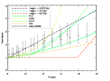
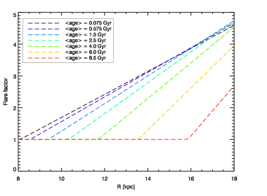
Figure 11: Upper panel: comparison of flare factors (see text for its definition), lines: from López-Corredoira et al. (2002) from red giants (LC02), Yusifov (2004) from pulsars (Y04), Kalberla et al. (2014) from HI gas (K14), López-Corredoira & Molgó (2014) from SDSS-SEGUE data (LC14), and our study (dashed lines). Crosses are the data of Alard (2000) from 2MASS for three range of longitudes: $\ell$ = 66.0^∘, 180^∘ and 240^∘. The values of $h_{\rm z}$(R_Sun) considered for each author were 0.285, 0.580, 0.200, 0.240 and 0.250 pc, respectively. Lower panel: Flare factor for each age class bin in our best fit model from sim-2.

At small distances, all studies give very similar flare factors. In young stars ($<\rm age>\leavevmode\nobreak\ =$ 0.075 Gyr) our flare factor appears similar to López-Corredoira et al. (2002) flare up to 13.0 kpc, and the values are slightly larger for the older stars. For intermediate age stars ($<\rm age>\leavevmode\nobreak\ =$ 2.5 Gyr), a good agreement is seen for a wide range of Galactocentric radius (10.5 kpc $\leq$ R $<$ 16.0 kpc) in comparison with López-Corredoira & Molgó (2014). These authors determine the flare from the SEGUE imaging survey. They fitted a model to F8-G5 stars selected by colours in a sample which did not cover low latitudes $|b|<$ 8^∘, contrarily to our study. They claimed to have found a significant flare but no outer disc truncation. Their flare factor amounts to 3.7 for thin disc stars between the Sun and a Galactocentric distance of 15 kpc, and a factor of 8.3 at a distance of 20 kpc. In comparison, our result points to a factor of 3.8 at 15 kpc and 5.8 at 20 kpc. We assumed a linear slope of the flare to limit the number of parameters. The agreement up to 15 kpc is remarkable. The difference for further distance is most probably due to the disc truncation that we see in-plane.

Yusifov (2004) has a flare scale length of 14 kpc which gives a shallow increase of the scale height with Galactocentric radius, shallower than the HI flare. However, their sample is small (1600 pulsars) and probably incomplete in the outer Galaxy. No estimate of the error bars was given. Hammersley & López-Corredoira (2011) by using five SDSS fields with $|b|>11^{\circ}$ found a smaller amplitude for the flare than obtained, for instance, by Yusifov (2004).

Recently, Feast et al. (2014) identified a few Cepheids at a large distance from the Galactic plane. These Cepheids are a clear example that the young disc is also flaring.

Minchev et al. (2015) attempt to study the effect of the flare on the radial gradient of age, that can be seen in the ”geometrical” thick disc (as defined by the population located at some distance from the Galactic plane, where one expects to be dominated by thick disc stars). They show from numerical simulations that a radial gradient in age naturally emerges due to the flaring of the populations, if younger populations are more extended than older ones. Martig et al. (2016) by using APOGEE data reinforces the results found by Minchev et al. (2015). In our study, the younger disc populations are indeed more extended than older ones, and they also flare earlier. Hence it is expected to produce such age radial gradient at a few kiloparsec distances from the plane. We have not tested this yet, but it will be considered in a future study.

7 Conclusions

We have studied the outer Galaxy structure by using the Besançon Galaxy Model with 2MASS data in order to constrain external disc parameters, such as warp and flare shape, scale length and disc truncation parameters. After the parameter optimisation, the relative difference between the model and 2MASS is generally 10-20% at most, which includes the cosmic variance of the star counts as well as the effect of patchy extinction.

We show strong evidence that the thin disc scale length, as well as the warp and flare shapes, changes with age, and proposed expressions for these dependencies. These results impact directly our comprehension about, not only the shape of those components, but also their origin.

The warp can come from misalignment of the disc inside the dark halo, which might change with time (precession). Alternatively, it can be due to the interaction with the Magellanic Clouds. In both cases, it can imply that tracers of different ages show different spatial distribution, either because there is precession, or because they react differently to the perturbation. The flare could be caused by the fact that the intergalactic gas (or gas coming from Galactic fountains) is falling into the disc more slowly and on longer time scales in the outskirts than in the inner Galaxy. We show in the present work some evidence for their dependence with age that reinforces the point that the warp has a dynamical origin as also demonstrated by López-Corredoira et al. (2007), among others.

Our results clearly show the variation of scale length with the age. The larger scale length for youngest stars (3.9 kpc) is well in agreement with the values found in the HI gas, while the shorter value (2 kpc) for the oldest thin disc is similar to the one of the thick disc. This also directly affects our comprehension of the history of Galactic formation and evolution, reinforcing the idea of an inside-out process of formation.

We also found a disc truncation with R_dis = 16.1 $\pm$ 1.3 kpc. But when we allow the parameters to vary with time, the disc truncation is no more clear and could be at larger distances than 19 kpc, a distance where the stars are scarce anyway, simply due to the exponential fall off. However, this value is not completely independent of other parameters such as the flare and disc scale length.

A further study involving higher latitudes will be considered to strengthen the conclusion about the disc truncation and its dependence with age.

Appendix A Parameters correlations

Figure 12: Correlations between parameters for sim-1 for 100 independent runs.