On the Usability of
Probably Approximately Correct Implication Bases

Abstract

We revisit the notion of probably approximately correct implication bases from the literature and present a first formulation in the language of formal concept analysis, with the goal to investigate whether such bases represent a suitable substitute for exact implication bases in practical use-cases. To this end, we quantitatively examine the behavior of probably approximately correct implication bases on artificial and real-world data sets and compare their precision and recall with respect to their corresponding exact implication bases. Using a small example, we also provide qualitative insight that implications from probably approximately correct bases can still represent meaningful knowledge from a given data set.

1 Introduction

From a practical point of view, computing implication bases of formal contexts is a challenging task. The reason for this is twofold: on the one hand, bases of formal contexts can be of exponential size [14] (see also an earlier work [12] for the same result presented in different terms), and thus just writing out the result can take a long time. On the other hand, even in cases where implication bases can be small, efficient methods to compute them are unknown in general, and running times may thus be much higher than necessary. This is particularly true for computing the canonical basis, where only very few algorithms [9, 15] are known, which all in addition to the canonical basis have to compute the complete concept lattice.

Approaches to tackle this problem are to parallelize existing algorithms [13], or restrict attention to implication bases that are more amenable to algorithmic treatment, such as proper premises [16] or D-bases [1]. The latter usually comes with the downside that the number of implications is larger than necessary. A further, rather pragmatic approach is to consider implications as strong association rules and employ highly optimized association rule miners, but then the number of resulting implications increases even more.

In this work, we want to introduce another approach, which is conceptually different from those previously mentioned: instead of computing exact bases that can be astronomically large and hard to compute, we propose to compute approximately correct bases that capture essential parts of the implication theory of the given data set, and that are easier to obtain. To facilitate algorithmic amenability, it turns out to be a favorable idea to compute bases that are approximately correct with high probability. Those bases are called probably approximately correct bases (PAC bases), and they can be computed in polynomial time.

PAC bases allow to relax the rather strong condition of computing an exact representation of the implicational knowledge of a data set. However, this new freedom comes at the price of the uncertainty that approximation always brings: is the result suitable for my intended application? Of course, the answer to this questions depends deeply on the application in mind and cannot be given in general. On the other hand, some general aspects of the usability of PAC bases can be investigated, and it is the purpose of this work to provide first evidence that such bases can indeed be useful. More precisely, we want to show that despite the probabilistic nature of these bases, the results they provide are indeed not significantly different from the actual bases (in a certain sense that we shall make clear later), and that the returned implication sets can contain meaningful implications. To this end, we investigate PAC bases on both artificial and real-world data sets and discuss their relationships with their exact counterparts.

The idea of considering PAC bases is not new [12], but has somehow not received much attention as a different, and maybe tantamount, approach to extract implicational knowledge from formal contexts. Moreover, PAC bases also allow interesting connections between formal concept analysis and query learning [3] (as we shall see), a connection that with respect to attribute exploration awaits further investigation.

The paper is structured as follows. After a brief review of related work in Section 2, we shall introduce probably approximately correct bases in Section 3, including a means to compute them based on results from query learning. In Section 4, we discuss usability issues, both from a quantitative and a qualitative point of view. We shall close our discussion with summary and outlook in Section 5.

2 Related Work

Approximately learning concepts with high probability has first been introduced in the seminal work by Valiant [18]. From this starting point, probably approximately correct learning has come a long way and has been applied in a variety of use-cases. Work that is particularly relevant for our concerns is by [12] on Horn approximation of empirical data [12]. In there a first algorithm for computing probably approximately correct implication bases for a given data set has been proposed [12, Theorem 15]. This algorithm has the benefit that all closed sets of the actual implication theory will be among the ones of the computed theory, but the latter may possibly contain more. However, the algorithm requires direct access to the actual data, which therefore must be given explicitly.

Approximately correct bases have also been considered before in the realm of formal concept analysis, although not much. The dissertation by Babin [6] contains results about approximate bases and some first experimental evaluations. However, this notion of approximation is different from the one we want to employ in this work: Babin defines a set of implications $\mathcal{H}$ to be an approximation of a given set $\mathcal{L}$ if the closure operators of $\mathcal{L}$ and $\mathcal{H}$ coincide on most sets. In our work, $\mathcal{H}$ is an approximation of $\mathcal{L}$ if and only if the number of models in which $\mathcal{H}$ and $\mathcal{L}$ differ is small. Details will follow in the next section. The approach of considering implications with high confidence in addition to exact implications can also be seen as a variant of approximate bases [7].

To compute PAC bases, we shall make use of results from the research field of query learning [3]. More precisely, we shall make use of the work by [4] on learning Horn theories through query learning [4], where the target Horn theory is accessible only through a membership and an equivalence oracle. Using existing results, this algorithm can easily be adapted to compute probably approximately correct Horn theories, and we shall give a self-contained explanation of the algorithm in this work. Related to query learning is attribute exploration [10], an algorithm from formal concept analysis that allows to learn Horn theories from domain experts.

3 Probably Approximately Correct Bases from Query Learning

Before introducing approximately correct and probably approximately correct bases in Section 3.2, we shall first give a brief (and dense) recall in Section 3.1 of the relevant definitions and terminologies from formal concept analysis used in this work. We then demonstrate in Section 3.3 how probably approximately correct bases can be computed using ideas from query learning.

3.1 Bases of Implications

Recall that a formal context is just a triple $\mathbb{K}=(G,M,I)$ where $G$ and $M$ are sets and $I\subseteq G\times M$. We shall denote the derivation operators in $\mathbb{K}$ with the usual $\cdot^{\prime}$-notation, i.e., $A^{\prime}=\{\,m\in M\mid\forall g\in A\colon(g,m)\in I\,\}$ and $B^{\prime}=\{\,g\in G\mid\forall m\in B\colon(g,m)\in I\,\}$ for $A\subseteq G$ and $B\subseteq M$. The sets $A$ and $B$ are closed in $\mathbb{K}$ if $A=A^{\prime\prime}$ and $B=B^{\prime\prime}$, respectively. The set of subsets of $M$ closed in $\mathbb{K}$ is called the set of intents of $\mathbb{K}$ and is denoted by $\mathbb{\operatorname{Int}}(\mathbb{K})$.

An implication over $M$ is an expression $X\to Y$ where $X,Y\subseteq M$. The set of all implications over $M$ is denoted by $\operatorname{Imp}(M)$. A set $A\subseteq M$ is closed under $X\to Y$ if $X\not\subseteq A$ or $Y\subseteq A$. In this case, $A$ is also called a model of $X\to Y$ and $X\to Y$ is said to respect $A$. The set $A$ is closed under a set of implications $\mathcal{L}$ if $A$ is closed under every implication in $\mathcal{L}$. The set of all sets closed under $\mathcal{L}$, the models of $\mathcal{L}$, is denoted by $\operatorname{Mod}(\mathcal{L})$.

The implication $X\to Y$ is valid in $\mathbb{K}$ if $\{g\}^{\prime}$ is closed under $X\to Y$ for all $g\in G$ (equivalently: $X^{\prime}\subseteq Y^{\prime}$, $Y\subseteq X^{\prime\prime}$). A set $\mathcal{L}$ of implications is valid in $\mathbb{K}$ if every implication in $\mathcal{L}$ is valid in $\mathbb{K}$. The set of all implications valid in $\mathbb{K}$ is the theory of $\mathbb{K}$, denoted by $\operatorname{Th}(\mathbb{K})$. Clearly, $\operatorname{Mod}(\operatorname{Th}(\mathbb{K}))=\operatorname{Int}(\mathbb{K})$.

Let $\mathcal{L}\subseteq\operatorname{Imp}(M)$ and $(X\to Y)\in\operatorname{Imp}(M)$. We say that $X\to Y$ follows from $\mathcal{L}$, written $\mathcal{L}\models(X\to Y)$, if for all contexts $\mathbb{L}$ where $\mathcal{L}$ is valid, $X\to Y$ is valid as well. Equivalently, $\mathcal{L}\models(X\to Y)$ if and only if $Y\subseteq\mathcal{L}(X)$, where $\mathcal{L}(X)$ is the $\subseteq$-smallest superset of $X$ that is closed under all implications from $\mathcal{L}$.

A set $\mathcal{L}\subseteq\operatorname{Imp}(M)$ is an exact implication basis (or simply basis) of $\mathbb{K}$ if $\mathcal{L}$ is sound and complete for $\mathbb{K}$. Here the set $\mathcal{L}$ is sound for $\mathbb{K}$ if it is valid in $\mathbb{K}$. Dually, $\mathcal{L}$ is complete for $\mathbb{K}$ if every implication valid in $\mathbb{K}$ follows from $\mathcal{L}$. Alternatively, $\mathcal{L}$ is a basis of $\mathbb{K}$ if the models of $\mathcal{L}$ are the intents of $\mathbb{K}$.

A basis $\mathcal{L}$ of $\mathbb{K}$ is called irredundant if no strict subset of $\mathcal{L}$ is a basis of $\mathbb{K}$. A basis $\mathcal{L}$ of $\mathbb{K}$ is called minimal if there does not exist another basis $\hat{\mathcal{L}}$ of $\mathbb{K}$ with strictly fewer elements, i.e., with $\lvert\hat{\mathcal{L}}\rvert<\lvert\mathcal{L}\rvert$. Every minimal basis is clearly irredundant, but the converse is not true in general.

For the case of finite contexts $\mathbb{K}=(G,M,I)$, i.e., where both $G$ and $M$ are finite, a minimal basis can be given explicitly as the so-called canonical basis of $\mathbb{K}$ [11]. For this, recall that a pseudo-intent of $\mathbb{K}$ is a set $P\subseteq M$ such that $P\neq P^{\prime\prime}$ and each pseudo-intent $Q\subsetneq P$ satisfies $Q^{\prime\prime}\subseteq P$. The canonical basis is defined as $\operatorname{Can}(\mathbb{K})=\{\,P\to P^{\prime\prime}\mid P\text{ pseudo-intent of }\mathbb{K}\,\}$. It is well known that $\operatorname{Can}(\mathbb{K})$ is a minimal basis of $\mathbb{K}$.

3.2 Probably Approximately Correct Implication Bases

Exact implication bases, in particular irredundant or minimal ones, provide a convenient way to represent the theory of a formal context in a compact way. However, the computation of such bases is – not surprisingly – difficult, and currently known algorithms impose an enormous additional overhead on the already high running times. On the other hand, data sets originating from real-world data are usually noisy, i.e., contain errors and inaccuracies, and computing exact implication bases of such data sets is futile from the very beginning: in these cases, it is sufficient to compute an approximation of the exact implication basis. The only thing one has to make sure is that such bases have a controllable error lest they be unusable.

More formally, instead of computing exact implication bases of finite contexts $\mathbb{K}$, we shall consider approximately correct implication bases of $\mathbb{K}$, hoping that such approximations still capture essential parts of the theory of $\mathbb{K}$, while being easier to compute. Clearly, the precise notion of approximation determines the usefulness of this approach. In this work, we want to take the stance that a set $\mathcal{H}$ of implications is an approximately correct basis of $\mathbb{K}$ if the closed sets of $\mathcal{H}$ are “most often” closed in $\mathbb{K}$ and vice versa. This is formalized in the following definition.

Definition 1

Let $M$ be a finite set and let $\mathbb{K}=(G,M,I)$ be a formal context. A set $\mathcal{H}\subseteq\operatorname{Imp}(M)$ is called an approximately correct basis of $\mathbb{K}$ with accuracy $\varepsilon>0$ if

$$\operatorname{dist}(\mathcal{H},\mathbb{K})\coloneqq\frac{\lvert\operatorname{Mod}(\mathcal{H})\mathbin{\triangle}\operatorname{Int}(\mathbb{K})\rvert}{2^{\lvert M\rvert}}<\varepsilon.$$

We call $\operatorname{dist}(\mathcal{H},\mathbb{K})$ the Horn-distance between $\mathcal{H}$ and $\mathbb{K}$.

The notion of Horn-distance can easily be extended to sets of implications: the Horn-distance between $\mathcal{L}\subseteq\operatorname{Imp}(M)$ and $\mathcal{H}\subseteq\operatorname{Imp}(M)$ is defined as in the definition above, replacing $\operatorname{Int}(\mathbb{K})$ by $\operatorname{Mod}(\mathcal{L})$. Note that with this definition, $\operatorname{dist}(\mathcal{L},\mathbb{K})=\operatorname{dist}(\mathcal{L},\mathcal{H})$ for every exact implication basis $\mathcal{H}$ of $\mathbb{K}$. On the other hand, every set $\mathcal{L}$ can be represented as a basis of a formal context $\mathbb{K}$, and, in this case, $\operatorname{dist}(\mathcal{H},\mathcal{L})=\operatorname{dist}(\mathcal{H},\mathbb{K})$ for all $\mathcal{H}\subseteq\operatorname{Imp}(M)$.

For practical purposes, it may be enough to be able to compute approximately correct bases with high probability. This eases algorithmic treatment from a theoretical perspective, in the sense that it is possible to find algorithms that run in polynomial time.

Definition 2

Let $M$ be a finite set and let $\mathbb{K}=(G,M,I)$ be a formal context. Let $\Omega=(W,\mathcal{E},\operatorname{Pr})$ be a probability space. A random variable $\mathcal{H}\colon\Omega\to\operatorname{\mathfrak{P}}(\operatorname{Imp}(M))$ is called a probably approximately correct basis (PAC basis) of $\mathbb{K}$ with accuracy $\varepsilon>0$ and confidence $\delta>0$ if $\operatorname{Pr}(\operatorname{dist}(\mathcal{H},\mathbb{K})>\varepsilon)<\delta$.

3.3 How to Compute Probably Approximately Correct Bases

We shall make use of query learning to compute PAC bases. The principal goal of query learning is to find explicit representation of concepts under the restriction of only having access to certain kinds of oracles. The particular case we are interested in is to learn conjunctive normal forms of Horn formulas from membership and equivalence oracles. Since conjunctive normal forms of Horn formulas correspond to sets of unit implications, this use-case allows learning sets of implications from oracles. Indeed, the restriction to unit implications can be dropped, as we shall see shortly.

Let $\mathcal{L}\subseteq\operatorname{Imp}(M)$ be a set of implications. A membership oracle for $\mathcal{L}$ is a function $f\colon\operatorname{\mathfrak{P}}(M)\to\{\top,\bot\}$ such that $f(X)=\top$ for $X\subseteq M$ if and only if $X$ is a model of $\mathcal{L}$. An equivalence oracle for $\mathcal{L}$ is a function $g\colon\operatorname{\mathfrak{P}}(\operatorname{Imp}(M))\to\{\top\}\cup\operatorname{\mathfrak{P}}(M)$ such that $g(\mathcal{H})=\top$ if and only if $\mathcal{H}$ is equivalent to $\mathcal{L}$, i.e., $\operatorname{Mod}(\mathcal{H})=\operatorname{Mod}(\mathcal{L})$. Otherwise, $X\coloneqq g(\mathcal{H})$ is a counterexample for the equivalence of $\mathcal{H}$ and $\mathcal{L}$, i.e., $X\in\operatorname{Mod}(\mathcal{H})\mathbin{\triangle}\operatorname{Mod}(\mathcal{L})$. We shall call $X$ a positive counterexample if $X\in\operatorname{Mod}(\mathcal{L})\setminus\operatorname{Mod}(\mathcal{H})$, and a negative counterexample if $X\in\operatorname{Mod}(\mathcal{H})\setminus\operatorname{Mod}(\mathcal{L})$.

To learn sets of implications through membership and equivalence oracles, we shall use the well-known HORN1 algorithm [4]. Pseudocode describing this algorithm is given in Figure 1, where we have adapted the algorithm to use FCA terminology.

⬇

define horn1($M$,member?,equivalent?)

$\mathcal{H}$ := $\emptyset$

while $C$ := equivalent?($\mathcal{H}$) is a counterexample do

if some $A\to B\in\mathcal{H}$ does not respect $C$ then

replace all implications $A\to B\in\mathcal{H}$

not respecting $C$ by $A\to B\cap C$

else

find first $A\to B\in\mathcal{H}$ such that

$C\cap A\neq A$ and member?($C\cap A$) returns false

if $A\to B$ exists then

replace $A\to B$ by $C\cap A\to B\cup(A\setminus C)$

else

add $C\to M$ to $\mathcal{H}$

end

end

end

return $\mathcal{H}$

end

Figure 1: HORN1, adapted to FCA terminology

The principal way the HORN1 algorithm works is the following: keeping a working hypothesis $\mathcal{H}$, the algorithm repeatedly queries the equivalence oracle about whether $\mathcal{H}$ is equivalent to the sought basis $\mathcal{L}$. If this is the case, the algorithm stops. Otherwise, it receives a counterexample $C$ from the oracle, and depending on whether $C$ is a positive or a negative counterexample, it adapts the hypothesis accordingly. In the case $C$ is a positive counterexample, all implications in $\mathcal{H}$ not respecting $C$ are modified by removing attributes not in $C$ from their conclusions. Otherwise, $C$ is a negative counterexample, and $\mathcal{H}$ must be adapted so that $C$ is not a model of $\mathcal{H}$ anymore. This is done by searching for an implication $(A\to B)\in\mathcal{H}$ such that $C\cap A\neq A$ is not a model of $\mathcal{L}$, employing the membership query. If such an implication is found, it is replaced by $C\cap A\to B\cup(A\setminus C)$. Otherwise, the implication $C\to M$ is simply added to $\mathcal{H}$.

With this algorithm, it is possible to learn implicational theories from equivalence and membership oracles alone. Indeed, the resulting set $\mathcal{H}$ of implications is always the canonical basis equivalent to $\mathcal{L}$ [5]. Moreover, the algorithm always runs in polynomial time in $\lvert M\rvert$ and the size of the sought implication basis [4, Theorem 2].

We now want to describe an adaption of the HORN1 algorithm that allows to compute PAC bases in polynomial time in size of $M$, the output $\mathcal{L}$, as well as $1/\varepsilon$ and $1/\delta$. For this we modify the original algorithm of Figure 1 as follows: given a set $\mathcal{H}$ of implications, instead of checking exactly whether $\mathcal{H}$ is equivalent to the sought implicational theory $\mathcal{L}$, we employ the strategy of sampling [3] to simulate the equivalence oracle. More precisely, we sample for a certain number of iterations subsets $X$ of $M$ and check whether $X$ is a model of $\mathcal{H}$ and not of $\mathcal{L}$ or vice versa. In other words, we ask whether $X$ is an element of $\operatorname{Mod}(\mathcal{H})\mathbin{\triangle}\operatorname{Mod}(\mathcal{L})$. Intuitively, given enough iterations, the sampling version of the equivalence oracle should be close to the actual equivalence oracle, and the modified algorithm should return a basis that is close to the sought one.

⬇

define approx-equivalent?(member?,$\varepsilon$,$\delta$)

$i$ := 0 ;; number of equivalence queries

return function($\mathcal{H}$) begin

$i$ := $i$ + 1

for $\ell_{i}$ times do

choose $X\subseteq M$

if (member?($X$) and $X\not\in\operatorname{Mod}(\mathcal{H})$) or

(not member?($X$) and $X\in\operatorname{Mod}(\mathcal{H})$) then

return $X$

end

end

return true

end

end

define pac-basis($M$,member?,$\varepsilon$,$\delta$)

return horn1(M,member?,approx-equivalent?(member?,$\varepsilon$,$\delta$))

end

Figure 2: Computing PAC bases

Pseudocode implementing the previous elaboration is given in Figure 2, and it requires some further explanation. The algorithm computing a PAC basis of an implication theory given by access to a membership oracle is called pac-basis. This function is implemented in terms of horn1, which, as explained before, receives as equivalence oracle a sampling algorithm that uses the membership oracle to decide whether a randomly sampled subset is a counterexample. This sampling equivalence oracle is returned by approx-equivalent?, and manages an internal counter $i$ keeping track of the number of invocations of the returned equivalence oracle. Every time this oracle is called, the counter is incremented and thus influences the number $\ell_{i}$ of samples the oracle draws.

The question now is whether the parameters $\ell_{i}$ can be chosen so that pac-basis computes a PAC basis in every case. The following theorem gives an affirmative answer.

Theorem 3.1

Let $0<\varepsilon\leq 1$ and $0<\delta\leq 1$. Set

$$\ell_{i}\coloneqq\left\lceil\frac{1}{\varepsilon}\cdot\left(i-\log_{2}\delta\right)\right\rceil.$$

Denote with $\mathcal{H}$ the random variable representing the outcome of the call to pac-basis with arguments $M$ and the membership oracle of $\mathcal{L}$. Then $\mathcal{H}$ is a PAC basis for $\mathcal{L}$, i.e., $\operatorname{Pr}\left(\operatorname{dist}(\mathcal{H},\mathcal{L})>\varepsilon\right)<\delta$, where $\operatorname{Pr}$ denotes the probability distribution over all possible runs of pac-basis with the given arguments. Moreover, pac-basis finishes in time polynomial in $\lvert M\rvert$, $\lvert\mathcal{L}\rvert$, $1/\varepsilon$, and $1/\delta$.

Proof

We know that the runtime of pac-basis is bounded by a polynomial in the given parameters, provided we count the invocations of the oracles as single steps. Moreover, the numbers $\ell_{i}$ are polynomial in $\lvert M\rvert$, $\lvert\mathcal{L}\rvert$, $1/\varepsilon$, and $1/\delta$ (since $i$ is polynomial in $\lvert M\rvert$ and $\lvert\mathcal{L}\rvert$), and thus pac-basis always runs in polynomial time.

The algorithm horn1 requires a number of counterexamples polynomial in $\lvert M\rvert$ and $\lvert\mathcal{L}\rvert$. Suppose that this number is at most $k$. We want to ensure that in $i$th call to the sampling equivalence oracle, the probability $\delta_{i}$ of failing to find a counterexample (if one exists) is at most $\delta/2^{i}$. Then the probability of failing to find a counterexample in any of at most $k$ calls to the sampling equivalence oracle is at most

$$\frac{\delta}{2}+\left(1-\frac{\delta}{2}\right)\cdot\left(\frac{\delta}{4}+\left(1-\frac{\delta}{4}\right)\left(\frac{\delta}{8}+\left(1-\frac{\delta}{8}\right)\cdot\biggl{(}\dots\biggr{)}\right)\right)\leq\frac{\delta}{2}+\frac{\delta}{4}+\dots+\frac{\delta}{2^{k}}<\delta.$$

Assume that in some step $i$ of the algorithm, the currently computed hypothesis $\hat{\mathcal{H}}$ satisfies

$$\operatorname{dist}(\hat{\mathcal{H}},\mathcal{L})=\frac{\lvert\operatorname{Mod}\hat{\mathcal{H}}\mathbin{\triangle}\operatorname{Mod}\mathcal{L}\rvert}{2^{\lvert M\rvert}}>\varepsilon.$$ (1)

Then choosing $X\in\operatorname{Mod}\hat{\mathcal{H}}\mathbin{\triangle}\operatorname{Mod}\mathcal{L}$ succeeds with probability at least $\varepsilon$, and the probability of failing to find a counterexample in $\ell_{i}$ iterations is at most $(1-\varepsilon)^{\ell_{i}}$. We want to choose $\ell_{i}$ such that $(1-\varepsilon)^{\ell_{i}}<\delta_{i}$. We obtain

$$\log_{1-\varepsilon}\delta_{i}=\frac{\log_{2}\delta_{i}}{\log_{2}(1-\varepsilon)}=\frac{\log_{2}(1/\delta_{i})}{-\log_{2}(1-\varepsilon)}\leq\frac{\log_{2}(1/\delta_{i})}{\varepsilon},$$

because $-\log_{2}(1-\varepsilon)>\varepsilon$. Thus, choosing any $\ell_{i}$ satisfying $\ell_{i}>\frac{1}{\varepsilon}\log_{2}\frac{1}{\delta_{i}}$ is sufficient for our algorithm to be approximately correct. In particular, we can set

$$\ell_{i}\coloneqq\left\lceil\frac{1}{\varepsilon}\log_{2}\frac{1}{\delta_{i}}\right\rceil=\left\lceil\frac{1}{\varepsilon}\log_{2}\frac{2^{i}}{\delta}\right\rceil=\left\lceil\frac{1}{\varepsilon}\left(i-\log_{2}\delta\right)\right\rceil,$$

as claimed. This finishes the proof.

The preceding argumentation relies on the fact that we choose subsets $X\subseteq M$ uniformly at random. However, it is conceivable that, for certain applications, computing PAC bases for uniformly sampled subsets $X\subseteq M$ might be too much of a restriction, in particular, when certain combinations of attributes are more likely than others. In this case, PAC bases are sought with respect to some arbitrary distribution of $X\subseteq M$.

It turns out that such a generalization of Theorem 3.1 can easily be obtained. For this, we observe that the only place where uniform sampling is needed is in Equation (1) and the subsequent argument that choosing a counterexample $X\in\operatorname{Mod}(\mathcal{\hat{H}})\mathbin{\triangle}\operatorname{Mod}(\mathcal{L})$ succeeds with probability at least $\varepsilon$.

To generalize this to an arbitrary distribution, let $X$ be a random variable with values in $\operatorname{\mathfrak{P}}(M)$, and denote the corresponding probability distribution with $\operatorname{Pr}_{1}$. Then Equation (1) can be generalized to

$$\operatorname{Pr}_{1}(X\in\operatorname{Mod}(\hat{\mathcal{H}})\mathbin{\triangle}\operatorname{Mod}(\mathcal{L}))>\varepsilon.$$

Under this condition, choosing a counterexample in $\operatorname{Mod}(\hat{\mathcal{H}})\mathbin{\triangle}\operatorname{Mod}(\mathcal{L})$ still succeeds with probability at least $\varepsilon$, and the rest of the proof goes through. More precisely, we obtain the following result.

Theorem 3.2

Let $M$ be a finite set, $\mathcal{L}\subseteq\operatorname{Imp}(M)$. Denote with $X$ a random variable taking subsets of $M$ as values, and let $\operatorname{Pr}_{1}$ be the corresponding probability distribution. Further denote with $\mathcal{H}$ the random variable representing the results of pac-basis when called with arguments $M$, $\varepsilon>0$, $\delta>0$, a membership oracle for $M$, and where the sampling equivalence oracle uses the random variable $X$ to draw counterexamples. If $\operatorname{Pr}_{2}$ denotes the corresponding probability distribution for $\mathcal{H}$, then

$$\operatorname{Pr}_{2}\Bigl{(}\operatorname{Pr}_{1}\bigl{(}X\in\operatorname{Mod}(\mathcal{H})\mathbin{\triangle}\operatorname{Mod}(\mathcal{L})\bigr{)}>\varepsilon\Bigr{)}<\delta.$$

Moreover, the runtime of pac-basis is bounded by a polynomial in the sizes of $M$, $\mathcal{L}$ and the values $1/\varepsilon$, $1/\delta$.

4 Usability

We have seen that PAC bases can be computed fast, but the question remains whether they are a useful representation of the implicational knowledge embedded in a given data set. To approach this question, we now want to provide a first assessment of the usability in terms of quality and quantity of the approximated implications. To this end, we conduct several experiments on artificial and real-world data sets. In Section 4.1, we measure the approximation quality provided by PAC bases. Furthermore, in Section 4.2 we examine a particular context and argue that PAC bases also provide a meaningful approximation of the corresponding canonical basis.

4.1 Practical Quality of Approximation

In theory, PAC bases provide good approximation of exact bases with high probability. But how do they behave with respect to practical situations? To give first impressions on the answer to this question, we shall investigate three different data sets. First, we examine how the pac-basis algorithm performs on real-world formal contexts. For this we utilize a data set based on a public data-dump of the BibSonomy platform, as described in [8]. Our second experiment is conducted on a subclass of artificial formal contexts. As it was shown in [8], it is so far unknown how to generate genuine random formal contexts. Hence, we use the “usual way” of creating artificial formal contexts, with all warnings in place: for a given number of attributes and density, choose randomly a valid number of objects and use a biased coin to draw the crosses. The last experiment is focused on repetition stability: we calculate PAC bases of a fixed formal context multiple times and examine the standard deviation of the results.

The comparison will utilize three different measures. For every context in consideration, we shall compute the Horn-distance between the canonical basis and the approximating bases returned by pac-basis. Furthermore, we shall also make use of the usual precision and recall measures, defined as follows.

Definition 3

Let $M$ be a finite set and let $\mathbb{K}=(G,M,I)$ be a formal context. Then the precision and recall of $\mathcal{H}$, respectively, are defined as

$$\operatorname{prec}(\mathbb{K},\mathcal{H}) \coloneqq\frac{|\{(A\to B)\in\mathcal{H}\mid\operatorname{Can}(\mathbb{K})\models(A\to B)\}|}{|\mathcal{H}|},$$

$$\operatorname{recall}(\mathbb{K},\mathcal{H}) \coloneqq\frac{|\{(A\to B)\in\operatorname{Can}(\mathbb{K})\mid\mathcal{H}\models(A\to B)\}|}{|\operatorname{Can}(\mathbb{K})|}.$$

In other words, precision is measuring the fraction of valid implications in the approximating basis $\mathcal{H}$, and recall is measuring the fraction of valid implications in the canonical basis that follow semantically from the approximating basis $\mathcal{H}$. Since we compute precision and recall for multiple contexts in the experiments, we consider the macro average of those measures, i.e., the mean of the values of these measure on the given contexts.

4.1.1 BibSonomy Contexts

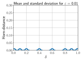
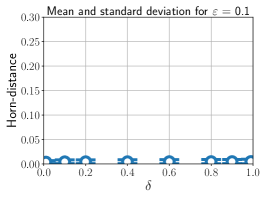
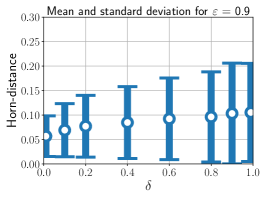
Figure 3: Horn-distances between the contexts from the BibSonomy data set and corresponding PAC bases for fixed $\varepsilon$ and varying $\delta$.

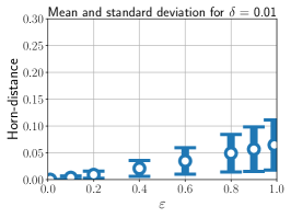
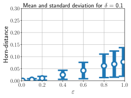
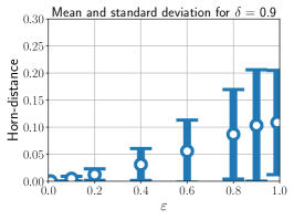
Figure 4: Horn-distance between the contexts from the BibSonomy data and corresponding PAC bases for fixed $\delta$ and varying $\varepsilon$.

This data set consists of a collection of 2835 formal contexts, each having exactly 12 attributes. It was created utilizing a data-dump from the BibSonomy platform, and a detailed description of how this had been done can be found in [8]. Those contexts have a varying number of objects and their canonical bases have sizes between one and 189.

Let us first fix the accuracy $\varepsilon$ and vary the confidence $\delta$ in order to investigate the influence of the latter. The mean value and the standard deviation over all 2835 formal contexts of the Horn-distance between the canonical basis and a PAC basis is shown in Figure 3. A first observation is that for all chosen values of $\varepsilon$, an increase of $1-\delta$ only yields a small change of the mean value, in most cases an increase as well. The standard deviation is, in almost all cases, also increasing. The results for the macro average of precision and recall are shown in Figure 5. Again, only a small impact on the final outcome when varying $1-\delta$ could be observed. We therefore omitted to show these in favor of the following plots.

Dually, let us now fix the confidence $\delta$ and vary the accuracy $\varepsilon$. The Horn-distances between the canonical basis and a computed PAC basis for this experiment are shown in Figure 4. From this we can learn numerous things. First, we see that increasing $\varepsilon$ always leads to a considerable increase in the Horn-distance, signaling that the PAC basis deviates more and more from the canonical basis. However, it is important to note that the mean values are always below $\varepsilon$, most times even significantly. Also, the increase for the Horn-distance while increasing $\varepsilon$ is significantly smaller than one. That is to say, the required accuracy bound is never realized, and especially for larger values of $\varepsilon$ the deviation of the computed PAC basis from the exact implicational theory is less than the algorithm would allow to. We observe a similar behavior for precision and recall. For small values of $\varepsilon$, both precision and recall are very high, i.e., close to one, and subsequently seem to follow an exponential decay.

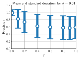
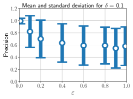
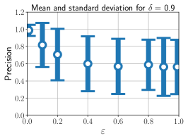
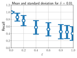
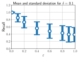
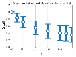
Figure 5: Measured precision (above) and recall (below) for fixed $\delta$ and varying $\varepsilon$ for the BibSonomy data set.

4.1.2 Artificial contexts

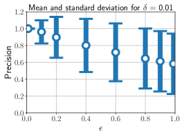
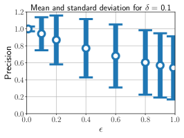
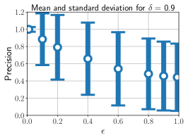
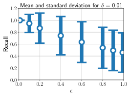
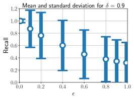
Figure 6: Measured recall for fixed $\varepsilon$ and varying $\delta$ (above) and fixed $\delta$ and varying $\varepsilon$ (below) for 3939 randomly generated formal contexts with ten attributes.

We now want to discuss the results of a computation analogous to the previous one, but with artificially generated formal contexts. For these formal contexts, the size of the attribute set is fixed at ten, and the number of objects and the density are chosen uniformly at random. The original data set consists of 4500 formal contexts, but we omit all that have a canonical basis with fewer than ten implications, to eliminate the high impact a single false implication in bases of small cardinality would have.

A selection of the experimental results is shown in Figure 6. We limit the presentation to precision and recall only, since the previous experiments indicate that investigating Horn-distance does not yield any new insights. For $\varepsilon=0.01$ and $\delta-1=0.01$, the precision as well as the recall is almost exactly one (0.999), with a standard deviation of almost zero (0.003). When increasing $\varepsilon$, the mean values deteriorate analogously to the previous experiment, but the standard deviation increases significantly more.

4.1.3 Stability

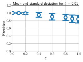
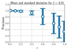
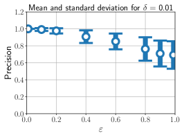
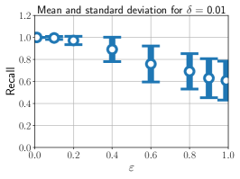
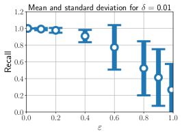
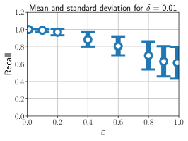
Figure 7: For fixed $\delta$ and varying $\varepsilon$, measured precision (above) and recall (below) stability for 100 runs on the same formal context with eight (left), nine (middle), and ten (right) attributes.

In our final experiment, we want to consider the impact of the randomness of the pac-basis algorithm when computing bases of fixed formal contexts. To this end, we shall consider particular formal contexts $\mathbb{K}$ and repeatedly compute probably approximately correct implication bases of $\mathbb{K}$. For these bases, we again compute recall and precision as we did in the previous experiments.

We shall consider three different artificial formal contexts with eight, nine, and ten attributes, and canonical bases of size 31, 40, and 70, respectively. In Figure 7, we show the precision and recall values for these contexts when calculating PAC bases 100 times. In general, the standard-deviation of precision and recall for small values of $\varepsilon$ are low. Increasing this parameter leads to an exponential decay of precision and recall, as expected, and the standard-deviation increases as well. We expect that both the decay of the mean value as well as the increase in standard deviation are less distinct for formal contexts with large canonical bases.

4.1.4 Discussion

Altogether the experiments show promising results. However, there are some peculiarities to be discussed. The impact of $1-\delta$ for Horn-distance in the case of the BibSonomy data set was considerably low. At this point, it is not clear whether this is due to the nature of the chosen contexts or to the fact that the algorithm is less constrained by $\delta$. The results presented in Figure 5 show that neither precision nor recall are impacted by varying $1-\delta$ as well. All in all, for the formal contexts of the BibSonomy data set, the algorithm delivered solid results in terms of accuracy and confidence, in particular when considering precision and recall, see Figure 5. Both measures indicate that the PAC bases perform astonishingly well, even for high values of $\varepsilon$.

For the experiment of the artificial contexts, the standard deviation increases significantly more than in the BibSonomy experiment. The source for this could not be determined in this work and needs further investigation. The overall inferior results for the artificial contexts, in comparison to the results for the BibSonomy data set, may be credited to the fact that many of the artificial contexts had a small canonical basis between 10 and 30. For those, a small amount of false or missing implications had a great impact on precision and recall. Nevertheless, the promising results for small values of $\varepsilon$ back the usability of the PAC basis generating algorithm.

4.2 A Small Case-Study

Let us consider a classical example, namely the Star-Alliance context [17], consisting of the members of the Star Alliance airline alliance prior to 2002, together with the regions of the world they fly to. The formal context $\mathbb{K}_{\mathsf{SA}}$ is given in Figure 8; it consists of 13 airlines and 9 regions, and $\operatorname{Can}(\mathbb{K}_{\mathsf{SA}})$ consists of 13 implications.

$$\begin{array}[]{l|*{9}{c}}\nobreak\leavevmode&\rotatebox{90.0}{\text{$\mathsf{Latin\ America}$}}&\rotatebox{90.0}{\text{$\mathsf{Europe}$}}&\rotatebox{90.0}{\text{$\mathsf{Canada}$}}&\rotatebox{90.0}{\text{$\mathsf{Asia\ Pacific}$}}&\rotatebox{90.0}{\text{$\mathsf{Middle\ East}$}}&\rotatebox{90.0}{\text{$\mathsf{Africa}$}}&\rotatebox{90.0}{\text{$\mathsf{Mexico}$}}&\rotatebox{90.0}{\text{$\mathsf{Caribbean}$}}&\rotatebox{90.0}{\text{$\mathsf{United\ States}$}}\\ \hline\cr\text{Air Canada}&\times&\times&\times&\times&\times&&\times&\times&\times\\ \text{Air New Zealand}&&\times&&\times&&&&&\times\\ \text{All Nippon Airways}&&\times&&\times&&&&&\times\\ \text{Ansett Australia}&&&&\times&&&&&\\ \text{The Austrian Airlines Group}&&\times&\times&\times&\times&\times&&&\times\\ \text{British Midlands}&&\times&&&&&&&\\ \text{Lufthansa}&\times&\times&\times&\times&\times&\times&\times&&\times\\ \text{Mexicana}&\times&&\times&&&\times&\times&\times\\ \text{Scandinavian Airlines}&\times&\times&&\times&&\times&&&\times\\ \text{Singapore Airlines}&&\times&\times&\times&\times&\times&&&\times\\ \text{Thai Airways International}&\times&\times&&\times&&&&\times&\times\\ \text{United Airlines}&\times&\times&\times&\times&&&\times&\times&\times\\ \text{VARIG}&\times&\times&&\times&&\times&\times&&\times\\ \end{array}$$

Figure 8: Star-Alliance Context $\mathbb{K}_{\mathsf{SA}}$

In the following, we shall investigate PAC bases of $\mathbb{K}_{\mathsf{SA}}$ and compare them to $\operatorname{Can}(\mathbb{K}_{\mathsf{SA}})$. Note that due to the probabilistic nature of this undertaking, it is hard to give certain results, as the outcomes of pac-basis can be different on different invocations, as seen in Section 4.1.3. It is nevertheless illuminating to see what results are possible for certain values of the parameters $\varepsilon$ and $\delta$. In particular, we shall see that implications returned by pac-basis are still meaningful, even if they are not valid in $\mathbb{K}_{\mathsf{SA}}$.

As a first case, let us consider comparably small values of accuracy and confidence, namely $\varepsilon=0.1$ and a $\delta=0.1$. For those values we obtained a basis $\mathcal{H}_{0.1,0.1}$ that differs from $\operatorname{Can}(\mathbb{K}_{\mathsf{SA}})$ only in the implication

$$\mathsf{Africa},\mathsf{Asia\ Pacific},\mathsf{Europe},\mathsf{United\ States},\mathsf{Canada}\to\mathsf{Middle\ East}$$

being replaced by

$$\mathsf{Africa},\mathsf{Latin\ America},\mathsf{Asia\ Pacific},\mathsf{Mexico},\mathsf{Europe},\mathsf{United\ States},\mathsf{Canada}\to\bot$$ (2)

Indeed, for the second implication to be refuted by the algorithm, the only counterexample in $\mathbb{K}_{\mathsf{SA}}$ would have been Lufthansa, which does not fly to the Caribbean. However, in our particular run of pac-basis that produced $\mathcal{H}_{0.1,0.1}$, this counterexample had not been considered, resulting in the implication from Equation (2) to remain in the final basis. Thus, while $\mathcal{H}_{0.1,0.1}$ does not coincide with $\operatorname{Can}(\mathbb{K}_{\mathsf{SA}})$, the only implication in which they differ (2) still has very high confidence in $\mathbb{K}_{\mathsf{SA}}$, in the sense of the usual notions of support and confidence of association rules [2]. Therefore, the basis $\mathcal{H}_{0.1,0.1}$ can be considered as a good approximation of $\operatorname{Can}(\mathbb{K}_{\mathsf{SA}})$.

As in the previous section, it turns out that increasing the parameter $\delta$ to values larger than $0.1$ does not change much of resulting basis. This is to be expected, since $\delta$ is a bound on the probability that the basis returned by pac-basis is not of accuracy $\varepsilon$. Indeed, even for as large a value as $\delta=0.8$, the resulting basis we obtained in our run of pac-basis was exactly $\operatorname{Can}(\mathbb{K}_{\mathsf{SA}})$. Nevertheless, care must be exercised when increasing $\delta$, as this increases the chance that pac-basis returns a basis that is far off from the actual canonical basis – if not in this run, then maybe in a latter one.

Conversely to this, and in accordance to the results of the previous section, increasing $\varepsilon$, and thus decreasing the bound on the accuracy, does indeed have a notable impact on the resulting basis. For example, for $\varepsilon=0.5$ and $\delta=0.1$, our run of pac-basis returned the basis

$$({\mathsf{Caribbean}}\to\bot),\ ({\mathsf{Asia\ Pacific},\mathsf{Mexico}}\to\bot),\ ({\mathsf{Asia\ Pacific},\mathsf{Europe}}\to\bot),$$

$$({\mathsf{Middle\ East}}\to\bot),\ ({\mathsf{Latin\ America}}\to{\mathsf{Mexico},\mathsf{United\ States},\mathsf{Canada}}).$$

While this basis enjoys a small Horn-distance to $\operatorname{Can}(\mathbb{K}_{\mathsf{SA}})$ of around 0.11, it can hardly be considered usable, as it ignores a great deal of objects in $\mathbb{K}_{\mathsf{SA}}$. Changing the confidence parameter $\delta$ to smaller or larger values again did not change much of the appearance of the bases.

To summarize, for our example context $\mathbb{K}_{\mathsf{SA}}$, we have seen that low values of $\varepsilon$ often yield bases that are very close to the canonical basis of $\mathbb{K}_{\mathsf{SA}}$, both intuitively and in terms of Horn-distance to the canonical basis of $\mathbb{K}_{\mathsf{SA}}$. However, the larger the values of $\varepsilon$ get, the less useful bases returned by pac-basis appear to be. On the other hand, varying the value for the confidence parameter $\delta$ within certain reasonable bounds does not seem to influence the results of pac-basis very much.

5 Summary and Outlook

The goal of this work is to give first evidence that probably approximately correct implication bases are a practical substitute for their exact counterparts, possessing advantageous algorithmic properties. To this end, we have argued both quantitatively and qualitatively that PAC bases are indeed close approximations of the canonical basis of both artificially generated as well as real-world data sets. Moreover, the fact that PAC bases can be computed in output-polynomial time alleviates the usual long running times of algorithms computing implication bases, and renders the applicability on larger data sets possible.

To push forward the usability of PAC bases, more studies are necessary. Further investigating the quality of those bases on real-world data sets is only one concern. An aspect not considered in this work is the actual running time necessary to compute PAC bases, compared to the one for the canonical basis, say. To make such a comparison meaningful, a careful implementation of the pac-basis algorithm needs to be devised, taking into account aspects of algorithmic design that are beyond the scope of this work.

We also have not considered relationships between PAC bases and existing ideas for extracting implicational knowledge from data. For example, in our investigation of Section 4.2, it turned out that implications extracted by the algorithm enjoy a high confidence in the data set. One could conjecture that there is a deeper connection between PAC bases and the notions of support and confidence of implications. It is also not too far fetched to imagine a notion of PAC bases that incorporates support and confidence right from the beginning.

The classical algorithm to compute the canonical basis of a formal context can easily be extended to the algorithm of attribute exploration. This algorithm, akin to query learning, aims at finding an exact representation of an implication theory that is only accessible through a domain expert. As the algorithm for computing the canonical basis can be extended to attribute exploration, we are certain that it is also possible to extend the pac-basis algorithm to a form of probably approximately correct attribute exploration. Such an algorithm, while not being entirely exact, would be highly sufficient for the inherently erroneous process of learning knowledge from human experts, while possibly being much faster. On top of that, existing work in query learning handling non-omniscient, erroneous, or even malicious oracles could be extended to attribute exploration so that it could deal with erroneous or malicious domain experts. In this way, attribute exploration could be made much more robust for learning tasks in the world wide web.

Acknowledgments: Daniel Borchmann gratefully acknowledges support by the Cluster of Excellence “Center for Advancing Electronics Dresden” (cfAED). The computations presented in this paper were conducted by conexp-clj, a general purpose software for formal concept analysis (https://github.com/exot/conexp-clj).

References

- [1] Kira Adaricheva and James B. Nation “Discovery of the D-basis in binary tables based on hypergraph dualization” In Theoretical Computer Science 658 Elsevier BV, 2017, pp. 307–315 DOI: 10.1016/j.tcs.2015.11.031
- [2] Rakesh Agrawal, Tomasz Imielinski and Arun N. Swami “Mining Association Rules between Sets of Items in Large Databases” In Proceedings of the ACM SIGMOD International Conference on Management of Data, 1993, pp. 207–216
- [3] Dana Angluin “Queries and concept learning” In Machine Learning 2.4 Springer Nature, 1988, pp. 319–342 DOI: 10.1007/bf00116828
- [4] Dana Angluin, Michael Frazier and Leonard Pitt “Learning conjunctions of Horn clauses” In Machine Learning 9.2-3 Springer Nature, 1992, pp. 147–164 DOI: 10.1007/bf00992675
- [5] Marta Arias and José L. Balcázar “Construction and learnability of canonical Horn formulas” In Machine Learning 85.3 Springer Nature, 2011, pp. 273–297 DOI: 10.1007/s10994-011-5248-5
- [6] Mikhail A. Babin “Models, Methods, and Programs for Generating Relationships from a Lattice of Closed Sets”, 2012
- [7] Daniel Borchmann “Learning terminological knowledge with high confidence from erroneous data.”, 2014
- [8] Daniel Borchmann and Tom Hanika “Some Experimental Results on Randomly Generating Formal Contexts.” In Proceedings of the 13th International Conference on Concept Lattices and their Applications (CLA 2016) 1624, CEUR Workshop Proceedings CEUR-WS.org, 2016, pp. 57–69 URL: http://dblp.uni-trier.de/db/conf/cla/cla2016.html#BorchmannH16
- [9] Bernhard Ganter “Two Basic Algorithms in Concept Analysis” In Proceedings of the 8th Interational Conference of Formal Concept Analysis 5986, Lecture Notes in Computer Science Springer, 2010, pp. 312–340
- [10] Bernhard Ganter and Sergei A. Obiedkov “Conceptual Exploration” Springer, 2016 DOI: 10.1007/978-3-662-49291-8
- [11] J.-L. Guigues and V. Duquenne “Famille minimale d’implications informatives résultant d’un tableau de données binaires” In Mathématiques et Sciences Humaines 24.95, 1986, pp. 5–18
- [12] Henry Kautz, Michael Kearns and Bart Selman “Horn approximations of empirical data” In Artificial Intelligence 74.1 Elsevier BV, 1995, pp. 129–145 DOI: 10.1016/0004-3702(94)00072-9
- [13] Francesco Kriegel and Daniel Borchmann “NextClosures: Parallel Computation of the Canonical Base” In Proceedings of the 12th International Conference on Concept Lattices and their Applications (CLA 2015) 1466, CEUR Workshop Proceedings Clermont-Ferrand, France: CEUR-WS.org, 2015, pp. 182–192
- [14] Sergei O. Kuznetsov “On the Intractability of Computing the Duquenne-Guigues Base” In Journal of Universal Computer Science 10.8, 2004, pp. 927–933
- [15] Sergei A. Obiedkov and Vincent Duquenne “Attribute-incremental construction of the canonical implication basis” In Annals of Mathematics and Artificial Intelligence 49.1-4, 2007, pp. 77–99
- [16] Uwe Ryssel, Felix Distel and Daniel Borchmann “Fast algorithms for implication bases and attribute exploration using proper premises” In Annals of Mathematics and Artificial Intelligence Special Issue 65 Springer, 2013, pp. 1–29
- [17] Gerd Stumme “Off to New Shores - Conceptual Knowledge Discovery and Processing” In International Journal on Human-Computer Studies (IJHCS) 59.3, 2003, pp. 287–325
- [18] Leslie G. Valiant “A Theory of the Learnable” In Communications of the ACM 27.11, 1984, pp. 1134–1142