A Three-loop Neutrino Model with Leptoquark Triplet Scalars

Abstract

We propose a three-loop neutrino mass model with a few leptoquark scalars in $SU(2)_{L}$-triplet form, through which we can explain the anomaly of $B\to K^{(*)}\mu^{+}\mu^{-}$, a sizable muon $g-2$ and a bosonic dark matter candidate, and at the same time satisfying all the constraints from lepton flavor violations. We perform global numerical analyses and show the allowed regions, in which we find somewhat restricted parameter space, such as the mass of dark matter candidate and various components of the Yukawa couplings in the model.

I Introduction

Recently, there was an $2.6\sigma$ anomaly in lepton-universality violation in the ratio $R_{K}\equiv B(B\to K\mu\mu)/B(B\to Kee)=0.745^{+0.090}_{-0.074}\pm 0.036$ by the LHCb Collaboration lhcb-2014 . In addition, sizable deviations were observed in angular distributions of $B\to K^{*}\mu\mu$ lhcb-2013 . The results can be interpreted by a large negative contribution to the Wilson coefficient $C_{9}$ of the semileptonic operator $O_{9}$, and also contributions to other Wilson coefficients, in particular to $C^{\prime}_{9}$ Descotes-Genon:2015uva ; Hiller:2014yaa ; Hiller:2016kry ; Descotes-Genon:2013wba .

The discrepancy between the theoretical prediction and experimental value on the muon anomalous magnetic dipole moment has been a long-standing problem, which stands at $3.6\sigma$ level with the deviation from the SM prediction at pdg .

$$\Delta a_{\mu}=a_{\mu}^{\rm exp}-a_{\mu}^{\rm SM}=288(63)(49)\times 10^{-11}.$$

If one insists on fulfilling the muon $g-2$ within $1\sigma-2\sigma$ of the experimental value in any models, it puts a strong constraint on the parameter space. For example, it requires a relatively light spectrum in the supersymmetric particles in the MSSM in order to bring the prediction to be within $1\sigma-2\sigma$ of the experimental value. A number of leptoquark models have been proposed to solve the $B\to K^{(*)}\mu\mu$ anomaly, but however it is very hard to satisfy simultaneously the muon $g-2$: see for example Ref. Cheung:2016fjo .

In this work, we propose a three-loop neutrino mass model with a few leptoquark scalars in $SU(2)_{L}$-triplet form. We attempt to use the model to explain the anomaly of $B^{(*)}\to K\mu^{+}\mu^{-}$, to achieve a sizable muon $g-2$, and to provide a bosonic dark matter candidate, and at the same time satisfying all the constraints from lepton flavor violations. The concrete model is based on the SM symmetry and a $Z_{2}$ symmetry as $SU(3)_{C}\times SU(2)_{L}\times U(1)_{Y}\times Z_{2}$. The model consists of the SM fields, 3 additional leptoquark triplet fields $\Delta_{1,2,3}^{a}$, and one colorless doublet scalar field $\eta$. These fields are assigned different $Z_{2}$ parities and hypercharges in such a way that each of the Yukawa-type couplings contributes to either neutrino mass, $B\to K^{(*)}\mu\mu$ anomaly, muon $g-2$, or the dark matter interactions. In this way, although the model contains more parameter, it can however explain all the above anomalies. The achievements of the model can be summarized in the following.

1. The neutrino mass pattern and oscillation can be accommodated with the Yukawa coupling terms $f,g,h$ in three-loop diagrams .

2. The Yukawa coupling term $f$ can give useful contributions to the Wilson coefficients $C_{9,10}$ in such a way that it can explain successfully the $B\to K^{(*)}\mu\mu$ anomaly.

3. The muon $g-2$ receives a large contribution from the Yukawa coupling term $r$. With some adjustment of the parameters a level of $10^{-9}$ is possible.

4. It provides a dark matter (DM) candidate $\eta_{R}$, the real part of the neutral component of the $\eta$ field with correct relic density.

5. The model can satisfy all the existing constraints from the lepton-flavor violations (LFVs), meson mixings, and rare $B$ decays.

This paper is organized as follows. In Sec. II, we describe the neutrino mass matrix and the solution to the anomaly in $b\to s\mu\bar{\mu}$. In Sec. III, we discuss various constraints of the model, including lepton-flavor violations, FCNC’s, oblique parameters, and dark matter. In Sec. IV, we present the numerical analysis and allowed parameter space, followed by the discussion on collider phenomenology. Sec. IV is devoted for conclusions and discussion.

II The Model

In this section, we describe the model setup, derive the formulas for the active neutrino mass matrix, and calculate the contributions to $b\to s\mu\bar{\mu}$.

	Quarks			Leptons		Vector Fermions
	$Q_{L_{i}}^{a}$	$u_{R_{i}}^{a}$	$d_{R_{i}}^{a}$	$L_{L_{i}}$	$e_{R_{i}}$	$L^{\prime}_{i}$
$SU(3)_{C}$	$\bm{3}$	$\bm{3}$	$\bm{3}$	$\bm{1}$	$\bm{1}$	$\bm{1}$
$SU(2)_{L}$	$\bm{2}$	$\bm{1}$	$\bm{1}$	$\bm{2}$	$\bm{1}$	$\bm{2}$
$U(1)_{Y}$	$\frac{1}{6}$	$\frac{2}{3}$	$-\frac{1}{3}$	$-\frac{1}{2}$	$-1$	$-\frac{1}{2}$
$Z_{2}$	$+$	$+$	$+$	$+$	$+$	$-$

Table 1: Field contents of fermions and their charge assignments under $SU(3)_{C}\times SU(2)_{L}\times U(1)_{Y}\times Z_{2}$, where the superscript (subscript) index $a\,(i)=1-3$ represents the color (flavor).

	$\Phi$	$\eta$	$\Delta_{1}^{a}$	$\Delta_{2}^{a}$	$\Delta_{3}^{a}$
$SU(3)_{C}$	$\bm{1}$	${\bm{1}}$	$\bm{3}$	$\bar{\bm{3}}$	$\bar{\bm{3}}$
$SU(2)_{L}$	$\bm{2}$	$\bm{2}$	$\bm{3}$	${\bm{3}}$	$\bm{3}$
$U(1)_{Y}$	$\frac{1}{2}$	$\frac{1}{2}$	$\frac{2}{3}$	$\frac{1}{3}$	$\frac{1}{3}$
$Z_{2}$	$+$	$-$	$-$	$-$	$+$

Table 2: Field contents of bosons and their charge assignments under $SU(3)_{C}\times SU(2)_{L}\times U(1)_{Y}\times Z_{2}$, where the superscript index $a=1-3$ represents the color.

II.1 Model setup

We show all the field contents and their charge assignments in Table 1 for the fermionic sector and in Table 2 for the bosonic sector.  Under this framework, the relevant part of the renormalizable Lagrangian and Higgs potential related to the neutrino masses are given by

$$-{\cal L} =y_{\ell_{i}}\bar{L}_{L_{i}}\Phi e_{R_{i}}+f_{ij}\bar{L}_{L_{i}}\Delta^{{\dagger}}_{3}(i\sigma_{2})Q^{c}_{L_{j}}+g_{ij}\bar{L}^{\prime}_{R_{i}}\Delta^{\dagger}_{1}Q_{L_{j}}+h_{ij}\bar{L}^{\prime}_{L_{i}}\Delta^{\dagger}_{2}Q^{c}_{L_{j}}+r_{ij}\bar{L}^{\prime}_{L_{i}}\eta e_{R_{j}}$$

$$+M_{i}\bar{L}^{\prime}_{L_{i}}L^{\prime}_{R_{i}}-\lambda_{0}\eta^{\dagger}\Delta_{3}\Delta_{1}\Phi^{*}-\lambda^{\prime}_{0}\eta^{\dagger}\Delta_{3}\Delta_{2}^{*}\Phi-\lambda_{5}(\eta^{\dagger}\Phi)^{2}+{\rm h.c.},$$ (II.1)

where we have defined $L^{\prime}\equiv[N,E]^{T}$, $\sigma_{2}$ is the second Pauli matrix and we have abbreviated the trivial terms for the Higgs potential. The scalar fields can be parameterized as

$$\Phi=\left[\begin{array}[]{c}0\\ \frac{v+\phi}{\sqrt{2}}\end{array}\right],\quad\eta=\left[\begin{array}[]{c}\eta^{+}\\ \frac{\eta_{R}+i\eta_{I}}{\sqrt{2}}\end{array}\right],\quad\Delta_{1}=\left[\begin{array}[]{cc}\frac{\delta_{2/3}^{(1)}}{\sqrt{2}}&\delta_{5/3}^{(1)}\\ \delta_{-1/3}^{(1)}&-\frac{\delta_{2/3}^{(1)}}{\sqrt{2}}\end{array}\right],$$ (II.8)

$$\Delta_{2}=\left[\begin{array}[]{cc}\frac{\delta_{1/3}^{(2)}}{\sqrt{2}}&\delta_{4/3}^{(2)}\\ \delta_{-2/3}^{(2)}&-\frac{\delta_{1/3}^{(2)}}{\sqrt{2}}\end{array}\right],\quad\Delta_{3}=\left[\begin{array}[]{cc}\frac{\delta_{1/3}^{(3)}}{\sqrt{2}}&\delta_{4/3}^{(3)}\\ \delta_{-2/3}^{(3)}&-\frac{\delta_{1/3}^{(3)}}{\sqrt{2}}\end{array}\right],$$ (II.13)

where the subscript next to the each field represents the electric charge of the field, $v=246$ GeV, and $\Phi$ is written in the form after the Goldstone fields are aboserbed as the longitudinal components of $W$ and $Z$ bosons. Notice here that each of the components of $\Delta_{3}$ and $\eta$ is in mass eigenstate, since there are no mixing terms that are assured by the $Z_{2}$ and $U(1)_{Y}$ symmetries. On the other hand, components of $\Delta_{1}$ and $\Delta_{2}$ can mix via $\Phi^{*}\Phi^{*}\Delta_{1}\Delta_{2}$ term. In the following analysis, we ignore such mixing effects assuming the relevant coupling is small.

Oblique parameters: Each of the mass components among $\Delta_{i}$ is strongly restricted by the oblique parameters. In order to evade such a strong constraint, we simply assume that each of the components should be of the same mass Cheung:2016frv . Thus, we define $m_{\Delta_{i}}$ as the mass for the components of $\Delta_{i}$. On the other hand, each component of $\eta$ cannot have the same mass, because the neutrino mass is proportional to the mass difference between the components of $\eta$, as you shall see later. Hence, we consider the oblique parameter constraints on $\eta$, which are characterized by $\Delta T$ and $\Delta S$. Their formulae are given by Barbieri:2006dq

$$\Delta T =\frac{F[\eta^{\pm},\eta_{I}]+F[\eta^{\pm},\eta_{R}]-F[\eta_{I},\eta_{R}]}{32\pi^{2}\alpha_{em}v^{2}},\ \Delta S=\frac{1}{2\pi}\int_{0}^{1}x(1-x)\ln\left[\frac{xm_{\eta_{R}}^{2}+(1-x)m_{\eta_{I}}^{2}}{m_{\eta^{\pm}}^{2}}\right],$$ (II.14)

where $\alpha_{em}\approx 1/137$ is the fine structure constant, and

$$F[a,b]=\frac{m_{a}^{2}+m_{b}^{2}}{2}-\frac{m_{a}^{2}m_{b}^{2}}{m_{a}^{2}-m_{b}^{2}}\ln\left[\frac{m_{a}^{2}}{m_{b}^{2}}\right],\ m_{a}\neq m_{b}.$$ (II.15)

The experimental bounds are given by pdg

$$(0.05-0.09)\leq\Delta S\leq(0.05+0.09),\quad(0.08-0.07)\leq\Delta T\leq(0.08+0.07).$$ (II.16)

We consider these constraints in the numerical analysis.

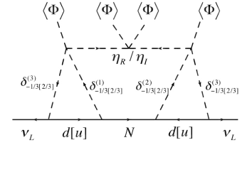
Figure 1: Neutrino mass matrix at the three-loop level, where we have two kind of diagrams that are running up-quarks and down quarks inside the loop.

Active neutrino mass matrix: The neutrino mass matrix is induced at three-loop level as shown in Fig. 1, and its formula is generally given by

$${\cal M}_{\nu_{ij}} ={\cal M}_{\nu_{ij}}^{d}+{\cal M}_{\nu_{ij}}^{u}+tr.,\ [{\cal M}_{\nu}^{u}=2{\cal M}_{\nu}^{d}(d\to u,\delta_{1/3}^{(i)}\to\delta_{2/3}^{(i)})],$$ (II.17)

$${\cal M}_{\nu_{ab}}^{d} =\frac{3^{2}\lambda_{0}\lambda^{\prime}_{0}(m_{R}^{2}-m_{I}^{2})v^{2}}{2\sqrt{2}(4\pi)^{6}M^{4}_{max}}\sum_{(a,b,c)=1}^{3}f_{ia}g^{T}_{ab}M_{b}h^{*}_{bc}f^{T}_{cj}F_{III}[r_{\Delta_{1}},r_{\Delta_{2}},r_{\Delta_{3}},r_{b},r_{R},r_{I},r_{d_{c}},r_{d_{a}}],$$ (II.18)

where we used the shorthand notation $m_{R/I}\equiv m_{\eta_{R/I}}$, and define $M_{\rm Max}\equiv$ Max[$M_{b},m_{\Delta_{i}},m_{R},m_{I}$], $r_{f}\equiv m_{f}^{2}/M_{\rm Max}^{2}$, and the three-loop function $F_{III}$ is given in the Appendix. Here we adopt an assumption $M_{max}=m_{\Delta_{3}}$, and require $1{\rm TeV}\lesssim m_{\Delta_{i}}$ (which suggests $x_{d},x_{u}\approx 0$), which is required by the direct bound on leptoquarks Cheung:2016frv . In this case, the neutrino mass matrix can be simplified as

$${\cal M}_{\nu_{ij}} \approx\frac{3^{3}\lambda_{0}\lambda^{\prime}_{0}(m_{R}^{2}-m_{I}^{2})v^{2}}{2\sqrt{2}(4\pi)^{6}m^{4}_{\Delta_{3}}}\left[fg^{T}(MF_{III})h^{*}f^{T}\right]_{ij}+tr.,$$ (II.19)

where we have abbreviated the symbol of summation and the argument of $F_{III}$. Then we derive the Yukawa coupling in terms of the experimental values and the parameters by introducing an arbitrary anti-symmetric matrix with complex values $A$ Okada:2015vwh , that is $A^{T}+A=0$, as follows:

$$g=\frac{1}{2}R^{-1}(h^{\dagger})^{-1}\left[f^{-1}V_{MNS}D_{\nu}V_{MNS}^{T}(f^{T})^{-1}+A\right]^{T},$$ (II.20)

$${\rm or}$$

$$h=\frac{1}{2}R^{*-1}(g^{\dagger})^{-1}\left[f^{-1}V_{MNS}D_{\nu}V_{MNS}^{T}(f^{T})^{-1}+A\right]^{*},$$ (II.21)

where we shall adopt the former formula in the numerical analysis below, and we define $D_{\nu}\equiv V_{MNS}^{T}{\cal M}_{\nu}V_{MNS}$ and parametrize as

$$R=\frac{3^{3}\lambda_{0}\lambda^{\prime}_{0}(m_{R}^{2}-m_{I}^{2})v^{2}MF_{III}}{2\sqrt{2}(4\pi)^{6}m^{4}_{\Delta_{3}}},\quad A\equiv\left[\begin{array}[]{ccc}0&a_{12}&a_{13}\\ -a_{12}&0&a_{23}\\ -a_{13}&-a_{23}&0\\ \end{array}\right].$$ (II.25)

Here we assume one massless neutrino (with normal ordering) in the numerical analysis below.

On the term $f$: The new physics contributions to account for the $B\to K^{(*)}\mu\mu$ anomaly lhcb-2013 can be interpreted as the shifts in the Wilson coefficients $C_{9,10}$. In our model, the relevant Wilson coefficients can be calculated as follows Cheung:2016frv :

$$(C_{9})^{\mu\mu} =-(C_{10})^{\mu\mu}=-\frac{1}{C_{\rm SM}}\frac{f_{b\mu}f_{s\mu}}{4m_{\Delta_{3}}^{2}},\quad C_{\rm SM}\equiv\frac{V_{tb}V^{*}_{ts}G_{F}\alpha_{\rm em}}{\sqrt{2}\pi},$$ (II.26)

where $m_{\Delta_{3}}\equiv m_{\delta_{4/3}^{(3)}}$, ${\rm G_{F}}\approx 1.17\times 10^{-5}$ GeV^-2 is the Fermi constant. We can then compare them to the best-fit values of $C_{9,10}$ from a global analysis based on the LHCb data in Ref. Descotes-Genon:2015uva as

$$C_{9}=-C_{10}:\ -0.68\;.$$ (II.27)

Here we also have to work within the $-0.75\lesssim C_{9}\lesssim-0.35$ in order to satisfy the the LHCb measurement of $R_{K}=B(B^{+}\to K^{+}\mu^{+}\mu^{-})/B(B^{+}\to K^{+}e^{+}e^{-})=0.745^{+0.090}_{-0.074}\pm 0.036$, which shows a $2.6\sigma$ deviation from the SM prediction Cheung:2016frv . Notice here that various constraints arising from the $f$ term include $B_{d/s}\to\ell^{+}\ell^{-}$, $\ell_{i}\to\ell_{j}\gamma$, which were given in Refs. Cheung:2016frv and Cheung:2016fjo , and we consider these constraints in the current numerical analysis. Although the muon $g-2$ is also induced from this term, the typical order is $10^{-12}\sim 10^{-13}$ with a negative sign Cheung:2016frv . Thus, we neglect this contribution to the muon $g-2$.

On the terms $g$ and $h$: The main constraint on $g$ and $h$ comes from $B(b\to s\gamma)$. The partial decay width for $b\to s\gamma$ is given by

$$\Gamma(b\to s\gamma)\approx\frac{3\alpha_{em}m_{b}^{5}}{4(4\pi)^{4}}\left|\frac{g^{\dagger}_{2a}g_{a3}}{2}F_{bs\gamma}[\delta_{2/3}^{(1)},a]-h^{\dagger}_{3a}h_{a2}\left(\frac{5}{3}F_{bs\gamma}[a,\delta_{1/3}^{(2)}]+F_{bs\gamma}[\delta_{1/3}^{(2)},a]\right)\right|^{2},$$ (II.28)

$$F_{bs\gamma}[a,b]=\frac{2m_{a}^{6}+3m_{a}^{4}m_{b}^{2}-6m_{a}^{2}m_{b}^{4}+m_{b}^{6}+12m_{a}^{4}m_{b}^{2}\ln[m_{b}/m_{a}]}{12(m_{a}^{2}-m_{b}^{2})^{4}},$$ (II.29)

then the branching ratio and its experimental bound Lees:2012wg are given by

$$B(b\to s\gamma)\approx \frac{\Gamma(b\to s\gamma)}{\Gamma_{tot.}}\lesssim 3.29\times 10^{-4}\;,$$ (II.30)

where $\Gamma_{tot.}\approx 4.02\times 10^{-13}$ GeV is the total decay width of the bottom quark. In our numerical analysis, we consider this constraint only for the $g$ and $h$ terms.

On the term $r$: This term is very important in our model because it can induce a large contribution to the muon $g-2$ and explain the relic density of dark matter (DM) if we assume the $\eta_{R}$ to be the DM candidate. First of all, let us consider the LFVs processes, $\ell_{a}\to\ell_{b}\gamma$, via one-loop diagrams. The branching ratio is given by

$$B(\ell_{a}\to\ell_{b}\gamma)=\frac{48\pi^{3}C_{ab}\alpha_{\rm em}}{{\rm G_{F}^{2}}m_{a}^{2}}(|(a_{R})_{ab}|^{2}+|(a_{L})_{ab}|^{2}),$$ (II.31)

where $m_{a(b)}$ is the mass for the charged-lepton eigenstate, $C_{ab}\approx(1,0.1784,0.1736)$ for $(a,b)=(2,1),(3,1),(3,2)$, and $a_{L(R)}$ is simply given by

$$(a_{L(R)})_{ab}\approx\sum_{i=1}^{3}\frac{r^{\dagger}_{bi}r_{ia}m_{a}}{(4\pi)^{2}}\left(F_{lfv}^{L(R)}[N_{i},\eta^{\pm}]-\frac{1}{2}F_{lfv}^{L(R)}[\eta_{I},E_{i}]-\frac{1}{2}F_{lfv}^{L(R)}[\eta_{R},E_{i}]\right),$$ (II.32)

$$F_{lfv}^{L}[a,b]=\frac{m_{a}^{4}+2m_{a}^{2}m_{b}^{2}+2m_{b}^{2}(m_{a}^{2}+m_{b}^{2})\ln\left(\frac{m_{b}^{2}}{m_{a}^{2}+m_{b}^{2}}\right)}{6m_{a}^{6}},\ F_{lfv}^{R}[a,b]=\frac{m_{a}^{2}+m_{b}^{2}\ln\left(\frac{m_{b}^{2}}{m_{a}^{2}+m_{b}^{2}}\right)}{6m_{a}^{4}},$$ (II.33)

where the mass of $E(N)_{a}$ is defined by $M_{E(N)_{a}}$. Current experimental upper bounds are given by TheMEG:2016wtm ; Adam:2013mnn

$$B(\mu\rightarrow e\gamma) \leq 4.2\times 10^{-13},\quad B(\tau\rightarrow\mu\gamma)\leq 4.4\times 10^{-8},\quad B(\tau\rightarrow e\gamma)\leq 3.3\times 10^{-8}~{}.$$ (II.34)

Muon $g-2$: The muon anomalous magnetic moment is simply given by $\Delta a_{\mu}\approx-m_{\mu}[a_{L}+a_{R}]_{22}$ in Eq. (II.33). Experimentally, it has been measured with a high precision, and its deviation from the SM prediction is $\Delta a_{\mu}={\cal O}(10^{-9})$ g-2 . It would be worth mentioning a new contribution to the leptonic decay of the $Z$ boson. In our case, the $Z$ boson can decay into a pair of charged leptons with a correction at one-loop level, and it is proportional to the Yukawa couplings related to the muon $g-2$. Therefore it can be enhanced due to the large Yukawa couplings. However, we have checked that this mode is within the experimental bound: $B(Z\to\ell\bar{\ell})\lesssim 3\times 10^{-2}$.

$Q-\bar{Q}$ mixing: The forms of $K^{0}-\bar{K}^{0}$, $B_{d}^{0}-\bar{B}_{d}^{0}$, and $D^{0}-\bar{D}^{0}$ mixings are, respectively, given by

$$\Delta m_{K} \approx\frac{1}{(4\pi)^{2}}\sum_{i,j=1}^{3}\left[g_{i2}g^{\dagger}_{1i}g^{\dagger}_{1j}g_{j2}\left(F^{K}_{box}[N_{i},N_{j},\delta_{1/3}^{(1)}]+\frac{F^{K}_{box}[E_{i},E_{j},\delta_{2/3}^{(1)}]}{4}\right)\right.$$

$$+\left.f_{i1}^{\dagger}f_{2i}f_{2j}f^{\dagger}_{j1}\left(F^{K}_{box}[\ell_{i},\ell_{j},\delta_{4/3}^{(3)}]+\frac{F^{K}_{box}[\nu_{i},\nu_{j},\delta_{1/3}]}{4}\right)\right.$$

$$+\left.h_{i1}^{\dagger}h_{2i}h_{2j}h^{\dagger}_{j1}\left(F^{K}_{box}[E_{i},E_{j},\delta_{4/3}^{(2)}]+\frac{F^{K}_{box}[N_{i},N_{j},\delta_{1/3}^{(2)}]}{4}\right)\right]\lesssim 3.48\times 10^{-15}[{\rm GeV}],$$ (II.35)

$$\Delta m_{B_{d}} \approx\frac{1}{(4\pi)^{2}}\sum_{i,j=1}^{3}\left[g_{i3}g^{\dagger}_{1i}g^{\dagger}_{1j}g_{j3}\left(F^{B}_{box}[N_{i},N_{j},\delta_{1/3}^{(1)}]+\frac{F^{B}_{box}[E_{i},E_{j},\delta_{2/3}^{(1)}]}{4}\right)\right.$$

$$+\left.f_{i3}^{\dagger}f_{1i}f_{1j}f^{\dagger}_{j3}\left(F^{B}_{box}[\ell_{i},\ell_{j},\delta_{4/3}^{(3)}]+\frac{F^{B}_{box}[\nu_{i},\nu_{j},\delta_{1/3}]}{4}\right)\right.$$

$$+\left.h_{i3}^{\dagger}h_{1i}h_{1j}h^{\dagger}_{j3}\left(F^{B}_{box}[E_{i},E_{j},\delta_{4/3}^{(2)}]+\frac{F^{B}_{box}[N_{i},N_{j},\delta_{1/3}^{(2)}]}{4}\right)\right]\lesssim 3.36\times 10^{-13}[{\rm GeV}],$$ (II.36)

$$\Delta m_{D} \approx\frac{1}{(4\pi)^{2}}\sum_{i,j=1}^{3}\left[g_{i2}g^{\dagger}_{1i}g^{\dagger}_{1j}g_{j2}\left(F^{D}_{box}[E_{i},E_{j},\delta_{5/3}^{(1)}]+\frac{F^{D}_{box}[N_{i},N_{j},\delta_{2/3}^{(1)}]}{4}\right)\right.$$

$$+\left.f_{i1}^{\dagger}f_{2i}f_{2j}f^{\dagger}_{j1}\left(F^{D}_{box}[\ell_{i},\ell_{j},\delta_{4/3}^{(3)}]+\frac{F^{D}_{box}[\nu_{i},\nu_{j},\delta_{1/3}]}{4}\right)\right.$$

$$+\left.h_{i1}^{\dagger}h_{2i}h_{2j}h^{\dagger}_{j1}\left(F^{D}_{box}[N_{i},N_{j},\delta_{2/3}^{(2)}]+\frac{F^{D}_{box}[E_{i},E_{j},\delta_{1/3}^{(2)}]}{4}\right)\right]\lesssim 6.25\times 10^{-15}[{\rm GeV}],$$ (II.37)

$$F^{Q}_{box}(x,y,z)=\frac{5m_{Q}f_{Q}^{2}}{24}\left(\frac{m_{Q}}{m_{q_{1}}+m_{q_{2}}}\right)^{2}\int\frac{\delta(1-a-b-c-d)dadbdcdd}{[am_{x}^{2}+bm_{y}^{2}+(c+d)m_{z}^{2}]^{2}},$$ (II.38)

where $(q_{1},q_{2})$ are respectively $(d,s)$ for $K$, $(b,d)$ for $B$, and $(u,c)$ for $D$. Each of the last inequalities in Eqs.(II.35 – II.37) represents the upper bound on the corresponding experimental value pdg . Here we used $f_{K}\approx 0.156$ GeV, $f_{B}\approx 0.191$ GeV, $m_{K}\approx 0.498$ GeV, and $m_{B}\approx 5.280$ GeV.

Dark Matter: Here we identify $\eta_{R}$ as the DM candidate, and denote its mass by $m_{R}\equiv M_{X}$. Direct detection: We have a Higgs portal contribution to the DM-nucleon scattering process, which is constrained by direct detection search such as the LUX experiment Akerib:2016vxi . Its spin independent cross section is simply given by Baek:2016kud

$$\sigma_{N}\approx 2.12\times 10^{-42}\times\left(\frac{(\lambda_{3}+\lambda_{4}+2\lambda_{5})v}{M_{X}}\right)^{2}[{\rm cm}]^{2},$$ (II.39)

where $\lambda_{3}$ and $\lambda_{4}$ are quartic couplings proportional to $(\eta^{\dagger}\eta)(\Phi^{\dagger}\Phi)$ and $(\eta^{\dagger}\Phi)(\Phi^{\dagger}\eta)$, respectively. The current experimental minimal bound is $\sigma_{N}\lesssim 2\times 10^{-46}$ cm² at $M_{X}\approx 50$ GeV. Once we apply this bound on our model, we obtain $\lambda_{3}+\lambda_{4}+2\lambda_{5}\lesssim 2\times 10^{-3}$. Hence we assume that all the Higgs couplings are small enough to satisfy the constraint, and we neglect DM annihilation modes via Higgs portal in estimating the relic density below. Notice here that photon and Z boson fields transform as $V_{\mu}\to-V^{\mu}$ under charge-parity ($CP$) conjugation, while $X$ is $CP$-even. Thus $X-X-\gamma(Z)$ couplings are not allowed because they violates the $CP$ invariance.
Relic density: We consider parameter region in which the DM annihilation cross section is $d$-wave dominant and the dark matter particles annihilate into a pair of charged-leptons, via the process $\eta_{R}\eta_{R}\to\ell_{i}\bar{\ell}_{j}$ with an $E_{a}$ exchange. Notice that there exist annihilation modes such as $\eta_{R}\eta_{R}\to W^{+}W^{-}/2Z$ arising from the kinetic term. These modes require a DM mass heavier than at least $500$ GeV Hambye:2009pw in order to obtain the correct relic density where coannihilation processes should be included. This case is, however, not in favor of explaining the muon $g-2$ anomaly. Thus we assume that $M_{X}\lesssim 80$ GeV and $\eta_{R}\eta_{R}\to W^{+}W^{-}/2Z$ processes are not kinematically allowed. Then the relic density is simply given by

$$\Omega h^{2}\approx\frac{1.70\times 10^{7}x_{f}^{3}}{\sqrt{g^{*}}M_{P}d_{\rm eff}[{\rm GeV}]},\quad{d_{\rm eff}\approx\sum_{(i,j,a)=1}^{3}\frac{|r_{ia}r^{\dagger}_{a,j}|^{2}M_{X}^{6}}{120\pi(M_{E_{a}}^{2}+M_{X}^{2})^{4}},}$$ (II.40)

where $g^{*}\approx 100$, $M_{P}\approx 1.22\times 10^{19}$, $x_{f}\approx 25$. In our numerical analysis below, we use the current experimental range for the relic density: $0.11\leq\Omega h^{2}\leq 0.13$ Ade:2013zuv .

III Numerical analysis

As a first step, we perform the numerical analysis on the $r$ term since this term is independent of the other parameters. We prepare 25 million random sampling points for the relevant input parameters as follows:

$$M_{X}\in[1,{80}]\text{GeV},\ m_{I}\approx m_{\eta^{\pm}}\in[1.1\times M_{X}\,,{{200}}\,]\text{GeV},$$

$$M_{1}\in[1.1\times M_{X}\,,{330}\,]\text{GeV},\ M_{2}\in[M_{1}\,,600\,]\text{GeV},\ M_{3}\in[M_{2}\,,700\,]\text{GeV},$$

$$r^{\prime}\in[-9,\ln(4\pi)],$$ (III.1)

where we define $M_{i}\equiv M_{E_{i}}=M_{N_{i}}$($i=1-3$), $r_{ij}\equiv(\pm 1)\times 10^{r^{\prime}_{ij}}$ and the lower mass bound $1.1\times M_{X}$ is expected to forbid the coannihilation processes. Under such parameter ranges, we have found 246 allowed points, which are shown in Fig. 2 satisfying all the constraints including LFVs, oblique parameters, and invisible decay of $Z$ boson, as discussed before. The left panel shows the allowed region to be

$$25{\rm[GeV]}\lesssim M_{X}\lesssim 80{\rm[GeV]},\quad 70{\rm[GeV]}\lesssim m_{\eta^{\pm}}\lesssim 140{\rm[GeV]},$$ (III.2)

where the lower bound of $\eta^{\pm}$ comes from the LEP experiment Osland:2013sla ; Akeroyd:2016ymd . The right panel shows the correlation of $r_{12}$ versus $\Delta a_{\mu}$, where $r_{12}$ is the most relevant parameter to obtain the sizable muon $g-2$ and correct relic density of the DM. It suggests that a rather small $r_{12}$ is possible to achieve the range $10^{-9}\leq\Delta a_{\mu}\leq 2\times 10^{-9}$, but we need a large $r_{12}$ for the range $2\times 10^{-9}<\Delta a_{\mu}\leq 2-4\times 10^{-9}$.  

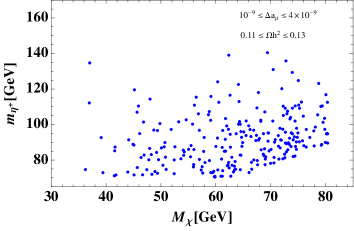
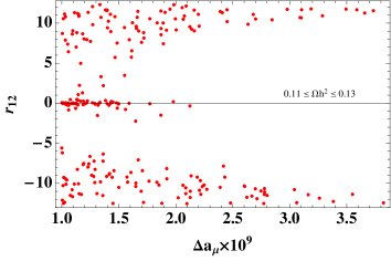
Figure 2: Scattering plots of the allowed parameter space sets to satisfy LFVs, oblique parameters, and invisible decay of $Z$ boson, in the plane of $M_{X}$-$m_{\eta^{\pm}}$ in the left panel; and in the plane of $\Delta a_{\mu}$-$r_{12}$ in the right panel, where $r_{12}$ is the most relevant parameter to obtain the sizable muon $g-2$ and relic density of DM.

In the next step, we attempt to find the parameter space points that can also solve the $B\to K^{(*)}\mu\mu$ anomaly by contributing to the $C_{9(10)}$, and at the same time satisfy all the constraints of the LFVs and FCNCs. Since the number of parameters is getting more and more, we are content with a benchmark point that we obtained in the first step. We prepare the benchmark point for the masses to fix the three-loop neutrino function $F_{III}$ as follows:

$$M_{X}\approx 54.26\ [{\rm GeV}],\quad m_{\eta_{I}}\approx m_{\eta^{\pm}}\approx 84.57\ [{\rm GeV}],$$ (III.3)

$$M_{1}\approx 277\ [{\rm GeV}],\quad M_{2}\approx 296\ [{\rm GeV}],\quad M_{3}\approx 401\ [{\rm GeV}],$$ (III.4)

$$m_{\Delta_{1}}\approx 1\ [{\rm TeV}],\quad m_{\Delta_{2}}\approx 1.1\ [{\rm TeV}],\quad m_{\Delta_{3}}\approx 1.2\ [{\rm TeV}],$$ (III.5)

where the above first two lines are provided by the first step so that $\Omega h^{2}\approx 0.120$ and $\Delta a_{\mu}\approx 2.67\times 10^{-9}$ are obtained with $r_{12}\approx-11.6$. The values in the last line are simply taken to evade the collider bound. To satisfy bound on the direct detection search, $\lambda_{3}+\lambda_{4}+2\lambda_{5}\lesssim 0.002$ is needed, where experimental upper bound is $\sigma_{I}\lesssim 2.2\times 10^{-46}$ cm², while $\lambda_{5}\approx 0.035$ that comes from $m_{\eta_{I}}^{2}-M_{X}^{2}=2\lambda_{5}v$. Therefore a little fine tuning is needed among $\lambda_{3},\lambda_{4},\lambda_{5}$. With this benchmark point, we have the following values:

$$F_{III}[x_{1}]\approx-108.68,\quad F_{III}[x_{2}]\approx-287.73,\quad F_{III}[x_{3}]\approx-317.11.$$ (III.6)

Also, we fix $-\lambda_{0}\lambda^{\prime}_{0}v^{2}/2\approx 1[{\rm GeV}^{2}]$ for simplicity. Then, we prepare 0.1 billion random sampling points for the following relevant input parameters:

$$[a_{12},a_{13},a_{23}]\in[-1-i,1+i]\times[10^{-3},1],\quad f^{\prime}\in[-3,\ln(4\pi)],\quad h^{\prime}\in[-3,\ln(4\pi)],$$ (III.7)

where we define $f(h)_{ij}\equiv(\pm 1)\times 10^{f^{\prime}(h^{\prime})_{ij}}$. In these parameter ranges, we have found 870 allowed points shown in Fig. 3, which satisfy all the constraints as discussed before. If we focus on the best-fit value of $C_{9}$, these figures show that the Yukawa couplings $f_{1j}(j=1-3)$ are very restricted as

$$|f_{11}|\lesssim{0.1},\quad|f_{12}|\lesssim{0.02},\quad|f_{13}|\lesssim{0.2},$$ (III.8)

where these coupling may affect the collider physics.

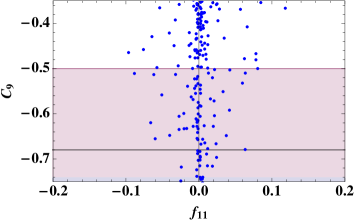
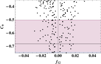
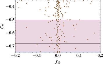
Figure 3: Scattering plots of the allowed parameter space sets in the plane of $(f_{1j})(j=1-3)$-$C_{9}$, where the horizontal line is the best fit value of $C_{9}=-0.68$. While the thin red region $[-0.85,-0.50]$ is the one at $1\sigma$ range. Notice here that we have taken the range $C_{9}\in[-0.75,-0.50]$ to satisfy $R_{K}$ at 1$\sigma$ confidential level Descotes-Genon:2015uva .

Collider Phenomenology: There are two types of new particles in this model other than the SM particles: leptoquarks $\Delta_{1,2,3}^{a}$ and a set of scalar bosons $\eta^{\pm,0}$ resulting from an isodoublet scalar field.

Note that $\Delta_{1,2}^{a}$ are assigned with $Z_{2}=-1$ while $\Delta_{3}^{a}$ are assigned with $Z_{2}=+1$. All $\Delta_{1,2,3}$ can be pair produced at hadronic colliders and being searched at the LHC. The direct search bound is roughly 1 TeV lhc-lq . On the other hand, only $\Delta_{3}^{a}$ can participate in the 4-fermion contact interaction, because of the $Z_{2}$ parity. The bound from the 4-fermion contact interaction was worked out in Ref. Cheung:2016frv ; Cheung:2016fjo that the bound is currently inferior to the direct search bound of about 1 TeV. Therefore, we shall use 1 TeV as the current bound on the $\Delta_{1,2,3}$ bosons.

The isodoublet field $\eta$ gives rise to a pair of charged bosons $\eta^{\pm}$, a scalar $\eta_{R}$, and a pseudoscalar $\eta_{I}$. The charged bosons $\eta^{\pm}$ can run in the triangular loop vertex of $H\gamma\gamma$. Nevertheless, we can suppress such effects by choosing the $\lambda_{5}$ term in Eq. (II.1) very small. As we have explained above such a term is small to avoid the conflict of the direct detection bound. Although the interaction between the $\eta$ field and the SM Higgs field is suppressed for the above reasons, the $\eta$ can still interact through the kinetic term as it has $SU(2)_{L}$ and $U(1)_{Y}$ interactions. We expect some typical interactions with the gauge bosons:

$$Z\eta^{+}\eta^{-},\;\;Z\eta_{R}\eta_{I},\;\;W^{+}\eta^{-}\eta_{R},\;\;{\rm etc}\;.$$

An interesting signature would be Drell-Yan type production of $\eta^{\pm}\eta_{R}$ via a virtual $W$. The $\eta^{\pm}$ decays into multi-leptons and $\eta_{R}$ via the virtual $L^{\prime}$ fields. Therefore, the final state consists of multi-charged-leptons and missing energies. Similarly, in the process $pp\to Z^{*}\to\eta_{R}\eta_{I}$, the $\eta_{I}$ would decay into $\eta_{R}$ eventually with a number of very soft leptons, which may not be detectable. Therefore, the best would be the one produced via virtual $W$.

IV Conclusions

We have investigated a three-loop neutrino mass model with some leptoquark scalars with $SU(2)_{L}$-triplet, in which we have explained the anomaly in $B\to K^{(*)}\mu^{+}\mu^{-}$, sizable muon $g-2$, bosonic dark matter, satisfying all the constraints such as LFVs, FCNCs, invisible decay, and so on. Then we have performed the global numerical analysis and shown the allowed region, in which we have found restricted parameter space, e.g.,

$$25{\rm[GeV]}\lesssim M_{X}\lesssim 80{\rm[GeV]},\quad 70{\rm[GeV]}\lesssim m_{\eta^{\pm}}\lesssim 140{\rm[GeV]},$$

$$|f_{11}|\lesssim{0.1},\quad|f_{12}|\lesssim{0.02},\quad|f_{13}|\lesssim{0.2}.$$

We find that $\sim O(100)$ GeV inert doublet scalar is preferred to obtain sizable muon $g-2$. Thus these light inert scalars could be tested by collider experiments such as LHC in which these scalars are produced via electroweak processes. The promising signature of our model comes from the process $pp\to W^{\pm}\to\eta^{\pm}\eta_{R}$ which provides signals of multi-leptons plus missing transverse momentum.

Appendix A Loop function

Here we show the explicit form of three-loop function $F_{III}$, which is given by

$$F_{III}=\int[dx_{i}]\frac{\delta(\sum_{i=1}^{5}x_{i}-1)(x_{2}-1)^{2}}{x_{1}^{2}}\int\frac{[dy_{i}]\delta(\sum_{i=1}^{3}y_{i}-1)}{[(1+y_{1})x_{1}x_{2}-x_{1}-x_{2}+1]^{3}}\int\frac{[dz_{i}]\delta(\sum_{i=1}^{3}z_{i}-1)z_{1}^{2}}{[y_{1}\Delta_{3}+z_{2}r_{\delta_{13}^{(2)}}+z_{3}r_{d_{a}}]^{3}},$$

$$\Delta_{3}=\frac{x_{2}-1}{x_{1}[(1+y_{1})x_{1}x_{2}-x_{1}-x_{2}+1]}\left(x_{1}r_{\delta_{13}^{(1)}}+x_{2}r_{\delta_{13}^{(2)}}+x_{3}r_{b}+x_{4}r_{\eta_{R}}+x_{5}r_{\eta_{I}}\right)$$

$$-\frac{x_{1}x_{2}}{A^{2}y_{1}[(1+y_{1})x_{1}x_{2}-x_{1}-x_{2}+1]}\left(y_{2}r_{\delta_{13}^{(3)}}+y_{3}r_{d_{c}}\right),$$

where $A\equiv x_{1}/(x_{2}-1)$, $[dx_{i}]\equiv\int_{0}^{1}dx_{1}\int_{0}^{1-x_{1}}dx_{2}\int_{0}^{1-x_{1}-x_{2}}dx_{3}\int_{0}^{1-x_{1}-x_{2}-x_{3}}dx_{4}$, $[dy_{i}]\equiv\int_{0}^{1}dy_{1}\int_{0}^{1-y_{1}}dy_{2}$, and $[dz_{i}]\equiv\int_{0}^{1}dz_{1}\int_{0}^{1-z_{1}}dz_{2}$.

References

- (1) R. Aaij et al. [LHCb Collaboration], Phys. Rev. Lett. 113, 151601 (2014) [arXiv:1406.6482 [hep-ex]].
- (2) R. Aaij et al. [LHCb Collaboration], Phys. Rev. Lett. 111, 191801 (2013) [arXiv:1308.1707 [hep-ex]].
- (3) S. Descotes-Genon, L. Hofer, J. Matias and J. Virto, JHEP 1606, 092 (2016) [arXiv:1510.04239 [hep-ph]].
- (4) G. Hiller and M. Schmaltz, Phys. Rev. D 90, 054014 (2014) [arXiv:1408.1627 [hep-ph]].
- (5) G. Hiller, D. Loose and K. Schonwald, JHEP 1612, 027 (2016) [arXiv:1609.08895 [hep-ph]].
- (6) S. Descotes-Genon, J. Matias and J. Virto, Phys. Rev. D 88, 074002 (2013) [arXiv:1307.5683 [hep-ph]].
- (7) K.A. Olive et al. (Particle Data Group), Chin. Phys. C, 38, 090001 (2014) and 2015 update.
- (8) K. Cheung, T. Nomura and H. Okada, arXiv:1610.02322 [hep-ph].
- (9) L. M. Krauss, S. Nasri and M. Trodden, Phys. Rev. D 67, 085002 (2003) [arXiv:hep-ph/0210389].
- (10) M. Aoki, S. Kanemura and O. Seto, Phys. Rev. Lett. 102, 051805 (2009) [arXiv:0807.0361].
- (11) M. Gustafsson, J. M. No and M. A. Rivera, Phys. Rev. Lett. 110, 211802 (2013) arXiv:1212.4806 [hep-ph].
- (12) C. S. Chen, K. L. McDonald and S. Nasri, Phys. Lett. B 734, 388 (2014) [arXiv:1404.6033 [hep-ph]].
- (13) K. Cheung, T. Nomura and H. Okada, arXiv:1610.04986 [hep-ph].
- (14) R. Barbieri, L. J. Hall and V. S. Rychkov, Phys. Rev. D 74, 015007 (2006) [hep-ph/0603188].
- (15) H. Okada and Y. Orikasa, Phys. Rev. D 94, no. 5, 055002 (2016) [arXiv:1512.06687 [hep-ph]].
- (16) J. P. Lees et al. [BaBar Collaboration], Phys. Rev. D 86, 052012 (2012) [arXiv:1207.2520 [hep-ex]].
- (17) A. M. Baldini et al. [MEG Collaboration], arXiv:1605.05081 [hep-ex].
- (18) J. Adam et al. [MEG Collaboration], Phys. Rev. Lett. 110, 201801 (2013) [arXiv:1303.0754 [hep-ex]].
- (19) Review by A. Hoecker and W.J. Marciano in PDG.
- (20) D. S. Akerib et al., arXiv:1608.07648 [astro-ph.CO].
- (21) S. Baek, T. Nomura and H. Okada, Phys. Lett. B 759, 91 (2016) [arXiv:1604.03738 [hep-ph]].
- (22) T. Hambye, F.-S. Ling, L. Lopez Honorez and J. Rocher, JHEP 0907, 090 (2009) Erratum: [JHEP 1005, 066 (2010)] [arXiv:0903.4010 [hep-ph]].
- (23) P. A. R. Ade et al. [Planck Collaboration], Astron. Astrophys. 571, A16 (2014) [arXiv:1303.5076 [astro-ph.CO]].
- (24) P. Osland, A. Pukhov, G. M. Pruna and M. Purmohammadi, JHEP 1304, 040 (2013) [arXiv:1302.3713 [hep-ph]].
- (25) A. G. Akeroyd et al., arXiv:1607.01320 [hep-ph].
- (26) See for example, M. Aaboud et al. [ATLAS Collaboration], New J. Phys. 18, no. 9, 093016 (2016) [arXiv:1605.06035 [hep-ex]].