Dynamic capillary phenomena using Incompressible SPH

Abstract

Grid based fluid simulation methods are not able to monolithically capture complex non-linear dynamics like the rupture of a dynamic liquid bridge between freely colliding solids, an exemplary scenario of capillary forces competing with inertial forces in engineering applications. We introduce a new Incompressible Smoothed Particle Hydrodynamics method for simulating three dimensional fluid-solid interaction flows with capillary (wetting and surface tension) effects at free surfaces. This meshless approach presents significant advantages over grid based approaches in terms of being monolithic and in handling interaction with free solids. The method is validated for accuracy and stability in dynamic scenarios involving surface tension and wetting. We then present three dimensional simulations of crown forming instability following the splash of a liquid drop, and the rupture of a liquid bridge between two colliding solid spheres, to show the method’s advantages in the study of dynamic micromechanical phenomena involving capillary flows.

1 Introduction

Appreciation of non-linear micro mechanical phenomena is crucial to advance the efficiency of many production processes that are aided by the presence of a momentary liquid phase. Processes such as wet fluidized beds [21], powder agglomeration [15], pelletizing [41] and spray painting [47] in industrial scales are essentially multiscale phenomena where the macroscopic behaviour is predicted by simulations using simple analytical models for the smaller scale mechanics. Improving the understanding of micromechanics using well resolved simulations is crucial to improve the models employed in macroscopic simulations. Dynamic capillary scenarios in small scales are difficult to study experimentally and traditional fluid simulation methods have their limitations and therefore there is an increasing interest in exploring meshless approaches.

Traditional multiphase flow simulation methods employing the Volume of fluid (VOF) method [14], Constraint interpolation method (CIP) [45], Level set or Coupled Level set VOF methods [40] are increasingly used to simulate such phenomena. However, they have their limitations in handling high density ratio or free surfaces [31], moving three-phase contact line consistent with a no-slip wall [33, 10] and interacting solids with all six degrees of freedom. While higher order consistency is easy to achieve in Eulerian methods, multi component simulations require coupling of different numerical approaches (for example, the Immersed Boundary Method [29]) limiting the ease of set up of these simulations.

Meshless Lagrangian simulation methods, for example the Smoothed Particle Hydrodynamics (SPH) and its derivatives, have the advantage of handling complex shaped free surfaces [23]—a better approximation to a typical liquid-air system than a finite density ratio and explicit interactions with solids [26, 27]. While free surfaces are implicitly handled by traditional SPH methods with a weak compressibility model, they require non-trivial treatment in case of the more accurate Incompressible SPH (ISPH) methods [19], which solves for a pressure field for strict incompressibility. An accurate semi-analytic free surface model for ISPH was implemented recently [26], expanding the scope of this more accurate version of SPH. Particularly, this approach allows finite pressure gradients close to the free surface making it possible to couple different interface tension models to the free surface.

Surface tension was initially implemented in SPH using a Continuum Surface Force (CSF) model[6, 24], following Eulerian two phase flow simulation methods [6]. Since then CSF based surface tension models in SPH have improved considerably in accuracy and stability [1, 7]. In CSF, the surface tension force is modeled as a volumetric force proportional to the interface curvature, which in turn is obtained by computation of divergence of a Heaviside step function [24] or by geometrically reconstructing the interface [48]. While the former is limited in its application to interfaces with fluid on both sides, the latter requires expensive computations to identify particles at the interface [48]. Inspired by the molecular origin of surface tension phenomena, a model based on pair-wise forces was introduced by [28] for a van der Waals liquid drop. This approach was further improved in [37] and applied to a number of free surface problems. Such approaches are also used in computer graphics research for emulating optically plausible behaviour with considerably less computational cost [3]. In a recent work [39], the relations between macroscopic parameters like surface tension coefficient and apparent contact angle to the strength and nature of the pairwise particle forces was elucidated. In this work, a number of validation cases were presented by the authors establishing the method as an accurate surface tension model of engineering importance.

In the present paper, we present a novel ISPH method that couples an accurate free surface model to a pairwise force capillary model to simulate dynamic capillary effects. The relation between inter particle force strengths and the macroscopic parameters like surface tension and contact angle are given for free surfaces. Different aspects of the method such as dynamics due to surface tension, contact angle, capillary force balance etc., are separately validated.

We then apply the method to the simulation of two three dimensional problems exemplary of dynamic capillary effects. First, we observe the onset of instability and the breaking of symmetry following splash of a drop on a liquid film. Second, we obtain the critical velocity for agglomeration of two colliding wet solids by observing the rupture of the liquid bridges as the solids depart and compare it with theoretical results.

2 ISPH Formulation

The governing equation and SPH discretization used for incompressible fluids with free surface is presented here. The philosophy and basic formulation of the SPH method can be found in a number of works, for example [42], and here we present only the SPH approximations that are relevant to the presented method.

2.1 Governing Equations

Momentum conservation equations for a Newtonian fluid are solved using the SPH method in an updated-Lagrangian frame of reference. By updated we mean that the reference configuration for application of constitutive relation of the material is updated with time, as opposed to a purely Lagrangian method where the reference configuration is a relaxed initial state. The Navier–Stokes equations governing the momentum conservation of incompressible isothermal flow are given by,

$$\frac{d\mathbf{u}}{dt}=\frac{1}{\rho}\left(-\nabla p+\nabla\cdot\left(2\mu\mathbf{D}\right)\right)+\mathbf{f}^{B},$$ (1)

where $\mathbf{u}$ is the velocity, $p$ is the pressure, $\rho$ is the density, $\mu$ is the coefficient of viscosity of the fluid, $\mathbf{D}=(\nabla\mathbf{u}+\nabla\mathbf{u}^{T})/2$ is the deformation rate tensor, $\mathbf{f}^{B}$ is the body force per unit mass on the fluid element and $t$ is the time. The Navier-Stokes equation has been written in the Lagrangian formulation and $d/dt$ denotes the material derivative. The mass conservation equation for incompressible flows is given by,

$$\nabla\cdot\mathbf{u}=0.$$ (2)

The governing equations are discretized on a particle domain in SPH. As a model for surface tension, a molecular dynamics inspired pairwise force model [39] is superimposed on the particle system following the observation that molecular forces are superposable on forces derived from momentum conservation equations on the same particle system [28].

2.2 SPH formulation

The SPH discretization of the governing equations (1) together with a pairwise force model [39] is as follows:

$$\begin{split}\left.\frac{d\mathbf{u}}{dt}\right|_{a}=&-\sum_{b}m_{b}\left(\frac{p_{a}}{\rho_{a}^{2}}+\frac{p_{b}}{\rho_{b}^{2}}\right)\nabla_{a}W_{ab}\\ &+\sum_{b}m_{b}\left(\frac{2\mu}{(\rho_{a}\rho_{b})}\frac{\mathbf{r}_{ab}\cdot\nabla W_{ab}}{r_{ab}^{2}+\epsilon^{2}}\right)\mathbf{u}_{ab}+\mathbf{f}^{\textrm{int}}_{a}+\mathbf{f}_{a}^{b},\end{split}$$ (3)

where $m$ is the mass, $\rho$ is the density, $p$ is the pressure, at a particle identified by the subscript $a$ or its neighbor $b$. Here $\mathbf{r}_{ab}$ is the displacement vector between particles $a$ and $b$ and $r_{ab}$, its magnitude. The function $W$ is the symmetric and positive definite smoothing function, also known as the kernel for the SPH discretization defined for a particle pair as $W_{ab}=W(r_{ab},h)$, where $h$ is the smoothing length of the kernel. The kernel has a compact support and its domain is cut off by a factor $q_{\textrm{cutoff}}$ times the smoothing length $h$ in space. The pairwise forces $\mathbf{f}_{ab}^{\textrm{int}}$, applied to simulate interfacial force is explained in Sec. 2.4 and $\mathbf{f}_{a}^{b}$ denotes the body force per unit mass acting on particle $a$ and represents the gravitational acceleration in the present work. We have used a viscous force approximation (the second term on the right hand side) that is extensively used in SPH literature [25]:

$$\nabla\cdot\left(\frac{\mu}{\rho}\nabla\mathbf{u}\right)_{a}=\sum_{b}m_{b}\left(\frac{\mu_{a}+\mu_{b}}{\rho_{a}\rho_{b}}\frac{\mathbf{r}_{ab}\cdot\nabla_{a}W_{ab}}{r_{ab}^{2}+\epsilon^{2}}\right)\mathbf{u}_{ab},$$ (4)

where $\mathbf{u}_{ab}$ is the relative velocity vector between particles $a$ and $b$, $\epsilon$ is a small positive number (usually chosen as $(0.01h)^{2}$) to avoid division by zero for a rare incident of particles overlapping each other, and a pressure gradient approximation (the first term on the right hand side) applicable to multiphase flow problems [8, 36]:

$$\left(\frac{\nabla p}{\rho}\right)_{a}=\sum_{b}m_{b}\frac{p_{a}+p_{b}}{\rho_{a}\rho_{b}}\nabla_{a}W_{ab}.$$ (5)

Near solid walls, the gradient and divergence approximations require a filled kernel neighborhood. This is achieved by distributing static particles along solid walls with the same particle spacing as in the initial spacing of fluid particles. These wall particles can be modelled as belonging to rigid bodies to simulate free solids interacting with the liquid. Such an approach conserves linear and angular momentum and can be seen by a force balance across the solid-liquid interface as explained in [26].

At free surfaces, standard weakly compressible SPH is known to naturally satisfy a zero pressure Dirichlet boundary condition corresponding to a moving interface [23] if a conservative pressure gradient (for example, eq. 5) approximation is used. However, explicit application of Dirichlet boundary condition is necessary if a pressure solver is invoked to compute the pressure field. It is important for the Dirichlet boundary condition to be applied in a consistent and accurate manner to preserve the accuracy of ISPH.

2.3 ISPH and the free surface formulation

Following grid based methods for incompressible flows, where a divergence free constraint is imposed on velocity field, ISPH solves for the pressure Poisson equation

$$\nabla\cdot\left(\frac{\nabla p}{\rho}\right)=-\frac{\nabla\cdot\mathbf{u}}{\Delta t},$$ (6)

on the particle domain. The SPH discretization of this equation [19] is:

$$\left.\nabla\cdot\left(\frac{\nabla p}{\rho}\right)\right|_{a}=\sum_{b}\frac{m_{b}}{\rho_{b}}\frac{4}{\rho_{a}+\rho_{b}}\left(P_{a}-P_{b}\right)\frac{\mathbf{r}_{ab}\cdot\nabla_{a}W_{ab}}{r_{ab}^{2}+\epsilon^{2}}.$$ (7)

When a linear system is solved on the particle domain to obtain pressure, application of Dirichlet boundary condition for pressure is necessary. A semi-analytic model was introduced in a previous work [26] to implement free surface Dirichlet boundary condition with greater accuracy and robustness over previous approaches involving identification of free surface particles [19, 43]. This model is implemented by modifying the linear system for solving the pressure Poisson equation in the SPH particle domain as:

$$\begin{split}\left.\nabla\cdot\left(\frac{\nabla p}{\rho}\right)\right|_{a}=&(p_{a}-p_{o})\kappa-\sum_{b_{i}}\frac{m_{b}}{\rho_{b}}\frac{4}{\rho_{a}+\rho_{b}}p_{b}\frac{\mathbf{r}_{ab}\cdot\nabla_{a}W_{ab}}{r_{ab}^{2}+\epsilon^{2}}\\ &+\sum_{b_{i}}\frac{m_{b}}{\rho_{b}}\frac{4}{\rho_{a}+\rho_{b}}p_{o}\frac{\mathbf{r}_{ab}\cdot\nabla_{a}W_{ab}}{r_{ab}^{2}+\epsilon^{2}}\end{split}$$ (8)

where $p_{0}$ represents the ambient pressure and $\kappa$, given by

$$\kappa=\sum_{b}\frac{m_{b}}{\rho_{b}}\frac{4}{\rho_{a}+\rho_{b}}\frac{\mathbf{r}_{ab}\cdot\nabla_{a}W_{ab}}{r_{ab}^{2}+\epsilon^{2}},$$ (9)

represents a kernel completion factor. Here, The derivation of both the above equations can be seen in [26]. In effect, this model simply modifies the terms in the leading diagonal of the linear system for pressure. The time integration of the field variables are performed by a velocity Verlet integration algorithm [4] given by:

$$\mathbf{r}_{a}(t+\Delta t) =\mathbf{r}_{a}(t)+\Delta t\mathbf{u}_{a}(t)+\frac{\Delta t^{2}}{2}\mathbf{f}^{\text{tot}}_{a}(t)$$ (10)

$$\mathbf{u}_{a}(t+\Delta t) =\mathbf{u}_{a}(t)+\frac{\Delta t}{2}\left(\mathbf{f}^{\text{tot}}_{a}(t)+\mathbf{f}^{\text{tot}}_{a}(t+\Delta t)\right).$$ (11)

Here, $\mathbf{f}^{\text{tot}}_{a}$ is the total acceleration of a particle $a$ contributed by both continuum (viscous, pressure, body forces) and inter-particle forces. The integration time step $\Delta t$ is set to satisfy the following constraint for numerical stability [39]:

$$\Delta t\leq\min_{a}\left(0.25\frac{h}{3|\mathbf{u}_{a}|},0.25\sqrt{\frac{m_{a}h}{3|\mathbf{f}^{\text{int}}_{a}|}},0.25\frac{\rho h^{2}}{9\mu}\right).$$ (12)

time integration and algorithm

2.4 Pairwise-force model for free surface ISPH

The pairwise force required to model capillary effects needs to be repulsive in the short range and attractive in the long range and may be much less stiffer than the potentials used in molecular dynamics simulations [35]. The inter-particle acceleration term that appears in eq. 3 is given by:

$$\mathbf{f}_{a}^{\textrm{int}}=\sum\limits_{b}\frac{F_{\alpha\beta}^{\textrm{int}}({r}_{ab})}{m_{a}}\frac{\mathbf{r}_{ab}}{r_{ab}},$$ (13)

where $\alpha$ and $\beta$ represent the phases of the particles $a$ and $b$, respectively, separated by a vector $\mathbf{r}_{ab}$ in space. The pairwise force magnitude as a function of displacement between particles is given as [37]:

$$F_{\alpha\beta}^{\textrm{int}}(r_{ab})=\begin{cases}-s_{\alpha\beta}\cos\left(\frac{3\pi}{4}q_{ab}\right)&q_{ab}=\frac{r_{ab}}{h}\leq q_{\textrm{cutoff}}\\ 0&q_{ab}=\frac{r_{ab}}{h}>q_{\textrm{cutoff}},\end{cases}$$ (14)

where $q_{\textrm{cutoff}}$ is the ratio of cut off length of the kernel to the smoothing length $h$. Here, we have chosen the cut off length of the kernel for SPH computation to be the same for the inter-particle forces. Also, $s_{\alpha\beta}$ is the interaction strength between particles of phases $\alpha$ and $\beta$ respectively. Symmetry in the strength ensures conservation of linear momentum between particles, ensuring conservation of linear momentum in the SPH discretization. The pairwise force based SPH model is becoming increasingly popular [37, 20, 38] in literature owing to its ease of application and robustness. In a recent work [39] a detailed explanation on how the macroscopic parameters such as surface tension, contact angle and the pressure resulting from pairwise forces, called the ‘virial pressure’ can be related to the strength of the pairwise forces is provided. This approach was also applied to free surface flows in earlier works [28, 37]. However the application has been limited to weakly compressible SPH solvers, since ISPH free surface flows . In the present work the pairwise force model is applied to the ISPH algorithm with the free surface treatment presented in the previous section.

The stress at a given point in a particle system with given pairwise forces can be computed according to the Hardy’s formula [35]. This formula is given as a sum of stress due to inter-particle forces and the convection of particles. In the present work, since a hydrodynamic governing equation is used to model the fluid, only the stress due to inter-particle forces becomes relevant, and is given by:

$$\mathbf{T}_{\textrm{int}}(x)=\frac{1}{2}\sum\limits_{a=1}^{N}\sum\limits_{b=1}^{N}\mathbf{f}_{ab}\otimes(\mathbf{r}_{a}-\mathbf{r}_{b})\int\limits_{0}^{1}\tilde{\psi}_{\eta}(\mathbf{x}-s\mathbf{r}_{a}-(1-s)\mathbf{r}_{b})ds,$$ (15)

where the function $\tilde{\psi}$ is a weighting function with a compact support $\eta$ which should be greater the SPH smoothing length $h$. Following [39], $\psi_{\eta}$ is chosen to be the product of constant valued functions with compact support $\eta$ , in each spatial dimension. Thus,

$$\tilde{\psi}_{\eta}(\mathbf{x})=\prod_{l}^{\nu}\psi_{\eta}(x_{l}),$$ (16)

where $\nu$ is the spatial dimension, and

$$\psi_{\eta}(x_{l})=\frac{1}{\eta}\psi\left(\frac{x}{\eta}\right),\quad\psi(x_{l})=\begin{cases}1&\textrm{if }x_{l}\in(-1/2,1/2),\\ 0&\textrm{otherwise}.\end{cases}$$ (17)

It is convenient to set the cut off radius for both the pairwise forces and the SPH kernel to the same value. In this work we have have uniformly set the cut off to be two times the smoothing length, $q_{\textrm{cutoff}}=2$. The surface tension at the interface between two phases $\alpha$ and $\beta$ can be obtained by integration of the tangential stress components along a coordinate, say $z$, perpendicular to the interface as

$$\sigma_{\alpha\beta}=\int\limits_{-\infty}^{+\infty}[T_{\tau}(z)-T_{n}(z)]dz.$$ (18)

Here, $T_{\tau}(z)$ and $T_{n}(z)$ are the tangential and normal components of the stress when the $z$ coordinate is perpendicular to the interface. Invoking eq. 15 we write

$$\sigma_{\alpha\beta}=\mathcal{T}_{\alpha\alpha}+\mathcal{T}_{\beta\beta}-2\mathcal{T}_{\alpha\beta},$$ (19)

where the integrals of tangential stress components due to interaction force between particles of phases $\alpha-\alpha$, $\beta-\beta$ and $\alpha-\beta$ are represented by $\mathcal{T}_{\alpha\alpha}$, $\mathcal{T}_{\beta\beta}$ and $\mathcal{T}_{\alpha\beta}$ respectively. For a given smoothing kernel $\phi(r)$, these components are derived in the appendix of [39]. For the free surface problems that are of interest to the present work, where only one liquid phase ($\alpha=l$) is present, the surface tension can be related to the pairwise force as follows for 2D and 3D cases:

$$\mathcal{T}_{ll}^{(\textrm{2D})} =-\frac{1}{6}\pi\left(\frac{\rho_{l}}{m_{l}}\right)^{2}\int\limits_{0}^{\infty}z^{3}F^{\textrm{int}}_{ll}(z)dz,$$ (20)

$$\mathcal{T}_{ll}^{(\textrm{3D})} =-\frac{1}{16}\pi\left(\frac{\rho_{l}}{m_{l}}\right)^{2}\int\limits_{0}^{\infty}z^{4}F^{\textrm{int}}_{ll}(z)dz.$$ (21)

where $z$ is the coordinate in the direction perpendicular to the interface, and $m_{l}$ and $\rho_{l}$ are the mass and density of particles representing the phase, $l$.

One important assumption being made in the above derivations is that the stresses are integrated across a plane interface, which in effect amounts to having a radius of curvature much larger than the smoothing length. For the specific piece-wise force function we have presented, the relation between strength of the force between two liquid particles $s_{11}$ and the surface tension coefficient $\sigma$ can be derived as:

$$\sigma =\lambda s_{ll}h_{\text{r}}^{4},\quad\textrm{for 2D and}$$ (22)

$$\sigma =\lambda s_{ll}\frac{h_{\text{r}}^{5}}{\Delta x}\quad\textrm{for 3D,}$$ (23)

respectively. Here, $h_{\text{r}}$ is the ratio of the actual smoothing length of the kernel to the initial particle spacing $\Delta x$ (here we use a square lattice arrangement of particles). Note that these expressions correspond to the specific choice of pairwise force function and compact support. The constant due to integration of the pairwise force function, $\lambda$ takes the value $0.0476$ in 2 dimensions and $0.0135\pi$ in 3 dimensions, respectively, for the interaction function given by eq. 14. Note the occurrence of the absolute value of initial particle spacing in the three dimensional version of this relation.

The pairwise force model also introduces an artificial virial pressure. This pressure can be computed for a given particle configuration and pairwise force function from the following equation:

$$p^{v}_{l} =-\frac{1}{2}\pi\left(\frac{\rho_{l}}{m_{l}}\right)\int\limits_{0}^{\infty}z^{2}F^{\text{int}}_{ll}(z)dz$$ (24)

$$p^{v}_{l} =-\frac{2}{3}\pi\left(\frac{\rho_{l}}{m_{l}}\right)\int\limits_{0}^{\infty}z^{3}F^{\text{int}}_{ll}(z)dz$$ (25)

for two and three dimensions, respectively. For the incompressible flows that are of interest to the present work, this pressure is additive to the hydrodynamic pressure computed to satisfy incompressibility. Hence, this pressure can be computed and subtracted from the pressure obtained from solving the linear system given by eq. 7. The contact angle made by the liquid with a solid substrate can then be controlled by appropriate ratio of pairwise force strength between particles of different phases. In the present scenario liquid and solid phase alone are considered. The contact angle can be computed from a surface energy balance for surface energy between free surface and solid liquid interface. The contact angle is given by [39]:

$$\cos\theta_{0}=\frac{-s_{ll}+2s_{ls}}{s_{ll}},$$ (26)

where, $\theta_{0}$ is the contact angle made by the liquid free surface with the solid substrate, $s_{ll}$ and $s_{ls}$ ($\alpha=l$ and $\beta=s$) are the strengths of the pairwise force for liquid-liquid particle pairs and liquid-solid particle pairs respectively. The above equation is a simplification of the contact angle expression given in eq. 60 of [39].

Smoothed Particle Hydrodynamics approximation of the momentum equation is similar in form to a particle system with inter-particle forces explicitly defined between particles. Using the concept of composite particles, [42] shows that a pressure force term can be derived similar in form to SPH pressure gradient, which also implies that a different set of inter-particle forces can be superimposed on the SPH particle system consistently. For ISPH this may be even more relevant since the pressure field is smoother in general than weakly compressible SPH methods [19].

3 Validation and Results

The above introduced capillary model based on pairwise forces applied at free surfaces coupled by the dynamics simulated by ISPH is a novel method and therefore requires careful validation before application to realistic scenarios. We first present validations of the above described ISPH free surface capillary model using 2D and 3D simulations. We solve dynamic test cases where the absolute value of pressure modified by the presence of pairwise forces (virial pressure as in eq. 25) is unimportant, as the dynamics would be determined by the pressure gradient on a constant density domain. Oscillating drop test cases are presented in 2 and 3 dimensions to validate the macroscopic surface tension coefficient against the strength of the pairwise potential. Contact angles are measured at steady state and during transient states of relaxation of a sessile droplet on a plane surface. Capillary rise of liquid through a capillary tube is also simulated to check for the model’s capability to handle surface tension and contact angles in the same domain. We then use the algorithm to simulate the impact of a drop of liquid on a liquid film in order to observe the onset of instability and the breakage of axisymmety leading to the formation of a splash crown in three dimensions. Finally, together with a solid interaction algorithm, we use the method to simulate rupture/sustenance of liquid bridges following collision of solid spheres of industrially relevant dimensions with wet spots, in order to demonstrate the promise of the algorithm in handling arbitrary geometries. We use the Wendland kernel Ref.[44] for all the test cases presented here, owing to its superior numerical stability properties [9, 36]. In sections 3.1 and 3.2, we have not provided specific units in our plots, since arbitrary units could be used without changing the results.

3.1 Oscillation of a liquid drop

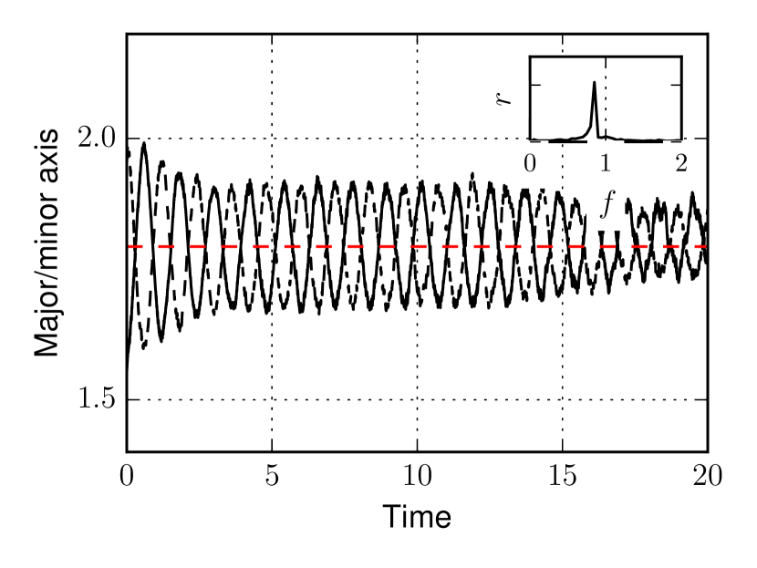
(a) 2D

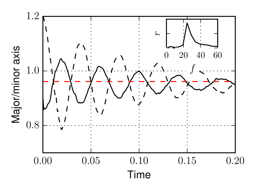
(b) 3D

Figure 1: Time response of radii of an oscillating drop about its reference configuration in 2D and 3D. Insets show the frequency domain of oscillation, showing the frequency of oscillation.

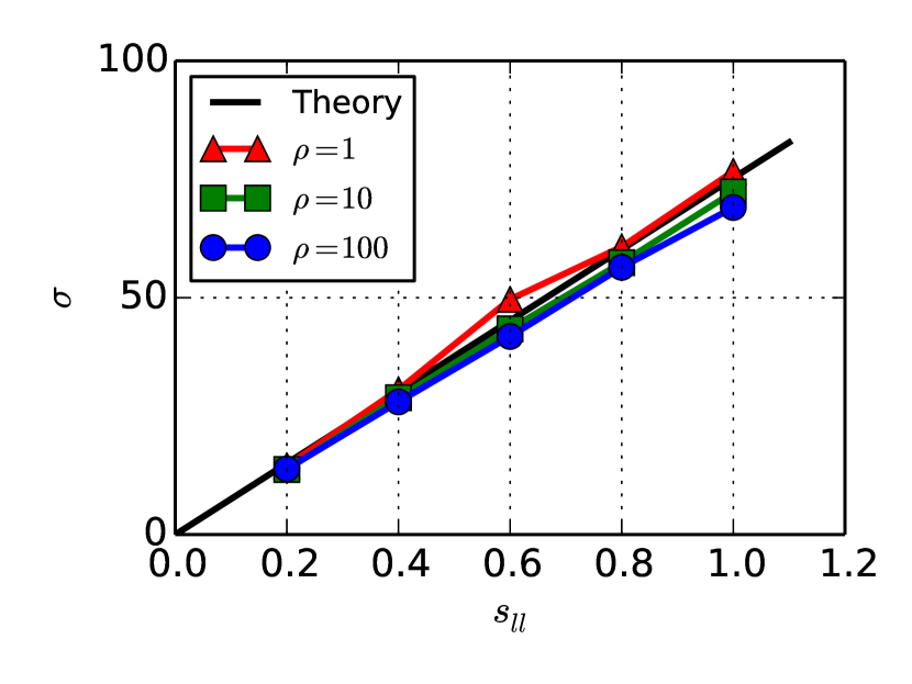
(a) 2D

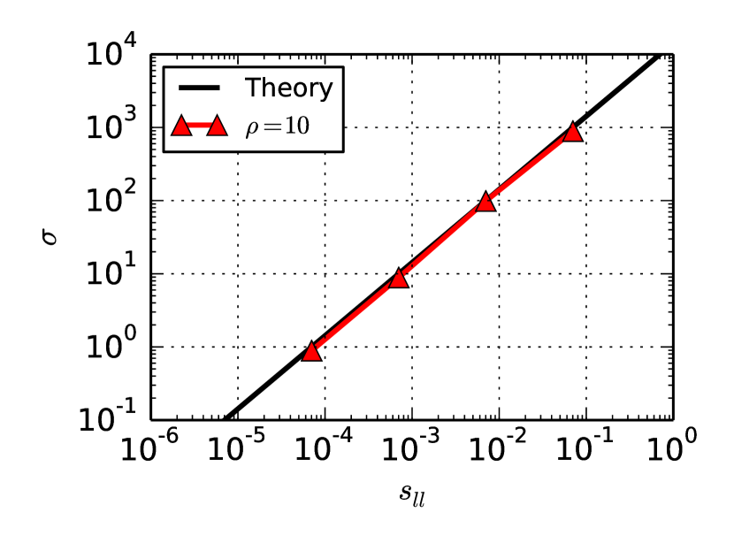
(b) 3D

Figure 2: Linear variation of surface tension coefficient with strength of pairwise potential. The solid black line is obtained from equation 21. For the 2D cases, different densities were considered for the oscillating drop, and potential strengths across orders of magnitude were used in the 3D cases.

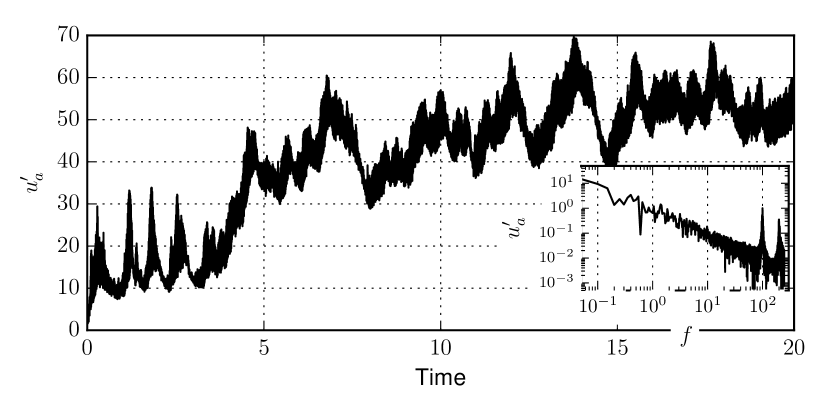
Figure 3: Variation of velocity fluctuation (eq. 29) of a particle with time. Inset shows the presence of high frequency components in the frequency domain of the signal, due to the superimposed inter-particle forces.

The surface tension coefficient for a given particle configuration can be verified by computing the frequency of oscillation of a drop of fluid about its circular (in 2D) or spherical (in 3D) minimal area reference geometry. The time period of oscillation for an inviscid infinite cylindrical jet is given by [28] based on the general results of Rayleigh [32] as:

$$T=2\pi\sqrt{\frac{R^{3}\rho}{6\sigma}}.$$ (27)

For three dimensions, the frequency of shape oscillation (second mode) of a drop is given by:

$$T=\pi\sqrt{\frac{R^{3}\rho}{2\sigma}},$$ (28)

where $T$ is the time period of oscillation, $\rho$ is the density of the liquid, $R$ is the radius of the drop and $\sigma$ is the surface tension coefficient.

Surface tension can thus be measured from these equations by measuring the time period of oscillation of a drop, initially perturbed to an ellipse (or ellipsoid) of equal volume. The time response of the radius of the infinite 2D cylinder and sphere are shown in Fig. 1. The simulation experiment is repeated with liquid drops of different densities and pairwise force strengths for 2D and these results are plotted in Fig. 2(a), and in 3D (Fig. 2(b)) this linear relation is shown to hold good across orders of magnitude of pairwise force strengths. The results show that the relation between potential strength and surface tension is indeed linear, as seen in eq. 23. In these validation cases the smoothing length $h$ is taken to be $3.75$ times the initial particle spacing. A circle of radius $1$ unit is used with a resolution such that the radius is more than $5h$ in these simulations. No viscous model is used in this case.

Though the oscillations are simulated well, the oscillations damp considerably with time, and is more pronounced in the 3D case. This damping is due to the velocity fluctuations in the particles due to the inter particle force model and warrants separate attention. In Fig. 3 we have shown the particle velocity fluctuation for the 2D case, computed by subtracting velocity of each particle from the SPH averaged velocity at that particle position as:

$$u^{\prime}_{a}=\sqrt{\left(u_{ia}-\sum_{b}u_{ib}W_{ab}\frac{m_{b}}{\rho_{b}}\right)^{2}},$$ (29)

where $u_{ia}$ is the velocity component of a particle $a$ in direction $i$, $b$ represent the neighbors of $a$ and the index $i$ is given in Einstein’s summation notation. The inset in the plot shows the frequency domain of the fluctuation. Evidently, there are remarkable peaks in an otherwise power law frequency distribution, at high frequencies. Also, in fig. 1 there is an initial drop in amplitude following which the amplitude remains constant for many oscillations before it deteriorates again. The initial damping could be due to the initial arrangement of particles in an array, which quickly assumes a much lower energy configuration. Further damping is of course due to additional viscosity due to the high frequency oscillations of particles. All this warrants a separate study on the free energy of SPH particles when superimposed by an inter-particle force model. However as we seen here and in the following test cases, the ability of the method to simulate surface tension effects for many practical applications is quite promising.

3.2 Validation of the contact angle model

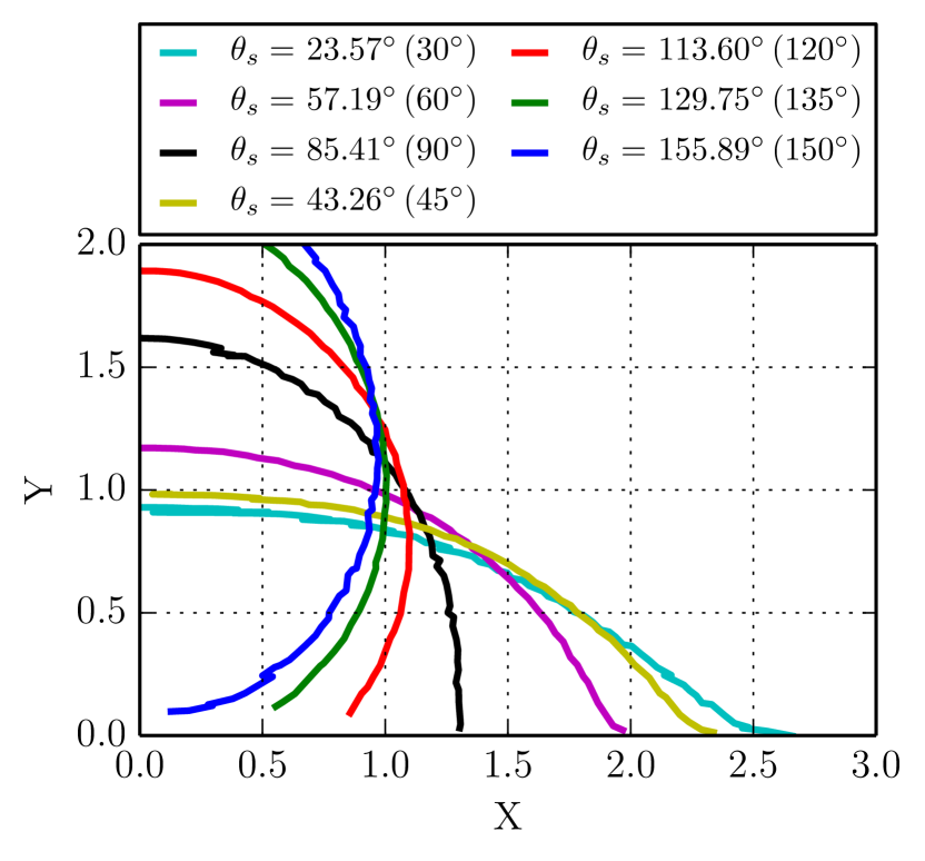
(a) 2D

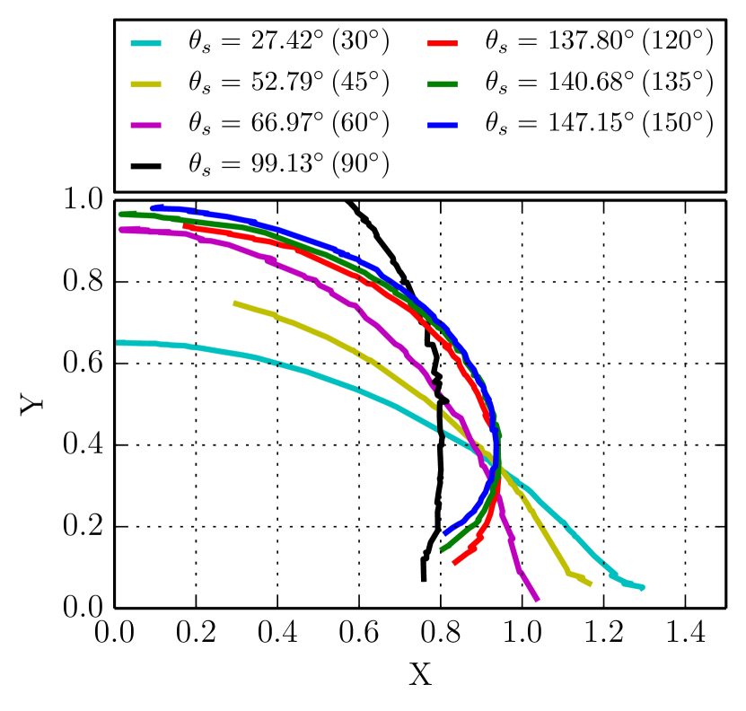
(b) 3D

Figure 4: Contact angles of a sessile drop measured for different potential strength ratios. Values in brackets are the expected angles according to eq. 26

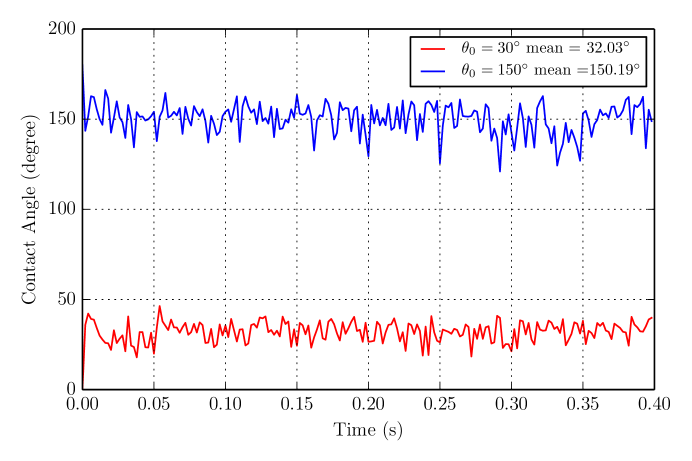
Figure 5: Time variation of the contact angle of a 3D sessile drop for the case of acute ($\theta=30^{\circ}$) and obtuse ($\theta=60^{\circ}$) contact angles. The droplets were initiated from the geometry of hemisphere resting on a solid surface.

The contact angle and incidental wetting behaviour can be controlled in the pairwise force ISPH by varying the relative potential strengths between particles of different phases according to eq. 26. A droplet (in 2D and 3D) initially in a hemispherical configuration (semicircle in 2D) is placed on a solid substrate and is allowed to relax. In the case of obtuse contact angles a gravitational body force was applied on the particle to prevent it from bouncing off. After steady state was reached, a layer of particles lying on the free surface were obtained by a kernel summation criteria and first six particles close to the contact point were chosen and regressed linearly to obtain the apparent contact angle $\theta_{s}$. Figure 4(a) and 4(b) show the profile of the drop for different potential strength pairs. The bracketed values show the expected contact angles computed by eq. 26 in this figure. The resolution and geometry of the drop is similar to the previous validation case for oscillating drops.

In order to demonstrate the evolution of the contact angle with time, we show in fig. 5, the time variation of the contact angle (measured similar to the steady state contact angles) for an obtuse and an acute angle case from the 3D simulations. The plot shows that the angle remains reasonably steady with minor oscillations about its expected value during the relaxation of the drop. This is comparable with pinning a contact angle heuristically applied in case of a traditional mesh based CFD method with a sharp interface model such as the volume of fluids (VOF) method.

3.3 Capillary Rise in 2D

	Height
Width (mm)	Analytical	SPH
0.50	5.01	5.12
0.75	2.78	2.95
1.00	1.56	1.31

Table 1: The capillary rise height for different capillary tube diameters (2D)

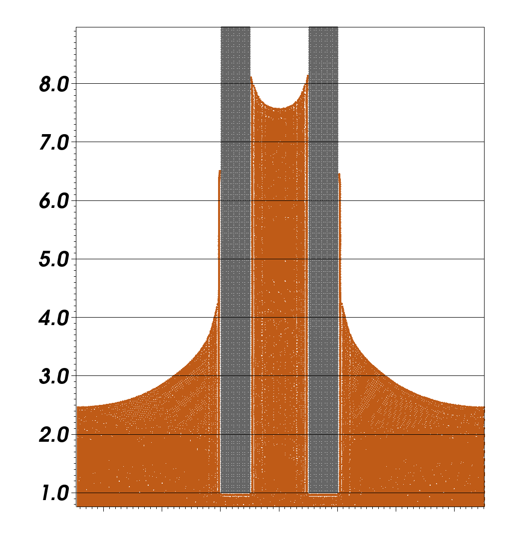
(a) width$=0.5\,mm$

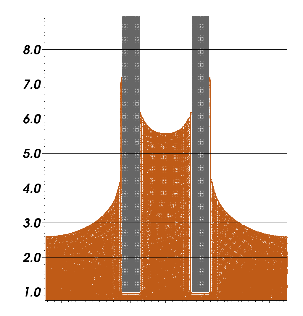
(b) width$=0.75\,mm$

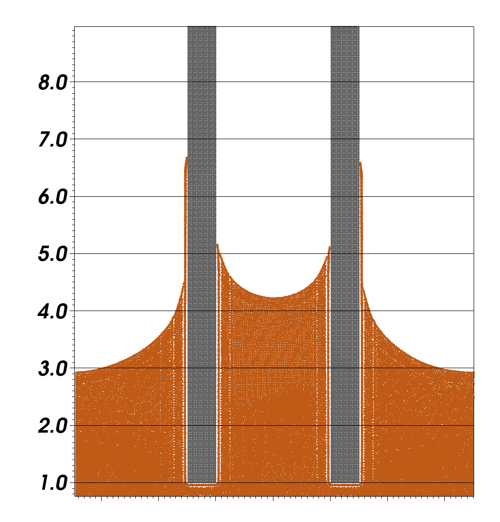
(c) width$=1.0\,mm$

Figure 6: Capillary rise for different tube diameters

Capillary rise of a liquid through a capillary tube is an intricate and useful phenomenon for which analytical solution is straightforward. We construct a simple 2D domain periodic in the horizontal direction with a capillary tube inserted into it. A contact angle of $30^{\circ}$ is chosen in these test case, and is performed for different tube diameters.

The height of capillary liquid column for different capillary diameters can be found in table 1 and the steady state of the simulation for these cases can be seen in fig. 6. The method predicts the rise of the liquid column reasonably accurately, giving confidence for simulations involving surface tension and wetting and their combined effects.

3.4 Drop impact on liquid film

\begin{overpic}[width=433.62pt]{{visit0002.0000}.png} \put(3.0,52.0){\includegraphics[width=390.25534pt]{legend_hot.png}} \end{overpic}

(a) $t=0.2\,ms$

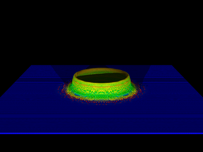
(b) $t=1.7\,ms$

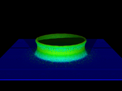
(c) $t=3.45\,ms$

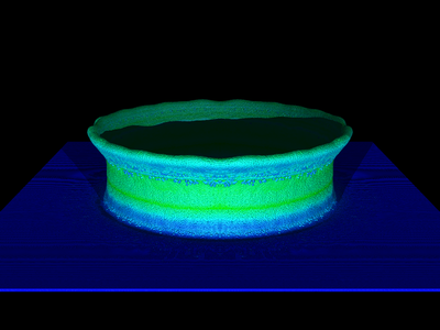
(d) $t=6.2\,ms$

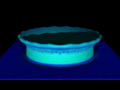
(e) $t=9\,ms$

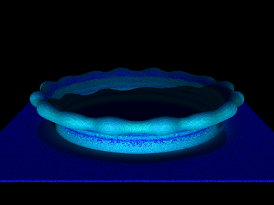
(f) $t=14.9\,ms$

Figure 7: Impact of a droplet on a liquid film with a drop-Weber number, $We_{\textrm{drop}}=273$ and a film-Weber number, $We_{\textrm{film}}=36.5$. The fluid particles are colored by magnitude of velocity, legend on the first image, a.

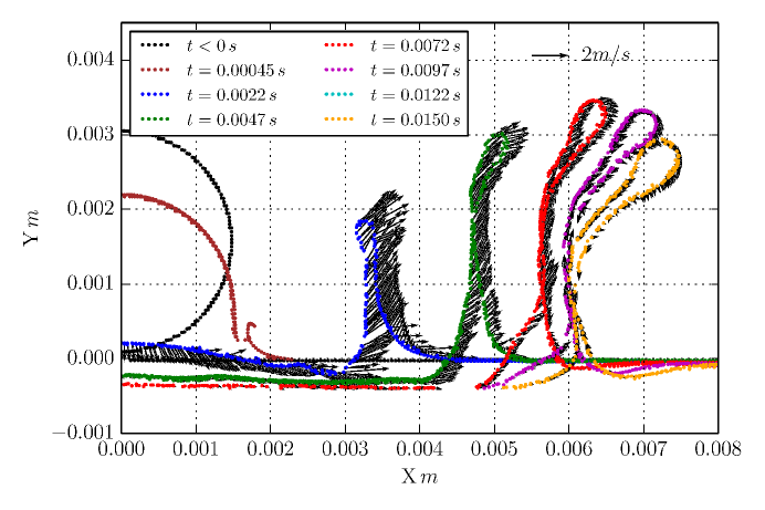
Figure 8: Cross section profile of the splash at different time instances. The grey arrows show the velocity direction of each particle on the surface.

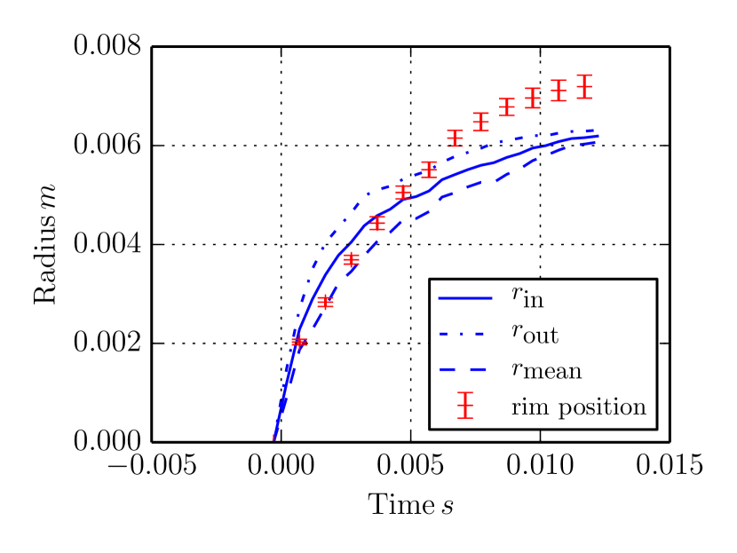
(a) Evolution of crown rim and base

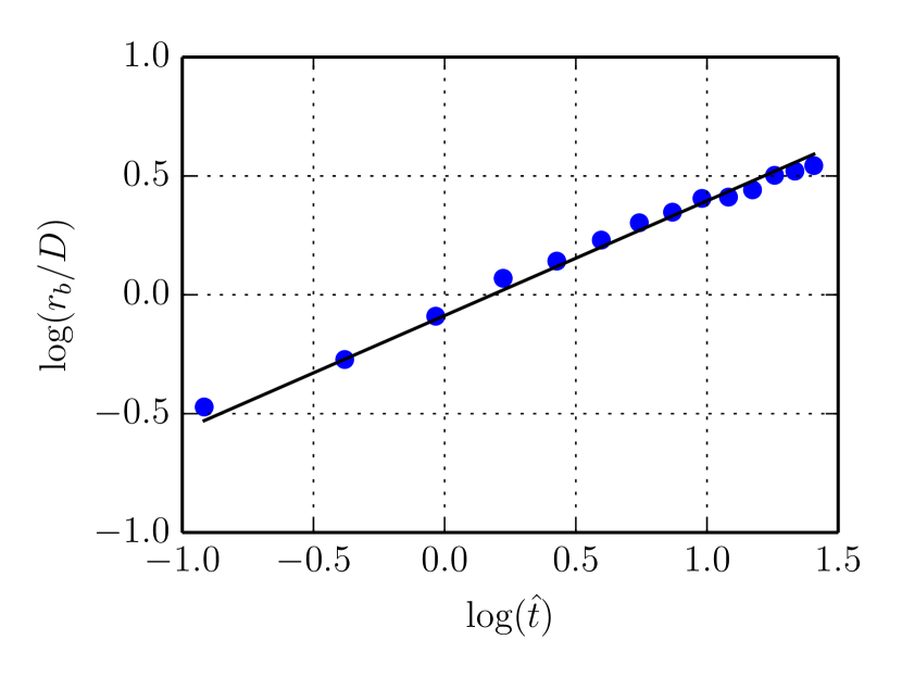
(b) Evolution of base of crown

Figure 9: Time evolution of the splash crown, measured at one vertical plane: $r_{\text{in}}$–inner radius of base of crown, $r_{\text{out}}$–outer radius of base, $r_{\text{mean}}$–mean radius of base of the crown.(a) The center and position of the rim at edge of the crown is shown by red markers to scale. (b) Power law dependence of non-dimensional base radius on non-dimensional time.

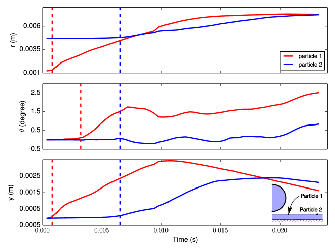
Figure 10: Trajectory of two material points in the liquid film

We simulate the splash of a droplet on a film of the same liquid using the introduced method, after validations. The famous photo of the milk crown by Edgerton and Killian [11] has inspired a number of research works to understand the instability that leads to formation of a crown after a drop of milk impacts a thin liquid film. A thin liquid sheet, ejects immediately from the neck of the impact. Shortly after a uniform splash sheet is formed, surface tension effects begin to dominate and the phenomenon becomes non axisymmetric due to instabilities. The initial part of the splash is driven by mostly inertial effects, and this was studied by axisymmetric simulations [16] and also by free surface SPH simulations [26].

The non dimensional parameters—Weber Number ($We_{drop}=\rho v^{*2}d/\sigma$) and inertia ratio ($\alpha=d/h^{*}$, where $d$ is the diameter of the drop and $h^{*}$ is the thickness of the liquid film)—influence the formation of secondary droplets[18]. The splashing regime encompasses a variety of different morphologies depending on the size and distribution of these droplets [18]. Whether this regime can be explained by a instability mechanism or multiple mechanisms remains an open question [2, 13] today.

We simulate a $3\,mm$ diameter drop splashing on a liquid film impacting at a velocity of $1.8$ m/s on a liquid sheet of height $0.4\,mm$, set as a square trough periodic in both the horizontal directions. The surface tension coefficient for the fluid is set to $0.03505$ N$/$m, corresponding to experiments with milk drops in [18]. This corresponds to a Weber number of $273$. Figure 7 shows the simulation at different time instances, colored by velocity magnitude. In fig. 7d, the onset of an azimuthal undulation is clearly seen. This undulation clearly compares to the splash crown fingers in experiments: 20 crests and troughs are seen in fig. 7 in agreement with the number of sub droplets observed in experiments of milk crown splash (see fig. 2 in [18]) for the corresponding Weber and inertia numbers.

Lattice Boltzmann [22] and DNS [34] simulations have been performed with the imposition of a perturbation of a given wave number or a Gaussian noise, respectively on the liquid film, to trigger the instability. In our simulations no perturbations are imposed, but the noise inherent in SPH method (see fig. 3) triggers the crown forming instability. Splash crown simulations in [5] also make use of ISPH. The undulation on the crown, however, is not discernible from their images, which could be due to the fact that free surface particles were identified to impose the Dirichlet boundary condition. In contrast, the free surface in our simulation is smooth and the features of the splash are discernible.

Figure 8 shows the thickening of the rim of the crown followed by folding of the rim as the expansion of the crown comes to a halt. The arrows indicate the instantaneous velocity of the surface and shows no source of circulation. The temporal evolution of the crown is shown in fig. 9(a). The red markers show the position of the rim of the splash wall over-shooting its base as the base of the splash stops expanding. Figure 9(b) show the non-dimensionalized radius of base of the splash wall having a power law dependence on the non-dimensionalized time. The theoretical results by [46] predict the following power law relation:

$$\frac{r_{b}}{D}=k\hat{t}^{1/2}.$$ (30)

Here, $r_{b}$ is the radius of the splash wall at its base, $D$ is the diameter of the drop, $k$ is a constant that depends on the velocity distribution inside the wall of the splash and $\hat{t}=tV/D$ is the non-dimensional time, where $V$ is the impact velocity of the drop. The slope of line in fig. 9(b) has a value 0.482 which closely corresponds to the square root dependence on time.

The onset of the instability in the splash can be observed as we follow two particles in different location on the initial liquid film as shown in fig. 10. Particle 1 and 2 are chosen as shown in the inset sketch, and are followed as the splash front propagates through them. In the top part of the figure showing radial displacement, both particles are radially displaced by the splash front, as soon as the wave touches them. In the middle of fig. 10, particle 1 is at the azimuthal location ($\theta=0$) for a brief period of time until the instance marked by the red dashed line, after which the particle is azimuthally displaced ($\theta\neq 0$). Particle 2, however is azimuthally displaced right when the splash front reaches it. The vertical displacement also follows trend of the radial displacement. There is therefore a ‘throw’ of the free surface radially and vertically as a wave propagates through it. At some location between the initial positions of particle 1 and 2 the axisymmetry of the wave breaks due to instabilities in the splash crown. This observation is presented to show the advantage a Lagrangian method in tracking instabilities.

4 Dynamic liquid bridge breakage

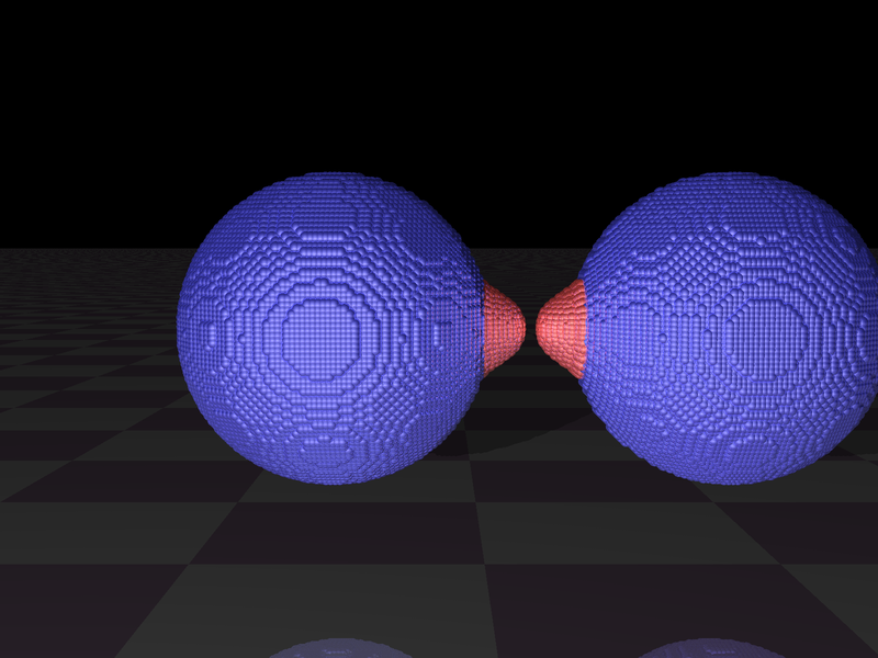
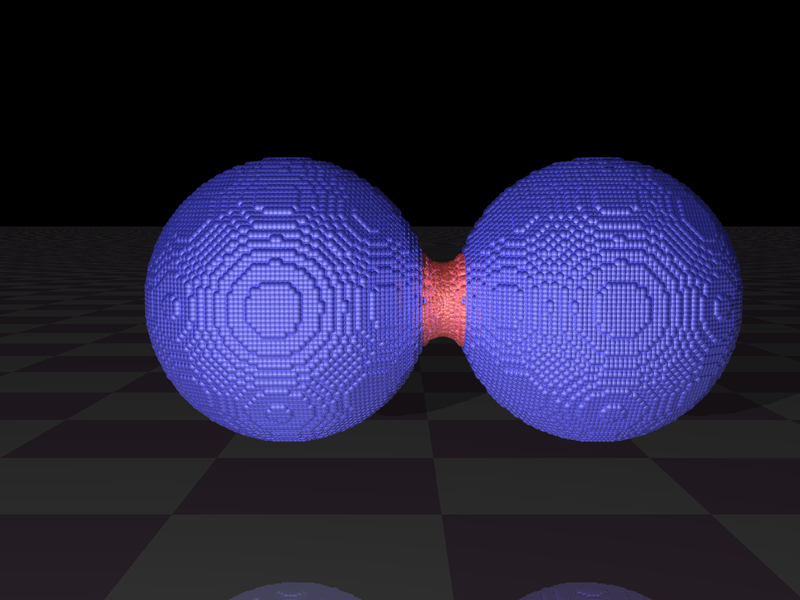
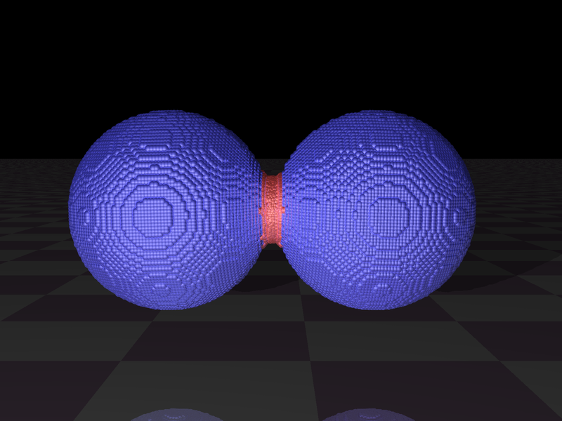
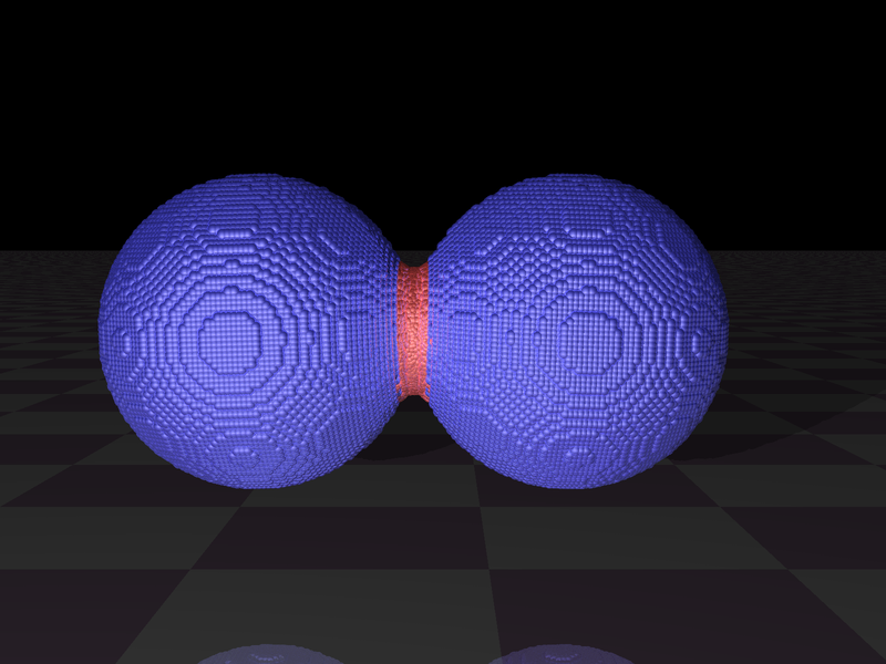
(a) $0.5\,m/s$

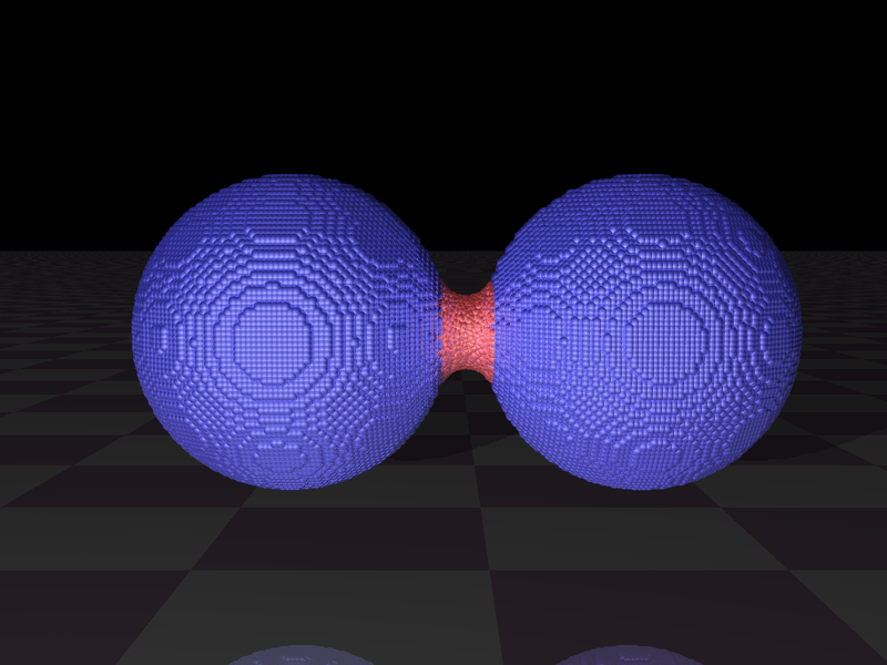
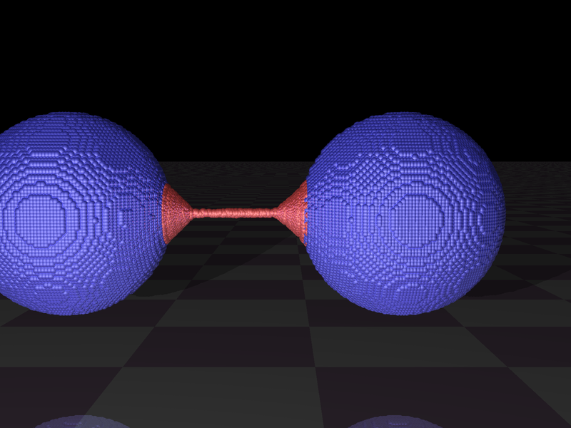
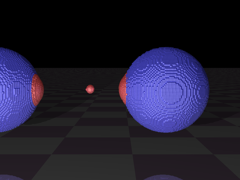
(b) $5\,m/s$

Figure 12: Time instances of collision of two wet solid spheres, for different approach velocities.

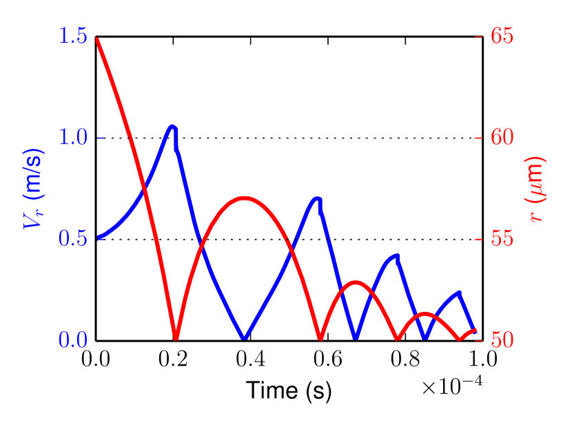
(a) $0.5$ m$/$s

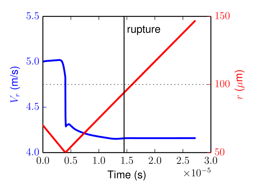
(b) $5$ m$/$s

Figure 13: Relative velocity (left y-axis) and distance (right y-axis) between colliding wet solid spheres for different approach speeds.

In wet granulation processes, agglomeration of granules is a critical step for successful simulations using macroscopic simulation methods such as Discrete Element Method (DEM) [41] or Monte Carlo methods [15]. The analytical criteria used to decide whether capillary bridges will be formed during collision of wet particles for given liquid volume and approach speeds is given by quasi-static considerations. Depending on the dominance of viscous or surface tension effects in the binding liquid, a specific model is used. For example, for viscous dominant binders the following critical velocity for agglomeration is given [12]:

$$v_{c}=\frac{3\pi\mu R_{p}^{2}}{2M_{p}}\left(1+\frac{1}{e}\right)\ln\left(\frac{y}{y_{a}}\right),$$ (31)

where $y$ and $y_{a}$ are the thickness of the liquid layer on the grain and the surface asperity on the grain, respectively. $R_{p}$, $M_{p}$ and $e$ are the radius, mass and restitution coefficient of the grains, respectively. Other class of analytical models assume a surface tension dominance to compute the force between the grains for different static configurations of the liquid bridge, for example a pendular shape [30]. In reality, the bridge deforms quite rapidly and inertial forces compete with surface tension forces deforming the interface non-linearly and a general analytical solution to the problem is difficult.

We performed a range of simulations of colliding wet spheres to find the critical velocity at which the particles stop agglomerating. This is compared to results from the purely viscous analytical model given in eq.31 and a numerical result using a grid based method [17]. Two solid spheres of diameter 50 $\mu$m are considered, with a fluid drop of total volume $1072\,\mu$m³ divided into two drops and placed as sessile drops on both the spheres. The viscosity and surface tension of the liquid are 0.001 Nsm^-2 and 0.071 N/m respectively. These simulation parameters are similar to those used in [17] for a similar study of dynamic liquid bridges. One of the particles is launched at the other; upon contact of the liquid surfaces the drops coalesce and a liquid bridge is formed. The collision between the rigid solid spheres is assumed to be purely elastic (restitution coefficient, $e=1$) and takes place at a point immersed within the liquid bridge.

In figure 12, liquid bridge configuration at different time instances for two different approach velocities are shown. The rupture of liquid bridge following collision of the solid spheres is shown in fig. 12(b) for an approach velocity of $5$ m$/$s, which is beyond the critical value for agglomeration. The liquid bridge thins to form a near cylindrical filament before rupture. The filament then breaks and relaxes to a satellite drop. In fig. 12(a), on the other hand, the liquid bridge sustains itself and causes agglomeration of the solids. In figure 13 the distance between the two solid spheres and relative velocity are shown as a function of times. For the smaller velocity considered (fig. 13(a)), the bridge sustains and results in the particles bouncing off of each other repeatedly while remaining agglomerated. For velocity larger than critical value (fig. 13(b)), the bridge ruptures and particles depart at constant velocities following rupture. A series of simulations were performed and a value of 1.1 m$/$s is found to be the critical velocity for agglomeration of the solid spheres. This value is about an order of magnitude higher than that predicted by the analytical model given by eq. 31: a value of 0.16 m$/$s. In a similar study using a constrained interpolation method with a VOF model for interface predicted a critical velocity of 2.6 m/s [17]. The reason for this discrepancy should depend on the resolution of the interface near the rupture and requires verification with experiments yet to be published. However a clear underprediction of critical velocity by a widely used analytical model is evident. With a series of numerical experiments very accurate models for the micromechanics of collision/agglomeration can therefore be developed for different regimes of viscous and surface tension forces, using the introduced ISPH method.

5 Conclusion

Incompressible Smoothed Particle Hydrodynamics (ISPH), a more accurate and robust variant of the SPH method is improved in scope to include freesurface surface tension and wetting problems. The competence of this improved meshless method in studying complex flows encountered at small scales is demonstrated through three dimensional simulations of dynamic capillary phenomena. The unexplained artificial viscosity due to inter particle forces needs further analysis.

References

- Adami et al. [2010] Adami, S., Hu, X., Adams, N., 2010. A new surface-tension formulation for multi-phase sph using a reproducing divergence approximation. J. Comput. Phys. 229 (13), 5011–5021.
- Agbaglah and Deegan [2014] Agbaglah, G., Deegan, R., 2014. Growth and instability of the liquid rim in the crown splash regime. J. Fluid Mech. 752, 485–496.
- Akinci et al. [2013] Akinci, N., Akinci, G., Teschner, M., 2013. Versatile surface tension and adhesion for sph fluids. ACM Trans. Graphics 32 (6), 182.
- Allen and Tildesley [1989] Allen, M. P., Tildesley, D. J., 1989. Computer simulation of liquids. Oxford university press.
- Aly et al. [2013] Aly, A. M., Asai, M., Sonda, Y., 2013. Modelling of surface tension force for free surface flows in isph method. Int. J. Numer. Methods Heat Fluid Flow 23 (3), 479–498.
- Brackbill et al. [1992] Brackbill, J., Kothe, D. B., Zemach, C., 1992. A continuum method for modeling surface tension. J. Comput. Phys. 100 (2), 335–354.
- Colagrossi and Landrini [2003] Colagrossi, A., Landrini, M., 2003. Numerical simulation of interfacial flows by smoothed particle hydrodynamics. J. Comput. Phys. 191 (2), 448–475.
- Colagrossi et al. [2013] Colagrossi, A., Souto-Iglesias, A., Antuono, M., Marrone, S., 2013. Smoothed-particle-hydrodynamics modeling of dissipation mechanisms in gravity waves. Phys. Rev. E 87 (2), 023302.
- Dehnen and Aly [2012] Dehnen, W., Aly, H., 2012. Improving convergence in smoothed particle hydrodynamics simulations without pairing instability. Mon. Not. R. Astron. Soc. 425 (2), 1068–1082.
- DussanV [1976] DussanV, E., 1976. Moving contact line-slip boundary-condition. J. Fluid Mech. 77 (OCT 22), 665–684.
- Edgerton and Killian [1954] Edgerton, H. E., Killian, J. R., 1954. Flash!: Seeing the unseen by ultra high-speed photography. CT Branford Co.
- Ennis et al. [1991] Ennis, B. J., Tardos, G., Pfeffer, R., 1991. A microlevel-based characterization of granulation phenomena. Powder Technol. 65 (1-3), 257–272.
- Fullana and Zaleski [1999] Fullana, J. M., Zaleski, S., 1999. Stability of a growing end rim in a liquid sheet of uniform thickness. Phys. Fluids (1994-present) 11 (5), 952–954.
- Hirt and Nichols [1981] Hirt, C. W., Nichols, B. D., 1981. Volume of fluid (vof) method for the dynamics of free boundaries. J. Comput. Phys. 39 (1), 201–225.
- Hussain et al. [2013] Hussain, M., Kumar, J., Peglow, M., Tsotsas, E., 2013. Modeling spray fluidized bed aggregation kinetics on the basis of monte-carlo simulation results. Chem. Eng. Sci. 101, 35–45.
- Josserand and Zaleski [2003] Josserand, C., Zaleski, S., 2003. Droplet splashing on a thin liquid film. Phys. Fluids 15 (6), 1650–1657.
- Kan et al. [2015] Kan, H., Nakamura, H., Watano, S., 2015. Numerical simulation of particle–particle adhesion by dynamic liquid bridge. Chem. Eng. Sci. 138, 607–615.
- Krechetnikov and Homsy [2009] Krechetnikov, R., Homsy, G. M., 2009. Crown-forming instability phenomena in the drop splash problem. J. Colloid Interface Sci. 331 (2), 555–559.
- Lee et al. [2008] Lee, E.-S., Moulinec, C., Xu, R., Violeau, D., Laurence, D., Stansby, P., 2008. Comparisons of weakly compressible and truly incompressible algorithms for the sph mesh free particle method. J. Comput. Phys. 227 (18), 8417–8436.
- Liu and Liu [2010] Liu, M., Liu, G., 2010. Smoothed particle hydrodynamics (sph): an overview and recent developments. Arch. Comput. Methods Eng. 17 (1), 25–76.
- Mikami et al. [1998] Mikami, T., Kamiya, H., Horio, M., 1998. Numerical simulation of cohesive powder behavior in a fluidized bed. Chem. Eng. Sci. 53 (10), 1927–1940.
- Ming and Jing [2014] Ming, C., Jing, L., 2014. Lattice boltzmann simulation of a drop impact on a moving wall with a liquid film. Comput. Math. Appl. 67 (2), 307–317.
- Monaghan [1994] Monaghan, J. J., 1994. Simulating free surface flows with sph. J. Comput. Phys. 110 (2), 399–406.
- Morris [2000] Morris, J. P., 2000. Simulating surface tension with smoothed particle hydrodynamics. Int. J. Numer. Methods Fluids 33 (3), 333–353.
- Morris et al. [1997] Morris, J. P., Fox, P. J., Zhu, Y., 1997. Modeling low reynolds number incompressible flows using sph. J. Comput. Phys. 136 (1), 214–226.
- Nair and Tomar [2014] Nair, P., Tomar, G., 2014. An improved free surface modeling for incompressible sph. Comput. Fluids 102, 304–314.
- Nair and Tomar [2017] Nair, P., Tomar, G., 2017. A study of energy transfer during water entry of solids using incompressible sph simulations. Sādhanā 42 (4), 517–531.
- Nugent and Posch [2000] Nugent, S., Posch, H., 2000. Liquid drops and surface tension with smoothed particle applied mechanics. Phys. Rev. E 62 (4), 4968.
- Peskin [2002] Peskin, C. S., 2002. The immersed boundary method. Acta Numerica 11, 479–517.
- Pitois et al. [2001] Pitois, O., Moucheront, P., Chateau, X., 2001. Rupture energy of a pendular liquid bridge. Eur. Phys. J. B 23 (1), 79–86.
- Popinet [2009] Popinet, S., 2009. An accurate adaptive solver for surface-tension-driven interfacial flows. J. Comput. Phys. 228 (16), 5838–5866.
- Rayleigh [1879] Rayleigh, L., 1879. On the capillary phenomena of jets. Proc. R. Soc. Lond. 1 29 (196-199), 71–97.
- Renardy et al. [2001] Renardy, M., Renardy, Y., Li, J., 2001. Numerical simulation of moving contact line problems using a volume-of-fluid method. J. Comput. Phys. 171 (1), 243–263.
- Rieber and Frohn [1999] Rieber, M., Frohn, A., 1999. A numerical study on the mechanism of splashing. Int. J. Numer. Methods Heat Fluid Flow 20 (5), 455–461.
- Rowlinson and Widom [2013] Rowlinson, J. S., Widom, B., 2013. Molecular theory of capillarity. Courier Corporation.
- Szewc et al. [2012] Szewc, K., Pozorski, J., Minier, J.-P., 2012. Analysis of the incompressibility constraint in the smoothed particle hydrodynamics method. Int. J. Numer. Methods Eng. 92 (4), 343–369.
- Tartakovsky and Meakin [2005] Tartakovsky, A., Meakin, P., 2005. Modeling of surface tension and contact angles with smoothed particle hydrodynamics. Phys. Rev. E 72 (2), 026301.
- Tartakovsky and Meakin [2006] Tartakovsky, A. M., Meakin, P., 2006. Pore scale modeling of immiscible and miscible fluid flows using smoothed particle hydrodynamics. Adv. Water Resour. 29 (10), 1464–1478.
- Tartakovsky and Panchenko [2016] Tartakovsky, A. M., Panchenko, A., 2016. Pairwise force smoothed particle hydrodynamics model for multiphase flow: surface tension and contact line dynamics. J. Comput. Phys. 305, 1119–1146.
- Tomar et al. [2005] Tomar, G., Biswas, G., Sharma, A., Agrawal, A., 2005. Numerical simulation of bubble growth in film boiling using a coupled level-set and volume-of-fluid method. Phys. Fluids 17 (11), 112103.
- Tsunazawa et al. [2016] Tsunazawa, Y., Fujihashi, D., Fukui, S., Sakai, M., Tokoro, C., 2016. Contact force model including the liquid-bridge force for wet-particle simulation using the discrete element method. Adv. Powder Technol. 27 (2), 652–660.
- Violeau [2012] Violeau, D., 2012. Fluid Mechanics and the SPH method: theory and applications. Oxford University Press.
- Violeau and Rogers [2016] Violeau, D., Rogers, B. D., 2016. Smoothed particle hydrodynamics (sph) for free-surface flows: past, present and future. J. Hydraul. Res. 54 (1), 1–26.
- Wendland [1995] Wendland, H., 1995. Piecewise polynomial, positive definite and compactly supported radial functions of minimal degree. Adv. Comput. Math 4 (1), 389–396.
- Yabe et al. [2001] Yabe, T., Xiao, F., Utsumi, T., 2001. The constrained interpolation profile method for multiphase analysis. J. Comput. Phys. 169 (2), 556–593.
- Yarin and Weiss [1995] Yarin, A., Weiss, D., 1995. Impact of drops on solid surfaces: self-similar capillary waves, and splashing as a new type of kinematic discontinuity. J. Fluid Mech. 283, 141–173.
- Ye et al. [2005] Ye, Q., Domnick, J., Scheibe, A., Pulli, K., 2005. Numerical simulation of electrostatic spray-painting processes in the automotive industry. In: High Performance Computing in Science and Engineering’04. Springer, pp. 261–275.
- Zhang [2010] Zhang, M., 2010. Simulation of surface tension in 2d and 3d with smoothed particle hydrodynamics method. J. Comput. Phys. 229 (19), 7238–7259.