Lattice symmetries, spectral topology and opto-electronic properties of graphene-like materials

Abstract

The topology of the band structure, which is determined by the lattice symmetries, has a strong influence on the transport properties. Here we consider an anisotropic honeycomb lattice and study the effect of a continuously deformed band structure on the optical conductivity and on diffusion due to quantum fluctuations. In contrast to the behavior at an isotropic node we find super- and subdiffusion for the anisotropic node. The spectral saddle points create van Hove singularities in the optical conductivity, which could be used to characterize the spectral properties experimentally.

I Introduction

Graphene, a two-dimensional sheet of carbon atoms which form a honeycomb lattice has exceptional opto-electronic properties novoselov05 . The latter are related to the bandstructure of this material, consisting of two bands with two Dirac nodes castro09 ; abergel10 . The existence and the positions of these nodes are a consequence of global symmetries of the lattice. Local breaking of the symmetries, for instance, by impurities or other types of local disorder does not affect the robust opto-electronic properties, as long as the symmetries are globally preserved. This is the case when the distribution of the local disorder obeys the global symmetries. The situation changes, though, when the symmetries are globally broken. A typical example is breaking of the sublattice symmetry of the honeycomb lattice when the carbon atoms are replaced by atoms with different mass, such that the atomic mass is larger on one sublattice. This leads to an opening of the Dirac nodes by creating a gap between the two bands. A realization of this effect is hexagonal Boron Nitride, which is characterized by a gap of 5 eV watanabe04 . Another global symmetry of the honeycomb lattice is its isotropy. Breaking this symmetry by changing the bonds between neighboring sites of the atomic lattice in one direction affects the positions of the Dirac nodes. For special values of the anisotropic bonds the Dirac nodes can even brought to the the same position with only one degenerate node between the two bands. This effect was proposed and discussed in a series of papers by Montambaux et al. montambaux09 ; montambaux09a ; delplace10 ; adroguer16 , and as a Lifshitz transition it was also discussed recently in the context of the Kitaev model faye14 . In particular, the spectral properties and the DC conductivity become very anisotropic in the case of the doubly degenerate Dirac node adroguer16 . This is quite remarkable in the light of transport properties in graphene-like materials, which are already exceptional near the Dirac nodes in isotropic graphene. We briefly summarize the DC transport properties in undoped isotropic graphene.

Diffusion, the origin of conducting behavior in conventional metals with finite conductivity, is a result of random impurity scattering thouless74 . In the absence of the latter the diffusion coefficient would diverge and we would experience ballistic transport. This simple picture is not valid at spectral degeneracies, though. For instance, at a Dirac (Weyl) node or at a node with parabolic spectrum there is diffusion due to quantum fluctuations between the upper and the lower band, even in the absence of random impurity scattering (cf. Appendix B). In this context it should be noted that the Fermi Golden Rule gives adroguer16

$$\sigma_{\mu\mu}=\frac{e^{2}\hbar}{\pi\gamma}v_{F}^{2}\ ,$$ (1)

where $\gamma$ is the strength of the disorder fluctuations and $v_{F}$ is the Fermi velocity. It does not reproduce the constant conductivity at the node in the pure limit $\gamma\to 0$

$$\sigma_{\mu\mu}=\frac{e^{2}}{\pi h}\ ,$$ (2)

which was experimentally confirmed for graphene novoselov05 ; chen08 ; chen09 (up to the factor $1/\pi$). The finiteness of the conductivity at the node of the pure system can be attributed to quantum fluctuations between the two bands. The latter are not taken into account in the Fermi Golden Rule (1), whereas their inclusion leads to a finite conductivity at the Dirac node even in the absence of any impurity scattering. This result reflects a more delicate transport behavior at the spectral node, whereas away from this node conventional approximations, such as Fermi Golden Rule (1), are valid.

The result (2) of an isotropic nodal spectrum is in stark contrast to the recently found behavior for an anisotropic spectrum in the vicinity of a Dirac node. Adroguer et al. adroguer16 found a remarkable result for the conductivity in the presence of random scattering, namely a strongly anisotropic transport behavior, where $\sigma_{xx}(E_{F})$ vanishes linearly with $E_{F}\to 0$, whereas $\sigma_{yy}(E_{F})$ stays nonzero even for $E_{F}\to 0$. We will return to the details of this result in Sect. II.

The paper is organized as follows. In Sect. II the tight-binding model of an anisotropic honeycomb lattice is briefly considered, including its relation to a Dirac-like low-energy Hamiltonian. For this Hamiltonian the optical conductivities (Sect. III) and the diffusion coefficients (Sect. IV) are calculated. These results and their relations to topological transitions are discussed in Sect. V.

Figure 1: A hexagon of the honeycomb lattice with hopping parameters $t_{1}$, $t_{2}$ and $t_{3}$. The thickness of the bonds refer to the hopping rate. Full (empty) circles indicate the two triangular sublattices.

II Model of merging Dirac nodes

The Hamiltonian of a tight-binding model with honeycomb structure (e.g., graphene) reads in sublattice representation of the two-dimensional ${\bf k}$ space castro09 ; abergel10

$$H=\pmatrix{0&-\sum_{j=1}^{3}t_{j}e^{i{\bf a}_{j}\cdot{\bf k}}\cr-\sum_{j=1}^{3}t_{j}e^{-i{\bf a}_{j}\cdot{\bf k}}&0\cr}$$ (3)

with the basis vector of the sublattice with empty circles in Fig. 1

$${\bf a}_{1}=a(0,-1),\ \ {\bf a}_{2,3}=\frac{a}{2}(\pm\sqrt{3},1)$$ (4)

and with the lattice constant $a$ of this sublattice. For fixed basis vectors ${\bf a}_{j}$ the positions of the two Dirac nodes depend on the hopping parameters $t_{1,2,3}$. Increasing one of them relative to the others (i.e., breaking isotropy) moves the Dirac nodes towards each other. This is accompanied by lifting the degenerate saddle points of the spectrum. In particular, the Dirac nodes merge if two tunneling parameters are equal and the third one is twice as large, for instance, for $t_{1}=2t_{2}=2t_{3}$ (cf. Fig. 3). For simplicity, we consider subsequently only $t_{2}=t_{3}\equiv t$.

Figure 2: Band structure of the honeycomb lattice for $t_{1}=2t$ (top) and $t_{1}=3t$ (bottom).

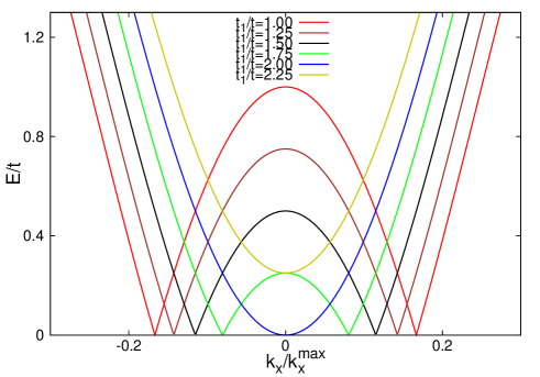
Figure 3: Merging of two Dirac nodes with increasing anisotropy. For $t_{1}=2.25t$ there is a gap.

At this point the Hamiltonian reads in the vicinity of the merged Dirac nodes

$$H=\frac{p_{x}^{2}}{2m}\sigma_{x}+c_{y}p_{y}\sigma_{y}\ ,$$ (5)

where $\sigma_{j}$ are Pauli matrices with the $2\times 2$ unit matrix $\sigma_{0}$ with coefficients $m$ and $c_{y}$, which are related to the tunneling rates $t_{j}$ in a rather complex manner montambaux09 . Thus, the tuning of $t_{1}$ allows us to measure the effect of the internode scattering on the transport properties.

Adroguer et al. adroguer16 found with the Hamiltonian (5) for the conductivity in the presence of a random scattering rate $\gamma$

$$\sigma_{xx}(E_{F})\approx 0.197\ \frac{e^{2}\hbar}{\pi\gamma}\frac{2E_{F}}{m}\ ,\ \ \ \sigma_{yy}(E_{F})\approx 1.491\ \frac{e^{2}\hbar}{\pi\gamma}c_{y}^{2}\ .$$ (6)

The conductivity $\sigma_{yy}(E_{F})$ diverges for vanishing disorder, while the behavior of $\sigma_{xx}(E_{F})$ diverges with $\gamma\sim 0$ only for $E_{F}\neq 0$. On the other hand, the result is not unique in the limit $E_{F}\to 0$, $\gamma\to 0$.

Since the conductivity is proportional to the diffusion coefficient of scattered electrons at the Fermi energy $E_{F}$ due to the Einstein relation, the result in Eq. (6) reflects also a strongly anisotropic diffusion coefficient at the anisotropic Dirac node with $E_{F}=0$. This shall be studied in this paper in the absence of random scattering. For potential opto-electronic applications it is important to analyze the optical conductivity.

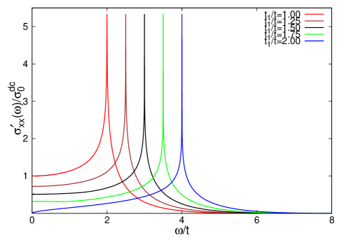
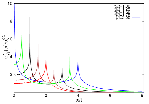
Figure 4: Optical conductivities $\sigma_{xx}^{\prime}$ and $\sigma_{yy}^{\prime}$ with moving van Hove singularities for different strengths of the anisotropy. The van Hove singularity for $\sigma_{yy}^{\prime}$ of the isotropic system is split by the anisotropy into a pair of van Hove singularities, which move apart with increasing anisotropy.

III Optical conductivity

The linear response of the electronic system to an electromagnetic field of frequency $\omega$ is described by the Kubo formula of the optical conductivity. At temperature $T$ this reads

$$\sigma_{\mu\nu}(\omega)=-\frac{i}{\hbar}\lim_{\alpha\to 0}\int_{BZ}\sum_{l,l^{\prime}=0,1}\frac{\langle k,l|j_{\mu}|k,l^{\prime}\rangle\langle k,l^{\prime}|j_{\nu}|k,l\rangle}{E_{k,l}-E_{k,l^{\prime}}+\omega-i\alpha}\frac{f_{\beta}(E_{k,l^{\prime}})-f_{\beta}(E_{k,l})}{E_{k,l}-E_{k,l^{\prime}}}\frac{d^{2}k}{\Omega_{BZ}}$$ (7)

with the Fermi-Dirac distribution $f_{\beta}(E)=1/[1+\exp(\beta(E-E_{F}))]$, $\beta=1/k_{b}T$. $\Omega_{BZ}$ is the area of the Brillouin zone $BZ$, and $l,l^{\prime}$ refers to the band index. Its derivation can be found, for instance, in Ref. hill11 . This formula gives us for the Hamiltonian (5) with $T\sim 0$, $E_{F}=0$ and $\omega>0$

$$Re[\sigma_{xx}(\omega)]\equiv\sigma_{xx}^{\prime}\sim\omega^{1/2}I_{x}\ ,\ \ \ Re[\sigma_{yy}(\omega)]\equiv\sigma_{yy}^{\prime}\sim\omega^{-1/2}I_{y}$$ (8)

for small $\omega$, where $I_{x,y}$ are $\omega$-independent integrals. Thus, the anisotropy of the optical conductivity depends strongly on $\omega$. The corresponding optical conductivity of an isotropic Dirac node is independent of $\omega$. For the full Hamiltonian (3) and arbitrary values of $\omega$ the behavior of $\sigma_{xx}^{\prime}$ and $\sigma_{yy}^{\prime}$ is plotted in Figs. 4 – 5. For higher frequencies the behavior of the two conductivities is compared in Fig. 5.

The real part of the integrand in Eq. (7) contains a Dirac Delta function for $\alpha\sim 0$, which picks $E_{k,l^{\prime}}-E_{k,l}=\omega$. Thus $\sigma_{\mu\mu}^{\prime}=0$ for $\omega$ smaller than the gap hill11 .

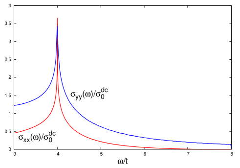
Figure 5: High-frequency behavior of $\sigma_{xx}^{\prime}$ and $\sigma_{yy}^{\prime}$ near the van Hove singularity at $\omega=4t$ of the anisotropic lattice with $t_{1}=2t$, where the effect of the anisotropy is weak.

IV Anomalous diffusion

The motion of particles (e.g., electrons) is characterized by the mean square displacement of a particle position, a concept which has been applied to classical as well as to quantum systems thouless74 . It provides our basic understanding for a large number of transport phenomena, such as the metallic behavior in electronic systems. Starting point is the transition probability for a particle, governed by the Hamiltonian $H$, to move from the site ${\bf r}^{\prime}$ on a lattice to another lattice site ${\bf r}$ within the time $t$:

$$P_{{\bf r}{\bf r}^{\prime}}(t)=\sum_{j,j^{\prime}}|\langle{\bf r},j|e^{-iHt}|{\bf r}^{\prime},j^{\prime}\rangle|^{2}\ .$$ (9)

Here the indices $j,j^{\prime}$ refer to different bands of the system, represented in the Hamiltonian (3) or (5) by Pauli matrices. With the expression (9) we obtain, for instance, the mean square displacement as

$$\langle(r_{\mu}-r^{\prime}_{\mu})^{2}\rangle=\sum_{r}(r_{\mu}-r_{\mu}^{\prime})^{2}P_{{\bf r}{\bf r}^{\prime}}(t)\ \ \ (\mu=x,y)\ .$$

After integration with respect to time this becomes according to Eq. (13)

$$\varepsilon^{2}\sum_{\bf r}(r_{\mu}-r_{\mu}^{\prime})^{2}\int_{0}^{\infty}P_{{\bf r}{\bf r}^{\prime}}(t)e^{-\varepsilon t}dt=\int D_{\mu}(\varepsilon,E)dE$$ (10)

with $D_{\mu}(\varepsilon,E)$ defined in Eq . (17). Thus, we obtain the integral of the diffusion coefficient $D_{\mu}(\varepsilon,E)$ for a particle of energy $E$ with respect to all energies. In the case of a Fermi gas only fermions at the Fermi energy contribute at sufficiently low temperatures. Therefore, we study this coefficient for particles at a fixed Fermi energy $E$. Next, $D_{\mu}(\varepsilon,E)$ is calculated for a node with linear and/or parabolic spectrum, as given for the merging point of two Dirac nodes in Eq. (5). With the expression (18) for the diffusion coefficient we obtain from Eqs. (24) and (25)

$$D_{x}\approx{\bar{D}}_{x}\varepsilon^{1/2}\ ,\ \ \ D_{y}\approx{\bar{D}}_{y}\varepsilon^{-1/2}\ ,$$ (11)

where the $\varepsilon$–independent coefficients ${\bar{D}}_{x}$ and ${\bar{D}}_{y}$ are integrals given in App. C.

These expressions for the diffusion coefficients reflect the result of a divergent $\sigma_{yy}$ for $\gamma\to 0$ in Eq. (6) and clarifies the transport behavior at $E_{F}=0$ and $\gamma=0$, previously found in Ref. adroguer16 . It corresponds with the asymptotic time ($\tau$) behavior of superdiffusion ($\sim\tau^{3/2}$) in $y$ direction and subdiffusion (i.e., $\sim\tau^{1/2}$) in $x$ direction. For an isotropic node we get $D^{(1)}\sim 4\pi/3$ for a linear (Dirac) dispersion and $D^{(2)}\sim 8\pi/3$ for quadratic dispersion, respectively (cf. App. B).

We anticipate that additional disorder scattering would replace $\varepsilon$ by disorder strength $\gamma$ which reduces the superdiffusive behavior to normal diffusion in the $y$ direction, whereas the subdiffusive behavior in the $x$ direction would persist. This agrees with the behavior of the conductivity in Eq. (6).

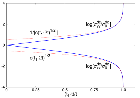
Figure 6: Scaling behavior of the conductivity for $\omega\sim 0$ with the strength of the anisotropy.

V Discussion

Transport properties are very sensitive to the topology of the band structure. We have studied this in terms of the optical conductivity and mean-square displacement for a system, where the topology of the band structure is characterized by two bands with two nodes and saddle points between these nodes (i.e., a vanishing gradient of the spectrum $\nabla_{\bf k}E_{\bf k}=0$ with different curvatures in different directions). For our study it is essential that in real space we have a lattice with global symmetries. For instance, there is a sublattice symmetry due to the two degenerate triangular lattices forming a honeycomb lattice and a discrete threefold isotropy. Then the band structure of the infinite lattice is a continuous compact manifold. Continuous deformations of the latter can be achieved by breaking global lattice symmetries. For example, breaking the sublattice symmetry opens the Dirac nodes and creates a gap between the two bands castro09 ; abergel10 . The size of the gap increases continuously with increasing sublattice asymmetry. Breaking the global isotropy of the lattice by changing the electronic hopping rate in one direction, breaks the isotropy of the nodal structure and moves the nodes to different locations in ${\bf k}$ space montambaux09 ; montambaux09a ; delplace10 ; adroguer16 . At the same time the degeneracy of the saddle points is lifted. The reduction of the saddle point value upon an increasing anisotropy is visualized in Fig. 3.

Spectral properties are difficult to observe directly; it is easier to analyze them indirectly through transport measurements. For instance, the saddle points in the spectrum lead to van Hove singularities in the optical conductivity (cf. Figs. 4 and 5). Nodes, on the other hand, are characterized by a kind of universal transport behavior when random scattering is suppressed, as discussed in Sect. I. This limit reveals details of the spectrum at the nodes. More directly, though, is the measurement of the optical conductivity for low frequencies.

The main effect of a globally broken isotropy on the optical conductivity $\sigma_{yy}^{\prime}$ is the appearance of two van Hove singularities rather than one, in contrast to the isotropic case. This is visualized in Fig. 4: For the isotropic case $t_{1}=t$ of the Hamiltonian (3) the saddle points are degenerate. The conductivities (red curves in Fig. 4) indicate a single van Hove singularity at $\omega=2t$. In the anisotropic case $t_{1}>t$, on the other hand, the degeneracy of the saddle points is lifted to one van Hove singularity at $\omega<2t$ and another one at $\omega>2t$. In the special case of $t_{1}=2t$ one saddle point appears at $\omega=0$ and the other one at $\omega=4t$.

The frequency $\omega$ of the external electromagnetic field creates a finite length scale (wave length) for the electronic system through the relation $\lambda=v_{F}/\omega$. The Fermi velocity $v_{F}$ is the spectral slope near the Dirac node. This length scale is similar to the mean-free path $l_{m}=v_{F}\tau$, created by random scattering with scattering time $\tau$. In our calculation of Sect. IV the role of $\tau$ is played by $\hbar/\epsilon$. For the optical conductivity the electronic wave length $\lambda$ sets a finite scale in the (graphene) sample. The relevance of these two length scales is reflected by the similarity of the optical conductivity in Eq. (8) and the diffusion coefficients in Eq. (11) in terms of $\omega$ and $\epsilon$, respectively. An increasing length creates an increasing $\sigma_{yy}$ ($D_{y}$) and a decreasing $\sigma_{xx}$ ($D_{x}$).

In isotropic graphene the hopping parameter is $t=2.8{\rm eV}$ and the Fermi velocity is $v_{F}=$10⁶m/s. If we choose for the frequency of the external electromagnetic field $\omega=2t/\hbar\approx 8\cdot 10^{15}~{}{\rm s}^{-1}$ (extreme ultraviolet), we have for the conductivity at the van Hove singularity an electronic wave length of $\lambda=v_{F}/\omega\approx 2.3\cdot 10^{-10}$m. Through a deformation of the lattice we can tune the frequency of the van Hove singularity between 0 and $4t$, which would allow us to detect this singularity with the optical conductivity over a wide range of frequencies.

For very low frequencies (i.e., for very large length scales) the conductivity satisfies a scaling behavior with respect to anisotropy parameter $\Delta=(t_{1}-t)/t$. There is a critical point $\Delta=1$, which is approached by the conductivity with a power law, as visualized in Fig. 6. For every particular value of $\Delta$ both conductivities obey a beautiful phenomenological constrain condition

$$\sqrt{\sigma^{dc}_{xx}\sigma^{dc}_{yy}}=\sigma^{dc}_{0}.$$ (12)

Microscopically, Eq. (12) is a consequence of the quantum diffusion current conservation.

An important question is how the isotropy can be globally broken in a honeycomb lattice. In graphene, for instance, we can apply uniaxial pressure or pull the material in one direction. It seems to be unrealistic, though, that one could reach the point of degenerate nodes (i.e., $t_{1}=2t$) by this method. Another possibility is to use “artificial” graphene haldane08 in the form of a photonic crystal rechtsman13 ; keil13 or a microwave metamaterial cheng16 , which can be designed in the laboratory with any kind of lattice structure. A disadvantage is that the particles are photons rather than electrons, for which the conductivity cannot be measured directly. A third option is spontaneous breaking of the isotropy through electron-phonon interaction. Analogous to the dimerization in 1D materials heeger88 , dimerization can also occur in 2D materials, for instance, in the form of Kekulé order gutierrez16 . Our case of $t_{1}>t$ would represent a similar order.

VI Conclusions

The spectral properties near a node in a two-band system determines the electronic transport. While an isotropic node with linear spectrum (Dirac node) creates isotropic diffusion, an anisotropic node with a linear spectrum in one direction and a quadratic spectrum in the other direction leads to anisotropic transport with subdiffusive in one direction and superdiffusive behavior in the other direction, respectively. The fact that a lattice system is associated with a compact manifold of the band structure opens up the possibility to study topological transitions of compact manifolds by tuning the global lattice symmetry, such as sublattice symmetries or isotropy. This is particularly promising for photonic metamaterials, where the lattice structure is easy to modify cheng16 .

Acknowledgment: We are grateful to Gilles Montambaux for discussing his study of merging Dirac nodes. This work was supported by a grant of the Julian Schwinger Foundation.

Appendix A Transition probability and mean square displacement

Averaging over large times

$$\varepsilon\int_{0}^{\infty}\langle(r_{\mu}-r^{\prime}_{\mu})^{2}\rangle e^{-\varepsilon t}dt=\varepsilon\sum_{\bf r}(r_{\mu}-r_{\mu}^{\prime})^{2}\int_{0}^{\infty}P_{{\bf r}{\bf r}^{\prime}}(t)e^{-\varepsilon t}dt$$ (13)

provides the asymptotic behavior $\sim A\varepsilon^{-\alpha}$ for this expression if the long-time behavior of the mean square displacement is

$$\langle(r_{\mu}-r^{\prime}_{\mu})^{2}\rangle\sim At^{\alpha}\ .$$ (14)

Special cases are diffusion for $\alpha=1$ and ballistic transport for $\alpha=2$.

The time integral in Eq. (13) can also be written in terms of the Green’s function $G(z)=(H-z)^{-1}$ as an energy integral

$$\int_{0}^{\infty}P_{{\bf r}{\bf r}^{\prime}}(t)e^{-\varepsilon t}dt=\frac{1}{\pi}\int Tr_{2}\left\{G_{{\bf r}{\bf r}^{\prime}}(E-i\varepsilon)\left[G_{{\bf r}^{\prime}{\bf r}}(E+i\varepsilon)-G_{{\bf r}^{\prime}{\bf r}}(E-i\varepsilon)\right]\right\}dE\ ,$$ (15)

where $Tr_{2}$ is the trace with respect to the spinor index. The one-particle Green’s function is defined as the resolvent $G(z)=(H-z)^{-1}$ of the Hamiltonian $H$, and $G_{{\bf r}0}(E+i\varepsilon)$ describes the propagation of a particle with energy $E$ from the origin to a site ${\bf r}$. Then the expression in Eq. (13) becomes

$$\varepsilon^{2}\sum_{\bf r}(r_{\mu}-r_{\mu}^{\prime})^{2}\int_{0}^{\infty}P_{{\bf r}{\bf r}^{\prime}}(t)e^{-\varepsilon t}dt=\int D_{\mu}(\varepsilon,E)dE$$ (16)

with

$$D_{\mu}(\varepsilon,E)=\frac{1}{\pi}\varepsilon^{2}\sum_{\bf r}(r_{\mu}-r_{\mu}^{\prime})^{2}Tr_{2}\left\{G_{{\bf r}{\bf r}^{\prime}}(E-i\varepsilon)\left[G_{{\bf r}^{\prime}{\bf r}}(E+i\varepsilon)-G_{{\bf r}^{\prime}{\bf r}}(E-i\varepsilon)\right]\right\}\ .$$ (17)

There is an additional prefactor $\varepsilon$ in comparison with the expression (13) to get a finite expression in the case of diffusion. Thus, we obtain the integral of the diffusion coefficient $D_{\mu}(\varepsilon,E)$ for a particle of energy $E$ with respect to all energies. Subsequently, we study this coefficient for particles at a fixed energy $E$. The coefficient (17) for a two-band system of non-interacting particles with Hamiltonian $H_{\bf k}$ at the node with energy $E=0$ is proportional to

$$D_{\mu}(\varepsilon,0)=-\varepsilon^{2}\int_{\bf k}Tr_{2}\left(\left[\frac{\partial^{2}}{\partial k_{\mu}^{2}}(H_{\bf k}-i\varepsilon)^{-1}\right]\left[(H_{\bf k}+i\varepsilon)^{-1}-(H_{\bf k}-i\varepsilon)^{-1}\right]\right)\ ,$$

where $\int_{\bf k}$ is the integral with respect to the Brillouin zone of the lattice,

$$=-2\varepsilon^{2}\int_{\bf k}Tr_{2}\left[(H_{\bf k}^{2}+\varepsilon^{2})^{-1}\frac{\partial H_{\bf k}}{\partial k_{\mu}}(H_{\bf k}-i\varepsilon)^{-1}\frac{\partial H_{\bf k}}{\partial k_{\mu}}(H_{\bf k}-i\varepsilon)^{-1}\right]$$

$$+\varepsilon^{2}\int_{\bf k}Tr_{2}\left[(H_{\bf k}^{2}+\varepsilon^{2})^{-1}\frac{\partial^{2}H_{\bf k}}{\partial k_{\mu}^{2}}(H_{\bf k}-i\varepsilon)^{-1}\right]-\varepsilon^{2}\int_{\bf k}Tr_{2}\left[(H_{\bf k}-i\varepsilon)^{-2}\frac{\partial H_{\bf k}}{\partial k_{\mu}}(H_{\bf k}-i\varepsilon)^{-2}\frac{\partial H_{\bf k}}{\partial k_{\mu}}\right]\ .$$ (18)

Appendix B Diffusion at an isotropic node

$$H_{\bf k}^{(1)}=k_{1}\sigma_{1}+k_{2}\sigma_{2},\ \ \ H_{\bf k}^{(2)}=(k_{1}^{2}-k_{2}^{2})\sigma_{1}+2k_{1}k_{2}\sigma_{2}\ .$$ (19)

Using the expression (18), a straightforward calculation yields

$$D_{\mu}^{(1)}=4\pi\varepsilon^{2}\int_{0}^{\lambda}\frac{\varepsilon^{4}+4\varepsilon^{2}k^{2}-k^{4}}{(k^{2}+\varepsilon^{2})^{4}}kdk=4\pi\int_{0}^{\lambda/\varepsilon}\frac{1+4\kappa^{2}-\kappa^{4}}{(\kappa^{2}+1)^{4}}\kappa d\kappa\sim\frac{4\pi}{3}\ \ \ (\kappa_{j}=k_{j}/\varepsilon)$$ (20)

$$D_{\mu}^{(2)}=\pi\varepsilon^{2}\int_{0}^{\lambda}\frac{k^{2}(16\varepsilon^{4}+64\varepsilon^{2}k^{4}-16k^{8})}{(k^{4}+\varepsilon^{2})^{4}}kdk=16\pi\int_{0}^{\lambda/\sqrt{\varepsilon}}\frac{\kappa^{2}(1+4\kappa^{4}-\kappa^{8})}{(\kappa^{4}+1)^{4}}\kappa d\kappa\sim\frac{8\pi}{3}\ \ \ (\kappa_{j}=k_{j}/\sqrt{\varepsilon})\ ,$$ (21)

where the numerical values of the integral are obtained for $\varepsilon\sim 0$. Thus, both coefficients are finite for $\varepsilon\to 0$ and describe diffusion.

Appendix C Diffusion at an anisotropic node

From the expression (18) we obtain

$$D_{x}=2\varepsilon^{2}\int_{\bf k}\frac{k_{1}^{2}[5\varepsilon^{4}+\varepsilon^{2}(26k_{1}^{4}+10k_{2}^{2})-11k_{1}^{8}-6k_{1}^{4}k_{2}^{2}+5k_{2}^{4}]}{(k_{1}^{4}+k_{2}^{2}+\varepsilon^{2})^{4}}$$ (22)

$$D_{y}=-4\varepsilon^{2}\int_{\bf k}\frac{\varepsilon^{4}+\varepsilon^{2}(2k_{1}^{4}-12k_{2}^{2})+k_{1}^{8}+4k_{1}^{4}k_{2}^{2}+3k_{2}^{4}}{(k_{1}^{4}+k_{2}^{2}+\varepsilon^{2})^{4}}\ .$$ (23)

After the rescaling $k_{1}\to\kappa_{1}=k_{1}/\sqrt{\varepsilon}$ and $k_{2}\to\kappa_{2}=k_{2}/\varepsilon$ these expressions become

$$D_{x}=2\varepsilon^{1/2}\int_{\kappa}\frac{\kappa_{1}^{2}[5+26\kappa_{1}^{4}+10\kappa_{2}^{2}-11\kappa_{1}^{8}-6\kappa_{1}^{4}\kappa_{2}^{2}+5\kappa_{2}^{4}]}{(\kappa_{1}^{4}+\kappa_{2}^{2}+1)^{4}}$$ (24)

$$D_{y}=-4\varepsilon^{-1/2}\int_{\kappa}\frac{1+2\kappa_{1}^{4}-12\kappa_{2}^{2}+\kappa_{1}^{8}+4\kappa_{1}^{4}\kappa_{2}^{2}+3\kappa_{2}^{4}}{(\kappa_{1}^{4}+\kappa_{2}^{2}+1)^{4}}\ .$$ (25)

References

- (1) K.S. Novoselov, A.K. Geim, S.V. Morozov, D. Jiang, M.I. Katsnelson, I.V. Grigorieva, S.V. Dubonos, and A.A. Firsov, Nature 438, 197 (2005).
- (2) A.H. Castro Neto, F. Guinea, N.M.R. Peres, K.S. Novoselov, and A.K. Geim, Rev. Mod. Phys. 81 109 (2009).
- (3) D.S.L. Abergel, V. Apalkov, J. Berashevich, K. Ziegler and T. Chakraborty, Advances in Physics 59, 261 (2010).
- (4) K. Watanabe, T. Taniguchi, and H. Kanda, Nature Materials 3, 404 - 409 (2004).
- (5) D.J. Thouless, Phys. Rep. 13, 93 (1974).
- (6) J.-H. Chen, C. Jang, S. Adam, M.S. Fuhrer, E.D. Williams and M. Ishigami, Nature Physics 4, 377 - 381 (2008).
- (7) J.-H. Chen, W.G. Cullen, C. Jang, M.S. Fuhrer, and E.D. Williams, Phys. Rev. Lett. 102, 236805 (2009).
- (8) G. Montambaux, F. Piéchon, J.-N. Fuchs, and M.O. Goerbig, Phys. Rev. B 80, 153412 (2009).
- (9) G. Montambaux, F. Piéchon, J.-N. Fuchs, and M.O. Goerbig, Eur. Phys. J B 72, 509 (2009).
- (10) P. Delplace and G. Montambaux, Phys. Rev. B 82, 035438 (2010).
- (11) P. Adroguer, D. Carpentier, G. Montambaux, and E. Orignac, Phys. Rev. B 93, 125113 (2016).
- (12) J.P.L. Faye, S.R. Hassan, D. Sénéchal, Phys. Rev. B 89, 115130 (2014).
- (13) K. Ziegler, E. Kogan, E. Majernikova and S. Shpyrko, Phys. Rev. B 84, 073407 (2011).
- (14) K. Ziegler and E. Kogan, EPL 95, 36003 (2011).
- (15) A. Hill, A. Sinner and K. Ziegler, New J. Phys. 13, 035023 (2011).
- (16) F.D.M. Haldane and S. Raghu, Phys. Rev. Lett. 100, 013904 (2008); S. Raghu and F.D.M. Haldane, Phys. Rev. A 78, 033834 (2008).
- (17) M.C. Rechtsman, J.M. Zeuner, Y. Plotnik, Y. Lumer, D. Podolsky, F. Dreisow, S. Nolte, M. Segev, and A. Szameit, Nature 496, 196 (2013)
- (18) Keil R. et al. Nat. Commun. 4:1368
- (19) X. Cheng, C. Jouvaud, X. Ni, S. Hossein Mousavi, A.Z. Genack & A.B. Khanikaev, Nature Mater. 15, 542-548 (2016).
- (20) A.J. Heeger, S. Kivelson, J.R. Schrieffer, and W.P. Su, Rev. Mod. Phys. 60, 781 (1988).
- (21) Ch. Gutierrez et al., Nature Phys. 12, 950–958 (2016).