Lie groupoid, deformation of unstable curves, and construction of equivariant Kuranishi charts

Abstract.

In this paper we give detailed construction of $G$-equivariant Kuranishi chart of moduli spaces of pseudo holomorphic curves to a symplectic manifold with $G$-action, for an arbitrary compact Lie group $G$.

The proof is based on the deformation theory of unstable marked curves using the language of Lie groupoid (which is not necessarily étale) and the Riemannian center of mass technique.

This proof is actually similar to [FOn, Sections 13 and 15] except the usage of the language of Lie groupoid makes the argument more transparent.

1. Introduction

Let $(X,\omega)$ be a symplectic manifold which is compact or convex at infinity. We assume that a compact Lie group $G$ acts on $X$ preserving the symplectic form $\omega$. We take a $G$-invariant almost complex structure $J$ which is compatible with $\omega$. We consider the moduli space $\mathcal{M}_{g,\ell}((X,\omega),\alpha)$ of $J$-stable maps with given genus $g$ and $\ell$ marked points and of homology class $\alpha\in H_{2}(X;{\mathbb{Z}})$. This space has an obvious $G$ action.

The problem we address in this paper is to associate an equivariant virtual fundamental class to this moduli space. It then gives an equivariant version of Gromov-Witten invariant. (The corresponding problem was solved in the case when $(X,J,\omega)$ is projective algebraic variety. (See [Gi, GP].))

In the symplectic case, the virtual fundamental class $[\mathcal{M}_{g,\ell}((X,\omega),\alpha)]$ was established in the year 1996 by several groups of mathematicians ([FOn, LiTi2, Ru, Sie, LiuTi].) Its equivariant version is discussed by various people. However the foundation of such equivariant version is not so much transparent in the literature.

In case $L$ is a Lagrangian submanifold which is $G$-invariant, we can discuss a similar problem to define a virtual fundamental chain of the moduli space of bordered $J$-holomorphic curves, especially disks. Equivariant virtual fundamental chain is used to define an equivariant version of Lagrangian Floer theory. Equivariant Kuranishi structures on the moduli space of pseudo holomorphic curve in a manifold with group action, have been used in several places already. For example it is used in a series of papers the author wrote with joint authors [FOOO3],[FOOO4] and etc. which study the case when $(X,\omega)$ is a toric manifold and $G$ is the torus. See also [Liu]. The construction of equivariant Kuranishi structure in such a situation is written in detail in [FOOO4, Sections 4-3,4-4,4-5]. The construction there uses the fact that the Lagrangian submanifold $L$ is a single orbit of the group action, which is free on $L$, and also the fact that the group $G$ is abelian. The argument there is rather ad-hoc and by this reason seems to be rather complicated, though it is correct.

In this paper the author provides a result which is the most important part of the construction of $G$-equivariant virtual fundamental cycle and chain on the moduli space $\mathcal{M}_{g,\ell}((X,\omega),\alpha)$.

We will prove the following:

Theorem 1.1.

For each $\mathfrak{p}\in\mathcal{M}_{g,\ell}((X,\omega),\alpha)$ there exists $(V_{\mathfrak{p}},\mathcal{E}_{\mathfrak{p}},s_{\mathfrak{p}},\psi_{\mathfrak{p}})$ such that:

1. $V_{\mathfrak{p}}$ is a finite dimensional smooth and effective orbifold. The group $G$ has a smooth action on it.

2. $\mathcal{E}_{\mathfrak{p}}$ is a smooth vector bundle (orbibundle) on $V_{\mathfrak{p}}$. The $G$ action on $V_{\mathfrak{p}}$ lifts to a $G$ action on the vector bundle $\mathcal{E}_{\mathfrak{p}}$.

3. $s_{\mathfrak{p}}$ is a $G$-invariant section of $\mathcal{E}_{\mathfrak{p}}$.

4. $\psi_{\mathfrak{p}}$ is a $G$-equivariant homeomorphism from $s_{\mathfrak{p}}^{-1}(0)$ onto an open neighborhood of the $G$ orbit of $\mathfrak{p}$.

In short $(V_{\mathfrak{p}},\mathcal{E}_{\mathfrak{p}},s_{\mathfrak{p}},\psi_{\mathfrak{p}})$ is a $G$-equivariant Kuranishi chart of $\mathcal{M}_{g,\ell}((X,\omega),\alpha)$ at $\mathfrak{p}$. See Section 5 Theorem 5.3 for the precise statement.

We can glue those charts and obtain a $G$-equivariant Kuranishi structure. We can also prove a similar result in the case of the moduli space of pseudo holomorphic maps from bordered curves. However in this paper we focus on the construction of the $G$-equivariant Kuranishi chart on $\mathcal{M}_{g,\ell}((X,J),\alpha)$. In fact this is the part where we need something novel compared to the case without $G$ action. Once we obtain a $G$-equivariant Kuranishi chart at each point, the rest of the construction is fairly analogous to the case without $G$ action. (See for example [FOOO12].) So to reduce the length of this paper we do not address the problem of constructing global $G$-equivariant Kuranishi structure but restrict ourselves to the construction of a $G$-equivariant Kuranishi chart. (Actually the argument of Subsection 7.5 contains a large portion of the arguments needed for the construction of global Kuranishi structure.)

Remark 1.2.

Joyce’s approach [Jo1] on virtual fundamental chain, especially the idea using certain kinds of universality to construct finite dimensional reduction, which Joyce explained in his talk [Jo2], when it will be worked out successfully, has advantage in establishing the equivariant version, (since in this approach the Kuranishi chart obtained is ‘canonical’ in certain sense and so its $G$-equivariance could be automatic.)

If one takes infinite dimensional approach for virtual fundamental chain such as those in [LiTi2, HWZ], one does not need the process to take finite dimensional reduction. So the main issue of this paper (to perform finite dimensional reduction in a $G$-equivariant way) may be absent. On the other hand, then one needs to develop certain frame work to study equivariant cohomology in such infinite dimensional situation.

The main problem to resolve to construct $G$-equivariant Kuranishi charts is the following. Let $\mathfrak{p}=[(\Sigma,\vec{z}),u]$ be an element of $\mathcal{M}_{g,\ell}((X,\omega),\alpha)$. In other words, $(\Sigma,\vec{z})$ is a marked pre-stable curve and $u:\Sigma\to X$ is a $J$-holomorphic map. We want to find an orbifold $U_{\mathfrak{p}}$ on which $G$ acts and such that the $G$ orbit $G\mathfrak{p}$ is contained in $U_{\mathfrak{p}}$. $U_{\mathfrak{p}}$ is obtained as the set of isomorphism classes of the solutions of certain differential equation

$$\overline{\partial}u^{\prime}\in E((\Sigma^{\prime},\vec{z}^{\,\prime}),u^{\prime})$$

where $((\Sigma^{\prime},\vec{z}^{\,\prime}),u^{\prime})$ is an object which is ‘close’ to $((\Sigma,\vec{z}),u)$ in certain sense (See Definition 4.2.) and $E((\Sigma^{\prime},\vec{z}^{\,\prime}),u^{\prime})$ is a finite dimensional vector subspace of

$$C^{\infty}(\Sigma^{\prime};(u^{\prime})^{*}TX\otimes\Lambda^{01}).$$

We want our space of solutions $U_{\mathfrak{p}}$ has a $G$ action. For this purpose we need the family of vector spaces $E((\Sigma^{\prime},\vec{z}^{\,\prime}),u^{\prime})$ to be $G$-equivariant, that is,

(1.1) $$g_{*}E((\Sigma^{\prime},\vec{z}^{\,\prime}),u^{\prime})=E((\Sigma^{\prime},\vec{z}^{\,\prime}),gu^{\prime}).$$

A possible way to construct such a family $E((\Sigma^{\prime},\vec{z}^{\,\prime}),u^{\prime})$ is as follows.

1. We first take a subspace

   $$E((\Sigma,\vec{z}),u)\subset C^{\infty}(\Sigma;u^{*}TX\otimes\Lambda^{01}).$$

   which is invariant under the action of the isotropy group at $[(\Sigma,\vec{z}),u]$ of $G$ action on $\mathcal{M}_{g,\ell}((X,\omega),\alpha)$.

2. For each $((\Sigma^{\prime},\vec{z}^{\,\prime}),u^{\prime})$ which is ‘close’ to the $G$-orbit of $((\Sigma,\vec{z}),u)$ we find $g\in G$ such that the distance between $u^{\prime}$ and $gu$ is smallest.

3. We move $E((\Sigma,\vec{z}),u)$ to a subspace of $C^{\infty}(\Sigma;(gu)^{*}TX\otimes\Lambda^{01})$ by $g$ action and then move it to $C^{\infty}(\Sigma^{\prime};(u^{\prime})^{*}TX\otimes\Lambda^{01})$ by an appropriate parallel transportation.

There are problems to carry out Step (2) and Step (3). Note that we need to consider the equivalence class of $((\Sigma,\vec{z}),u)$ with respect to an appropriate isomorphisms. By this reason the parametrization of the source curve $\Sigma$ is well-defined only up to a certain isomorphism group. This causes a problem in defining the notion of closeness in (2) and defining the way how to move our obstruction bundle $E((\Sigma,\vec{z}),u)$ by a parallel transportation in (3).

In case $(\Sigma,\vec{z})$ is stable, the ambiguity, that is, the group of automorphisms of this marked curve, is a finite group. Using the notion of multisection (or multivalued perturbation) which was introduced in [FOn], we can go around the problem of this ambiguity of the identification of the source curve.

In the case when $(\Sigma,\vec{z})$ is unstable (but $((\Sigma,\vec{z}),u)$ is stable), the problem is more nontrivial. In [FOn], Fukaya-Ono provide two methods to resolve this problem. One of the methods, which is discussed in [FOn, appendix], uses additional marked points $\vec{w}$ so that $(\Sigma,\vec{z}\cup\vec{w})$ becomes stable. The moduli space (including $\vec{w}$) does not have a correct dimension, because of the extra parameter to move $\vec{w}$. Then [FOn, appendix] uses a codimension 2 submanifold ${\mathcal{N}}_{i}$ and require that $u(w_{i})\in{\mathcal{N}}_{i}$ to kill this extra dimension.

In our situation where we have $G$ action, including extra marked points $\vec{w}$ breaks the symmetry of $G$ action. For example suppose there is $S^{1}\subset G$ and a $g\in S^{1}$ parametrized family of automorphisms $\gamma_{g}$ of $(\Sigma,\vec{z})$ such that

$$h(\gamma_{g}(z))=gu(z).$$

Then we can not take $\vec{w}$ which is invariant under this $S^{1}$ action. This causes a trouble to define obstruction spaces $E((\Sigma,\vec{z}),u)$ satisfying (1.1).

In this paper we use a different way to resolve the problem appearing in the case when $(\Sigma,\vec{z})$ is unstable. This method was written in [FOn] especially in its Sections 13 and 15. During these 20 years after [FOn] had been written the authors of [FOn] did not use this method so much since it seems easier to use the method of [FOn, appendix]. The author of this paper however recently realized that for the purpose of constructing a family of obstruction spaces $E((\Sigma,\vec{z}),u)$ in a $G$-equivariant way, the method of [FOn, Sections 13 and 15] is useful.

Let us briefly explain this second method. We fix $\Sigma$ and take an obstruction space $E((\Sigma,\vec{z}),u)$ on it. Let $((\Sigma^{\prime},\vec{z}^{\,\prime}),u^{\prime})$ be an element which is ‘close’ to $((\Sigma,\vec{z}),gu)$ for some $g\in G$. To carry out steps (2)(3) we need to find a way to fix a diffeomorphism $\Sigma\cong\Sigma^{\prime}$ at least on the support of $E((\Sigma,\vec{z}),u)$. If $(\Sigma,\vec{z})$ is stable we can find such identification $\Sigma\cong\Sigma^{\prime}$ up to finite ambiguity. In case $(\Sigma,\vec{z})$ is unstable the ambiguity is actually controlled by the group of automorphisms of $(\Sigma,\vec{z})$, which has positive dimension. The idea is to choose certain identification $\Sigma\cong\Sigma^{\prime}$ together with $g$ such that the distance between $u^{\prime}$ with this identification and $gu$ is smallest among all the choices of the identification $\Sigma\cong\Sigma^{\prime}$ and $g\in G$.

To work out this idea, we need to make precise what we mean by ‘the ambiguity is controlled by the group of automorphisms’. In [FOn] certain ‘action’ of a group germ is used for this purpose. Here ‘action’ is in a quote since it is not actually an action. (In fact, $g_{1}(g_{2}x)=(g_{1}g_{2})(x)$ does not hold. See [FOn, 3 lines above Lemma 13.22].) Though the statements and the proofs (of [FOn, Lemmata 13.18 and 13.22]) provided there are rigorous and correct, as was written there, the notion of “‘action’ of group germ” is rather confusing. Recently the author realized that the notion of “‘action’ of group germ” can be nicely reformulated by using the language of Lie groupoid. In our generalization to the $G$-equivariant case, which is related to a rather delicate problem of equivariant transversality, rewriting the method of [FOn, Sections 13 and 15] using the language of Lie groupoid seems meaningful for the author.

In Section 2 we review the notion of Lie groupoid in the form we use. Then in Section 3 we construct a ‘universal family of deformation of a marked curve’ including the case when the marked curve is unstable. Such universal family does not exist in the usual sense for an unstable curve. However we can still show the unique existence of such a universal family in the sense of deformation parametrized by a Lie groupoid.

Theorem 1.3.

For any marked nodal curve $(\Sigma,\vec{z})$ (which is not necessarily stable) there exists uniquely a universal family of deformations of $(\Sigma,\vec{z})$ parametrized by a Lie groupoid.

See Section 3 Theorem 3.5 for the precise statement. This result may have independent interest other than its application to the proof of Theorem 1.1. We remark that the Lie groupoid appearing in Theorem 1.3 is étale if and only if $(\Sigma,\vec{z})$ is stable. So in the case of our main interest where $(\Sigma,\vec{z})$ is not stable, the Lie groupoid we study is not an étale groupoid or an orbifold.

The universal family in Theorem 1.3 should be related to a similar universal family defined in algebraic geometry based on Artin stack.

Theorem 1.3 provides the precise formulation of the fact that ‘identification of $\Sigma$ with $\Sigma^{\prime}$ is well defined up to automorphism group of $(\Sigma,\vec{z})$’.

Using Theorem 1.3 we carry out the idea mentioned above and construct a family of obstruction spaces $E((\Sigma^{\prime},\vec{z}^{\,\prime}),u^{\prime})$ satisfying (1.1) in Sections 4 and 6.

Once we obtain $E((\Sigma^{\prime},\vec{z}^{\,\prime}),u^{\prime})$ the rest of the construction is similar to the case without $G$ action. However since the problem of constructing equivariant Kuranishi chart is rather delicate one, we provide detail of the process of constructing equivariant Kuranishi chart in Section 7. Most of the argument of Section 7 is taken from [FOOO6]. Certain exponential decay estimate of the solution of pseudo holomorphic curve equation (especially the exponential decay estimate of its derivative with respect to the gluing parameter) is crucial to obtain a smooth Kuranishi structure. (In our equivariant situation, obtaining smooth Kuranishi structure is more essential than the case without group action. This is because in the $G$-equivariant case it is harder to apply certain tricks of algebraic or differential topology to reduce the construction to the study of $0$ or $1$ dimensional moduli spaces.) This exponential decay estimate is proved in detail in [FOOO8]. Other than this point, our discussion is independent of the papers we have written on the foundation of virtual fundamental chain technique and is selfcontained.

The author is planning to apply the result of this paper to several problems in the papers [Fu2, Fu3, Fu4] in preparation. It includes, the definition of equivariant Lagrangian Floer homology and of equivariant Gromov-Witten invariant, relation of equivariant Lagrangian Floer theory to the Lagrangian Floer theory of the symplectic quotient. The author also plan to apply it to study some gauge theory related problems, especially it is likely that we can use it to provide a rigorous mathematical definition of the symplectic geometry side of Atiyah-Floer conjecture. (Note Atiyah-Floer conjecture concerns a relation between Lagrangian Floer homology and Instanton (gauge theory) Floer homology.) See [DF]. However in this paper we do not discuss those applications but concentrate on establishing the foundation of such study.

Several material of this paper is taken from joint works of the author with other mathematicians. Especially Section 7 and several related places are taken from a joint work with Oh-Ohta-Ono such as [FOOO6]. Also the main novel part of this paper (the contents of Sections 3 and 6 and related places) are $G$-equivariant version of a rewritted version of a part (Sections 13 and 15) of a joint paper [FOn] with Ono.

The author thanks anonymous refere for careful reading, pointing out several errors in the earlier version of this paper and many useful comments to improve presentations.

2. Lie groupoid and deformation of complex structure

2.1. Lie groupoid: Review

The notion of Lie groupoid has been used in symplectic and Poisson geometry. (See for example [CDW].) We use the notion of Lie groupoid to formulate deformation theory of marked (unstable) curves. Usage of the language of groupoid to study moduli problem is well established in algebraic geometry. (See for example [KM].) To fix the notation etc. we start with defining a version of Lie groupoid which we use in this paper. We work in complex analytic category. So in this and the next sections manifolds are complex manifolds and maps between them are holomorphic maps, unless otherwise mentioned. (In later sections we study real $C^{\infty}$ manifolds.) We assume all the manifolds are Hausdorff and paracompact in this paper. In the next definition the sentence in the […] is an explanation of the condition and is not a part of the condition.

Definition 2.1.

A Lie groupoid is a system $\mathfrak{G}=(\mathcal{OB},\mathcal{MOR},{\rm Pr}_{s},{\rm Pr}_{t},\mathfrak{comp},\mathfrak{inv},\mathcal{ID})$ with the following properties.

1. $\mathcal{OB}$ is a complex manifold, which we call the space of objects.

2. $\mathcal{MOR}$ is a complex manifold, which we call the space of morphisms.

3. ${\rm Pr}_{s}$ (resp. ${\rm Pr}_{t}$) is a map

   $${\rm Pr}_{s}:\mathcal{MOR}\to\mathcal{OB}$$

   (resp.

   $${\rm Pr}_{t}:\mathcal{MOR}\to\mathcal{OB})$$

   which we call the source projection, (resp. the target projection). [This is a map which assigns the source and the target to a morphism.]

4. We require ${\rm Pr}_{s}$ and ${\rm Pr}_{t}$ are both submersions. (We however do not assume the map $({\rm Pr}_{s},{\rm Pr}_{t}):\mathcal{MOR}\to\mathcal{OB}^{2}$ is a submersion.)

5. The composition map, $\mathfrak{comp}$ is a map

   (2.1) $$\mathfrak{comp}:\mathcal{MOR}\,\,{}_{{\rm Pr}_{t}}\times_{{\rm Pr}_{s}}\mathcal{MOR}\to\mathcal{MOR}.$$

   We remark that the fiber product in (2.1) is transversal and gives a smooth (complex) manifold, because of Item (3). [This is a map which defines the composition of morphisms.]

6. The next diagram commutes.

   (2.2) $$\begin{CD}\mathcal{MOR}\,\,{}_{{\rm Pr}_{t}}\times_{{\rm Pr}_{s}}\mathcal{MOR}@ >\mathfrak{comp}>>\mathcal{MOR}\\ @ V({\rm Pr}_{s},{\rm Pr}_{t})VV@ VV({\rm Pr}_{s},{\rm Pr}_{t})V\\ \mathcal{OB}^{2}@ >{=}>>\mathcal{OB}^{2}.\end{CD}$$

   Here ${\rm Pr}_{t}$ (resp. ${\rm Pr}_{s}$) in the left vertical arrow is ${\rm Pr}_{t}$ (resp. ${\rm Pr}_{s}$) of the second factor (resp. the first factor).

7. The next diagram commutes

   (2.3) $$\begin{CD}\mathcal{MOR}\,\,{}_{{\rm Pr}_{t}}\times_{{\rm Pr}_{s}}\mathcal{MOR}\,\,{}_{{\rm Pr}_{t}}\times_{{\rm Pr}_{s}}\mathcal{MOR}@ >{{\rm id}\times\mathfrak{comp}}>>\mathcal{MOR}\,\,{}_{{\rm Pr}_{t}}\times_{{\rm Pr}_{s}}\mathcal{MOR}\\ @ V{\mathfrak{comp}\times{\rm id}}VV@ VV\mathfrak{comp}V\\ \mathcal{MOR}\,\,{}_{{\rm Pr}_{t}}\times_{{\rm Pr}_{s}}\mathcal{MOR}@>{\mathfrak{comp}}>{}>\mathcal{MOR}.\end{CD}$$

   [This means that the composition of morphisms is associative.]

8. The identity section $\mathcal{ID}$ is a map

   (2.4) $$\mathcal{ID}:\mathcal{OB}\to\mathcal{MOR}.$$

   [This is a map which assigns the identity morphism to each object.]

9. The next diagram commutes.

   (2.5)

   Here $\Delta$ is the diagonal embedding.

10. The next diagram commutes.

    (2.6) $$\begin{CD}\mathcal{MOR}\,\,{}_{{\rm Pr}_{t}}\times_{{\rm Pr}_{s}}\mathcal{MOR}@ <{({\rm id},\mathcal{ID}\circ{\rm Pr}_{t})}<<\mathcal{MOR}@ >{(\mathcal{ID}\circ{\rm Pr}_{s},{\rm id})}>>\mathcal{MOR}\,\,{}_{{\rm Pr}_{t}}\times_{{\rm Pr}_{s}}\mathcal{MOR}\\ @ VV{\mathfrak{comp}}V@ V{{\rm id}}VV@ VV{\mathfrak{comp}}V\\ \mathcal{MOR}@ <{\rm id}<<\mathcal{MOR}@ >{\rm id}>>\mathcal{MOR}.\end{CD}$$

    [This means that the composition with the identity morphism gives the identity map.]

11. The inversion map $\mathfrak{inv}$ is a map

    (2.7) $$\mathfrak{inv}:\mathcal{MOR}\to\mathcal{MOR}.$$

    such that $\mathfrak{inv}\circ\mathfrak{inv}={\rm id}.$ [This map assigns an inverse to a morphism. In particular all the morphisms are invertible.]

12. The next diagram commutes.

    (2.8) $$\begin{CD}\mathcal{MOR}@ >\mathfrak{inv}>>\mathcal{MOR}\\ @ V{{\rm Pr}_{t}}VV@ VV{{\rm Pr}_{s}}V\\ \mathcal{OB}@ >{=}>>\mathcal{OB}.\end{CD}$$

13. The next diagrams commute

    (2.9) $$\begin{CD}\mathcal{MOR}@ >{({\rm id},\mathfrak{inv})}>>\mathcal{MOR}\,\,{}_{{\rm Pr}_{t}}\times_{{\rm Pr}_{s}}\mathcal{MOR}\\ @ V{{\rm Pr}_{s}}VV@ VV{\mathfrak{comp}}V\\ \mathcal{OB}@ >{\mathcal{ID}}>>\mathcal{MOR}.\end{CD}$$

    (2.10) $$\begin{CD}\mathcal{MOR}@ >{(\mathfrak{inv},{\rm id})}>>\mathcal{MOR}\,\,{}_{{\rm Pr}_{t}}\times_{{\rm Pr}_{s}}\mathcal{MOR}\\ @ V{{\rm Pr}_{t}}VV@ VV{\mathfrak{comp}}V\\ \mathcal{OB}@ >{\mathcal{ID}}>>\mathcal{MOR}.\end{CD}$$

    [This means that the composition with the inverse becomes an identity map.]

Note that we assume all the maps in Definition 2.1 are holomorphic. (We do not repeat this remark from now on.)

Example 2.2.

Let $\mathfrak{X}$ be a complex manifold and $G$ a complex Lie group which has a holomorphic action on $\mathfrak{X}$. (We use right action for the consistency of notation.)

We define $\mathcal{OB}=\mathfrak{X}$, $\mathcal{MOR}=\mathfrak{X}\times G$, ${\rm Pr}_{s}(x,g)=x$, ${\rm Pr}_{t}(x,g)=xg$, $\mathfrak{comp}((x,g),(y,h))=(x,gh)$, $\mathcal{ID}(x)=(x,e)$ (where $e$ is the unit of $G$), $\mathfrak{inv}(x,g)=(xg,g^{-1})$.

It is easy to see that they satisfy the axiom of Lie groupoid.

Definition 2.3.

Let $\mathfrak{G}^{(i)}=(\mathcal{OB}^{(i)},\mathcal{MOR}^{(i)},{\rm Pr}^{(i)}_{s},{\rm Pr}^{(i)}_{t},\mathfrak{comp}^{(i)},\mathfrak{inv}^{(i)},\mathcal{ID}^{(i)})$ be a Lie groupoid for $i=1,2$. A morphism $\mathscr{F}$ from $\mathfrak{G}^{(1)}$ to $\mathfrak{G}^{(2)}$ is a pair $(\mathscr{F}_{ob},\mathscr{F}_{mor})$ such that the maps

$$\mathscr{F}_{ob}:\mathcal{OB}^{(1)}\to\mathcal{OB}^{(2)},\quad\mathscr{F}_{mor}:\mathcal{MOR}^{(1)}\to\mathcal{MOR}^{(2)}$$

are holomorphic and commute with ${\rm Pr}^{(i)}_{s},{\rm Pr}^{(i)}_{t},\mathfrak{comp}^{(i)},\mathfrak{inv}^{(i)},\mathcal{ID}^{(i)}$ in an obvious sense. We call $\mathscr{F}_{ob}$ (resp. $\mathscr{F}_{mor}$) the object part (resp. the morphism part) of the morphism.

We can compose two morphisms in an obvious way. The pair of identity maps defines a morphism from $\mathfrak{G}=(\mathcal{OB},\mathcal{MOR},{\rm Pr}_{s},{\rm Pr}_{t},\mathfrak{comp},\mathfrak{inv},\mathcal{ID})$ to itself, which we call the identity morphism.

Thus the set of all Lie groupoids consists a category. Therefore the notion of isomorphism and the two Lie groupoids being isomorphic are defined.

Definition 2.4.

Let $\mathfrak{G}=(\mathcal{OB},\mathcal{MOR},{\rm Pr}_{s},{\rm Pr}_{t},\mathfrak{comp},\mathfrak{inv},\mathcal{ID})$ be a Lie groupoid and $\mathcal{U}\subset\mathcal{OB}$ an open subset. We define the restriction $\mathfrak{G}|_{\mathcal{U}}$ of $\mathfrak{G}$ to $\mathcal{U}$ as follows.

The space of objects is $\mathcal{U}$. The space of morphisms is ${\rm Pr}_{s}^{-1}(\mathcal{U})\cap{\rm Pr}_{t}^{-1}(\mathcal{U})$. ${\rm Pr}_{s},{\rm Pr}_{t},\mathfrak{comp},\mathfrak{inv},\mathcal{ID}$ of $\mathfrak{G}|_{\mathcal{U}}$ are restrictions of corresponding objects of $\mathfrak{G}$.

It is easy to see that axioms are satisfied.

The inclusions $\mathcal{U}\to\mathcal{OB}$, ${\rm Pr}_{s}^{-1}(\mathcal{U})\cap{\rm Pr}_{t}^{-1}(\mathcal{U})\to\mathcal{MOR}$ defines a morphism $\mathfrak{G}|_{\mathcal{U}}\to\mathfrak{G}$. We call it an open embedding.

Lemma-Definition 2.5.

Let $\mathfrak{G}=(\mathcal{OB},\mathcal{MOR},{\rm Pr}_{s},{\rm Pr}_{t},\mathfrak{comp},\mathfrak{inv},\mathcal{ID})$ be a Lie groupoid and $\mathcal{T}:\mathcal{OB}\to\mathcal{MOR}$ a (holomorphic) map with ${\rm Pr}_{t}\circ\mathcal{T}={\rm id}$.

It defines a morphism $\mathfrak{conj}^{\mathcal{T}}$ from $\mathfrak{G}$ to itself as follows.

1. $\mathfrak{conj}^{\mathcal{T}}_{ob}={\rm Pr}_{s}\circ\mathcal{T}:\mathcal{OB}\to\mathcal{OB}$.

2. We write $\varphi\circ\psi=\mathfrak{comp}(\varphi,\psi)$ in case ${\rm Pr}_{s}(\varphi)={\rm Pr}_{t}(\psi)$. Now for $\varphi\in\mathcal{MOR}$ with ${\rm Pr}_{s}(\varphi)=x$, ${\rm Pr}_{t}(\varphi)=y$, we define

   $$\mathfrak{conj}^{\mathcal{T}}_{mor}(\varphi)=\mathfrak{inv}(\mathcal{T}(y))\circ\varphi\circ\mathcal{T}(x).$$

It is easy to see that $(\mathfrak{conj}^{\mathcal{T}}_{ob},\mathfrak{conj}^{\mathcal{T}}_{mor})$ is a morphism from $\mathfrak{G}$ to $\mathfrak{G}$.

We can generalize this construction as follows.

Definition 2.6.

Let $\mathfrak{G}^{(i)}=(\mathcal{OB}^{(i)},\mathcal{MOR}^{(i)},{\rm Pr}^{(i)}_{s},{\rm Pr}^{(i)}_{t},\mathfrak{comp}^{(i)},\mathfrak{inv}^{(i)},\mathcal{ID}^{(i)})$ be a Lie groupoid for $i=1,2$ and $\mathscr{F}^{(j)}=(\mathscr{F}^{(j)}_{ob},\mathscr{F}^{(j)}_{mor})$ a morphism from $\mathfrak{G}^{(1)}$ to $\mathfrak{G}^{(2)}$, for $j=1,2$.

A natural transformation from $\mathscr{F}^{(1)}$ to $\mathscr{F}^{(2)}$ is a (holomorphic) map: $\mathcal{T}:\mathcal{OB}^{(1)}\to\mathcal{MOR}^{(2)}$ with the following properties.

1. ${\rm Pr}^{(2)}_{s}\circ\mathcal{T}=\mathscr{F}^{(1)}_{ob}$ and ${\rm Pr}^{(2)}_{t}\circ\mathcal{T}=\mathscr{F}^{(2)}_{ob}$.

2. $\mathfrak{comp}(\mathcal{T}\circ{\rm Pr}^{(1)}_{t},\mathscr{F}^{(1)}_{mor})=\mathfrak{comp}(\mathscr{F}^{(2)}_{mor},\mathcal{T}\circ{\rm Pr}^{(1)}_{s}).$ In other words the next diagram commutes for $\varphi\in\mathcal{MOR}^{(1)}$ with ${\rm Pr}^{(1)}_{s}(\varphi)=x$, ${\rm Pr}^{(1)}_{t}(\varphi)=y$.

   (2.11) $$\begin{CD}\mathscr{F}^{(2)}_{ob}(x)@ >{\mathscr{F}^{(2)}_{mor}(\varphi)}>>\mathscr{F}^{(2)}_{ob}(y)\\ @ A{\mathcal{T}(x)}AA@ AA{\mathcal{T}(y)}A\\ \mathscr{F}^{(1)}_{ob}(x)@ >{\mathscr{F}^{(1)}_{mor}(\varphi)}>>\mathscr{F}^{(1)}_{ob}(y).\end{CD}$$

We say $\mathscr{F}^{(2)}$ is conjugate to $\mathscr{F}^{(1)}$, if there is a natural transformation from $\mathscr{F}^{(1)}$ to $\mathscr{F}^{(2)}$.

Lemma 2.7.

1. If $\mathcal{T}$ is a natural transformation from $\mathscr{F}^{(1)}$ to $\mathscr{F}^{(2)}$ then $\mathfrak{inv}\circ\mathcal{T}$ is a natural transformation from $\mathscr{F}^{(2)}$ to $\mathscr{F}^{(1)}$.

2. If $\mathcal{T}$ (resp. $\mathcal{S}$) is a natural transformation from $\mathscr{F}^{(1)}$ to $\mathscr{F}^{(2)}$ (resp. $\mathscr{F}^{(2)}$ to $\mathscr{F}^{(3)}$) then $\mathfrak{comp}\circ(\mathcal{T},\mathcal{S})$ is a natural transformation from $\mathscr{F}^{(1)}$ to $\mathscr{F}^{(3)}$.

3. Being conjugate is an equivalence relation.

Proof.

(1)(2) are obvious from definition. (3) follows from (1) and (2). ∎

Lemma 2.8.

A morphism $\mathscr{F}$ from $\mathfrak{G}$ to itself is conjugate to the identity morphism if and only if it is $\mathfrak{conj}^{\mathcal{T}}$ for some $\mathcal{T}$ as in Lemma-Definition 2.5.

This is obvious from the definition.

Lemma 2.9.

Let $\mathfrak{G}^{(i)}=(\mathcal{OB}^{(i)},\mathcal{MOR}^{(i)},{\rm Pr}^{(i)}_{s},{\rm Pr}^{(i)}_{t},\mathfrak{comp}^{(i)},\mathfrak{inv}^{(i)},\mathcal{ID}^{(i)})$ be a Lie groupoid for $i=1,2,3$ and $\mathscr{F}=(\mathscr{F}_{ob},\mathscr{F}_{mor})$, $\mathscr{F}^{(j)}=(\mathscr{F}^{(j)}_{ob},\mathscr{F}^{(j)}_{mor})$ a morphism from $\mathfrak{G}^{(1)}$ to $\mathfrak{G}^{(2)}$, for $j=1,2$ . Let $\mathscr{G}=(\mathscr{G}_{ob},\mathscr{G}_{mor})$, $\mathscr{G}^{(j)}=(\mathscr{G}^{(j)}_{ob},\mathscr{G}^{(j)}_{mor})$ be a morphism from $\mathfrak{G}^{(2)}$ to $\mathfrak{G}^{(3)}$, for $j=1,2$.

1. If $\mathscr{F}^{(1)}$ is conjugate to $\mathscr{F}^{(2)}$ then $\mathscr{G}\circ\mathscr{F}^{(1)}$ is conjugate to $\mathscr{G}\circ\mathscr{F}^{(2)}$.

2. If $\mathscr{G}^{(1)}$ is conjugate to $\mathscr{G}^{(2)}$ then $\mathscr{G}^{(1)}\circ\mathscr{F}$ is conjugate to $\mathscr{G}^{(2)}\circ\mathscr{F}$.

Proof.

If $\mathcal{T}$ is a natural transformation from $\mathscr{F}^{(1)}$ to $\mathscr{F}^{(2)}$ then $\mathscr{G}_{mor}\circ\mathcal{T}$ is a natural transformation from $\mathscr{G}\circ\mathscr{F}^{(1)}$ is conjugate to $\mathscr{G}\circ\mathscr{F}^{(2)}$.

If $\mathcal{S}$ is a natural transformation from $\mathscr{G}^{(1)}$ to $\mathscr{G}^{(2)}$ then $\mathcal{S}\circ\mathscr{F}_{ob}$ is a natural transformation from $\mathscr{G}^{(1)}\circ\mathscr{F}$ to $\mathscr{G}^{(2)}\circ\mathscr{F}$. ∎

2.2. Family of complex varieties parametrized by a Lie groupoid

Definition 2.10.

Let $\mathfrak{G}=(\mathcal{OB},\mathcal{MOR},{\rm Pr}_{s},{\rm Pr}_{t},\mathfrak{comp},\mathfrak{inv},\mathcal{ID})$ be a Lie groupoid. A family of complex analytic spaces parametrized by $\mathfrak{G}$, is a pair $(\widetilde{\mathfrak{G}},\mathscr{F})$ of a Lie groupoid $\widetilde{\mathfrak{G}}=(\widetilde{\mathcal{OB}},\widetilde{\mathcal{MOR}},\widetilde{{\rm Pr}}_{s},\widetilde{{\rm Pr}}_{t},\widetilde{\mathfrak{comp}},\widetilde{\mathfrak{inv}},\widetilde{\mathcal{ID}})$ and a morphism $\mathscr{F}:\widetilde{\mathfrak{G}}\to\mathfrak{G}$, such that next two diagrams are cartesian squares, and $\mathscr{F}_{ob}$, $\mathscr{F}_{mor}$ are flat and surjective.

(2.12) $$\begin{CD}\widetilde{\mathcal{MOR}}@ >{\widetilde{\rm Pr}_{t}}>>\widetilde{\mathcal{OB}}\\ @ V{\mathscr{F}_{mor}}VV@ V{\mathscr{F}_{ob}}VV\\ \mathcal{MOR}@ >{{\rm Pr}_{t}}>>\mathcal{OB}.\end{CD}\qquad\begin{CD}\widetilde{\mathcal{MOR}}@ >{\widetilde{\rm Pr}_{s}}>>\widetilde{\mathcal{OB}}\\ @ V{\mathscr{F}_{mor}}VV@ V{\mathscr{F}_{ob}}VV\\ \mathcal{MOR}@ >{{\rm Pr}_{s}}>>\mathcal{OB}.\end{CD}$$

Remark 2.11.

Note a diagram

$$\begin{CD}A@ >{f}>>B\\ @ V{g}VV@ V{g^{\prime}}VV\\ C@ >{f^{\prime}}>>D.\end{CD}$$

is said to be a cartesian square if it commutes and the induced morphism $A\to B\times_{D}C$ is an isomorphism.

We elaborate on this definition below. For $x\in\mathcal{OB}$ we write $X_{x}=\mathscr{F}_{ob}^{-1}(x)$. It is a complex analytic space, which is in general singular. Let $\varphi\in\mathcal{MOR}$ and $x={\rm Pr}_{s}(\varphi)$ and $y={\rm Pr}_{t}(\varphi)$. Since (2.12) is a cartesian square we have isomorphisms:

(2.13) $$\begin{CD}X_{x}@<{{\rm Pr}_{s}}<{}<\mathscr{F}_{mor}^{-1}(\varphi)@>{{\rm Pr}_{t}}>{}>X_{y}.\end{CD}$$

Here the arrows are restrictions of ${\rm Pr}_{s}$ and ${\rm Pr}_{t}$. They are isomorphisms. Thus $\varphi$ induces an isomorphism $X_{x}\cong X_{y}$, which we write $\widetilde{\varphi}$. Then using the compatibility of $\mathscr{F}_{mor}$ with compositions we can easily show

(2.14) $$\widetilde{\varphi}\circ\widetilde{\psi}=\widetilde{\varphi\circ\psi},$$

if ${\rm Pr}_{s}(\varphi)={\rm Pr}_{t}(\psi)$. (Here the right hand side is $\widetilde{\mathfrak{comp}(\varphi,\psi)}$.)

Example 2.12.

Let $\mathfrak{X},\mathfrak{Y}$ be complex manifolds on which a complex Lie group $G$ acts. Let $\pi:\mathfrak{Y}\to\mathfrak{X}$ be a holomorphic map which is $G$-equivariant. By Example 2.2 we have Lie groupoids whose spaces of objects are $\mathfrak{X}$ and $\mathfrak{Y}$, and whose spaces of morphisms are $\mathfrak{X}\times G$ and $\mathfrak{Y}\times G$ respectively. We denote them by $(\mathfrak{X},G)$ and $(\mathfrak{Y},G)$

The projections define a morphism $(\mathfrak{Y},G)\to(\mathfrak{X},G)$. It is easy to see that by this morphism $(\mathfrak{Y},G)$ becomes a family of complex analytic spaces parametrized by $(\mathfrak{X},G)$.

Construction 2.13.

Let $\pi:\mathfrak{Y}\to\mathfrak{X}$ be a proper, surjective and flat holomorphic map between complex manifolds. We put $X_{x}=\pi^{-1}(x)$ for $x\in X$. We consider the set of triples:

(2.15) $$\{(x,y,\varphi)\mid x,y\in X, \,\,\,\varphi:X_{x}\to X_{y}$$

$$\text{is an isomorphism of complex analytic spaces.}\}$$

We assume the space (2.15) is a complex manifold and write it as $\mathcal{MOR}$. We assume moreover the maps $\mathcal{MOR}\to\mathfrak{X}$, $(x,y,\varphi)\mapsto x$ and $\mathcal{MOR}\to\mathfrak{X}$, $(x,y,\varphi)\mapsto y$ are both submersions. (See also Remark 2.14.) We then define a Lie groupoid

$$\mathfrak{G}=(\mathcal{OB},\mathcal{MOR},{\rm Pr}_{s},{\rm Pr}_{t},\mathfrak{comp},\mathfrak{inv},\mathcal{ID})$$

and a family of complex analytic spaces parametrized by $\mathfrak{G}$ as follows.

We first put $\mathcal{OB}=\mathfrak{X}$, $\mathcal{MOR}=(\ref{mortal})$, ${\rm Pr}_{s}(x,y,\varphi)=x$, ${\rm Pr}_{t}(x,y,\varphi)=y$, $\mathfrak{comp}((x,y,\varphi),(y,z,\psi))=(x,z,\psi\circ\varphi)$, $\mathcal{ID}(x)=(x,x,{\rm id})$, $\mathfrak{inv}(x,y,\varphi)=(y,x,\varphi^{-1})$. It is easy to see that we obtain Lie groupoid $\mathfrak{G}$ in this way.

We next define $\widetilde{\mathfrak{G}}$ as follows. We put $\widetilde{\mathcal{OB}}=\mathfrak{Y}$,

$$\widetilde{\mathcal{MOR}}=\{(\tilde{x},\tilde{y},\varphi)\mid\tilde{x},\tilde{y}\in\mathfrak{Y}, \varphi(\tilde{x})=\tilde{y},\,\text{and}\,\,\varphi:\pi^{-1}(\pi(\tilde{x}))\to\pi^{-1}(\pi(\tilde{y}))$$

$$\text{is an isomorphism of complex analytic spaces.}\}$$

${\rm Pr}_{s}(\tilde{x},\tilde{y},\varphi)=\tilde{x}$, ${\rm Pr}_{t}(\tilde{x},\tilde{y},\varphi)=\tilde{y}$, $\mathfrak{comp}((\tilde{x},\tilde{y},\varphi),(\tilde{y},\tilde{z},\psi))=(\tilde{x},\tilde{z},\psi\circ\varphi)$ $\mathcal{ID}(\tilde{x})=(\tilde{x},\tilde{x},{\rm id})$, $\mathfrak{inv}(\tilde{x},\tilde{y},\varphi)=(\tilde{y},\tilde{x},\varphi^{-1})$. It is easy to see that we obtain a Lie groupoid $\widetilde{\mathfrak{G}}$ in this way.

The map $\pi:\mathfrak{Y}\to\mathfrak{X}$ together with $(\tilde{x},\tilde{y},\varphi)\mapsto(\pi(\tilde{x}),\pi(\tilde{y}),\varphi)$ defines a morphism $\mathscr{F}:\widetilde{\mathfrak{G}}\to{\mathfrak{G}}$.

It is easy to check that (2.12) is a cartesian square in this case.

We call $(\widetilde{\mathfrak{G}},{\mathfrak{G}},\mathscr{F})$ the family associated to the map $\pi:\mathfrak{Y}\to\mathfrak{X}$.

Remark 2.14.

Note by assumption ${\rm Pr}_{s}^{-1}(x)\cap{\rm Pr}_{t}^{-1}(y)\subset\mathcal{MOR}$ has a structure of complex variety. For the construction to work we need certain compatibility condition for this structure with one on $\{\varphi\mid\varphi:\pi^{-1}(x)\to\pi^{-1}(y),\,\,\,\text{bi-holomorphic}\}.$ We do not discuss this point here. We will discuss this point in the situation we use Construction 2.13 during the proof of Theorem 3.5. (See Remark 3.21.)

The assumptions that (2.15) is a complex manifold and ${\rm Pr}_{s}$, ${\rm Pr}_{t}$ are submersions, are not necessarily satisfied in general. Here is a counter example. Let $\Sigma=\Sigma_{2}\cup_{p}S^{2}$. In other words, we glue a genus 2 Riemann surface and $S^{2}$ at one point $p$. We take coordinates of a neighborhood of $p$ in $\Sigma_{2}$ and in $S^{2}$ and denote them by $z$ and $w$ respectively. We assume $w^{-1}:D^{2}\to S^{2}$ is a holomorphic map which extends to a bi-holomorphic map $S^{2}\to S^{2}$. We smooth the node by equating $zw=\rho$ for each $\rho\in D^{2}({\epsilon})$. In this way we obtain a $D^{2}({\epsilon})$ parametrized family of nodal curves which gives a map $\pi:\mathcal{C}\to D^{2}({\epsilon})$ such that $\pi^{-1}(0)=\Sigma$ and $\pi^{-1}(\rho)$ is isomorphic to $\Sigma_{2}$ for $\rho\neq 0$. (This is a consequence of our choice of the coordinate $w$.)

Remark 2.15.

Here and hereafter we put

$$D^{2}(r)=\{z\in{\mathbb{C}}\mid|z|<r\}.$$

We may take $\mathcal{C}$ to be a complex manifold of dimension $2$. (See Subsection 3.2.)

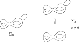
Figure 1. $\Sigma_{x}$.

Let up take $\mathfrak{Y}=\mathcal{C}$ and $\mathfrak{X}=D^{2}({\epsilon})$. For $x\in\mathfrak{X}$ we put $X_{x}=\pi^{-1}(x)\subset\mathcal{C}$. Note:

1. If $x,y\neq 0$ then there exists a unique bi-holomorphic map $X_{x}\to X_{y}$.

2. If $x=y=0$ then the set of bi-holomorphic maps $X_{x}\to X_{y}$ is identified with the set of all affine transformations of ${\mathbb{C}}$, (that is, the maps of the form $z\to az+b$).

3. If $x=0$, $y\neq 0$ then there exist no bi-holomorphic map $X_{x}\to X_{y}$.

For $x\in\mathfrak{X}$ we consider the set of the pairs $(\varphi,y)$ such that $y\in\mathfrak{X}$ and $\varphi:X_{x}\to X_{y}$ is a bi-holomorphic map. (1)(2)(3) above imply that the complex dimension of the space of such pairs is $2$ if $x=0$ and $1$ if $x\neq 0$. Therefore in this case the map ${\rm Pr}_{s}$ can not be a submersion from a complex manifold.

We will study moduli spaces of marked curves. So we include marking to Definition 2.10 as follows.

Definition 2.16.

A marked family of complex analytic spaces parametrized by $\mathfrak{G}$, is a triple $(\widetilde{\mathfrak{G}},\mathscr{F},\vec{\mathfrak{T}})$, where $(\widetilde{\mathfrak{G}},\mathscr{F})$ is a family of complex analytic spaces parametrized by $\mathfrak{G}$ and $\vec{\mathfrak{T}}=(\mathfrak{T}_{1},\dots,\mathfrak{T}_{\ell})$ such that $\mathfrak{T}_{i}:\mathcal{OB}\to\widetilde{\mathcal{OB}}$ are holomorphic maps with the following properties.

1. $\mathscr{F}_{ob}\circ\mathfrak{T}_{i}={\rm id}$.

2. Let $\tilde{\varphi}\in\widetilde{\mathcal{MOR}}$ and $\tilde{x}=\widetilde{\rm Pr}_{s}(\tilde{\varphi})$, $x=\mathscr{F}_{ob}(\tilde{x})$. Suppose $\tilde{x}=\mathfrak{T}_{i}(x)$. Then

   $$\widetilde{\rm Pr}_{t}(\tilde{\varphi})=\mathfrak{T}_{i}({\rm Pr}_{t}(\varphi)).$$

Condition (2) is rephrased as the commutativity of the next diagram.

(2.16) $$\begin{CD}\mathscr{F}^{-1}_{ob}(x)@ >{\tilde{\varphi}}>>\mathscr{F}^{-1}_{ob}(y)\\ @ A{\mathfrak{T}_{i}}AA@ AA{\mathfrak{T}_{i}}A\\ x@ >{\varphi}>>y.\end{CD}$$

Construction 2.17.

Let $\pi:\mathfrak{Y}\to\mathfrak{X}$ be a proper, surjective and flat holomorphic map between complex manifolds and $\mathfrak{T}_{i}:\mathfrak{X}\to\mathfrak{Y}$ holomorphic sections for $i=1,\dots,\ell$. We put $X_{x}=\pi^{-1}(x)$ for $x\in X$. We replace (2.15) by

(2.17) $$\{(x,y,\varphi)\mid x,y\in X, \,\,\,\varphi:X_{x}\to X_{y},\varphi(\mathfrak{T}_{i}(x))=\mathfrak{T}_{i}(y),i=1,\dots,\ell\,\,\text{and}$$

$$\text{$\varphi$ is an isomorphism of complex analytic spaces.}\}$$

We define $\mathcal{MOR}=(\ref{mortal2})$. We assume that it is a complex manifold. The maps ${\rm Pr}_{s}$, ${\rm Pr}_{t}$, which are defined by the same formula as Construction 2.13, are assumed to be submersions. We then obtain $\mathfrak{G}$, $\widetilde{\mathfrak{G}}$ and $\mathscr{F}$ in the same way.

Then together with $\mathfrak{T}_{i}$, the pair $(\widetilde{\mathfrak{G}},\mathscr{F})$ defines a marked family of complex analytic spaces parametrized by $\mathfrak{G}$.

We next define a morphism between families of complex analytic spaces.

Definition 2.18.

Let $(\widetilde{\mathfrak{G}}^{(j)},\mathscr{F}^{(j)})$ be a family of complex analytic spaces parametrized by ${\mathfrak{G}}^{(j)}$ for $j=1,2$. A morphism from $(\widetilde{\mathfrak{G}}^{(1)},\mathscr{F}^{(1)},{\mathfrak{G}}^{(1)})$ to $(\widetilde{\mathfrak{G}}^{(2)},\mathscr{F}^{(2)},{\mathfrak{G}}^{(2)})$ is by definition a pair $(\widetilde{\mathcal{H}},\mathcal{H})$ such that:

1. $\widetilde{\mathcal{H}}:\widetilde{\mathfrak{G}}^{(1)}\to\widetilde{\mathfrak{G}}^{(2)}$ and ${\mathcal{H}}:{\mathfrak{G}}^{(1)}\to{\mathfrak{G}}^{(2)}$ are morphisms such that the next diagram commutes.

   (2.18) $$\begin{CD}\widetilde{\mathfrak{G}}^{(1)}@ >{\widetilde{\mathcal{H}}}>>\widetilde{\mathfrak{G}}^{(2)}\\ @ V{\mathscr{F}^{(1)}}VV@ VV{\mathscr{F}^{(2)}}V\\ {\mathfrak{G}}^{(1)}@ >{\mathcal{H}}>>{\mathfrak{G}}^{(2)}.\end{CD}$$

2. The next diagram is a cartesian square.

   (2.19) $$\begin{CD}\widetilde{\mathcal{OB}}^{(1)}@ >{\widetilde{\mathcal{H}}_{ob}}>>\widetilde{\mathcal{OB}}^{(2)}\\ @ V{\mathscr{F}^{(1)}_{ob}}VV@ VV{\mathscr{F}^{(2)}_{ob}}V\\ {\mathcal{OB}}^{(1)}@ >{\mathcal{H}_{ob}}>>{\mathcal{OB}}^{(2)}.\end{CD}$$

Note Item (2) implies that for each $x\in{\mathcal{OB}}^{(1)}$, the restriction of $\widetilde{\mathcal{H}}_{ob}$ induces an isomorphism

$$({\mathscr{F}^{(1)}_{ob}})^{-1}(x)\cong({\mathscr{F}^{(2)}_{ob}})^{-1}(\mathcal{H}_{ob}(x))$$

In case $(\widetilde{\mathfrak{G}}^{(j)},\mathscr{F}^{(j)},\vec{\mathfrak{T}}^{(j)})$ is a family of marked complex analytic spaces parametrized by ${\mathfrak{G}}^{(j)}$ for $j=1,2$, a morphism between them is a pair $(\widetilde{\mathcal{H}},\mathcal{H})$ satisfying (1)(2) and

1. $\widetilde{\mathcal{H}}_{ob}\circ\vec{\mathfrak{T}}^{(1)}_{i}=\vec{\mathfrak{T}}^{(2)}_{i}\circ{\mathcal{H}}_{ob}.$

Example 2.19.

Let $(\widetilde{\mathfrak{G}},\mathscr{F})$ be a family of complex analytic spaces parametrized by ${\mathfrak{G}}$ and $\mathcal{U}$ an open set of $\mathcal{OB}$. We put $\widetilde{\mathcal{U}}=\mathscr{F}_{ob}^{-1}(\mathcal{U})\subset\widetilde{\mathcal{OB}}$. We consider restrictions ${\mathfrak{G}}|_{\mathcal{U}}$ of ${\mathfrak{G}}$ and $\widetilde{\mathfrak{G}}|_{\widetilde{\mathcal{U}}}$ of $\widetilde{\mathfrak{G}}$.

The restriction of $\mathscr{F}$ defines a morphism $\mathscr{F}|_{\widetilde{\mathcal{U}}}:\widetilde{\mathfrak{G}}|_{\widetilde{\mathcal{U}}}\to\widetilde{\mathfrak{G}}$.

The pair $(\widetilde{\mathfrak{G}}|_{\widetilde{\mathcal{U}}},\mathscr{F}|_{\widetilde{\mathcal{U}}})$ becomes a family of complex analytic spaces parametrized by ${\mathfrak{G}}|_{\mathcal{U}}$. We call it the restriction of $(\widetilde{\mathfrak{G}},\mathscr{F},\mathcal{G})$ to $\mathcal{U}$.

The obvious inclusion defines a morphism $(\widetilde{\mathfrak{G}}|_{\widetilde{\mathcal{U}}},\mathscr{F}|_{\widetilde{\mathcal{U}}},{\mathfrak{G}}|_{\mathcal{U}})\to(\widetilde{\mathfrak{G}},\mathscr{F},{\mathfrak{G}})$ of families of complex analytic spaces. We call it an open inclusion of families of complex analytic varieties.

The version with marking is similar.

Example 2.20.

Let $\pi:\mathfrak{Y}\to\mathfrak{X}$ be a holomorphic map and $\mathfrak{X}^{\prime}\to\mathfrak{X}$ a holomorphic map. We put $\mathfrak{Y}^{\prime}=\mathfrak{Y}\times_{\mathfrak{X}}\mathfrak{X}^{\prime}$ and assume $\mathfrak{Y}^{\prime}$ is a complex manifold. Suppose the assumptions in Construction 2.13 is satisfied both for $\pi:\mathfrak{Y}\to\mathfrak{X}$ and $\pi^{\prime}:\mathfrak{Y}^{\prime}\to\mathfrak{X}^{\prime}$.

Then the morphism from the families induced by $\pi^{\prime}:\mathfrak{Y}^{\prime}\to\mathfrak{X}^{\prime}$ to the families induced by $\pi:\mathfrak{Y}\to\mathfrak{X}$ is obtained in an obvious way.

Lemma 2.21.

Let $(\widetilde{\mathfrak{G}}^{(j)},\mathscr{F}^{(j)})$ be a family of complex analytic spaces parametrized by ${\mathfrak{G}}^{(j)}$ for $j=1,2$, and $(\widetilde{\mathcal{H}}^{(k)},\mathcal{H}^{(k)})$ a morphism from $(\widetilde{\mathfrak{G}}^{(1)},\mathscr{F}^{(1)},{\mathfrak{G}}^{(1)})$ to $(\widetilde{\mathfrak{G}}^{(2)},\mathscr{F}^{(2)},{\mathfrak{G}}^{(2)})$ for $k=1,2$.

Suppose $\mathcal{H}^{(1)}$ is conjugate to $\mathcal{H}^{(2)}$. Then $\widetilde{\mathcal{H}}^{(1)}$ is conjugate to $\widetilde{\mathcal{H}}^{(2)}$.

Proof.

Let $\mathcal{T}$ be a natural transformation from $\mathcal{H}^{(1)}$ to $\mathcal{H}^{(2)}$.

Let $\tilde{x}\in\widetilde{\mathcal{OB}}$. We put $x=\mathscr{F}_{ob}(\tilde{x})$ and $y={\rm Pr}_{t}(\mathcal{T}(x))$ Then $\mathcal{T}(x)$ induces

$$\mathcal{T}(x):\mathscr{F}_{ob}^{-1}(x)\to\mathscr{F}_{ob}^{-1}(y).$$

by (2.13). We put

$$\tilde{y}=\mathcal{T}(x)(\tilde{x}).$$

Using the cartesian square (2.12) there exists a unique $\widetilde{\mathcal{T}}(\tilde{x})\in\widetilde{\mathcal{MOR}}$ such that

$$\mathscr{F}_{mor}(\widetilde{\mathcal{T}}(\tilde{x}))=\mathcal{T}(x)\qquad\widetilde{{\rm Pr}_{s}}(\widetilde{\mathcal{T}}(\tilde{x}))=\tilde{x},\qquad\widetilde{{\rm Pr}_{t}}(\widetilde{\mathcal{T}}(\tilde{x}))=\tilde{y}.$$

Using the cartesian square (2.12) again it is easy to check that $\widetilde{\mathcal{T}}$ is a natural transformation from $\widetilde{\mathcal{H}}^{(1)}$ to $\widetilde{\mathcal{H}}^{(2)}$. ∎

Definition 2.22.

We say $(\widetilde{\mathfrak{G}}^{(1)},\mathscr{F}^{(1)})$ is conjugate to $(\widetilde{\mathfrak{G}}^{(2)},\mathscr{F}^{(2)})$ if the assumption of Lemma 2.21 is satisfied.

Our main interest in this paper is local theory. We define the next notion for this purpose.

Definition 2.23.

Let $(X,\vec{z})$ be a pair of complex analytic space $X$ and an $\ell$-tuple of mutually distinct smooth points $\vec{z}=(z_{1},\dots,z_{\ell})$. A deformation of $(X,\vec{z})$ is by definition an object $(\widetilde{\mathfrak{G}},\mathscr{F},{\mathfrak{G}},\vec{\mathfrak{T}},o,\iota)$ with the following properties.

1. The triple $(\widetilde{\mathfrak{G}},\mathscr{F},\vec{\mathfrak{T}})$ is a marked family of complex variety parametrized by ${\mathfrak{G}}$.

2. $o\in\mathcal{OB}$.

3. $\iota:X\to\mathscr{F}_{ob}^{-1}(o)$ is a bi-holomorphic map.

4. $\mathfrak{T}_{i}(o)=\iota(z_{i})$.

Let $\mathcal{G}^{(j)}=(\widetilde{\mathfrak{G}}^{(j)},\mathscr{F}^{(j)},{\mathfrak{G}}^{(j)},\vec{\mathfrak{T}}^{(j)},o^{(j)},\iota^{(j)})$ be a deformation of $(X,\vec{z})$ for $j=1,2$. A strict morphism from $\mathcal{G}^{(1)}$ to $\mathcal{G}^{(2)}$ is a morphism from $(\widetilde{\mathcal{H}},\mathcal{H})$ from $\mathscr{F}^{(1)},{\mathfrak{G}}^{(1)},\vec{\mathfrak{T}}^{(1)}$ to $\mathscr{F}^{(2)},{\mathfrak{G}}^{(2)},\vec{\mathfrak{T}}^{(2)}$ such that:

1. ${\mathfrak{T}}^{(2)}_{i}\circ\mathcal{H}=\widetilde{\mathcal{H}}\circ{\mathfrak{T}}^{(1)}_{i}.$

2. $o^{(2)}=\mathcal{H}_{ob}(o^{(1)})$.

3. $\widetilde{\mathcal{H}}_{ob}\circ\iota^{(1)}=\iota^{(2)}.$

Let $\mathcal{G}=(\widetilde{\mathfrak{G}},\mathscr{F},{\mathfrak{G}},\vec{\mathfrak{T}},o,\iota)$ be a deformation of $(X,\vec{z})$ and $\mathcal{U}$ is an open neighboorhood $o$ in $\mathcal{OB}$. We define the restriction of $\mathcal{G}$ to $\mathcal{U}$ in an obvious way and denote it by $\mathcal{G}|_{\mathcal{U}}$.

A morphism from $\mathcal{G}^{(1)}$ to $\mathcal{G}^{(2)}$ is a strict morphism from $\mathcal{G}^{(1)}|_{\mathcal{U}}$ to $\mathcal{G}^{(2)}$ for a certain open neighboorhood $o$ in $\mathcal{OB}^{(1)}$.

Two morphisms are said to coincide as germs if they coincides after further restricting to a smaller neighborhood of $o$ in $\mathcal{OB}^{(1)}$.

We can compose two strict morphisms or two morphisms in an obvious way. There is an identity morphism from $\mathcal{G}$ to itself.

A morphism $\mathscr{H}=(\widetilde{\mathcal{H}},\mathcal{H};\mathcal{U})$ from $\mathcal{G}^{(1)}$ to $\mathcal{G}^{(2)}$ is said to be an isomorphism, if there exists a morphism $\mathscr{H}^{\prime}=(\widetilde{\mathcal{H}}^{\prime},\mathcal{H}^{\prime};\mathcal{U}^{\prime})$ from $\mathcal{G}^{(1)}$ to $\mathcal{G}^{(2)}$ such that the compositions $\mathscr{H}^{\prime}\circ\mathscr{H}$ and $\mathscr{H}\circ\mathscr{H}^{\prime}$ coincides with the identity morphisms as germs.

A germ of deformation of $(X,\vec{z})$ is an isomorphism class with respect to the isomorphism defined above.

Definition 2.24.

Let $\mathcal{G}^{(j)}=(\widetilde{\mathfrak{G}}^{(j)},\mathscr{F}^{(j)},{\mathfrak{G}}^{(j)},\vec{\mathfrak{T}}^{(j)},o^{(j)},\iota^{(j)})$ be a deformation of $(X,\vec{z})$ for $j=1,2$. Two strict morphisms $(\widetilde{\mathcal{H}},\mathcal{H})$, $(\widetilde{\mathcal{H}}^{\prime},\mathcal{H}^{\prime})$ from $\mathcal{G}^{(1)}$ to $\mathcal{G}^{(2)}$ are said to be conjugate if there exists a pair of natural transformation $(\widetilde{\mathcal{T}},\mathcal{T})$ from $(\widetilde{\mathcal{H}},\mathcal{H})$ as in Lemma 2.21 such that:

1. ${\mathfrak{T}}^{(2)}_{i}\circ\mathcal{T}=\widetilde{\mathcal{T}}\circ{\mathfrak{T}}^{(2)}_{i}$.

2. $\mathcal{T}_{ob}(o^{(1)})=o^{(2)}$.

3. $\widetilde{\mathcal{T}}_{ob}\circ\iota^{(1)}=\iota^{(2)}$.

Two morphisms from $\mathcal{G}^{(1)}$ to $\mathcal{G}^{(2)}$ are said to be conjugate if they are conjugate as strict morphisms after restricting to a certain open neighborhood of $o^{(1)}$.

3. Universal deformations of unstable marked curves

In this section we specialize to the case of family of one dimensional complex varieties and show existence and uniqueness of a universal family for certain class of deformations.

3.1. Universal deformation and its uniqueness

Let $\pi:\mathfrak{Y}\to\mathfrak{X}$ be a holomorphic map and $x\in\mathfrak{X}$. We put $\Sigma_{x}=\pi^{-1}(x)$.

Definition 3.1.

We say $\pi:\mathfrak{Y}\to\mathfrak{X}$ is a nodal family and $\Sigma_{x}$ is a nodal curve if for each $y\in\Sigma_{x}$ one of the following holds.

1. $D_{y}\pi:T_{y}\mathfrak{Y}\to T_{x}\mathfrak{X}$ is surjective. $\dim_{{\mathbb{C}}}{\rm Ker}\,D_{x}\pi=1$.

2. Let $\mathscr{I}_{x}$ be the ideal of germs of holomorphic functions on $X$ at $x$ which vanish at $x$. Then we have

   $$\frac{\mathcal{O}_{y}}{\pi^{*}\mathscr{I}_{x}}=\frac{{\mathbb{C}}\{z,w\}}{(zw)}.$$

   Here $\mathcal{O}_{y}$ is the ring of germs of holomorphic functions of $\mathfrak{Y}$ at $y$. The ring ${\mathbb{C}}\{z,w\}$ is the convergent power series ring of two variables.

We say $y$ is a regular point if Item (1) happens and $y$ is a nodal point if Item (2) happens.

Definition 3.2.

Let $(\widetilde{\mathfrak{G}},\mathscr{F})$ be a family of complex analytic varieties parametrized by ${\mathfrak{G}}$. We say that $(\widetilde{\mathfrak{G}},\mathscr{F},{\mathfrak{G}})$ is a family of nodal curves if $\mathscr{F}_{ob}:\widetilde{\mathcal{OB}}\to\mathcal{OB}$ is a nodal family.

A marked family $(\widetilde{\mathfrak{G}},\mathscr{F},\vec{\mathfrak{T}})$ of complex analytic spaces parametrized by $\mathfrak{G}$ is said to be a family of marked nodal curves if $(\widetilde{\mathfrak{G}},\mathscr{F},{\mathfrak{G}})$ is a family of nodal curves and the following holds.

1. For any $x\in\mathcal{OB}$ the point $\mathfrak{T}_{i}(x)\in\mathscr{F}_{ob}^{-1}(x)$ is a regular point of $\mathscr{F}_{ob}^{-1}(x)$.

2. If $i\neq j$ and $x\in\mathcal{OB}$, then $\mathfrak{T}_{i}(x)\neq\mathfrak{T}_{j}(x)$.

Definition 3.3.

Let $(\widetilde{\mathfrak{G}},\mathscr{F})$ be a family of complex analytic spaces parametrized by ${\mathfrak{G}}$. We say that $(\widetilde{\mathfrak{G}},\mathscr{F},{\mathfrak{G}})$ is minimal at $o$ if the following holds.

If $\varphi\in\mathcal{MOR}$ with ${\rm Pr}_{s}(\varphi)=o$ then ${\rm Pr}_{t}(\varphi)=o$.

Definition 3.4.

Let $(\Sigma,\vec{z})$ be a marked nodal curve and $\mathcal{G}=(\widetilde{\mathfrak{G}},\mathscr{F},{\mathfrak{G}},\vec{\mathfrak{T}},o,\iota)$ a deformation of $(\Sigma,\vec{z})$. We say that $\mathcal{G}$ is a universal deformation of $(\Sigma,\vec{z})$ if the following holds.

1. $(\widetilde{\mathfrak{G}},\mathscr{F},{\mathfrak{G}},\vec{\mathfrak{T}})$ is a family of nodal curves and is minimal at $o$.

2. For any deformation $\mathcal{G}^{\prime}=(\widetilde{\mathfrak{G}^{\prime}},\mathscr{F}^{\prime},{\mathfrak{G}}^{\prime},\vec{\mathfrak{T}}^{\prime},o^{\prime},\iota^{\prime})$ of $(\Sigma,\vec{z})$ such that $(\widetilde{\mathfrak{G}}^{\prime},\mathscr{F}^{\prime},{\mathfrak{G}}^{\prime},\vec{\mathfrak{T}}^{\prime})$ is a family of nodal curves, there exists a morphism $(\widetilde{\mathcal{H}},\mathcal{H})$ (Definition 2.23) from $\mathcal{G}^{\prime}$ to $\mathcal{G}$.

3. In the situation of Item (2) if $(\widetilde{\mathcal{H}}^{\prime},\mathcal{H}^{\prime})$ is another morphism then $\mathcal{H}^{\prime}$ is conjugate to $\mathcal{H}$.

The main result of this section is the following.

Theorem 3.5.

For any marked nodal curve $(\Sigma,\vec{z})$ there exists its universal deformation $\mathcal{G}=(\widetilde{\mathfrak{G}},\mathscr{F},{\mathfrak{G}},\vec{\mathfrak{T}},o,\iota)$.

If $\mathcal{G}^{(j)}=(\widetilde{\mathfrak{G}}^{(j)},\mathscr{F}^{(j)},{\mathfrak{G}}^{(j)},\vec{\mathfrak{T}}^{(j)},o^{(j)},\iota^{(j)})$, $j=1,2$ are both universal deformations of $(\Sigma,\vec{z})$ then they are isomorphic as germs in the sense of Definition 2.23.

Remark 3.6.

If $(\Sigma,\vec{z})$ is marked stable curve, that is, the group of its automorphisms is a finite group, the universal deformation $\mathcal{G}=(\widetilde{\mathfrak{G}},\mathscr{F},{\mathfrak{G}},\vec{\mathfrak{T}},o,\iota)$ is étale. Namely ${\rm Pr}_{s}:\mathcal{MOR}\to\mathcal{OB}$ is a local diffeomorphism. Theorem 3.5 in this case follows from the classical result that the moduli space of marked stable curve is an orbifold. (In some case this orbifold is not effective.) Orbifold is a classical and well-established notion in differential geometry [Sa]. The fact that orbifold can be studied using the language of étale groupoid is also classical [Ha].

In the case when $(\Sigma,\vec{z})$ is not stable, $\dim\mathcal{MOR}>\dim\mathcal{OB}$ and so ${\mathfrak{G}}$ is not étale. Therefore using the language of Lie groupoid is more important in this case than the case of orbifold.

It seems unlikely that there is a literature which proves a similar result as Theorem 3.5 by the method of differential geometry. Something equivalent to Theorem 3.5 is known in algebraic geometry using the terminology of Artin Stack ([Ar]). See [Man, Chapter V 3.2.1 and 5.5.3]. For our purpose of proving Theorem 5.3, differential geometric approach is important. So we provide a detailed proof of Theorem 3.5 below.

Proof.

In this subsection we prove the uniqueness. The existence will be proved in the next subsection.

Suppose $\mathcal{G}^{(j)}=(\widetilde{\mathfrak{G}}^{(j)},\mathscr{F}^{(j)},{\mathfrak{G}}^{(j)},\vec{\mathfrak{T}}^{(j)},o^{(j)},\iota^{(j)})$, $j=1,2$ are both universal deformations of $(\Sigma,\vec{z})$. Then by Definition 3.4 (2), there exists a morphism $(\widetilde{\mathcal{H}},\mathcal{H})$ from $\mathcal{G}^{(1)}$ to $\mathcal{G}^{(2)}$ and also a morphism $(\widetilde{\mathcal{H}}^{\prime},\mathcal{H}^{\prime})$ from $\mathcal{G}^{(2)}$ to $\mathcal{G}^{(1)}$.

The composition $(\widetilde{\mathcal{H}}^{\prime},\mathcal{H}^{\prime})\circ(\widetilde{\mathcal{H}},\mathcal{H})$ is a morphism from $\mathcal{G}^{(1)}$ to itself. By Definition 3.4 Item (3) it is conjugate to the identity morphism.

Lemma 3.7.

A morphism from $(\widetilde{\mathfrak{G}},\mathscr{F},{\mathfrak{G}})$ to itself which is conjugate to the identity morphism is necessarily an isomorphism in a neighborhood of $o$, if $(\widetilde{\mathfrak{G}},\mathscr{F},{\mathfrak{G}})$ is minimal at $o$.

Postponing the proof of the lemma we continue the proof.

By the lemma we replace $(\widetilde{\mathcal{H}}^{\prime},\mathcal{H}^{\prime})$ if necessary and may assume that $(\widetilde{\mathcal{H}}^{\prime},\mathcal{H}^{\prime})\circ(\widetilde{\mathcal{H}},\mathcal{H})={\rm id}$.

By the same argument the composition $(\widetilde{\mathcal{H}},\mathcal{H})\circ(\widetilde{\mathcal{H}}^{\prime},\mathcal{H}^{\prime})$ is an isomorphism. We may replace $(\widetilde{\mathcal{H}}^{\prime},\mathcal{H}^{\prime})$ by $(\widetilde{\mathcal{H}}^{\prime\prime},\mathcal{H}^{\prime\prime})$ and find that $(\widetilde{\mathcal{H}},\mathcal{H})\circ(\widetilde{\mathcal{H}}^{\prime\prime},\mathcal{H}^{\prime\prime})={\rm id}$.

Then by a standard argument $(\widetilde{\mathcal{H}}^{\prime},\mathcal{H}^{\prime})=(\widetilde{\mathcal{H}}^{\prime\prime},\mathcal{H}^{\prime\prime}).$

Thus to complete the proof of uniqueness it remains to prove the lemma. ∎

Proof of Lemma 3.7.

Let $(\widetilde{\mathcal{H}},\mathcal{H})$ be a morphism from $(\widetilde{\mathfrak{G}},\mathscr{F},{\mathfrak{G}})$ to itself, which is conjugate to the identity.

By Lemma 2.8 there exists $\mathcal{T}:\mathcal{OB}\to\mathcal{MOR}$ such that $\mathcal{H}=\mathfrak{conj}^{\mathcal{T}}$.

Sublemma 3.8.

The map $\mathcal{H}_{ob}:\mathcal{OB}\to\mathcal{OB}$ is a diffeomorphism on a neighborhood of $o$.

Proof.

By minimality at $o$, we find $\mathcal{H}_{ob}(o)=o$. Let $\varphi_{o}=\mathcal{T}(o)$. We have

(3.1) $$\mathcal{H}_{ob}(x)={\rm Pr}_{t}(\mathcal{T}(x)).$$

Using implicit function theorem we may identify a neighborhood of $\mathcal{T}(o)$ in $\mathcal{MOR}$ with $\mathcal{U}\times\mathcal{V}$ such that $\mathcal{V}\subset{\rm Pr}_{s}^{-1}(o)$ is an open neighborhood of $\mathcal{T}(o)$, $\mathcal{U}$ is an open neighborhood of $o$ in $\mathcal{OB}$ and ${\rm Pr}_{s}:\mathcal{U}\times\mathcal{V}\to\mathcal{OB}$ is the projection. We remark that the derivative in the $\mathcal{V}$ direction of ${\rm Pr}_{t}:\mathcal{U}\times\mathcal{V}\to\mathcal{OB}$ is zero on $\{o\}\times\mathcal{V}$ by minimality. On the other hand the derivative in the $\mathcal{U}$ direction of ${\rm Pr}_{t}$ at $(o,\mathcal{T}(o))$ is invertible. This is because ${\rm Pr}_{t}$ is a submersion and the derivative in the $\mathcal{V}$ direction is zero.

Thus derivative of (3.1) is invertible at $o$. In fact

$$\mathcal{H}_{ob}(x)={\rm Pr}_{t}(x,\mathcal{T}^{\prime}(x))$$

for some $\mathcal{T}^{\prime}:\mathcal{U}\to\mathcal{V}$. Sublemma 3.8 now follows from inverse function theorem. ∎

Thus we proved that $\mathcal{H}_{ob}$ is invertible. It is easy to see that it implies that $\mathcal{H}$ is invertible.

By Lemma 2.21, $\widetilde{\mathcal{H}}$ is conjugate to the identity morphism. We can use it in the same way as above to show that $\widetilde{\mathcal{H}}$ is an isomorphism if we restrict to a smaller neighborhood of $o$. The proof of Lemma 3.7 is complete. ∎

3.2. Existence of the universal deformation

In this section we prove the existence part of Theorem 3.5. We use the existence of universal deformation of stable marked nodal curve, which was well established long time ago and by now well-known, and use it to study unstable case.

Let $(\Sigma,\vec{z})$ be a marked nodal curve. We decompose $\Sigma$ into irreducible components

(3.2) $$\Sigma=\bigcup_{a\in\mathcal{A}}\Sigma_{a}.$$

We regard the intersection $\vec{z}\cap\Sigma_{a}$ and all the nodal points on $\Sigma_{a}$ as marked points of $\Sigma_{a}$ and denote it by $\vec{z}_{a}$. We put $\vec{z}_{a}=(z_{a,1},\dots,z_{a,\ell_{a}})$. We recall that $(\Sigma_{a},\vec{z}_{a})$ is stable unless one of the following holds:

1. The genus of $\Sigma_{a}$ is $0$ and $\#\vec{z}_{a}=0$.

2. The genus of $\Sigma_{a}$ is $0$ and $\#\vec{z}_{a}=1$.

3. The genus of $\Sigma_{a}$ is $0$ and $\#\vec{z}_{a}=2$.

4. The genus of $\Sigma_{a}$ is $1$ and $\#\vec{z}_{a}=0$.

Note in case (US.0), $\Sigma=\Sigma_{a}$ and it is easy to construct a universal deformation. (In fact $\mathcal{OB}$ consists of one point, $\mathcal{MOR}=PSL(2;{\mathbb{C}})$. $\widetilde{\mathfrak{G}}$ is defined by using $PSL(2;{\mathbb{C}})$ action on $S^{2}$.) In case (US.3), again $\Sigma=\Sigma_{a}$. We can define universal deformation easily also. ($\mathcal{OB}$ is an open subset of the moduli space of elliptic curves. Other objects can be obtained by applying Construction 2.17 to the universal family of elliptic curves.)

Therefore we consider the case when all the unstable components are either of type (US.1) or (US.2).

Let $\mathcal{A}_{s}$ be the subset of $\mathcal{A}$ consisting of elements $a$ such that $(\Sigma_{a},\vec{z}_{a})$ is stable. We put $\mathcal{A}_{u}=\mathcal{A}\setminus\mathcal{A}_{s}$.

Suppose $(\Sigma_{a},\vec{z}_{a})$ is a stable curve. Let $g_{a}$ be its genus and $\ell_{a}=\#\vec{z}_{a}$. We consider the moduli space $\mathcal{M}_{g_{a},\ell_{a}}$ of stable curves with genus $g_{a}$ and with $\ell_{a}$ marked points. $\mathcal{M}_{g_{a},\ell_{a}}$ is an orbifold. (In some exceptional case it is not effective.) Let $\mathcal{V}_{a}/\mathcal{G}_{a}$ be a neighborhood of $(\Sigma_{a},\vec{z}_{a})$ in $\mathcal{M}_{g_{a},\ell_{a}}$. Here $\mathcal{G}_{a}$ is a finite group which is the group of automorphisms of $(\Sigma_{a},\vec{z}_{a})$. Namely

$$\mathcal{G}_{a}=\{v:\Sigma_{a}\to\Sigma_{a}\mid\text{$v$ is bi-holomorphic},\,\,v(z_{a,i})=z_{a,i}\}.$$

$\mathcal{V}_{a}$ is a smooth complex manifold on which a finite group $\mathcal{G}_{a}$ acts. We have a universal family

(3.3) $$\pi_{a}:\mathcal{C}_{a}\to\mathcal{V}_{a}$$

where $\mathcal{C}_{a}$ is a complex manifold and $\pi_{a}$ is a proper submersion. The group $\mathcal{G}_{a}$ acts on $\mathcal{C}_{a}$ and $\pi_{a}$ is $\mathcal{G}_{a}$ equivariant. We also have holomorphic maps

(3.4) $$\mathfrak{t}_{a,i}:\mathcal{V}_{a}\to\mathcal{C}_{a}$$

for $i=1,\dots,\ell_{a}$, such that $\pi_{a}\circ\mathfrak{t}_{a,i}={\rm id}$ and $\mathfrak{t}_{a,i}$ is $\mathcal{G}_{a}$ equivariant. Moreover $\mathfrak{t}_{a,i}(x)\neq\mathfrak{t}_{a,j}(x)$ for $x\in\mathcal{V}_{a}$, $i\neq j$. Finally the marked Riemannn surface

$$(\pi_{a}^{-1}(x),(\mathfrak{t}_{a,1}(x),\dots,\mathfrak{t}_{a,\ell_{a}}(x)))$$

is a representative of the element $[x]\in\mathcal{V}_{a}/\mathcal{G}_{a}\subset\mathcal{M}_{g_{a},\ell_{a}}$. Existence of such $\mathcal{G}_{a},\mathcal{V}_{a},\mathcal{C}_{a},\pi_{a},\mathfrak{t}_{a,i}$ is classical. (See [ACG] for example. This one dimensional and local version of deformation theory of complex structure had been known in 19th century.)

Suppose $(\Sigma_{a},\vec{z}_{a})$ is unstable. We put $\mathcal{V}_{a}={\rm point}$. The group of automorphisms $\mathcal{G}_{a}$ is ${\mathbb{C}}^{*}={\mathbb{C}}\setminus\{0\}$ if (US.1) is satisfied. The group of automorphisms $\mathcal{G}_{a}$ consists of affine maps $z\mapsto az+b$ in case (US.2) is satisfied. (Here we identify $(\Sigma_{a},\vec{z}_{a})=({\mathbb{C}}\cup\{\infty\},\infty)$.

We put

(3.5) $$\mathcal{G}=\{v:\Sigma\to\Sigma\mid\text{$v$ is bi-holomorphic},\,\,v(z_{i})=z_{i}\}.$$

We then have an exact sequence of groups:

(3.6) $$1\to\prod_{a\in\mathcal{A}}\mathcal{G}_{a}\to\mathcal{G}\to\mathscr{H}\to 1.$$

Here $\mathscr{H}$ is a finite group. The group $\mathscr{H}$ is a subgroup of the automorphism group of the dual graph of $\Sigma$. (Here the dual graph is defined as follows. We associate a vertex to each of the irreducible components of $\Sigma$. We associate an edge to each of the nodal points. The vertices of an edge is one associated to the irreducible components containing that nodal points. See Figure 2 below.)

Figure 2. Dual graph to nodal curve

We put $\overline{\mathcal{G}}=\pi_{0}(\mathcal{G})$. Then we have an exact sequence

(3.7) $$1\to\prod_{a\in\mathcal{A}_{s}}\mathcal{G}_{a}\to\overline{\mathcal{G}}\to\mathscr{H}\to 1.$$

We put

(3.8) $$\mathcal{V}_{0}=\prod_{a\in\mathcal{A}_{s}}\mathcal{V}_{a}.$$

Let $o\in\mathcal{V}_{0}$ be an element corresponding to $\Sigma$.

The group $\overline{\mathcal{G}}$ acts on $\mathcal{V}_{0}$ in an obvious way. For each $x=(x_{a})_{a\in\mathcal{A}_{s}}$ we define $\Sigma(x)$ as follows. We take $\Sigma(x_{a})=\pi^{-1}(x_{a})$ for $a\in\mathcal{A}_{s}$. If $a\in\mathcal{A}_{u}$ we take $\Sigma_{a}$. We glue

$$\coprod_{a\in\mathcal{A}_{s}}\Sigma(x_{a})\sqcup\coprod_{a\in\mathcal{A}_{u}}\Sigma_{a}$$

at their marked points in exactly the same way as $\Sigma$. We then obtain a nodal curve $\Sigma(x)$. We define

$$\mathcal{C}_{0}=\coprod_{x\in\mathcal{V}_{0}}\Sigma(x)\times\{x\}.$$

We have an obvious projection

(3.9) $$\pi:\mathcal{C}_{0}\to\mathcal{V}_{0}.$$

$\overline{\mathcal{G}}$ acts on $\mathcal{C}_{0}$ in an obvious way and then (3.9) is a deformation of $\Sigma$ while keeping singularities. Later in (3.10) we will embed $\mathcal{C}_{0}$ to a complex manifold so that $\mathcal{C}_{0}$ is a complex subvariety. The choice of complex structure of $\mathcal{C}_{0}$ then will become clear. Using the map $\mathfrak{t}_{a,i}$ which does not correspond to the nodal point of $\Sigma(x)$ we obtain maps

$$\mathfrak{t}_{j}:\mathcal{V}_{0}\to\mathcal{C}_{0}$$

for $j=1,\dots,\ell$ such that $\pi\circ\mathfrak{t}_{j}={\rm id}$ and that $\mathfrak{t}_{j}$ is $\overline{\mathcal{G}}$ equivariant.

We next include the parameter to smooth nodal points of $\Sigma(x)$. We need to choose a coordinate at each nodal points, in the following sense. Let $D^{2}(r)$ be the open ball of radius $r$ centered at $0$ in ${\mathbb{C}}$.

Definition 3.9.

([FOOO6, Definition 8.1]) An analytic family of coordinates at $\mathfrak{t}_{a,i}$ is a holomorphic map

$$\varphi_{a,i}:\mathcal{V}_{a}\times D^{2}(2)\to\mathcal{C}_{a}$$

such that:

1. $\pi(\varphi_{a,i}(x,z))=x$, for all $z\in D^{2}(2)$.

2. $\varphi_{a,i}(x,0)=\mathfrak{t}_{a,i}(x)$.

3. For each $x$ the map $z\mapsto\varphi_{a,i}(x,z)$ is a bi-holomorphic map from $D^{2}(2)$ to a neighborhood of $\mathfrak{t}_{a,i}(x)$ in $\pi_{a}^{-1}(x)$.

We say that a system $(\varphi_{a,i})_{a\in\mathcal{A}_{s},i=1,\dots,\ell_{a}}$ of analytic families of coordinates are $\overline{\mathcal{G}}$ equivariant if the following holds. Let $\gamma\in\overline{\mathcal{G}}$ and $[\gamma]\in{\mathscr{H}}$. We consider

$${\rm Node}=\{(a,i)\mid\text{$z_{a,i}$ corresponds to a nodal point of $\Sigma$ on $\Sigma_{a}$.}\}$$

Since ${\mathscr{H}}$ acts on the dual graph of $\Sigma$ it acts on ${\rm Node}$ also. Now we require:

1. If $[\gamma](a,i)=(a^{\prime},i^{\prime})$ then

   $$\gamma(\varphi_{a,i}(x,z))=\exp(\theta_{\gamma,a,i}\sqrt{-1})\varphi_{a^{\prime},i^{\prime}}(x,z).$$

   Here $\theta_{a,i}\in{\mathbb{R}}$.

Lemma 3.10.

There exists a $\overline{\mathcal{G}}$ equivariant analytic families of coordinates.

See [FOOO8, Lemma 8.4] for the proof of this lemma.

Remark 3.11.

We use analytic family of coordinates at the marked points corresponding to the nodal points only.

For each $(z,i)\in{\rm Node}$ we take a copy of ${\mathbb{C}}$ and denote it by ${\mathbb{C}}_{(z,i)}$. We fix an orientation of the edges of the dual graph $\Gamma(\Sigma)$ of $\Sigma$. For each edge ${\rm e}$ of $\Gamma(\Sigma)$, that corresponds to the nodal points, let $z_{-,{\rm e}},z_{+,{\rm e}}\in{\rm Node}$ such that the orientation of ${\rm e}$ goes from the vertex corresponding to $z_{-,{\rm e}}$ to the vertex corresponding to $z_{+,{\rm e}}$.

Definition 3.12.

We put

$$\mathcal{V}_{1}=\bigoplus{\mathbb{C}}_{-,{\rm e}}\otimes{\mathbb{C}}_{+,{\rm e}},$$

where the direct sum is taken over all the edges ${\rm e}$ of $\Gamma(\Sigma)$. The element $\gamma\in\overline{\mathscr{G}}$ acts on $\mathcal{V}_{1}$ by sending $w\in{\mathbb{C}}_{-,{\rm e}}^{*}$ (resp. $w\in{\mathbb{C}}^{*}_{+,{\rm e}}$) to $\exp(\theta_{\gamma,a,i}\sqrt{-1})w$ if $z_{-,{\rm e}}=z_{a,i}$ (resp. $\exp(\theta_{\gamma,a^{\prime},i^{\prime}}\sqrt{-1})w$ if $z_{+,{\rm e}}=z_{a^{\prime},i^{\prime}}$).

Construction 3.13.

We put $\mathcal{V}_{+}=\mathcal{V}_{0}\times\mathcal{V}_{1}$. We are going to define a neighborhood $\mathcal{V}$ of $(0,0)$ in $\mathcal{V}_{+}$, a complex manifold $\mathcal{C}$, and a map $\mathcal{C}\to\mathcal{V}$ as follows.

For each $\vec{x}=(x_{a})_{a\in\mathcal{A}_{s}}\in\mathcal{V}_{0}=\prod\mathcal{V}_{a}$ we take

$$\bigcup_{a\in\mathcal{A}_{s}}\Sigma(x_{a})\cup\bigcup_{a\in\mathcal{A}_{u}}\Sigma_{a}.$$

We remove the union of $\varphi_{a,i}(D^{2})$ for all $\varphi_{a,i}$ corresponding to the nodal point. We denote it as $\Sigma(\vec{x})_{0}$. Let

$$\mathcal{C}_{0}=\bigcup_{\vec{x}\in\mathcal{V}_{0}}\left(\Sigma(\vec{x})_{0}\times\{\vec{x}\}\right)$$

and $\mathcal{C}_{0}\to\mathcal{V}_{0}$ the obvious projection. $\mathcal{C}_{0}$ is a complex manifold and the projection is holomorphic. We compactify the fibers of $(\mathcal{C}_{0}\times\mathcal{V}_{1})\to\mathcal{V}$ as follows. Let $\vec{\rho}=(\rho_{\rm e})_{{\rm e}\in\Gamma(\Sigma)}\in\mathcal{V}_{1}$. We put $z_{-,{\rm e}}=z_{a,i}$, $z_{+,{\rm e}}=z_{a^{\prime},i^{\prime}}$ and $r_{\rm e}=|\rho_{\rm e}|$. We consider

$$\left(D^{2}(2)\setminus D^{2}(r_{\rm e})\right)\cup\left(D^{2}(2)\setminus D^{2}(r_{\rm e})\right)$$

and identify $z$ in the first summand with $w$ in the second summand if $zw=\rho_{\rm e}$.

We also identify $z$ with $\varphi_{i,a}(z)$ if $|z|>1$ and $w$ with $\varphi_{i^{\prime},a^{\prime}}(w)$ if $|w|>1$.

Performing this gluing at all the nodal points we obtain $\Sigma(\vec{x},\vec{\rho})$. We put

(3.10) $$\mathcal{C}=\bigcup_{\vec{x}\in\mathcal{V}_{0},\vec{\rho}\in\mathcal{V}_{1}}\Sigma(\vec{x},\vec{\rho})\times\{(\vec{x},\vec{\rho})\}.$$

The natural projection induces a map $\pi:\mathcal{C}\to\mathcal{V}$. It is easy to see from the construction that $\mathcal{C}$ is a complex manifold and $\pi$ is holomorphic. Moreover the fiber of $\pi$ are nodal curves. $\mathfrak{t}_{j}:\mathcal{V}_{0}\to\mathcal{C}_{0}$ can be regarded as a map $\mathfrak{t}_{j}:\mathcal{V}\to\mathcal{C}$ by which $(\pi^{-1}(x);\mathfrak{t}_{1}(x),\dots,\mathfrak{t}_{\ell}(x))$ becomes a marked nodal curve.

The most important part of the proof of Theorem 3.5 is the following:

Proposition 3.14.

Let $\mathcal{MOR}$ be the set of triples $(\varphi,x,y)$ where $x,y\in\mathcal{V}$ and $\varphi:\pi^{-1}(x)\to\pi^{-1}(y)$ an isomorphism such that $\varphi(\mathfrak{t}_{j}(x))=\mathfrak{t}_{j}(y)$ for $j=1,\dots,\ell$. Then

1. $\mathcal{MOR}$ has a structure of a smooth complex manifold.

2. The two projections $\mathcal{MOR}\to\mathcal{V}$, $(\varphi,x,y)\mapsto x$, $(\varphi,x,y)\mapsto y$ are both submersions.

Note by Proposition 3.14 and Constructions 2.13 and 2.17 we obtain a family of marked nodal curves.

Proof.

We first define a topology (metric) on $\mathcal{MOR}$. Note $\mathcal{C}$ and $\mathcal{V}$ are obviously metrizable. We take its metric.

Definition 3.15.

We say $d((\varphi,x,y),(\varphi^{\prime},x^{\prime},y^{\prime}))\leq\epsilon$ if

$$d(x,x^{\prime})\leq\epsilon,\quad d(y,y^{\prime})\leq\epsilon$$

and

$$|d(\varphi(a),\varphi^{\prime}(b))-d(a,b)|\leq\epsilon$$

for $a\in\pi^{-1}(x)$, $b\in\pi^{-1}(x^{\prime})$.

It is easy to see that $d$ defines a metric on $\mathcal{MOR}$.

Definition 3.16.

The minimal stabilization $\vec{w}_{a}$ of an unstable component $(\Sigma_{a},\vec{z}_{a})$ is as follows.

In case (US.1), $\vec{w}_{a}$ consists of (distinct) two points which do not intersect with $\vec{z}_{a}$.

In case (US.2), $\vec{w}_{a}$ consists of one point which does not intersect with $\vec{z}_{a}$.

Note $(\Sigma_{a},\vec{z}_{a}\cup\vec{w}_{a})$ becomes stable. In fact it is a sphere with three marked points and so there is no deformation and no automorphism. The choice of minimal stabilization is unique up to isomorphism.

We add minimal stabilization to each unstable components and obtain a stable marked curve $(\Sigma,\vec{z}\cup\vec{w})$. The next lemma is obvious.

Lemma 3.17.

$\overline{\mathcal{G}}$ acts on $\Sigma$ such that it preserves $\vec{w}$ as a set.

We denote $\vec{w}=\{w_{1},\dots w_{k}\}$. By construction we have sections $\mathcal{S}_{j,0}:\mathcal{V}_{0}\to\mathcal{C}_{0}$ such that $\mathcal{S}_{j,0}(x)$ is identified with $w_{j}$. Using the description of $\Sigma(\vec{x},\vec{\rho})$ we gave above we obtain a marked point $w_{j}(\vec{x},\vec{\rho})$. Thus we obtain holomorphic sections $\mathcal{S}_{j}:\mathcal{V}\to\mathcal{C}$. The next lemma is a consequence of a standard result of the deformation theory of stable nodal curve. (See [ACG].) Let $\overline{\mathcal{G}}_{0}$ be a subgroup of $\overline{\mathcal{G}}$ consisting of elements which fix each point $w_{j}$.

Lemma 3.18.

$((\mathcal{C},\mathcal{V}),\pi,(\mathfrak{T}_{j};j=1,\dots,\ell)\cup(\mathcal{S}_{j};j=1,\dots,k))$ divided by $\overline{\mathcal{G}}_{0}$ is a local universal family of genus $g$ stable curves with $k+\ell$ marked points.

See for example [ACG], [Man] for the definition of universal family of genus $g$ stable curves with $k+\ell$ marked points. Actually it is a special case of Definition 3.4 where ${\rm Pr}_{s}$ and ${\rm Pr}_{t}$ are local diffeomorphisms.

We now start constructing a chart of $\mathcal{MOR}$. We first consider $(\varphi,o,o)$, that is the case when $\varphi:(\Sigma,\vec{z})\to(\Sigma,\vec{z})$ is an automorphism.

Let $U$ be a neighborhood of $\varphi$ in the group of automorphisms of $(\Sigma,\vec{z})$. Let $\mathcal{V}^{\prime}$ be a sufficiently small neighborhood of $o$ in $\mathcal{V}$. We put $\mathcal{C}^{\prime}=\pi^{-1}(\mathcal{V}^{\prime})\subset\mathcal{C}$. We will construct a bijection between $U\times\mathcal{V}^{\prime}$ to a neighborhood of $\varphi$ in $\mathcal{MOR}$. We consider

$$\Pi:U\times\mathcal{C}\to U\times\mathcal{V}$$

which is a direct product of $\pi:\mathcal{C}\to\mathcal{V}$ and the identity map. $\mathfrak{T}_{j}$ induces its sections.

For $\psi\in U$ we consider $w_{j}(\psi)=\psi^{-1}(w_{j})$. Using $w_{j}(\psi)$ instead of $w_{j}$ we can construct $\widetilde{\mathcal{S}_{j}}(\psi;\cdot):\mathcal{V}\to\mathcal{C}$, such that $(\psi,x)\mapsto\widetilde{\mathcal{S}_{j}}(\psi;x)$, $j=1,\dots,k$, are holomorphic sections and that

(3.11) $$\mathcal{S}_{j}(\psi,o)=\psi^{-1}(w_{j}).$$

We denote this section by $\mathcal{S}^{U}_{j}$.

Then $((U\times\mathcal{C},U\times\mathcal{V}),\Pi,\{\mathfrak{T}_{j}\},\mathcal{S}^{U}_{j})$ is a family of marked nodal curves of genus $g$ and with $k+\ell$ marked points. Therefore by the universality in Lemma 3.18, there exist maps

$$F:U\times\mathcal{V}^{\prime}\to\mathcal{V},\quad\tilde{F}:U\times\mathcal{C}^{\prime}\to\mathcal{C}$$

such that:

1. $\pi\circ\tilde{F}=F\circ\Pi$ as maps $U\times\mathcal{C}^{\prime}\to\mathcal{V}$.

2. For $(\psi,x)\in U\times\mathcal{V}^{\prime}$ we have:

   1. $(\tilde{F}\circ\mathfrak{T}_{j})(\psi,x)=\mathfrak{T}_{j}(F(\psi,x))$,

   2. $(\tilde{F}\circ\widetilde{\mathcal{S}_{j}})(\psi,x)=\mathcal{S}_{j}(F(\psi,x))$.

Now we define

$$\Psi:U\times\mathcal{V}^{\prime}\to\mathcal{MOR}$$

as follows. Let $(\psi,x)\in U\times\mathcal{V}^{\prime}$. We put $y=F(\psi,x)$. We restrict $\tilde{F}$ to $\{\psi\}\times\pi^{-1}(x)$. Then by Item (1) above it defines a holomorphic map $\pi^{-1}(x)\to\pi^{-1}(y)$ which we denote $\tilde{\psi}$. Since $\tilde{F}$ is a part of the morphism of family of marked nodal curves, we can show that $\tilde{\psi}$ is an isomorphism. Item (2)(a) implies that $\tilde{\psi}$ preserves marked points $\mathfrak{T}_{j}$. We put

$$\Psi(\psi,x)=(\tilde{\psi},x,y).$$

Lemma 3.19.

The image of $\Psi$ contains a neighborhood of $(\varphi,o,o)$ in $\mathcal{MOR}$.

Proof.

Let $(\varphi_{i},x_{i},y_{i})$ be a sequence of $\mathcal{MOR}$ converging to $(\varphi,o,o)$. Note

$$\psi\mapsto(\psi^{-1}(w_{j}):j=1,\dots,k)$$

is a diffeomorphism from $U$ onto an open subsets of $\Sigma^{k}$. Therefore by inverse function theorem, the map

$$\psi\mapsto(\widetilde{\mathcal{S}_{j}}(\psi_{i},x_{i}):j=1,\dots,k)$$

is a diffeomorphism from an neighborhood of $\varphi$ onto an open subset of $\Sigma(x_{i})^{k}$ for sufficiently large $i$. Since $\lim_{i\to\infty}\widetilde{\mathcal{S}_{j}}(\psi_{i},x_{i})=\widetilde{\mathcal{S}_{j}}(\psi,o)=\psi^{-1}(w_{j})$ we may assume that this open subset contains $(\psi^{-1}(w_{j}):j=1,\dots,k)$ by taking $U$ small.

On the other hand, $\lim_{i\to\infty}S_{j}(y_{i})=S_{j}(o)=w_{j}.$ Hence $\lim_{i\to\infty}\varphi_{i}^{-1}(S_{j}(y_{i}))=\psi^{-1}(w_{j}).$ Therefore there exists unique $\psi_{i}\in U$ such that

(3.12) $$\widetilde{\mathcal{S}_{j}}(\psi_{i},x_{i})=\varphi^{-1}_{i}(\mathcal{S}_{j}(y_{i})).$$

We next prove that $\Psi(\psi_{i},x_{i})=(\varphi_{i},x_{i},y_{i})$ for sufficiently large $i$.

We put $\Psi(\psi_{i},x_{i})=(\tilde{\psi}_{i},x_{i},y_{i})$. By definition $\tilde{\psi}_{i}$ is a restriction of $\tilde{F}$ to $\{\psi_{i}\}\times\pi^{-1}(x_{i})$ and $y_{i}=F(\psi_{i},x_{i})$. Therefore Item (2) (a),(b) implies

$$\tilde{\psi}_{i}(\widetilde{\mathcal{S}_{j}}(\psi_{i},x_{i}))=\widetilde{\mathcal{S}_{j}}(y_{i}),\qquad\tilde{\psi}_{i}(\widetilde{\mathcal{T}_{j}}(\psi_{i},x_{i}))=\widetilde{\mathcal{T}_{j}}(y_{i})$$

On the other hand (3.12) implies $\varphi_{i}(\widetilde{\mathcal{S}_{j}}(\psi_{i},x_{i}))=\widetilde{\mathcal{S}_{j}}(y_{i})$ Moreover $\varphi_{i}(\mathfrak{T}_{j}(x_{i}))=\mathfrak{T}_{j}(y_{i})$ follows from definition.

Since $\tilde{\psi}_{i}$, $\varphi_{i}$ are both contained in $U$ we have $\tilde{\psi}_{i}=\varphi_{i}$.

The proof of Lemma 3.19 is complete. ∎

We thus proved that $\mathcal{MOR}$ is a manifold and ${\rm Pr}_{s}$, ${\rm Pr}_{t}$ are submersions near the point of the form $(\varphi,o,o)$.

We next consider the general case. Let $(\varphi,x,y)\in\mathcal{MOR}$. We consider the nodal curve $\Sigma_{x}=\pi^{-1}(x)$ (where $\pi:\mathcal{C}\to\mathcal{V}$) together with marked points $\mathfrak{T}_{j}(x)$, $j=1,\dots,\ell$. We denote it by $(\Sigma_{x},\vec{z}_{x})$. We start from $(\Sigma_{x},\vec{z}_{x})$ in place of $(\Sigma,\vec{z})$ and obtain $\pi_{x}:\mathcal{C}_{x}\to\mathcal{V}_{x}$ and its sections $\mathfrak{T}_{x,j}$, $j=1,\dots,\ell$.

Sublemma 3.20.

There exists an open neghborhood $W_{x}$ of $0$ in ${\mathbb{C}}^{d}$ for some $d$ and bi-holomorphic maps,

$$\widetilde{\Phi}_{x}:W_{x}\times\mathcal{C}_{x}\to\mathcal{C},\qquad{\Phi}_{x}:W_{x}\times\mathcal{V}_{x}\to\mathcal{V},$$

onto open subsets, with the following properties.

1. The next diagram commutes.

   (3.13) $$\begin{CD}W_{x}\times\mathcal{C}_{x}@ >{\widetilde{\Phi}_{x}}>>\mathcal{C}\\ @ VV{{\rm id}\times\pi}V@ VV{\pi}V\\ W_{x}\times\mathcal{V}_{x}@ >{\Phi_{x}}>>\mathcal{V}.\end{CD}$$

2. For $w\in W_{x}$, $\mathfrak{x}\in\mathcal{V}_{x}$ we have

   $$\widetilde{\Phi}_{x}(w,\mathfrak{T}_{x,j}(\mathfrak{x}))=\mathfrak{T}_{j}({\Phi}_{x}(w,\mathfrak{x})).$$

3. $\Phi_{x}(0,o)=x$.

Proof.

We consider the sections $\mathcal{S}_{j}$, $j=1,\dots,k$. We can take a subset $\mathfrak{J}$ of $\{1,\dots,k\}$ such that $\{\mathcal{S}_{j}(x)\mid j\in\mathfrak{J}\}$ is a minimal stabilization of $(\Sigma_{x},\vec{z}_{x})$. We put $\vec{w}_{x}=\{\mathcal{S}_{j}(x)\mid j\in\mathfrak{J}\}$ and $k^{\prime}=\#\mathfrak{J}$. We can identify $\pi_{x}:\mathcal{C}_{x}\to\mathcal{V}_{x}$ with the universal family of deformation of the stable curve $(\Sigma_{x},\vec{z}_{x}\cup\vec{w}_{x})$.

Therefore forgetful map of the marked points $\{\mathcal{S}_{j}(x)\mid j\notin\mathfrak{J}\}$ defines maps

$$\tilde{\Pi}:U(\mathcal{C})\to\mathcal{C}_{x},\qquad\Pi:U(\mathcal{V})\to\mathcal{V}_{x}.$$

Here $U(\mathcal{V})$ is a neighborhood of $x$ in $\mathcal{V}$ and $U(\mathcal{C})=\pi^{-1}(U(\mathcal{V}))\subset\mathcal{C}$. By construction we have

$$\pi\circ\tilde{\Pi}=\Pi\circ\pi.$$

Since $(\Sigma_{x},\vec{z}_{x}\cup\vec{w}_{x})$ is stable, the forgetful map $\Pi$ is defined simply by forgetting marked points and does not involve the process of shrinking the irreducible components which become unstable. Therefore the maps $\tilde{\Pi}$ and $\Pi$ are both submersions. Therefore, by implicit function theorem, we can find an open set $W_{x}$ and $\widetilde{\Phi}_{x}$, ${\Phi}_{x}$ such that Diagram (3.13) commutes.

We also remark that

$$\mathfrak{T}_{j}\circ\Pi=\tilde{\Pi}\circ\mathfrak{T}_{x,j}.$$

We can use it to prove Item (2) easily. ∎

We apply the same sublemma to $y$ and obtain $W_{y}$ and $\widetilde{\Phi}_{y}$, ${\Phi}_{y}$. We remark that $(\Sigma_{x},\vec{z}_{x}\cup\vec{w}_{x})$ is isomorphic to $(\Sigma_{y},\vec{z}_{y}\cup\vec{w}_{y})$. Therefore a neighborhood of $(\varphi,x,y)$ in $\mathcal{MOR}$ is identified with a neighborhood of $(\varphi^{\prime},o,o)$ in $\mathcal{MOR}_{x}$ times $W_{x}\times W_{y}$. Here $\mathcal{MOR}_{x}$ is obtained from $\pi_{x}:\mathcal{C}_{x}\to\mathcal{V}_{x}$ in the same way as $\mathcal{MOR}$ is obtained from $\pi:\mathcal{C}\to\mathcal{V}$. The morphism $\varphi^{\prime}$ is an element of $\mathcal{MOR}_{x}$ with ${\rm Pr}_{s}(\varphi^{\prime})={\rm Pr}_{t}(\varphi^{\prime})=o$. Therefore using the case of $(\varphi^{\prime},o,o)$ which we already proved, we have proved Proposition 3.14 in the general case. ∎

Remark 3.21.

The smooth and complex structure of the chart of $\mathcal{MOR}$ we gave here is characterized by the following properties.

We consider the case of ${\rm Pr}_{s}(\varphi)=x$, ${\rm Pr}_{t}(\varphi)=y$. Let $S(x)$ (resp. $S(y)$) be the set of nodal points of $\Sigma_{x}$ (resp. $\Sigma_{y}$.) We take an open neighborhood $U_{x}$ (resp. $U_{y}$) of $x$ (resp. $y$) in $\mathcal{V}$ and compact subsets $K_{x}$ (resp. $K_{y}$) of $\Sigma_{x}\setminus S(x)$ (resp. $\Sigma_{y}\setminus S(y)$), which is a complement of a sufficiently small neighborhood of $S(x)$ in $\Sigma_{x}$ (resp. $S(y)$ in $\Sigma_{y}$). There exist complex structures of $K_{x}\times U_{x}$ and of $K_{y}\times U_{y}$ and open holomorphic embeddings $\Phi_{1}:K_{x}\times U_{x}\to\mathcal{C}$ and $\Phi_{2}:K_{y}\times U_{y}\to\mathcal{C}$ such that the next diagram commutes:

(3.14) $$\begin{CD}K_{x}\times U_{x}@ >>>\mathcal{C}\\ @ VVV@ VVV\\ U_{x}@ >>>\mathcal{V}\end{CD}\quad\begin{CD}K_{y}\times U_{y}@ >>>\mathcal{C}\\ @ VVV@ VVV\\ U_{y}@ >>>\mathcal{V}\end{CD}$$

We also require that the restriction to $K_{x}\times\{x\}$ (resp. $K_{y}\times\{y\}$) is the canonical embedding $K_{x}\subset\Sigma_{x}\subset\mathcal{C}$ (resp. $K_{y}\subset\Sigma_{y}\subset\mathcal{C}$).

Let $\mathcal{U}$ be a small neighborhood of $\varphi$ in $\mathcal{MOR}$. By shrinking $K_{x}$ a bit we have a map

$$\Psi:\mathcal{U}\times K_{x}\to K_{y}$$

as follows. Let $\varphi^{\prime}\in\mathcal{U}$ and ${\rm Pr}_{s}(\varphi^{\prime})=x^{\prime}$, ${\rm Pr}_{t}(\varphi^{\prime})=y^{\prime}$. Now $\Psi$ is defined by

$$\Phi_{2}(\Psi(\varphi^{\prime},z),y^{\prime})=\varphi(\Phi_{1}(z,x^{\prime})).$$

We require that $\Psi$ is a smooth and holomorphic map with respect to the given smooth and complex structure of $\mathcal{U}$. Moreover there exist a finite number of points $z_{1},\dots,z_{n}\in K_{x}$ such that $\mathcal{U}\to K_{x}^{n}$ $\varphi\mapsto(\varphi(z_{1}),\dots,\varphi(z_{n}))$ is a smooth embedding.

It is easy to see from the definition that the structures we gave satisfies this condition. We can use this characterization to show that the coordinate changes are smooth and holomorphic.

The construction of the deformation $\mathscr{G}=(\widetilde{\mathfrak{G}},\mathscr{F},{\mathfrak{G}},\vec{\mathfrak{T}},o,\iota)$ is complete. We will prove that it is universal. The minimality at $o$ is obvious from construction.

Let $\mathscr{G}^{\prime}=(\widetilde{\mathfrak{G}}^{\prime},\mathscr{F}^{\prime},{\mathfrak{G}}^{\prime},\vec{\mathfrak{T}}^{\prime},o^{\prime},\iota^{\prime})$ be another deformation. We will construct a morphism $(\widetilde{\mathcal{H}},\mathcal{H})$ from $\mathscr{G}^{\prime}$ to $\mathscr{G}$.

Note we took a minimal stabilization $\vec{w}$ of $(\Sigma,\vec{z})$. Since $\mathcal{G}^{\prime}$ is a deformation of $(\Sigma,\vec{z})$, there exists

$$\mathcal{S}^{\prime}_{j}:\mathcal{OB}^{\prime}\to\widetilde{\mathcal{OB}}^{\prime}$$

for $j=1,\dots,k$, after replacing $\mathcal{OB}^{\prime}$ by a smaller neighborhood of $o^{\prime}$ if necessary, such that the following holds.

1. $\mathcal{S}^{\prime}_{j}$ is holomorphic, for $j=1,\dots,k$.

2. $\pi^{\prime}\circ\mathcal{S}^{\prime}_{j}={\rm id}:\mathcal{OB}^{\prime}\to\mathcal{OB}^{\prime}$, for $j=1,\dots,k$.

3. At $o^{\prime}\in\mathcal{OB}^{\prime}$ we have

   $$\mathcal{S}^{\prime}_{j}(o^{\prime})=\iota^{\prime}(w_{j}),$$

   for $j=1,\dots,k$.

Thus we have an $\mathcal{OB}^{\prime}$ parametrized family of stable marked curves of genus $g$ with $k+\ell$ marked points as

$$x^{\prime}\mapsto((\pi^{\prime})^{-1}(x^{\prime}),\{\mathfrak{T}^{\prime}_{j}(x^{\prime})\}\cup\{\mathcal{S}^{\prime}_{j}(x^{\prime})\}).$$

Therefore by the universality of the family of marked stable curves in Lemma 3.18 we have a map (by shrinking $\mathcal{OB}^{\prime}$ if necessary)

$$(\mathfrak{F},\widetilde{\mathfrak{F}}):(\mathcal{OB}^{\prime},\widetilde{\mathcal{OB}}^{\prime})\to(\mathcal{OB},\widetilde{\mathcal{OB}}).$$

such that $\mathfrak{F}:\mathcal{OB}^{\prime}\to\mathcal{OB}$ and $\widetilde{\mathfrak{F}}:\widetilde{\mathcal{OB}}^{\prime}\to\widetilde{\mathcal{OB}}$ are holomorphic, the next diagram commutes and is a cartesian square:

(3.15) $$\begin{CD}\widetilde{\mathcal{OB}}^{\prime}@ >{\widetilde{\mathfrak{F}}}>>\widetilde{\mathcal{OB}}\\ @ VVV@ VVV\\ \mathcal{OB}^{\prime}@ >{\mathfrak{F}}>>\mathcal{OB}.\end{CD}$$

Moreover

(3.16) $$\mathfrak{T}_{j}\circ\mathfrak{F}=\widetilde{\mathfrak{F}}\circ\mathfrak{T}^{\prime}_{j}\qquad\mathcal{S}_{j}\circ\mathfrak{F}=\widetilde{\mathfrak{F}}\circ\mathcal{S}^{\prime}_{j}.$$

We define $\mathcal{H}$. Its object part is $\mathfrak{F}$. We define its morphism part. Let $\tilde{\varphi}\in\mathcal{MOR}^{\prime}$. Suppose ${\rm Pr}_{s}(\tilde{\varphi})=x^{\prime}$, ${\rm Pr}_{t}(\tilde{\varphi})=y^{\prime}$. Using the fact that Diagram (3.15) is a cartesian square there exists a unique bi-holomorphic map $\varphi$ such that the next diagram commutes:

(3.17) $$\begin{CD}({\pi^{\prime}})^{-1}(x^{\prime})@ >{\tilde{\varphi}}>>({\pi^{\prime}})^{-1}(y^{\prime})\\ @ VV{\widetilde{\mathfrak{F}}|_{{({\pi^{\prime}})^{-1}(x^{\prime})}}}V@ VV{\widetilde{\mathfrak{F}}|_{{({\pi^{\prime}})^{-1}(y^{\prime})}}}V\\ ({\pi})^{-1}(x)@ >{\varphi}>>({\pi})^{-1}(y).\end{CD}$$

Here $x=\mathfrak{F}(x^{\prime})$, $y=\mathfrak{F}(y^{\prime})$. In fact all the arrows (except $\varphi$) is defined and are isomorphisms. We define the morphism part of $\mathcal{H}$ by $\tilde{\varphi}\mapsto\varphi$. It is easy to see that this map is holomorphic and has other required properties. We thus defined $\mathcal{H}:{\mathfrak{G}}^{\prime}\to{\mathfrak{G}}$.

We next define $\widetilde{\mathcal{H}}:\widetilde{\mathfrak{G}}^{\prime}\to\widetilde{\mathfrak{G}}$. Its object part is $\widetilde{\mathfrak{F}}$. The morphism part is defined from $\widetilde{\mathfrak{F}}$ and the morphism part of ${\mathcal{H}}$, by using the fact

$$\widetilde{\mathcal{MOR}}^{\prime}={\mathcal{MOR}}^{\prime}\,\,{}_{{\rm Pr}_{s}}\times_{\mathscr{F}}\widetilde{\mathcal{OB}}^{\prime},\quad\widetilde{\mathcal{MOR}}={\mathcal{MOR}}\,\,{}_{{\rm Pr}_{s}}\times_{\mathscr{F}}\widetilde{\mathcal{OB}}.$$

We thus obtain $\widetilde{\mathcal{H}}$.

It is straight forward to check that $(\widetilde{\mathcal{H}},{\mathcal{H}})$ has the required properties.

We finally prove the uniqueness part of the universality property of our deformation. Let $\mathcal{G}^{\prime}=(\widetilde{\mathfrak{G}}^{\prime},\mathscr{F}^{\prime},{\mathfrak{G}}^{\prime},\vec{\mathfrak{T}}^{\prime},o^{\prime},\iota^{\prime})$ be another deformation and $(\widetilde{\mathcal{H}},\mathcal{H})$, $(\widetilde{\mathcal{H}}^{\prime},\mathcal{H}^{\prime})$ be two morphisms from $\mathcal{G}^{\prime}$ to $\mathcal{G}$. We will prove that $(\widetilde{\mathcal{H}},\mathcal{H})$ is conjugate to $(\widetilde{\mathcal{H}}^{\prime},\mathcal{H}^{\prime})$.

Let $x^{\prime}\in\mathcal{OB}^{\prime}$. By definition there exists a biholomorphic map

$$\mathcal{T}(x^{\prime}):\pi^{-1}(\mathcal{H}^{\prime}_{ob}(x^{\prime}))\to\pi^{-1}(\mathcal{H}_{ob}(x^{\prime}))$$

such that the next diagram commutes.

(3.18) $$\begin{CD}({\pi^{\prime}})^{-1}(x^{\prime})@ >{\rm id}>>({\pi^{\prime}})^{-1}(x^{\prime})\\ @ VV{\mathcal{H}^{\prime}|_{({\pi^{\prime}})^{-1}(x^{\prime})}}V@ VV{\mathcal{H}|_{({\pi^{\prime}})^{-1}(x^{\prime})}}V\\ \pi^{-1}(\mathcal{H}^{\prime}_{ob}(x^{\prime}))@ >{\mathcal{T}(x^{\prime})}>>\pi^{-1}(\mathcal{H}_{ob}(x^{\prime})).\end{CD}$$

In fact two vertical arrows are isomorphisms. Moreover

$$\mathcal{T}(x^{\prime})(\mathfrak{T}_{j}(\mathcal{H}^{\prime}_{ob}(x^{\prime})))=\mathcal{T}(x^{\prime})(\mathcal{H}^{\prime}(\mathfrak{T}^{\prime}_{j}(x^{\prime})))=\mathcal{H}_{ob}(\mathfrak{T}^{\prime}_{j}(x^{\prime}))=\mathfrak{T}_{j}(\mathcal{H}_{ob}(x^{\prime})).$$

Namely $\mathcal{T}(x^{\prime})$ preserves marked points. Therefore by definition $\mathcal{T}(x^{\prime})\in\mathcal{MOR}$. It is easy to see that $x^{\prime}\mapsto\mathcal{T}(x^{\prime})$ is the required natural transformation.

The proof of Theorem 3.5 is now complete. ∎

For our application of Theorem 3.5 we need the following additional properties of our universal family.

Proposition 3.22.

Let $\mathcal{G}_{c}$ be a compact subgroup of the group $\mathcal{G}$ in (3.5). Then $\mathcal{G}_{c}$ acts on our universal family $\mathscr{G}=(\widetilde{\mathfrak{G}},\mathscr{F},{\mathfrak{G}},\vec{\mathfrak{T}},o,\iota)$ in the following sense.

1. $\mathcal{G}_{c}$ acts on the spaces of objects and of morphisms of $\widetilde{\mathfrak{G}}$ and ${\mathfrak{G}}$. The action is a smooth action.

2. The action of each element of $\mathcal{G}_{c}$ in (1) is holomorphic.

3. Maps appearing in $\mathscr{G}$ are all $\mathcal{G}_{c}$ equivariant. In particular $\iota:\Sigma\to\widetilde{\mathcal{OB}}$ is $\mathcal{G}_{c}$ equivariant.

Proof.

While constructing our universal family we take analytic families of coordinates at the nodal points so that it is invariant under $\overline{\mathcal{G}}$ action. (Lemma 3.10.)

We slightly modify the notion of invariance of analytic family of coordinates and may assume that it is invariant under the $\mathcal{G}_{c}$ action as follows.

We first remark that there exists an exact sequence

(3.19) $$1\to\prod_{a\in\mathcal{A}}\mathcal{G}_{c,a}\to\mathcal{G}_{c}\to\mathscr{H}_{c}\to 1.$$

Here $\mathscr{H}_{c}$ is a finite group and $\mathcal{G}_{c,a}$ is a compact subgroup of $\mathcal{G}_{a}$. In case $\Sigma_{a}$ is unstable, we consider the case (US.1). Then $\mathcal{G}_{c,a}$ is a compact subgroup of the group of transformations of the form $z\mapsto az+b$. (Here $a\in{\mathbb{C}}\setminus\{0\}$, $b\in{\mathbb{C}}$. We may take the coordinate of $S^{2}={\mathbb{C}}\cup\{\infty\}$ such that $\mathcal{G}_{c,a}$ consists of elements of the form $z\mapsto az$ with $|a|=1$. Then we take $w=1/z$ as the coordinate at infinity (= the node).

In case (US.2), we may take $\vec{z}_{a}=\{0,\infty\}$. So $\mathcal{G}_{c,a}$ consists of elements of the form $z\mapsto az$ with $|a|=1$. Then take $1/z$ as the coordinate at infinity (= the node). Thus in all the cases we may assume that $\gamma\in\mathcal{G}_{c,a}$ acts in the form Definition 3.9 (*).

Now $\mathcal{G}_{c}$ acts on $\mathcal{V}_{1}$ so that $\mathcal{G}_{c,a}$ acts by using (*) and $\mathscr{H}_{c}$ acts by exchanging the factors. $\mathcal{G}_{c}$ also acts on $\mathcal{V}_{0}$. Therefore $\mathcal{G}_{c}$ also acts on $\mathcal{V}$. It is easy to see from construction that this action lifts to an action to $\mathcal{C}$. The proposition follows. ∎

Example 3.23.

Let $\Sigma$ be obtained by gluing two copies of $S^{2}={\mathbb{C}}\cup\{\infty\}$ at $\infty$. (We put no marked point on it.) The group $\mathcal{G}$ of automorphisms of $\Sigma$ has an exact sequence,

$$1\to{\rm Aut}(S^{2},\infty)\times{\rm Aut}(S^{2},\infty)\to\mathcal{G}\to{\mathbb{Z}}_{2}\to 1,$$

where ${\rm Aut}(S^{2},\infty)$ is the group consisting of the transformations $z\mapsto az+b$ on ${\mathbb{C}}$. We embed $S^{1}\to{\rm Aut}(S^{2},\infty)\times{\rm Aut}(S^{2},\infty)$ by $\sigma\mapsto(\sigma^{2},\sigma^{3})$. Where $\sigma\in\{z\mid|z|=1\}$ and $\sigma^{k}$ acts on ${\mathbb{C}}$ by $z\mapsto\sigma^{k}z$.

The space $\mathcal{V}$ we obtain in this case is $D^{2}$ which consists of gluing parameter. The action of $S^{1}$ is by $\sigma\mapsto(\rho\mapsto\sigma^{5}\rho)$.

Let $z_{1},z_{2}$ be the coordinates of the first and second irreducible components of $\Sigma$, respectively. When we glue those two components by the parameter $\rho$, we equate $z_{1}z_{2}=\rho$. So if we define $z^{\prime}_{1}=\sigma^{2}z_{1}$, $z^{\prime}_{2}=\sigma^{3}z_{2}$, then the equation turn out to be $z^{\prime}_{1}z^{\prime}_{2}=\sigma^{5}\rho$.

Suppose $u:\Sigma\to S^{2}$ is the map which is $z_{1}\mapsto z_{1}^{3}$, $z_{2}\mapsto z_{2}^{2}$. We define an $S^{1}$ action on $S^{2}={\mathbb{C}}\cup\{\infty\}$ by $(\sigma,w)\mapsto\sigma w$. Then the above group $S^{1}$ is the isotropy group of this $S^{1}$ action. (Which we write $\widehat{\mathcal{G}}_{c}$, (4.1).)

The next example shows that the (noncompact) group $\mathcal{G}$ may act on our universal family.

Example 3.24.

We consider the case when $\Sigma=S^{2}_{1}\cup S^{2}_{2}$ and $\vec{z}=$ 3 points. We identify $S^{2}_{1}={\mathbb{C}}\cup\{\infty\}$ and $\vec{z}=(1,\sqrt{-1},-\sqrt{-1})$. $S^{2}_{2}={\mathbb{C}}\cup\{\infty\}$ also. We use $z$ and $w$ as coordinates of $S^{2}_{1}$ and $S^{2}_{2}$. They are glued at $0\in S^{2}_{1}$ and $0\in S^{2}_{2}$. $\mathcal{V}_{0}$ is identified with the small neighborhood of $0$, (that is, the coordinate of the node in $S^{2}_{1}$.) We denote this coordinate of $\mathcal{V}_{0}$ by $v$. $\rho$ is the parameter to glue $S^{2}_{1}$ and $S^{2}_{2}$. We use it to equate

$$zw=\rho.$$

We use $w^{\prime}=1/w$ as a parameter. $\mathcal{G}$ is the group consisting of transformations of the form $w^{\prime}\mapsto g_{a,b}(w^{\prime})=aw^{\prime}+b$.

Now following the proof of Theorem 3.5 we take two additional marked points on $S^{2}_{2}$, say, $w^{\prime}=0,1$. So after gluing we have 5 marked points, $\vec{z}$ and $v,v+\rho$.

When we first move $w^{\prime}=0,1$ by $g_{a,b}$ and glue then the 5 marked points are $\vec{z}$ and $v+\rho b$, $v+\rho(a+b)$. (See Figure 3.)

Now $v,v+\rho$ may be identified with an element of $\mathcal{V}$. The fiber ${\rm Pr}_{s}:\mathcal{MOR}\to\mathcal{V}=\mathcal{OB}$ is then identified with $\mathcal{G}$. We consider $\varphi\in\mathcal{OB}$ corresponding to $((v,v+\rho),g_{a,b})$. Then by the construction its target ${\rm Pr}_{t}(\varphi)$ is $v+\rho b$, $v+\rho(a+b)$. Thus we can write

$$(v,v+\rho)g_{a,b}=(v+\rho b,v+\rho(a+b)).$$

See Figure 3. Note

$$g_{a,b}g_{a^{\prime},b^{\prime}}=g_{aa^{\prime},b+ab^{\prime}}$$

We can check

$$((v,v+\rho)g_{a,b})g_{a^{\prime},b^{\prime}}=(v+\rho(b+ab^{\prime}),v+\rho(aa^{\prime}+b+ab^{\prime}))=(v,v+\rho)(g_{a,b}g_{a^{\prime},b^{\prime}}).$$

So this is a genuine action. However we can define this action only on the part where $v$ is small. In fact we use the coordinate $z\mapsto z+v$ around $v$ in the above construction. We can not use this coordinate when $v$ gets closer to $\vec{z}$.

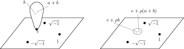
Figure 3. Universal family of deformation of $S^{2}$ with 3 marked points and one sphere bubble

Remark 3.25.

In the situation of Theorem 3.5 we consider a neighborhood of the image of $\mathcal{ID}:\mathcal{OB}\to\mathcal{MOR}$. Since ${\rm Pr}_{t}$ is a submersion we may identify this neighborhood with a direct product $\mathfrak{H}\times\mathcal{OB}$. We assign to $(\varphi,{\bf x})\in\mathfrak{H}\times\mathcal{OB}$ the element ${\rm Pr}_{s}(\varphi)$. We thus obtain a map

(3.20) $$\mathfrak{H}\times\mathcal{OB}\to\mathcal{OB}.$$

If $(\varphi,{\bf x})\in\mathfrak{H}\times\mathcal{OB}$ are sent to ${\bf y}$ then $\varphi$ induces an isomorphism between two marked nodal curves represented by ${\bf x}$ and by ${\bf y}$. The map (3.20) is nothing but the map $act$ appearing in [FOn, page 990]. Since the product decomposition $\mathfrak{H}\times\mathcal{OB}$ of the neighborhood of the image of $\mathcal{ID}$ is not canonical, this is not really an action as we mentioned in [FOn, page 990].

4. $\epsilon$-closeness and obstruction bundle

Let $((\Sigma,\vec{z}),u)$ be a stable map of genus $g$ with $\ell$ marked points in a symplectic manifold $(X,\omega)$ on which $G$ acts preserving $\omega$. See for example [FOn, Definition 7.4] for the definition of stable map. We take the universal family of deformations $\mathscr{G}=(\widetilde{\mathfrak{G}},\mathscr{F},{\mathfrak{G}},\vec{\mathfrak{T}},o,\iota)$ of $(\Sigma,\vec{z})$. We fix Riemannian metrics on the spaces of morphisms and objects of $\widetilde{\mathfrak{G}}$, ${\mathfrak{G}}$. We also choose a $G$-invariant Riemannian metric on $X$. We put

(4.1) $$\widehat{\mathcal{G}}_{c}=\left\{(\gamma,g)\,\,\left|\begin{aligned} &\gamma:(\Sigma,\vec{z})\to(\Sigma,\vec{z}),\text{$\gamma$ is bi-holomorphic},\\ &g\in G\quad u(\gamma x)=gu(x)\end{aligned}\right\}\right..$$

We define its group structure by

(4.2) $$(\gamma_{1},g_{1})\cdot(\gamma_{2},g_{2})=(\gamma_{1}\gamma_{2},g_{1}g_{2}).$$

We define a group homomorphism $\widehat{\mathcal{G}}_{c}\to\mathcal{G}$ by $(\gamma,g)\mapsto\gamma$ and denote by ${\mathcal{G}}_{c}$ the image. Note $\mathcal{G}$ is defined by (3.5). This is a compact subgroup of $\mathcal{G}$. Using Proposition 3.22 we may assume that $\mathscr{G}$ has $\mathcal{G}_{c}$ action in the sense stated in Proposition 3.22.

We will next fix a ‘trivialization’ of the ‘bundle’ $\mathscr{F}_{ob}:\widetilde{\mathcal{OB}}\to\mathcal{OB}$. Note this ‘bundle’ coincides with $\pi:\mathcal{C}\to\mathcal{V}$ using the notation we used during the proof of Theorem 3.5. We first recall that we take universal families $\mathcal{C}_{a}\to\mathcal{V}_{a}$ of deformations of $(\Sigma_{a},\vec{z}_{a})$ for each stable irreducible component $a\in\mathcal{A}_{s}$. They are fiber bundles. Therefore we obtain their $C^{\infty}$ trivialization by choosing $\mathcal{V}_{a}$ small. It gives a diffeomorphism

$$\phi_{a}:\mathcal{V}_{a}\times\Sigma_{a}\to\mathcal{C}_{a}$$

onto an open subset such that the next diagram commutes:

(4.3) $$\begin{CD}\mathcal{V}_{a}\times\Sigma_{a}@ >{\phi_{a}}>>\mathcal{C}_{a}\\ @ VVV@ VV{\pi}V\\ \mathcal{V}_{a}@ >{\rm id}>>\mathcal{V}_{a}.\end{CD}$$

We require the following properties:

1. $\phi_{a}$ is $\mathcal{G}_{a}$ equivariant.

2. $$(\phi_{a})^{-1}(\mathfrak{T}_{a,j}(x))=(x,z_{a,j}).$$

   Namely by this trivialization the sections $\mathfrak{T}_{a,j}$ becomes a constant map to $z_{a,j}$ (that is, the $j$-th marked point of $(\Sigma_{a},\vec{z}_{a})$).

3. Let $\varphi_{a,i}:\mathcal{V}_{a}\times D^{2}(2)\to\mathcal{C}_{a}$ be the analytic family of coordinates as in Definition 3.9. Then we have

   $$(\phi_{a})^{-1}(\varphi_{a,i}(x,z))=(x,\varphi_{a,i}(0,z)).$$

   Here $0\in\mathcal{V}_{a}$ corresponds to the point $\Sigma_{a}$.

4. Let $\mathscr{H}_{c}$ be as in (3.19). Then the next diagram commutes for $\gamma\in\mathscr{H}_{c}$. Note $\mathscr{H}_{c}$ acts on the dual graph of $\Sigma$. So for $a\in\mathcal{A}_{s}$ we obtain $\gamma a\in\mathcal{A}_{s}$.

   (4.4) $$\begin{CD}\mathcal{V}_{a}\times\Sigma_{a}@ >{\phi_{a}}>>\mathcal{C}_{a}\\ @ VV{\gamma}V@ VV{\gamma}V\\ \mathcal{V}_{\gamma a}\times\Sigma_{\gamma a}@ >{\Phi_{\gamma a}}>>\mathcal{C}_{\gamma a}.\end{CD}$$

Existence of such trivialization in $C^{\infty}$ category is standard. (It is nothing but the local smooth triviality of fiber bundles, which is a consequence of local contractibility of the group of diffeomorphisms.)

The above trivialization is defined on $\mathcal{V}_{0}\subset\mathcal{V}$. We extend it including the gluing parameter as follows.

Let $\delta>0$. We put

(4.5) $$\mathcal{V}_{1}(\delta)=\{(\rho_{\rm e})_{{\rm e}\in\Gamma(\Sigma)}\mid\forall{\rm e},|\rho_{\rm e}|<\delta\}.$$

Let ${\bf x}=((x_{a})_{a\in\mathcal{A}_{s}},(\rho_{\rm e})_{{\rm e}\in\Gamma(\Sigma)})\in\mathcal{V}_{0}\times\mathcal{V}_{1}(\delta)\subset\mathcal{OB}$. We put

(4.6) $$\Sigma({\bf x})=\mathscr{F}_{ob}^{-1}({\bf x})$$

(= $\pi^{-1}(\bf x)\subset\mathcal{C}$) and $\vec{z}({\bf x})=(\mathfrak{T}_{j}({\bf x}))_{j=1}^{\ell}$.

We also put

(4.7) $$\Sigma(\delta)=\bigcup_{a\in\mathcal{A}}(\Sigma_{a}\setminus\bigcup\varphi_{a,j}(D^{2}(\delta))),$$

where the union $\bigcup\varphi_{a,j}(D^{2}(\delta))$ is taken over all nodal points contained in $\Sigma_{a}$.

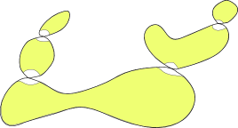
Figure 4. $\Sigma(\delta)$

We will construct a smooth embedding

(4.8) $$\Phi_{{\bf x},\delta}:\Sigma(\delta)\to\Sigma({\bf x})$$

below. Let $\Sigma_{a}(x_{a})=\pi^{-1}(x_{a})\subset\mathcal{C}_{a}$. We put

(4.9) $$\Sigma(\delta;(x_{a})_{a\in\mathcal{A}_{s}}))=\bigcup_{a\in\mathcal{A}}(\Sigma_{a}(x_{a})\setminus\bigcup\varphi_{a,j}(\{x_{a}\}\times D^{2}(\delta))),$$

The maps $\phi_{a}$ for $a\in\mathcal{A}_{s}$ define a diffeomorphism

$$\Phi_{((x_{a})_{a\in\mathcal{A}_{s}})}:\Sigma(\delta)\to\Sigma(\delta;(x_{a})_{a\in\mathcal{A}_{s}}).$$

(Note for an unstable component $\Sigma_{a}$ the corresponding component of $\Sigma(\delta;(x_{a})_{a\in\mathcal{A}_{s}})$ is identified with $\Sigma_{a}$ itself. In this case $\Phi_{{\bf x},\delta}$ on this component is the identity map.)

The $C^{\infty}$ embedding

$$\Sigma(\delta;(x_{a})_{a\in\mathcal{A}_{s}})\to\Sigma({\bf x})$$

is obtained by construction. (In fact $\Sigma({\bf x})$ is obtained by gluing $\Sigma_{a}(x_{a})\setminus\bigcup\varphi_{a,j}(\{x_{a}\}\times D^{2}(|\rho_{a}|))$.) Thus we obtain an open embedding of $C^{\infty}$ class

(4.10) $$\Phi_{\bf x,\delta}:\Sigma(\delta)\to\Sigma({\bf x})$$

by composing them.

Definition 4.1.

Let $F:A\to X$ be a continuous map from a topological space to a metric space. We say $F$ has diameter $<\epsilon$ on $A$ if for each connected component $A_{a}$ of $A$ the diameter of $F(A_{a})$ is smaller than $\epsilon$.

Definition 4.2.

We consider a triple $((\Sigma^{\prime},\vec{z}^{\,\prime}),u^{\prime})$ where $(\Sigma^{\prime},\vec{z}^{\,\prime})$ is a nodal curve of genus $g$ with $\ell$ marked points, $u^{\prime}:\Sigma^{\prime}\to X$ is a smooth map.

We say that $((\Sigma^{\prime},\vec{z}^{\,\prime}),u^{\prime})$ is $G$-$\epsilon$-close to $((\Sigma,\vec{z}),u)$ if there exist $g\in G$, $\delta>0$, ${\bf x}=((x_{a})_{a\in\mathcal{A}_{s}},(\rho_{\rm e})_{{\rm e}\in\Gamma(\Sigma)})\in\mathcal{V}_{0}\times\mathcal{V}_{1}(\delta)\subset\mathcal{OB}$, and a bi-holomorphic map $\phi:(\Sigma({\bf x}),\vec{z}({\bf x}))\cong(\Sigma^{\prime},\vec{z}^{\,\prime})$ with the following properties.

1. The $C^{2}$ difference between $u^{\prime}\circ\phi\circ\Phi_{\bf x,\delta}$ and $g\circ u|_{\Sigma(\delta)}$ is smaller than $\epsilon$.

2. The distance between $\bf x$ and $o\in\mathcal{OB}$ is smaller than $\epsilon$. Moreover $\delta<\epsilon$.

3. The map $u^{\prime}\circ\phi$ has diameter $<\epsilon$ on $\Sigma({\bf x})\setminus{\rm Image}(\Phi_{\bf x,\delta})$.

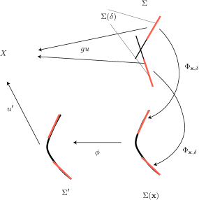
Figure 5. $((\Sigma^{\prime},\vec{z}^{\,\prime}),u^{\prime})$ is $G$-$\epsilon$-close to $((\Sigma,\vec{z}),u)$

In case we need to specify $g$, $\bf x$, $\phi$ we say $((\Sigma^{\prime},\vec{z}^{\,\prime}),u^{\prime})$ is $G$-$\epsilon$-close to $((\Sigma,\vec{z}),u)$ by $g$, $\bf x$, $\phi$.

We say that $((\Sigma^{\prime},\vec{z}^{\,\prime}),u^{\prime})$ is $\epsilon$-close to $((\Sigma,\vec{z}),u)$ if (2),(3) are satisfied and (1) is satisfied with $g=1$. In case we need to specify $\bf x$, $\phi$ we say $((\Sigma^{\prime},\vec{z}^{\,\prime}),u^{\prime})$ is $\epsilon$-close to $((\Sigma,\vec{z}),u)$ by $\bf x$, $\phi$.

The main part of the construction of our Kuranishi chart is to associate a finite dimensional subspace

$$E((\Sigma^{\prime},\vec{z}^{\,\prime}),u^{\prime})\subset C^{\infty}(\Sigma({\bf x});(u^{\prime})^{*}TX\otimes\Lambda^{01})$$

to each $((\Sigma^{\prime},\vec{z}^{\,\prime}),u^{\prime})$ which is $G$-$\epsilon$-close to $((\Sigma,\vec{z}),u)$ such that

$$E((\Sigma^{\prime},\vec{z}^{\,\prime}),gu^{\prime})=g_{*}E((\Sigma^{\prime},\vec{z}^{\,\prime}),u^{\prime})$$

holds for $g\in G$.

The construction of such $E((\Sigma^{\prime},\vec{z}^{\,\prime}),u^{\prime})$ will be completed in Section 6 using center of mass technique which we review in Section 8.

Definition 4.3.

We say a subspace

$$E((\Sigma,\vec{z}),u)\subset C^{\infty}(\Sigma({\bf x});u^{*}TX\otimes\Lambda^{01})$$

an obstruction space at origin if the following is satisfied.

1. $E((\Sigma,\vec{z}),u)$ is a finite dimensional linear subspace.

2. The support of each element of $E((\Sigma,\vec{z}),u)$ is contained in the complement of the image of $\varphi_{a,i}:D^{2}(2)\to\Sigma_{a}$ for all $a$ and $i$ corresponding to a nodal point.

3. $E((\Sigma,\vec{z}),u)$ is invariant under the $\widehat{\mathcal{G}}_{c}$ action, which we explain below.

4. $E((\Sigma,\vec{z}),u)$ satisfies the transversality condition, Condition 4.6 below.

We define $\widehat{\mathcal{G}}_{c}$ action on $C^{\infty}(\Sigma({\bf x});u^{*}TX\otimes\Lambda^{01})$. Let $(\gamma,g)\in\widehat{\mathcal{G}}_{c}$ be as in (4.1) and $v\in C^{\infty}(\Sigma({\bf x});u^{*}TX\otimes\Lambda^{01})$. Using the differential of $g$ we have

$$g_{*}v\in C^{\infty}(\Sigma({\bf x});(g\circ u)^{*}TX\otimes\Lambda^{01}).$$

Since $g\circ u=u\circ\gamma$ we may regard

$$g_{*}v\in C^{\infty}(\Sigma({\bf x});(u\circ\gamma)^{*}TX\otimes\Lambda^{01}).$$

Since $\gamma:\Sigma\to\Sigma$ is bi-holomorphic we have

$$(g,\gamma)_{*}v\in C^{\infty}(\Sigma({\bf x});u^{*}TX\otimes\Lambda^{01}).$$

We thus defined $\widehat{\mathcal{G}}_{c}$ action on $C^{\infty}(\Sigma({\bf x});u^{*}TX\otimes\Lambda^{01})$. Item (3) above requires that the subspace $E((\Sigma,\vec{z}),u)$ is invariant under this action.

We next define transversality conditions in Item (4). We decompose $\Sigma$ into irreducible components $\Sigma_{a}$ ($a\in\mathcal{A}$). We consider

$$L^{2}_{m+1}(\Sigma_{a};u^{*}TX)$$

the Hilbert space of sections of $u^{*}TX$ of $L^{2}_{m+1}$ class on $\Sigma_{a}$. (We take $m$ sufficiently large and fix it.) For each $z_{a,j}$ we have an evaluation map:

$${\rm Ev}_{z_{a,j}}:L^{2}_{m+1}(\Sigma_{a};u^{*}TX)\to T_{u(z_{a,j})}X.$$

(Since $m$ is large elements of $L^{2}_{m+1}(\Sigma_{a};u^{*}TX)$ are continuous and ${\rm Ev}_{z_{a,j}}$ is well-defined and continuous.)

Definition 4.4.

The Hilbert space

$$W^{2}_{m+1}(\Sigma;u^{*}TX)$$

is the subspace of the direct sum

(4.11) $$\bigoplus_{a\in\mathcal{A}}L^{2}_{m+1}(\Sigma_{a};u^{*}TX)$$

consisting of elements $(v_{a})_{a\in\mathcal{A}}$ such that the following holds.

For each edge ${\rm e}$ of $\Gamma(\Sigma)$, that corresponds to the nodal points, let $z_{-,{\rm e}},z_{+,{\rm e}}\in{\rm Node}$ such that the orientation of ${\rm e}$ goes from the vertex corresponding to $z_{-,{\rm e}}$ to the vertex corresponding to $z_{+,{\rm e}}$. Let $a({\rm e},-)$ and $a({\rm e},+)$ be the irreducible components containing $z_{-,{\rm e}}$, $z_{+,{\rm e}}$, respectively. We then require

(4.12) $${\rm Ev}_{z_{-,{\rm e}}}(v_{a({\rm e},-)})={\rm Ev}_{z_{+,{\rm e}}}(v_{a({\rm e},+)}).$$

Note $\vec{z}$ (the set of marked points of $\Sigma$) is a subset of $\bigcup_{a\in\mathcal{A}}\vec{z}_{a}$. Therefore we obtain an evaluation maps

(4.13) $${\rm Ev}_{z_{i}}:W^{2}_{m+1}(\Sigma;u^{*}TX)\to T_{u(z_{i})}X.$$

We put

$$L^{2}_{m}(\Sigma;u^{*}TX\otimes\Lambda^{01})=\bigoplus_{a\in\mathcal{A}}L^{2}_{m}(\Sigma_{a};u^{*}TX\otimes\Lambda^{01})$$

The linearization of the equation $\overline{\partial}u=0$ defines a linear differential operator of first order:

(4.14) $$D_{u}\overline{\partial}:W^{2}_{m+1}(\Sigma;u^{*}TX)\to L^{2}_{m}(\Sigma;u^{*}TX\otimes\Lambda^{01}).$$

It is well-known that (4.14) is a Fredholm operator.

In fact the operator

(4.15) $$D_{u_{a}}\overline{\partial}:L^{2}_{m+1}(\Sigma_{a};{u_{a}}^{*}TX)\to L^{2}_{m}(\Sigma_{a};{u_{a}}^{*}TX\otimes\Lambda^{01})$$

is Fredholm by ellipticity. The source of (4.14) is a space of finite codimension of the direct sum of the sources of (4.15).

Remark 4.5.

In Definition 4.4 we considered the compact spaces (manifold) $\Sigma_{a}$. Instead we may take $\Sigma_{a}\setminus\vec{z}_{a}$ and put cylindrical metric (which is isometric to $S^{1}\times[0,\infty)$ at the neighborhood of each nodal points), and use appropriate weighted Sobolev-norm. (See [FOOO8, Section 4] for example.) The resulting transversality conditions are equivalent to one in Condition 4.6.

Condition 4.6.

We require the next two transversality conditions.

1. The sum of the image of the operator $D_{u}\overline{\partial}$ (4.14) and the subspace $E((\Sigma,\vec{z}),u)$ is $L^{2}_{m}(\Sigma;u^{*}TX\otimes\Lambda^{01})$.

2. We consider

   $${\rm Ker}^{+}D_{u}\overline{\partial}=\{v\in W^{2}_{m+1}(\Sigma;u^{*}TX)\mid D_{u}\overline{\partial}(v)\in E((\Sigma,\vec{z}),u).\}$$

   Then the restriction of ${\rm Ev}_{z_{i}}$ defines a surjective map

   (4.16) $$\bigoplus_{i=1}^{\ell}{\rm Ev}_{z_{i}}:{\rm Ker}^{+}D_{u}\overline{\partial}\to\bigoplus_{i=1}^{\ell}T_{u(z_{i})}X.$$

Remark 4.7.

In certain situation we relax the condition (2) and require surjectivity of one of ${\rm Ev}_{z_{i}}$ only. (See [Fu1].)

Proposition 4.8.

There exists an obstruction space at origin as in Definition 4.3.

Proof.

This is mostly obvious using Fredholm property of $D_{u}\overline{\partial}$ and the unique continuation. See [FOOO4, Lemma 4.3.5] for example. ∎

5. Definition of $G$-equivariant Kuranishi chart and the statement of the main theorem

We review the notion of $G$-equivariant Kuranishi chart. In the case of finite group $G$ it is defined for example in [FOOO9, Definition 7.5]. The notion of $S^{1}$ equivariant Kuranishi structure is in [FOOO6, Definition 28.1]. In fact we studied in [FOOO6, Definition 28.1] the $S^{1}$ action on the moduli space induced by the $S^{1}$ action of the source curve. Such an $S^{1}$ action is much easier to handle than the target space action we are studying here. (This $S^{1}$ action had been used in the study of periodic Hamiltonian system and thorough detail of its construction and of its usage had been written in [FOOO6, Part 5].)

We first review the notion of group action on effective orbifolds. For the definition of effective orbifolds and its morphisms etc. using coordinate we refer the reader to [FOOO11, Section 15], [FOOO5, Part 7] or [FOOO14, Section 23].

An orbifold $M$ is a paracompact and Hausdorff topological space together with a system of local charts $(V,\Gamma,\phi)$, where $V$ is a manifold, $\Gamma$ is a finite group which acts on $V$ effectively and $\phi:V\to M$ is a smooth map which induces a homeomorphism $V/\Gamma\to M$ onto an open neighborhood of $p$ in $M$. When $M$ is covered by the images of several local charts $(V_{i},\Gamma_{i},\phi_{i})$ satisfying certain compatibility conditions (see [FOOO11, Section 15], [FOOO5, Part 7] or [FOOO14, Section 23], they give an orbifold structure of $M$. An orbifold structure is the set of all charts $(V,\Gamma,\phi)$ which are compatible with the given charts.

Let $M_{1},M_{2}$ be orbifolds. A topological embedding $f:M_{1}\to M_{2}$ is said to be an orbifold embedding if for each $p\in M_{1}$ we can take a chart $(V_{1},\Gamma_{1},\phi_{1})$ of $p$ in $M_{1}$, $(V_{2},\Gamma_{2},\phi_{2})$ of $f(p)$ in $M_{2}$ and $f_{p}:V_{1}\to V_{2}$, $h_{p}:\Gamma_{1}\to\Gamma_{2}$ such that:

1. $f_{p}$ is a smooth embedding of manifolds.

2. $h_{p}$ is an isomorphism of groups.

3. $f_{p}(gx)=h_{p}(g)f_{p}(x)$.

4. $\phi_{2}\circ f_{p}=f\circ\phi_{1}$.

Note two orbifold embeddings are regarded as the same if they coincide set theoretically. (In other words, the existence of $f_{p},h_{p}$ above is the condition for $f$ to be an orbifold embedding and is not a part of the data consisting of an orbifold embedding.)

A homeomorphism between orbifolds is said to be a diffeomorphism if it is an embedding of orbifold.

The set of all diffeomorphisms of an orbifold $M$ becomes a group which we write ${\rm Diff}(M)$. The group ${\rm Diff}(M)$ becomes a topological group by compact open topology.

Definition 5.1.

Let $G$ be a Lie group. A smooth action of $G$ on $M$ is by definition a continuous group homomorphism $G\to{\rm Diff}(M)$ with the following properties. Note $G\to{\rm Diff}(M)$ induces a continuous map $G\times M\to M$.

For each $p\in M$ and $g\in G$ there exists a chart $(V_{1},\Gamma_{1},\phi_{1})$ of $p$, a chart $(V_{2},\Gamma_{2},\phi_{2})$ of $gp$, an open neighborhood $U$ of $g$, and maps $f_{p,g}:U\times V_{1}\to V_{2}$, $h_{p,g}:\Gamma_{1}\to\Gamma_{2}$ such that:

1. $f_{p,g}$ is a smooth map.

2. $h_{p,g}$ is a group isomorphism.

3. $f_{p,g}$ is $h_{p,g}$ equivariant.

4. $\phi_{2}(gv)=g\phi_{1}(v)$.

A (smooth) vector bundle $\mathcal{E}\to M$ on an orbifold is a pair of orbifolds $\mathcal{E}$, $M$ and a continuous map $\pi:\mathcal{E}\to M$ such that for each $\tilde{p}\in\mathcal{E}$ we can take a special choice of coordinates of $\tilde{p}$ and $\pi(p)$ as follows. $(V,\Gamma,\phi)$ is a coordinate of $M$ at $p$. $(V\times E,\Gamma,\tilde{\phi})$ is a coordinate of $\mathcal{E}$ at $\tilde{p}$, where $E$ is a vector space on which $G$ has a linear action. Moreover the next diagram commutes,

(5.1) $$\begin{CD}V\times E@ >{\tilde{\phi}}>>\mathcal{E}\\ @ VVV@ VV{\pi}V\\ V@ >{\phi}>>M,\end{CD}$$

where the first vertical arrow is the obvious projection. See [FOOO11, Definition 15.7 (3)], [FOOO5, Definition 31.3] or [FOOO14, Definition 23.19] for the condition required to the coordinate change.

Suppose $M$ has a $G$-action. A $G$-action on a vector bundle $\mathcal{E}\to M$ is by definition a $G$-action on $\mathcal{E}$ such that the projection $\mathcal{E}\to M$ is $G$-equivariant, (Here $G$-equivariance means that $\pi(g\tilde{p})=g\pi(\tilde{p})$, set theoretically.) and that the local expression

$$f_{p,g}:G\times(V_{1}\times E_{1})\to V_{2}\times E_{2}$$

of $G$ action preserves the structure of vector space of $E_{1}$, $E_{2}$. Namely for each $g\in G$, $v\in V_{1}$ the map

$$V\mapsto\pi_{E_{2}}(f(g,v,V)),E_{1}\to E_{2}$$

is linear. (Here $\pi_{E_{2}}:V_{2}\times E_{2}\to E_{2}$ is the projection.)

If $\mathcal{E}\to M$ is a vector bundle on an orbifold, its section is by definition an orbifold embedding $s:M\to\mathcal{E}$ such that the composition $M\to\mathcal{E}\to M$ is the identity map (set theoretically). If $s$ is a section then $(gs)(p)=g(s(g^{-1}p))$ defines a section $gs:M\to\mathcal{E}$. We say $s$ is $G$-equivariant if $gs=s$. If $s$ is a $G$-equivariant section then

$$s^{-1}(0)=\{x\in M\mid s(x)=0\}$$

is $G$-invariant subset of $M$. (Here $0\subset\mathcal{E}$ is the set such that by the coordinate $(V\times E,\Gamma,\tilde{\phi})$ it corresponds to a point in $V\times\{0\}$.)

Now we define the notion of $G$-equivariant Kuranishi chart as follows.

Definition 5.2.

Let $X$ be a metrizable space on which a compact Lie group $G$ acts and $p\in X$. A $G$-equivariant Kuranishi chart of $X$ at $p$ is an object $(U,\mathcal{E},s,\psi)$ such that:

1. We are given an orbifold $U$, on which $G$ acts.

2. We are given a $G$-equivariant vector bundle $\mathcal{E}$ on $U$.

3. We are given a $G$-equivariant smooth section $s$ of $\mathcal{E}$.

4. We are given a $G$-equivariant homeomorphism $\psi:s^{-1}(0)\to X$ onto an open set.

We call $U$ the Kuranishi neighborhood, $\mathcal{E}$ the obstruction bundle, $s$ the Kuranishi map, and $\psi$ the parametrization.

Let $(X,\omega)$ be a compact symplectic manifold on which a compact Lie group $G$ acts preserving the symplectic structure $\omega$. We define an equivalence relation on $\pi_{2}(X)$ by

$$[v]\sim[v^{\prime}]\quad\Leftrightarrow\qquad\int v^{*}\omega=\int(v^{\prime})^{*}\omega,\quad v_{*}([S^{2}])\cap c^{1}(X)=v^{\prime}_{*}([S^{2}])\cap c^{1}(X).$$

We denote by $\Pi_{2}(X)$ the group of the equivalence classes of $\sim$. Let $\alpha\in\Pi_{2}(X)$ and $g,\ell$ be nonnegative integers. We take and fix a $G$-invariant compatible almost complex structure $J$ on $X$. Let $\mathcal{M}_{g,\ell}((X,J);\alpha)$ be the moduli space of $J$-holomorphic stable maps of genus $g$ with $\ell$ marked points and homology class is $\alpha$. See for example [FOn, Defnition 7.7] for its definition. (The notion of stable map is introduced by Kontsevitch. Systematic study of the moduli space $\mathcal{M}_{g,\ell}((X,J);\alpha)$ in the semi-positive case was initiated by Ruan-Tian [RT1] [RT2]. Studying $J$-holomorphic curve in symplectic geometry is a great invention by Gromov. There is a nice account of genus zero case by McDuff-Salamon [MS].) The topology (stable map topology) on $\mathcal{M}_{g,\ell}((X,J);\alpha)$ was introduced by Fukaya-Ono (in the year 1996) in [FOn, Defnition 10.3] and they proved that $\mathcal{M}_{g,\ell}((X,J);\alpha)$ is compact ([FOn, Theorem 11.1]) and Hausdorff ([FOn, Lemma 10.4]), in this particular topology. There exist evaluation maps ${\rm ev}:\mathcal{M}_{g,\ell}((X,J);\alpha)\to X^{\ell}$. (See [FOn, page 936, line 3].)

Since $J$ is $G$-equivariant it is easy to see that the group $G$ acts on the topological space $\mathcal{M}_{g,\ell}((X,J);\alpha)$.

Now the main result of this paper is the following:

Theorem 5.3.

For each $p\in\mathcal{M}_{g,\ell}((X,J);\alpha)$, there exists a $G$-equivariant Kuranishi chart of $\mathcal{M}_{g,\ell}((X,J);\alpha)$ at $p$.

The evaluation map ${\rm ev}:\mathcal{M}_{g,\ell}((X,J);\alpha)\to X^{\ell}$ is an underlying continuous map of a weakly submersive map.

Remark 5.4.

Note since the parametrization $\psi$ is assumed to be $G$-equivariant its image necessary contains the $G$-orbit of $p$ in $\mathcal{M}_{g,\ell}((X,J);\alpha)$. Therefore a $G$-equivariant Kuranishi chart cannot be completely local in $\mathcal{M}_{g,\ell}((X,J);\alpha)$.

Remark 5.5.

Once we proved Theorem 5.3 we can construct a $G$-equivariant Kuranishi structure on $\mathcal{M}_{g,\ell}((X,J);\alpha)$ in the same way as the case without $G$ action. (See for example [FOOO12], [FOOO13].) In this paper we focus on proving Theorem 5.3 since this is the novel part in our $G$-equivariant situation.

6. Proof of the main theorem

In this section we prove Theorem 5.3 except a few points postponed to later sections. Let $((\Sigma^{\prime},\vec{z}^{\,\prime}),u^{\prime})$ be an object which is G-$\epsilon_{1}$-close to $((\Sigma,\vec{z}),u)$. (We determine the positive constant $\epsilon_{1}$ later.) We fix ${\bf x}_{0}\in\mathcal{OB}$ such that $(\Sigma^{\prime},\vec{z}^{\,\prime})$ is bi-holomorphic to $(\Sigma({\bf x}_{0}),\vec{z}({\bf x}_{0}))$. We also fix a bi-holomorphic map $\phi_{0}:(\Sigma({\bf x}_{0}),\vec{z}({\bf x}_{0}))\cong(\Sigma^{\prime},\vec{z}^{\,\prime})$.

Definition 6.1.

We define $\mathcal{W}(\epsilon_{1};{\bf x}_{0},\phi_{0};((\Sigma^{\prime},\vec{z}^{\,\prime}),u^{\prime}))$ as the set of pairs $(\varphi,g)$ such that:

1. $\varphi\in\mathcal{MOR}$, $g\in G$.

2. ${\rm Pr}_{t}(\varphi)={\bf x}_{0}$.

3. We put ${\bf x}^{\prime}={\rm Pr}_{s}(\varphi)$. The morphism $\varphi$ defines a bi-holomorphic map

   $$\varphi:(\Sigma({\bf x}^{\prime}),\vec{z}({\bf x}^{\prime}))\cong(\Sigma({\bf x}_{0}),\vec{z}({\bf x}_{0})).$$

   We consider $\phi_{0}\circ\varphi:(\Sigma({\bf x}^{\prime}),\vec{z}({\bf x}^{\prime}))\to(\Sigma^{\prime},\vec{z}^{\,\prime})$. Then $((\Sigma^{\prime},\vec{z}^{\,\prime}),u^{\prime})$ is $2\epsilon_{1}$- close to $((\Sigma,\vec{z}),gu)$ by ${\bf x}^{\prime}$, $\phi_{0}\circ\varphi$.

Lemma 6.2.

The space $\mathcal{W}(\epsilon_{1};{\bf x}_{0},\phi_{0};((\Sigma^{\prime},\vec{z}^{\,\prime}),u^{\prime}))$ has a structure of smooth manifold.

Proof.

The set of $(\varphi,g)$ satisfying Items (1)(2) has a structure of smooth manifold since $\mathcal{MOR}$ is a smooth manifold and ${\rm Pr}_{t}$ is a submersion. Since the condition (3) is an open condition the space $\mathcal{W}(\epsilon_{1};{\bf x}_{0},\phi_{0};((\Sigma^{\prime},\vec{z}^{\,\prime}),u^{\prime}))$ is an open set of a smooth manifold and so has a structure of smooth manifold. ∎

We used ${\bf x}_{0},\phi_{0}$ to define $\mathcal{W}(\epsilon_{1};{\bf x}_{0},\phi_{0};((\Sigma^{\prime},\vec{z}^{\,\prime}),u^{\prime}))$. However this manifold is independent of the choice of such ${\bf x}_{0},\phi_{0}$ as the next lemma shows.

Lemma 6.3.

Let ${\bf x}_{1}\in\mathcal{OB}$ and $\phi_{1}:(\Sigma({\bf x}_{1}),\vec{z}({\bf x}_{1}))\cong(\Sigma^{\prime},\vec{z}^{\,\prime})$ be a bi-holomorphic map.

The composition $\phi_{1}^{-1}\circ\phi_{0}$ determines an element $\psi\in\mathcal{MOR}$ such that ${\rm Pr}_{s}(\psi)={\rm Pr}_{t}(\psi)={\bf x}_{1}$.

Then the next two conditions are equivalent.

1. $(\varphi,g)\in\mathcal{W}(\epsilon_{1};{\bf x}_{0},\phi_{0};((\Sigma^{\prime},\vec{z}^{\,\prime}),u^{\prime}))$.

2. $(\psi\circ\varphi,g)\in\mathcal{W}(\epsilon_{1};{\bf x}_{1},\phi_{1};((\Sigma^{\prime},\vec{z}^{\,\prime}),u^{\prime}))$.

The proof of Lemma 6.3 are obvious from definition.

Definition 6.4.

Let $\sigma$ be a positive number which we will fix during the proof of Lemma 6.6. We take a smooth function $\chi:\Sigma_{0}(\sigma)\to[0,1]$ such that:

1. $\chi\equiv 1$ on $\Sigma_{0}(2\sigma)$.

2. $\chi$ has compact support.

3. $\chi$ is $\mathcal{G}_{c}$ invariant. Here $\mathcal{G}_{c}$ is defined by (4.1).

Definition 6.5.

We define a function ${\rm meandist}:\mathcal{W}(\epsilon_{1};{\bf x}_{0},\phi_{0};((\Sigma^{\prime},\vec{z}^{\,\prime}),u^{\prime}))\to{\mathbb{R}}$ as follows.

(6.1) $${\rm meandist}(\varphi,g)=\int_{z\in\Sigma(\sigma)}\chi(z)\,\,d_{X}^{2}((u^{\prime}\circ\phi_{0}\circ\varphi\circ\Phi_{{\bf x}^{\prime},\sigma})(z),gu(z)\,\,\Omega_{\Sigma}.$$

Here $\Omega_{\Sigma}$ is the volume element of $\Sigma$ and $d_{X}$ is the Riemannian distance function on $X$. We assume $\Omega_{\Sigma}$ is invariant under ${\mathcal{G}}_{c}$ action.

The main properties of this function is given below.

Lemma 6.6.

The function ${\rm meandist}$ has the following properties if $\epsilon_{1}$ is sufficiently small.

1. ${\rm meandist}$ is a convex function.

2. If $\mathcal{W}(\epsilon_{1};{\bf x}_{0},\phi_{0};((\Sigma^{\prime},\vec{z}^{\,\prime}),u^{\prime}))\cong\mathcal{W}(\epsilon_{1};{\bf x}_{1},\phi_{1};((\Sigma^{\prime},\vec{z}^{\,\prime}),u^{\prime}))$ is the isomorphism given in Lemma 6.3 then ${\rm meandist}$ is compatible with this isomorphism.

Proof.

(2) is obvious from construction. The convexity of ${\rm meandist}$ follows from the convexity of distance function. (We omit the detail of the proof of convexity here since we will prove a stronger result in Proposition 6.8.) ∎

The function ${\rm meandist}$ is not in general strictly convex. To obtain strictly convex function we need to take the quotient by the $\widehat{\mathcal{G}}_{c}$ action as follows. For each $\upsilon=(\gamma,h)\in\hat{\mathcal{G}}_{c}$ and ${\bf x}\in\mathcal{OB}$ we have $\gamma{\bf x}\in\mathcal{OB}$ and a bi-holomorphic map $\gamma_{*}:(\Sigma({\bf x}),\vec{z}({\bf x}))\to(\Sigma(\gamma{\bf x}),\vec{z}(\gamma{\bf x}))$. This is a consequence of Proposition 3.22. (We write $\gamma{\bf x}$ and $\gamma_{*}$ since it is independent of $h$.) By definition

(6.2) $$u\circ\gamma_{*}=h\circ u$$

where we consider the case ${\bf x}=0$, that is, $\gamma_{*}:(\Sigma,\vec{z})\to(\Sigma,\vec{z})$.

Definition 6.7.

We define a right $\widehat{\mathcal{G}}_{c}$ action on $\mathcal{W}(\epsilon_{1};{\bf x}_{0},\phi_{0};((\Sigma^{\prime},\vec{z}^{\,\prime}),u^{\prime}))$ as follows. Let $(\varphi,g)\in\mathcal{W}(\epsilon_{1};{\bf x}_{0},\phi_{0};((\Sigma^{\prime},\vec{z}^{\,\prime}),u^{\prime}))$. Let $\upsilon=(\gamma,h)\in\widehat{\mathcal{G}}_{c}$. We have ${\rm Pr}_{s}(\varphi)={\bf x}$. Set $\gamma^{-1}{\bf x}={\bf y}$ and $\gamma_{*}:(\Sigma({\bf y}),\vec{z}({\bf y}))\cong(\Sigma({\bf x}),\vec{z}({\bf x}))$. We may thus regard $\gamma_{*}\in\mathcal{MOR}$ with ${\rm Pr}_{s}(\gamma_{*})={\bf y}$ and ${\rm Pr}_{t}(\gamma_{*})={\bf x}$.

We now put

(6.3) $$\upsilon(\varphi,g)=(\varphi\circ\gamma_{*},gh).$$

It is easy to see that (6.3) defines a right $\widehat{\mathcal{G}}_{c}$ action on $\mathcal{W}(\epsilon_{1};{\bf x}_{0},\phi_{0};((\Sigma^{\prime},\vec{z}^{\,\prime}),u^{\prime}))$. We also observe that this action is free. In fact, if $(\gamma,e)\in\hat{\mathcal{G}}_{c}$ is not the unit then $\varphi\circ\gamma_{*}\neq\varphi$. (Here $e$ is the unit of $G$.)

Proposition 6.8.

For $\upsilon\in\hat{\mathcal{G}}_{c}$ we have

$${\rm meandist}(\upsilon(\varphi,g))={\rm meandist}(\varphi,g).$$

Moreover the induced function

$$\overline{\rm meandist}:\mathcal{W}(\epsilon_{1};{\bf x}_{0},\phi_{0};((\Sigma^{\prime},\vec{z}^{\,\prime}),u^{\prime}))/\widehat{\mathcal{G}}_{c}\to{\mathbb{R}}$$

is strictly convex if $\epsilon_{1}$ is sufficiently small.

Proof.

The first half follows from

$$d_{X}((u^{\prime}\circ\phi_{0}\circ\varphi\circ\gamma_{*})(z),ghu(z))=d_{X}((u^{\prime}\circ\phi_{0}\circ\varphi)(w),gu(w))$$

where $(\gamma_{*})(z)=w$. (Note $\Phi_{{\bf x},\sigma}^{-1}\circ\gamma_{*}\circ\Phi_{{\bf y},\sigma}:\Sigma(\sigma)\to\Sigma(\sigma)$ preserves $\Omega_{\Sigma}$ since it coincides with the action of $\gamma\in{\mathcal{G}}_{c}$.)

We next prove the strict convexity. Since $C^{2}$ difference between $u^{\prime}\circ\phi_{0}\circ\varphi\circ\Phi_{\bf x,\delta}$ and $g\circ u|_{\Sigma(\delta)}$ is smaller than $\epsilon$ and the strict convexity is preserved by a small $C^{2}$ perturbation, it suffices to show the case of $((\Sigma^{\prime},\vec{z}^{\,\prime}),u^{\prime})=((\Sigma,\vec{z}),u)$.

Let $t\mapsto(\varphi^{t},h^{t})$ be a geodesic of unit speed in the manifold $\mathcal{W}(\epsilon_{1};o,{\rm id};((\Sigma,\vec{z}),u))$, which is perpendicular to the $\widehat{\mathcal{G}}_{c}$ orbits at $t=0$. We will prove

(6.4) $$\frac{d^{2}}{dt^{2}}{\rm meandist}(\varphi^{t},h^{t})\geq\tau>0.$$

Note that $dh_{t}/dt|_{t=0}$ can be regarded as a vector field on $X$, which we denote by $V_{h}$. We consider the following 3 cases separately.

(Case 1) We first assume that there exists $z\in\Sigma$ such that

$$V_{h}(u(z))\notin D_{z}u(T_{z}{\Sigma}).$$

Note that the set of such points $z$ is open. Therefore we may choose $\sigma$ in Definition 6.4 so that we may assume $z\in\Sigma(\sigma)\cap\Sigma_{a}$. Then

(6.5) $$\int_{\Sigma_{a}\cap\Sigma(\sigma)}\chi(z)\,\,\left\|\frac{d}{dt}u(\varphi^{t}_{a}(z))-\frac{dh^{t}}{dt}u(z)\right\|^{2}\Omega_{\Sigma}\geq\rho.$$

at $t=0$, where $\rho>0$ is independent of $\epsilon_{1}$. Therefore Proposition 8.8 implies (6.4) at $t=0$. Since the third derivative of ${\rm meandist}$ is uniformly bounded we can choose $\epsilon_{1}$ small to conclude the required strict convexity.

(Case 2) We next assume $V_{h}(u(z))\in D_{z}u(T_{z}{\Sigma})$ for all $z\in\Sigma$. We also assume that $V_{h}(u(z))=0$ for all the nodal point $z$.

If $D_{z}u=0$ this implies that $V_{h}(u(z))=0$. If $D_{z}u\neq 0$ then $u$ is an immersion at $z$. Therefore there exists a unique $\tilde{V}_{h}(z)\in T_{z}\Sigma$ such that $V_{h}(u(z))=D_{z}u(\tilde{V}_{h}(z))$. Putting $\tilde{V}_{h}(z)=0$ when $D_{z}u=0$, we obtain a vector field $\tilde{V}_{h}$ of $C^{0}$ class on each $\Sigma_{a}$. The vector field $\tilde{V}_{h}$ is smooth on the open subset where $u$ is an immersion. Note that $G$ action preserves almost complex structure and $u$ is pseudo-holomorphic. We use this fact to show that $\tilde{V}_{h}$ is a holomorphic vector field (and in particular is of $C^{\infty}$ class) as follows. Let $K$ be a compact subset of the set of $z$ with $D_{z}u\neq 0$. It is easy to show that we can integrate $\tilde{V}_{h}$ to obtain a family of embeddings $\psi_{t}$ of a neighborhood of $K$ to $\Sigma$ for small $t$ such that

$$u\circ\psi_{t}={\rm Exp}(V_{h})\circ u.$$

Here we regard $V_{h}$ as an element of the Lie algebra of $G$. Since ${\rm Exp}(V_{h})\in G$ preserves almost complex structure $\psi_{t}$ is a holomorphic embedding. Therefore $\tilde{V}_{h}$ is a holomorphic vector field on $K$. Since $K$ is an arbitrary compact subset of the set of $z$ with $D_{z}u\neq 0$, $\tilde{V}_{h}$ is a holomorphic vector field outside its zero set. Therefore by Riemann’s removable singularity theorem $\tilde{V}_{h}$ is a holomorphic vector field on each $\Sigma_{a}$.

By assumption $\tilde{V}_{h}$ vanishes at each nodal points.

Thus $(\tilde{V}_{h},V_{h})$ is an element of the Lie algebra of $\widehat{\mathcal{G}}_{c}$. On the other hand, by assumption $\frac{d}{dt}(\varphi^{t},h^{t})|_{t=0}$ is perpendicular to a $\widehat{\mathcal{G}}_{c}$-orbit. Therefore there exists $\Sigma_{a}$ such that

(6.6) $$\int_{\Sigma_{a}\cap\Sigma(\sigma)}\chi(z)\,\,\left\|\frac{d\varphi^{t}}{dt}(0)-\tilde{V}_{h}(z)\right\|^{2}\Omega_{\Sigma}\geq\rho.$$

Since $V_{h}(u(z))=D_{z}u(\tilde{V}_{h}(z))$ it implies (6.5) at $t=0$. The rest of the proof is the same as (Case 1).

(Case 3) We finally consider the case when $V_{h}(u(z))$ is non-zero at certain nodal point $z$. Since strict convexity is an open property, we use (Case 2) and can assume that $\|V_{h}(u(z))\|\geq c_{0}$ for some positive constant $c_{0}$.

Note $\frac{d}{dt}u(\varphi^{t}_{a}(z))$ is zero at the nodal point $z$. Therefore we can choose $\sigma$ small such that (6.5) holds at $t=0$. The rest of the proof is the same as (Case 1).

The proof of Proposition 6.8 is complete. ∎

Lemma 6.9.

If $\epsilon_{1}$ is enough small then $\overline{\rm meandist}$ attains its local minimum at a unique point of $\mathcal{W}(\epsilon_{1};{\bf x}_{0},\phi_{0};((\Sigma^{\prime},\vec{z}^{\,\prime}),u^{\prime}))/\widehat{\mathcal{G}}_{c}$.

Proof.

In case $((\Sigma^{\prime},\vec{z}^{\,\prime}),u^{\prime})=((\Sigma,\vec{z}),gu)$ the local minimum is attained only at the point $({\rm id},g)$. In general $u^{\prime}$ is $C^{2}$ close to $gu$ by reparametrization. We can find a $C^{2}$-small homotopy between $gu$ and $u^{\prime}$. Strict convexity implies that uniqueness of minima does not change during this homotopy. ∎

Now let $(\varphi,g)\in\mathcal{W}(\epsilon_{1};{\bf x}_{0},\phi_{0};((\Sigma^{\prime},\vec{z}^{\,\prime}),u^{\prime}))$ be a representative of unique minimum of $\overline{\rm meandist}$. We put ${\bf y}={\rm Pr}_{s}(\varphi)$ then

(6.7) $$d_{X}((u^{\prime}\circ\phi_{0}\circ\varphi)(\Phi_{{\bf y},\delta}(z)),gu(z))\leq 2\epsilon_{1},$$

by Definitions 6.1 and 4.2. We define $\Psi:K^{\prime}\to\Sigma$ by

(6.8) $$\Psi(w)=\Phi_{{\bf y},\delta}^{-1}(\varphi^{-1}(\phi_{0}^{-1}(w))).$$

Here $K^{\prime}\subset\Sigma^{\prime}\setminus{\rm nodes}$ is a compact subset such that $\varphi^{-1}(\phi_{0}^{-1}(K^{\prime}))\subset{\rm Im}\,\Phi_{{\bf y},\delta}$. We remark that

$$d_{X}(gu(\Psi(w)),u^{\prime}(w))\leq\epsilon_{1}.$$

We define

(6.9) $${\rm Pal}:C_{0}^{\infty}({\rm Int}\,K^{\prime};(u^{\prime})^{*}TX)\to C^{\infty}(\Sigma;(gu)^{*}TX)$$

by the parallel transportation along the unique minimal geodesic joining $u^{\prime}(w)$ and $gu(\Psi(w))$. (Here $C_{0}^{\infty}$ stands for the set of smooth sections with compact support.) We take a ($G$-equivariant) unital connection of $TM$ to define the parallel transportation so that ${\rm Pal}$ is complex linear.

Note $\Psi$ is in general not holomorphic since $\Phi_{\bf y,\delta}$ is not holomorphic. We decompose

$$D\Psi:T_{w}\Sigma^{\prime}\to T_{\Psi(w)}\Sigma$$

into complex linear part and complex anti-linear part. Let $D^{h}\Psi:T_{w}\Sigma^{\prime}(\delta)\to T_{\Psi(w)}\Sigma$ be the complex linear part. It induces

(6.10) $$d^{h}\Psi:\Lambda_{\Psi(w)}^{01}\Sigma\to\Lambda_{w}^{01}\Sigma^{\prime}.$$

We use (6.9) and (6.10) to obtain

(6.11) $$I_{{\bf x}_{0},\phi_{0};((\Sigma^{\prime},\vec{z}^{\,\prime}),u^{\prime})}:C^{\infty}(K;(gu)^{*}TX\otimes\Lambda^{01})\to C^{\infty}(K^{\prime};(u^{\prime})^{*}TX\otimes\Lambda^{01})$$

for a compact subset $K\subset\Sigma$. contained in the image of $\Psi:K^{\prime}\to\Sigma$. We may choose $K^{\prime}$ and $K$ so that $K$ contains the support of elements of the obstruction space at origin $E((\Sigma,\vec{z}),u)$.

Definition 6.10.

We define a finite dimensional linear subspace

$$E({\bf x}_{0},\phi_{0};((\Sigma^{\prime},\vec{z}^{\,\prime}),u^{\prime}))\subset C^{\infty}(\Sigma^{\prime}(\delta);(u^{\prime})^{*}TX\otimes\Lambda^{01})$$

as the image of

$$g_{*}E((\Sigma,\vec{z}),u)\subset C^{\infty}(K;(gu)^{*}TX\otimes\Lambda^{01})$$

by the map $I_{{\bf x}_{0},\phi_{0};((\Sigma^{\prime},\vec{z}^{\,\prime}),u^{\prime})}$.

Lemma 6.11.

$E({\bf x}_{0},\phi_{0};((\Sigma^{\prime},\vec{z}^{\,\prime}),u^{\prime}))$ depends only on $((\Sigma^{\prime},\vec{z}^{\,\prime}),u^{\prime})$. Namely:

1. It does not change when we replace $(\varphi,g)$ by an alternative representative of $\mathcal{W}(\epsilon_{1};{\bf x}_{0},\phi_{0};((\Sigma^{\prime},\vec{z}^{\,\prime}),u^{\prime}))/\widehat{\mathcal{G}}_{c}$ in $\mathcal{W}(\epsilon_{1};{\bf x}_{0},\phi_{0};((\Sigma^{\prime},\vec{z}^{\,\prime}),u^{\prime}))$.

2. It does not change when we replace ${\bf x}_{0},\phi_{0}$ by other choices.

Proof.

(1) is a consequence of $\widehat{\mathcal{G}}_{c}$ invariance of $E((\Sigma,\vec{z}),u)$. (Definition 4.3 (3).) (2) is a consequence of Lemmata 6.3, 6.6. ∎

Hereafter we write $E((\Sigma^{\prime},\vec{z}^{\,\prime}),u^{\prime})$ in place of $E({\bf x}_{0},\phi_{0};((\Sigma^{\prime},\vec{z}^{\,\prime}),u^{\prime}))$. We call $E((\Sigma^{\prime},\vec{z}^{\,\prime}),u^{\prime})$ the obstruction space at $((\Sigma^{\prime},\vec{z}^{\,\prime}),u^{\prime})$.

Lemma 6.12.

If $h\in G$ then

$$E((\Sigma^{\prime},\vec{z}^{\,\prime}),hu^{\prime})=h_{*}E((\Sigma^{\prime},\vec{z}^{\,\prime}),u^{\prime}).$$

Proof.

Let $(\varphi,g)\in\mathcal{W}(\epsilon_{1};{\bf x}_{0},\phi_{0};((\Sigma^{\prime},\vec{z}^{\,\prime}),u^{\prime}))$ be a representative of the unique minimum of $\overline{\rm meandist}$. Then $(\varphi,hg)\in\mathcal{W}(\epsilon_{1};{\bf x}_{0},\phi_{0};((\Sigma^{\prime},\vec{z}^{\,\prime}),hu^{\prime}))$ is a representative of the unique minimum of $\overline{\rm meandist}$. The lemma follows immediately. ∎

Definition 6.13.

Let $((\Sigma^{\prime},\vec{z}^{\,\prime}),u^{\prime})$, $((\Sigma^{\prime\prime},\vec{z}^{\,\prime\prime}),u^{\prime\prime})$ be two objects which are $G$-$\epsilon_{1}$ close to $((\Sigma,\vec{z}),u)$. We say that $((\Sigma^{\prime},\vec{z}^{\,\prime}),u^{\prime})$ is isomorphic to $((\Sigma^{\prime\prime},\vec{z}^{\,\prime\prime}),u^{\prime\prime})$ if there exists a bi-holomorphic map $\varphi:(\Sigma^{\prime},\vec{z}^{\,\prime})\to(\Sigma^{\prime\prime},\vec{z}^{\,\prime\prime})$ such that $u^{\prime\prime}\circ\varphi=u^{\prime}$.

Definition 6.14.

We denote by $U(((\Sigma,\vec{z}),u);\epsilon_{2})$ the set of all isomorphism classes of $((\Sigma^{\prime},\vec{z}^{\,\prime}),u^{\prime})$ which are $G$-$\epsilon_{2}$-close to $((\Sigma,\vec{z}),u)$ and

(6.12) $$\overline{\partial}u^{\prime}\in E((\Sigma^{\prime},\vec{z}^{\,\prime}),u^{\prime}).$$

It is easy to see that if $((\Sigma^{\prime},\vec{z}^{\,\prime}),u^{\prime})$ is equivalent to $((\Sigma^{\prime\prime},\vec{z}^{\,\prime\prime}),u^{\prime\prime})$ then $((\Sigma^{\prime},\vec{z}^{\,\prime}),u^{\prime})$ satisfies (6.12) if and only if $((\Sigma^{\prime\prime},\vec{z}^{\,\prime\prime}),u^{\prime\prime})$ satisfies (6.12).

Because of Lemma 6.12 there exists a $G$-action on $U(((\Sigma,\vec{z}),u);\epsilon_{2})$ defined by $h((\Sigma^{\prime},\vec{z}^{\,\prime}),u^{\prime})=((\Sigma^{\prime},\vec{z}^{\,\prime}),hu^{\prime})$.

Proposition 6.15.

If $\epsilon_{2}$ is small we have the following.

1. $U(((\Sigma,\vec{z}),u);\epsilon_{2})$ has a structure of effective orbifold. The $G$-action defined above becomes a smooth action.

2. There exists a smooth vector bundle $E(((\Sigma,\vec{z}),u);\epsilon_{2})$ on $U(((\Sigma,\vec{z}),u);\epsilon_{2})$ whose fiber at $[((\Sigma^{\prime},\vec{z}^{\,\prime}),u^{\prime})]$ is identified with $E((\Sigma^{\prime},\vec{z}^{\,\prime}),u^{\prime})$. The vector bundle $E(((\Sigma,\vec{z}),u);\epsilon_{2})$ has a smooth $G$-action.

3. The Kuranishi map $s$ which assigns $\overline{\partial}u^{\prime}\in E((\Sigma^{\prime},\vec{z}^{\,\prime}),u^{\prime})$ to $[((\Sigma^{\prime},\vec{z}^{\,\prime}),u^{\prime})]$ becomes a smooth section of $E((\Sigma^{\prime},\vec{z}^{\,\prime}),u^{\prime})$ and is $G$-equivariant.

4. The set

   $$s^{-1}(0)=\{[((\Sigma^{\prime},\vec{z}^{\,\prime}),u^{\prime})]\in U(((\Sigma,\vec{z}),u);\epsilon_{2})\mid s([(\Sigma^{\prime},\vec{z}^{\,\prime}),u^{\prime})])=0\}$$

   is homeomorphic (by an obvious map) to an open neighborhood of $[(\Sigma,\vec{z}),u]$ in $\mathcal{M}_{g,\ell}((X,J);\alpha)$, $G$-equivariantly.

5. The map which sends $[(\Sigma^{\prime},\vec{z}^{\,\prime}),u^{\prime})]$ to $((u^{\prime}(z^{\prime}_{1}),\dots,u^{\prime}(z^{\prime}_{\ell})),[\Sigma^{\prime},\vec{z}^{\,\prime}])$ defines a $G$-equivariant smooth submersion $U(((\Sigma,\vec{z}),u);\epsilon_{2})\to X^{\ell}\times\mathcal{M}_{g,\ell}$.

Theorem 5.3 follows immediately from Proposition 6.15. The remaining part of the proof of Proposition 6.15 is gluing analysis. Actually gluing analysis is mostly the same as one we described in detail in [FOOO8]. The new point we need to check is the behavior of the (family of) obstruction spaces $E((\Sigma^{\prime},\vec{z}^{\,\prime}),u^{\prime})$ while we move $((\Sigma^{\prime},\vec{z}^{\,\prime}),u^{\prime})$, especially while $\Sigma^{\prime}$ becomes nodal in the limit. We will describe this point in the next section (Subsection 7.4). We also provide detail of the way how to use gluing analysis to prove Proposition 6.15, though this part is mostly the same as [FOOO6, Part 4] and [FOOO12].

7. Gluing and smooth charts

In this section, we show that the gluing analysis we detailed in [FOOO8] can be applied to prove Proposition 6.15. We remark that to work out gluing analysis we need to ‘stabilize’ the domain curve. This is because we need to specify the coordinate of the source curve for gluing analysis. We can use the frame work of this paper, the universal family parametrized by a Lie groupoid, for this purpose also. In fact if we use Lemma 6.9 we can specify the coordinate of the source curve $\Sigma^{\prime}$ (depending on the map $u^{\prime}$.) However here we do not take this way to prove our main theorem. We use another method to ‘stabilize’ the domain curve, that is, to add extra marked points and eliminate the extra parameter (of moving added marked points) by using transversal codimension 2 submanifolds. This is the way taken in [FOn, Appendix]. The main reason why we use this method is the consistency with the existing literature. For example this method was used in [FOOO6, FOOO12] to specify the coordinate of the source curve. We remark that this way to stabilize the domain breaks the symmetry of $G$-action. This fact however does not affect the proof of Proposition 6.15. In fact the family of obstruction spaces $E((\Sigma^{\prime},\vec{z}^{\,\prime}),u^{\prime})$ and the solution set (the thickened moduli space) $U(((\Sigma,\vec{z}),u);\epsilon_{2})$ are already defined and are $G$-equivariant. The gluing analysis we describe below is used to establish certain properties of them and is not used to define them. By this reason we can break the $G$-equivariance of the construction here. (See Subsection 7.3, especially (the proof of) Lemma 7.39, for more explanation on this point.)

7.1. Construction of the smooth chart 1: The way how we adapt the result of [FOOO8]

For the purpose of proving Proposition 6.15 we construct a chart of $U(((\Sigma,\vec{z}),u);\epsilon_{2})$ centered at each point $[((\Sigma_{1},\vec{z}_{1}),u_{1})]$ of $U(((\Sigma,\vec{z}),u);\epsilon_{2})$. Here $(\Sigma_{1},\vec{z}_{1})$ is a marked nodal curve of genus $g$ and with $\ell$ marked points and $u_{1}:\Sigma_{1}\to X$ is a map such that $(\Sigma_{1},\vec{z}_{1})$ is $G$-$\epsilon_{2}$ close to $((\Sigma,\vec{z}),u)$. We require the map $u_{1}$ to satisfy the equation

(7.1) $$\overline{\partial}u_{1}\in E(((\Sigma_{1},\vec{z}_{1}),u_{1})).$$

Let

$$\mathcal{G}_{1}=\mathcal{G}((\Sigma_{1},\vec{z}_{1}),u_{1})=\{v:(\Sigma_{1},\vec{z}_{1})\to(\Sigma_{1},\vec{z}_{1})\mid\text{$v$ is bi-holomorphic and $u_{1}\circ v=u_{1}$}\}.$$

Since $((\Sigma,\vec{z}),u)$ is a stable map $\mathcal{G}((\Sigma,\vec{z}),u)$ is a finite group. We may choose $\epsilon_{2}$ small so that $\mathcal{G}_{1}$ is a subgroup of $\mathcal{G}((\Sigma,\vec{z}),u)$. Therefore $\mathcal{G}_{1}$ is a finite group.

Definition 7.1.

(See [FOOO6, Definition 17.5]) Stabilization data of the source curve of $((\Sigma_{1},\vec{z}_{1}),u_{1})$ are choices of $\vec{w}_{1}$ and $\vec{\mathcal{N}}=\{\mathcal{N}_{j}\}$ with the following properties.

1. $\vec{w}_{1}$ consists of finitely many ordered points $(w_{1,1},\dots,w_{1,k})$ of $\Sigma_{1}$. None of those points are nodal. $\vec{w}_{1}\cap\vec{z}_{1}=\emptyset$ and $w_{1,i}\neq w_{1,j}$ for $i\neq j$.

2. The marked nodal curve $(\Sigma_{1},\vec{z}_{1}\cup\vec{w}_{1})$ is stable. Moreover its automorphism group is trivial.

3. The map $u_{1}$ is an immersion at each added marked points $w_{1,i}$.

4. For each $v\in\mathcal{G}_{1}$, there exists a permutation $\sigma_{v}:\{1,\dots,k\}\to\{1,\dots,k\}$ such that

   $$v(w_{1,i})=w_{1,\sigma_{v}(i)}.$$

5. $\mathcal{N}_{j}$ is a codimension $2$ submanifold of $X$.

6. There exists a neighborhood $U_{1,j}$ of $w_{1,j}$ such that

   $$u_{1}^{-1}(\mathcal{N}_{j})\cap U_{1,j}=\{w_{1,j}\}$$

   and $u_{1}(U_{1,j})$ intersects with $\mathcal{N}_{j}$ transversality at $u_{1}(w_{1,j})$.

7. If $v\in\mathcal{G}_{1}$ then

   $$\mathcal{N}_{\sigma_{v}(i)}=\mathcal{N}_{i}.$$

   (Note $u_{1}(w_{1,\sigma_{v}(i)})=u_{1}(w_{1,i})$ and $u_{1}\circ v=u_{1}$ on a neighborhood of $w_{1,i}$, by Item (4).)

We also assume the following extra condition. (The condition below implies that $w_{1,j}$ is away from the neck region.)

1. We decompose $\Sigma_{1}$ into irreducible components as (7.2).

   1. Suppose the Euler number of $\Sigma_{1,a}\setminus(\Sigma_{1,a}\cap\vec{z}_{1})\setminus$ nodal points of $\Sigma_{1}$ is negative. We put complete Riemannian metric of constant negative curveture $-1$ and with finite volume on this space. Then the injectivity radius at $w_{1,j}$ is not smaller than some positive universal constant $\epsilon_{0}$. (In fact we may take $\epsilon_{0}$ to be the Margulis constant. For example the number ${\rm arcsinh}(1)$ appearing in [Hu, Chapter IV 4] is the Margulis constant.)

   2. Suppose the Euler number of $\Sigma_{1,a}\setminus(\Sigma_{1,a}\cap\vec{z}_{1})\setminus$ nodal points of $\Sigma_{1}$ is non-negative. By stability, the map $u_{1}$ is non-constant on $\Sigma_{1,a}$. We require that

      $$d(u_{1}(w_{1,j},u(z^{\prime}))\geq\epsilon_{X}$$

      for any nodal or marked point $z^{\prime}$ of $\Sigma$. Here $\epsilon_{X}$ is a positive number depending on $X$ and is sufficiently small so that the fact $u_{1}$ is non-constant implies the existence of such $w_{1,j}$.

Choices of $\vec{w}_{i}$ satisfying (1)(2)(3)(4)(8) are called weak stabilization data. $\vec{\mathcal{N}}$ (resp. $\mathcal{N}_{j}$) is called local transversals (a local transversal).

It is easy to see that stabilization data exist. We consider a neighborhood of $(\Sigma_{1},\vec{z}_{1}\cup\vec{w}_{1})$ in the Deligne-Mumford compactification $\mathcal{M}_{g,\ell+k}$ consisting of stable curves of genus $g$ with $\ell+k$ marked points. We consider a $\mathcal{G}_{1}$ action on $\mathcal{M}_{g,\ell+k}$ as follows. An element of $\mathcal{M}_{g,\ell+k}$ is represented by $(\Sigma^{\prime},\vec{z}^{\,\prime}\cup\vec{w}^{\,\prime})$ where $\Sigma^{\prime}$ is a genus $g$ nodal curve and $\vec{z}^{\,\prime}$ (resp. $\vec{w}^{\,\prime}$) are $\ell$ (resp. $k$) marked points on it. Using $\sigma_{v}$ in item (4) we define:

$$v\cdot(\Sigma^{\prime},\vec{z}^{\,\prime}\cup\vec{w}^{\,\prime})=(\Sigma^{\prime},\vec{z}^{\,\prime}\cup(w^{\prime}_{\sigma^{-1}_{v}(1)},\dots,w^{\prime}_{\sigma_{v}^{-1}(k)})).$$

Namely the action is defined by permutation of the marked points $\vec{w}^{\,\prime}$ by $\sigma_{v}$. This is a left action.

Note $[\Sigma_{1},\vec{z}_{1}\cup\vec{w}_{1}]\in\mathcal{M}_{g,\ell+k}$ is a fixed point of this $\mathcal{G}_{1}$-action. We also remark that Definition 7.1 (2) implies that $[\Sigma_{1},\vec{z}_{1}\cup\vec{w}_{1}]$ is a smooth point of the orbifold $\mathcal{M}_{g,\ell+k}$.

In a way similar to the map (4.8) we take a local ‘trivialization’ of the universal family in a neighborhood of $[\Sigma_{1},\vec{z}_{1}\cup\vec{w}_{1}]$. For this purpose, we need to fix two types of data, that is, local trivialization (Definition 7.2) and analytic families of coordinates (Definition 7.4).

We decompose $\Sigma_{1}$ into irreducible components:

(7.2) $$\Sigma_{1}=\bigcup_{a\in\mathcal{A}_{1}}\Sigma_{1,a},$$

where $\mathcal{A}_{1}$ is a certain index set. The smooth Riemann surface $\Sigma_{1,a}$ together with the marked or nodal points of $\Sigma_{1}$ on $\Sigma_{1,a}$ defines an element

$$[\Sigma_{1,a},\vec{z}_{1,a}]\in\mathcal{M}_{g_{1,a},\ell_{1,a}+k_{1,a}}.$$

Here marked points are by definition elements of $\vec{z}_{1}\cup\vec{w}_{1}$. $k_{1,a}=\#(\vec{w}_{1}\cap\Sigma_{1,a})$ and $\ell_{1,a}$ is $\#(\vec{z}_{1}\cap\Sigma_{1,a})$ plus the number of nodal points on $\Sigma_{a}$.

Definition 7.2.

A local trivialization at $(\Sigma_{1},\vec{z}_{1}\cup\vec{w}_{1})$ consists of $\mathcal{V}_{1,a}$ and $\phi_{1,a}$ with the following properties.

1. $\mathcal{V}_{1,a}$ is a neighborhood of $(\Sigma_{1,a},\vec{z}_{1,a})$ in $\mathcal{M}_{g_{1,a},\ell_{1,a}+k_{1,a}}$.

2. Let $\pi:\mathcal{C}_{g_{1,a},\ell_{1,a}+k_{1,a}}\to\mathcal{M}_{g_{1,a},\ell_{1,a}+k_{1,a}}$ be the universal family. $\phi_{1,a}$ is a diffeomorphism $\phi_{1,a}:\mathcal{V}_{1,a}\times\Sigma_{1,a}\to\mathcal{C}_{g_{1},\ell_{a}+k_{1,a}}$ onto the open subset $\pi^{-1}(\mathcal{V}_{1,a})\subset\mathcal{C}_{g_{1},\ell_{a}+k_{1,a}}$ such that the next diagram commutes.

   (7.3) $$\begin{CD}\mathcal{V}_{1,a}\times\Sigma_{1,a}@ >{\phi_{1,a}}>>\mathcal{C}_{g_{1,a},\ell_{1,a}+k_{1,a}}\\ @ VVV@ VV{\pi}V\\ \mathcal{V}_{1,a}@ >{{\rm id}}>>\mathcal{M}_{g_{1,a},\ell_{1,a}+k_{1,a}}.\end{CD}$$

   Here the left vertical arrow is the projection to the first factor.

3. Let $v\in\mathcal{G}_{1}$. We define $v(a)$ by $v(\Sigma_{1,a})=\Sigma_{1,v(a)}$. We can identify $[\Sigma_{1,a},\vec{z}_{1,a}]$ and $[\Sigma_{1,v(a)},\vec{z}_{1,v(a)}]$ using bi-holomorphic map $v$. Then $\mathcal{V}_{1,a}=\mathcal{V}_{1,v(a)}$ and the next diagram commutes.

   (7.4) $$\begin{CD}\mathcal{V}_{1,a}\times\Sigma_{1,a}@ >{\phi_{1,a}}>>\mathcal{C}_{g_{1,a},\ell_{1,a}+k_{1,a}}\\ @ VV{v}V@ VV{v}V\\ \mathcal{V}_{1,v(a)}\times\Sigma_{1,v(a)}@ >{\phi_{1,v(a)}}>>\mathcal{C}_{g_{1,a},\ell_{1,a}+k_{1,a}}.\end{CD}$$

   Here the left vertical arrow is defined by the identification $\mathcal{V}_{1,a}=\mathcal{V}_{1,v(a)}$ via the map $v:\Sigma_{1,a}\to\Sigma_{1,v(a)}$. The right vertical arrow is defined by identifying the marked points on $\Sigma_{1,a}$ and ones on $\Sigma_{1,v(a)}$ by using the map $v$.

4. Let $\mathfrak{t}_{1,a,j}$ $(j=1,\dots,\ell_{1,a}+k_{1,a})$ be the sections of $\pi:\mathcal{C}_{g_{1,a},\ell_{1,a}}\to\mathcal{M}_{g_{1,a},\ell_{1,a}+k_{1,a}}$ assigning the $j$-th marked point. Suppose $\mathfrak{t}_{1,a,j}({\bf x})$ corresponds to a nodal point of $\Sigma_{1}({\bf x})=\pi^{-1}({\bf x})$. Then

   (7.5) $$\phi_{1,a}^{-1}(\mathfrak{t}_{1,a,j}({\bf x}))=({\bf x},z_{1,a,j})$$

   for ${\bf x}\in\mathcal{V}_{1,a}$. (In other words, the $\Sigma_{1,a}$ factor of left hand side does not move when we move ${\bf x}$.)

Note Conditions (2)(3)(4) are similar to the commutativity of Diagram (4.3), (Tri.1)+(Tri.4), (Tri.2) respectively.

Remark 7.3.

We assume (7.5) only for the marked points corresponding to the nodal point. See Remark 7.65.

Definition 7.4.

Analytic families of coordinates on $\prod_{a\in\mathcal{A}_{1}}\mathcal{V}_{1,a}$ assigns $\varphi_{1,a,j}:\mathcal{V}_{1,a}\times D^{2}(2)\to\mathcal{C}_{g_{1,a},\ell_{1,a}+k_{1,a}}$ for all $a$ and some $j$ with the following properties.

1. The map $\varphi_{1,a,j}$ is defined if $z_{1,a,j}$ is a nodal point contained in $\Sigma_{1,a}$.

2. The map $\varphi_{1,a,j}$ defines an analytic family of coordinates at $\mathfrak{t}_{1,a,j}$ in the sense of Definition 3.9. Here $\mathfrak{t}_{1,a,j}$ is the holomorphic section of $\pi:\mathcal{C}_{g_{1,a},\ell_{1,a}+k_{1,a}}\to\mathcal{M}_{g_{1,a},\ell_{1,a}+k_{1,a}}$ assigning the $j$-th marked point.

3. The analytic family of coordinates $\varphi_{1,a,j}$ is compatible with the trivialization data. Namely the equality

   $$(\phi_{1,a})^{-1}(\varphi_{1.a,i}({\bf x},z))=({\bf x},\varphi_{1,a,i}(o,z)).$$

   holds, were $o\in\mathcal{V}_{1,a}$ corresponds to the point $\Sigma_{1,a}$.

4. Let $v\in\mathcal{G}_{1}$ and $v(z_{1,a,i})=z_{1,a^{\prime},a^{\prime}}$. Then

   $$v(\varphi_{1,a,i}({\bf x},z))=\exp(\theta_{v,a,i}\sqrt{-1})\varphi_{1,a^{\prime},i^{\prime}}({\bf x},z).$$

   Here $\theta_{v,a,i}\in{\mathbb{R}}$.

Note Conditions (3),(4) above are similar to (Tri.3) and (*) right above Lemma 3.10, respectively. (As we mentioned in Remark 3.11 we only use analytic families of coordinates at the nodal points.)

Definition 7.5.

Let $((\Sigma_{1},\vec{z}_{1}),u_{1})\in U(((\Sigma,\vec{z}),u);\epsilon_{2})$. Strong stabilization data ${\mathfrak{W}}^{(1)}$ at $((\Sigma_{1},\vec{z}_{1}),u_{1})$ are by definition the choices of the following data.

1. Stabilization data $\vec{w}_{1}$, $\vec{\mathcal{N}}_{1}=\{\mathcal{N}^{(1)}_{j}\mid j=1,\dots,k_{i}\}$ of $((\Sigma_{1},\vec{z}_{1}),u_{1})$. (Definition 7.1.)

2. A local trivialization (Definition 7.2) at $(\Sigma_{1},\vec{z}_{1}\cup\vec{w}_{1})$.

3. Analytic families of coordinates of $((\Sigma_{1},\vec{z}_{1}),u_{1})$. (Definition 7.4).

We denote the totality of those data by $({\mathfrak{W}}^{(1)},\vec{\mathcal{N}}_{1})$.

Stabilization and trivialization data ${\mathfrak{W}}^{(1)}$ at $((\Sigma_{1},\vec{z}_{1}),u_{1})$ are weak stabilization data $\vec{w}_{1}$ together with (${\mathfrak{W}}$.2) and (${\mathfrak{W}}$.3).

Suppose stabilization and trivialization data ${\mathfrak{W}}$ are given.

Definition 7.6.

We put

$$\mathcal{V}_{1,1}=\bigoplus_{{\rm e}\in\Gamma(\Sigma_{1})}{\mathbb{C}}_{-,{\rm e}}\otimes{\mathbb{C}}_{+,{\rm e}}.$$

as in Definition 3.12 and

$$\mathcal{V}_{(1)}=\mathcal{V}_{1,0}\times\mathcal{V}_{1,1}$$

with

$$\mathcal{V}_{1,0}=\prod_{a\in\mathcal{A}_{1}}\mathcal{V}_{1,a}.$$

We carry out the same construction as Construction 3.13 and obtain

(7.6) $$\mathcal{C}_{(1)}=\bigcup_{\vec{x}\in\mathcal{V}_{1,0},\vec{\rho}\in\mathcal{V}_{1,1}}\Sigma_{1}(\vec{x},\vec{\rho})\times\{(\vec{x},\vec{\rho})\}.$$

We thus obtain a family of nodal curves:

(7.7) $$\mathcal{C}_{(1)}\to\mathcal{V}_{(1)}$$

together with sections $\mathfrak{t}_{j}$ ($j=1,\dots,k+\ell$). They consist a local universal family over $\mathcal{V}_{(1)}$, which is an open neighborhood of $[\Sigma^{\prime},\vec{z}^{\,\prime}\cup\vec{w}^{\,\prime}]\in\mathcal{M}_{g,k+\ell}$.

Hereafter we write $\vec{z}_{1}({\bf x})=(\mathfrak{t}_{1}({\bf x}),\dots,\mathfrak{t}_{\ell}({\bf x}))$ and $\vec{w}_{1}({\bf x})=(\mathfrak{t}_{\ell+1}({\bf x}),\dots,\mathfrak{t}_{k+\ell}({\bf x}))$.

Moreover (7.7) is acted by $\mathcal{G}_{1}$ such that

$$z_{1,j}(v{\bf x})=v(z_{1,j}({\bf x})),\qquad w_{1,\sigma_{v}(j)}(v{\bf x})=v(w_{1,j}({\bf x})).$$

We define $\Sigma_{1}(\delta)\subset\Sigma_{1}$ in the same way as (4.7). We define $\mathcal{V}_{1,1}(\delta)$ in the same way as (4.5). For ${\bf x}\in\mathcal{V}_{1,0}\times\mathcal{V}_{1,1}(\delta)$ we define $\Sigma_{1}({\bf x})$ in the same way as (4.6). We also define an open embedding

(7.8) $$\Phi_{1,{\bf x},\delta}:\Sigma_{1}(\delta)\to\Sigma_{1}({\bf x})$$

in the same way as (4.8).

Remark 7.7.

Since $\mathcal{V}_{(1)}$, $\mathcal{C}_{(1)}$, $\Phi_{1,{\bf x},\delta}$ and ${\mathfrak{W}}^{(1)},\vec{\mathcal{N}}_{1}$ are objects related to $\Sigma_{1}$ we put suffix $(1)$ or $1$ to them. In case when $\Sigma_{2}$ etc. appears (in Subsections 7.5, 7.6) we write $\mathcal{V}_{(2)}$, $\mathcal{C}_{(2)}$, $\Phi_{2,{\bf x},\delta}$, etc.. We also write its strong stabilization data (resp. stabilization and trivialization data) by $({\mathfrak{W}}^{(2)},\vec{\mathcal{N}}_{2})$ (resp. ${\mathfrak{W}}^{(2)}$).

We remark that we use Definition 7.2 (4) (which is assumed for the nodal point) and analytic family of coordinates at the nodal points to define (7.8). (A similar data for marked points are not used.)

Now in a similar way as Definition 4.2 we define as follows.

Definition 7.8.

(See [FOOO6, Definition 17.12].) We consider a triple $((\Sigma^{\prime},\vec{z}^{\,\prime}),u^{\prime})$ where $(\Sigma^{\prime},\vec{z}^{\,\prime})$ is a nodal curve of genus $g$ with $\ell$ marked points, $u^{\prime}:\Sigma^{\prime}\to X$ is a smooth map. (Namely $u^{\prime}$ is a continuous map which is smooth on each stratum.)

We say that $((\Sigma^{\prime},\vec{z}^{\,\prime}),u^{\prime})$ is $\epsilon$-close to $((\Sigma_{1},\vec{z}_{1}),u_{1})$ with respect to the given stabilization and trivialization data ${\mathfrak{W}}$, if the following holds.

There exist $\vec{w}^{\,\prime}$ and $\delta>0$, ${\bf x}=((\rho_{\rm e})_{{\rm e}\in\Gamma(\Sigma)}),(x_{a})_{a\in\mathcal{A}_{s}})\in\mathcal{V}_{1,0}(\delta)\times\mathcal{V}_{1,1}$, and a bi-holomorphic map $\phi:(\Sigma_{1}({\bf x}),\vec{z}_{1}({\bf x})\cup\vec{w}_{1}({\bf x}))\cong(\Sigma^{\prime},\vec{z}^{\,\prime}\cup\vec{w}^{\,\prime})$ with the following properties.

1. The $C^{2}$ norm of the difference between $u^{\prime}\circ\phi\circ\Phi_{1,\bf x,\delta}$ and $u_{1}|_{\Sigma_{1}(\delta)}$ is smaller than $\epsilon$.

2. The distance between $\bf x$ and $[\Sigma_{1},\vec{z}_{1}\cup\vec{w}_{1}]$ in $\mathcal{M}_{g,k+\ell}$ is smaller than $\epsilon$. Moreover $\delta<\epsilon$.

3. The map $u^{\prime}\circ\phi$ has diameter $<\epsilon$ on $\Sigma_{1}({\bf x})\setminus{\rm Im}(\Phi_{1,\bf x,\delta})$.

See Figure 6.

In case we specify $\delta$ we say $((\Sigma^{\prime},\vec{z}^{\,\prime}),u^{\prime})$ is $\epsilon$-close to $((\Sigma_{1},\vec{z}_{1}),u_{1})$ with respect to $\delta$.

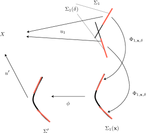
Figure 6. $((\Sigma^{\prime},\vec{z}^{\,\prime}),u^{\prime})$ is $\epsilon$-close to $((\Sigma_{1},\vec{z}_{1}),u_{1})$

This is the definition we used in [FOOO6, FOOO12]. (We remark that this definition and Definition 4.2 are similar to the definition of stable map topology introduced in [FOn].)

The next lemma is sometimes useful to check Definition 7.8 Condition (3).

Lemma 7.9.

Suppose $\delta>\delta^{\prime}>0$ and $\phi:(\Sigma_{1}({\bf x}),\vec{z}_{1}({\bf x})\cup\vec{w}_{1}({\bf x}))\cong(\Sigma^{\prime},\vec{z}^{\,\prime}\cup\vec{w}^{\,\prime})$ is an isomorphism with ${\bf x}=((\rho_{\rm e})_{{\rm e}\in\Gamma(\Sigma)}),(x_{a})_{a\in\mathcal{A}_{s}})\in(\mathcal{V}_{1,0}(\delta^{\prime}/2))\times\mathcal{V}_{1,1}$.

We assume Conditions (1)(2)(3) are satisfied for $\delta$ and $\epsilon$ and the map $u^{\prime}\circ\phi$ is holomorphic outside the image of $\Phi_{1,\bf x,\delta}$.

Then Conditions (1)(2)(3) are satisfied for $\delta^{\prime}$ and $o(\epsilon)$.

Remark 7.10.

Here and hereafter $o(\epsilon)$ is a positive number depending on $\epsilon$ and such that $\lim_{\epsilon\to 0}o(\epsilon)=0$.

Proof.

The conditions (2)(3) for $\delta^{\prime}$ are obvious. The $C^{2}$ norm of the difference between $u^{\prime}\circ\phi\circ\Phi_{1,\bf x,\delta}$ and $u_{1}|_{\Sigma_{1}(\delta)}$ is smaller than $\epsilon$ by assumption. By (1)(3) for $\delta$, the map $u_{1}$ has diameter $<o(\epsilon)$ on $\partial\Sigma_{1}(\delta)$. Since $u^{\prime}\circ\phi$ is holomorphic on $\Sigma_{1}\setminus\Sigma_{1}(\delta)$ it implies that the map $u_{1}$ has diameter $<o(\epsilon)$ on $\Sigma_{1}\setminus\Sigma_{1}(\delta)$. Therefore by (1)(3) again, $C^{0}$ distance between $u^{\prime}\circ\phi\circ\Phi_{1,{\bf x},\delta^{\prime}/2}$ and $u_{1}|_{\Sigma_{1}(\delta^{\prime}/2)}$ is $o(\epsilon)$. Since $u^{\prime}\circ\phi\circ\Phi_{1,{\bf x},\delta^{\prime}/2}$ and $u_{1}$ are both holomorphic on $\Sigma_{1}(\delta^{\prime}/2)\setminus\Sigma_{1}(\delta)$ we can estimate $C^{2}$ distance between them on $\Sigma_{1}(\delta^{\prime})\setminus\Sigma_{1}(\delta)$ by the $C^{0}$ distance between them on $u^{\prime}\circ\phi\circ\Phi_{1,{\bf x},\delta^{\prime}/2}$ and $u_{1}|_{\Sigma_{1}(\delta^{\prime}/2)}$. ∎

Definition 7.11.

Let $((\Sigma_{1},\vec{z}_{1}),u_{1})\in U(((\Sigma,\vec{z}),u);\epsilon_{2})$. Suppose we are given its stabilization and trivialization data ${\mathfrak{W}}$.

We denote by $\mathcal{U}(\epsilon;(\Sigma_{1},\vec{z}_{1}),u_{1},{\mathfrak{W}})$ the set of the isomorphism classes of elements of $U(((\Sigma,\vec{z}),u);\epsilon_{2})$ which is $\epsilon$-close to $((\Sigma_{1},\vec{z}_{1}),u_{1})$ with respect to ${\mathfrak{W}}$.

We will show that the set $\mathcal{U}(\epsilon;(\Sigma_{1},\vec{z}_{1}),u_{1},{\mathfrak{W}})$ has a structure of a smooth orbifold. (We actually show that this is a quotient of a smooth manifold by the action of the group $\mathcal{G}_{1}$.)

The proof is by gluing analysis. To carry out gluing analysis, we study how the obstruction bundle $E((\Sigma^{\prime},\vec{z}^{\,\prime}),u^{\prime})$ behaves when we move $((\Sigma^{\prime},\vec{z}^{\,\prime}),u^{\prime})$. We first take an appropriate parametrization of the set of the triples $((\Sigma^{\prime},\vec{z}^{\,\prime}),u^{\prime})$ which is $\epsilon$-close to $((\Sigma_{1},\vec{z}_{1}),u_{1})$.

We first observe the following.

Lemma 7.12.

The vector space $E((\Sigma^{\prime},\vec{z}^{\,\prime}),u^{\prime})$ depends only on $(\Sigma^{\prime},\vec{z}^{\,\prime})$ and the restriction of $u^{\prime}$ to the image of $\phi\circ\Phi_{1,\bf x,\delta}:\Sigma_{1}(\delta)\to\Sigma_{1}({\bf x})\to\Sigma^{\prime}$, if $\delta$ is small.

Proof.

We remark that the support of elements of $E((\Sigma^{\prime},\vec{z}^{\,\prime}),u^{\prime})$ is in the image of $\phi\circ\Phi_{1,\bf x,\delta}$ by construction.

Moreover for $(\varphi,g)\in\mathcal{W}(\epsilon_{1};{\bf x}_{0},\phi_{0};((\Sigma^{\prime},\vec{z}^{\,\prime}),u^{\prime}))$ the value ${\rm meandist}(\varphi,g)$ of the function ${\rm meandist}$ does not change when we change $u^{\prime}$ outside the image of $\phi\circ\Phi_{1,\bf x,\delta}$. This is an immediate consequence of its definition (6.1).

The lemma follows from these two facts. ∎

Suppose $((\Sigma_{1},\vec{z}_{1}),u_{1})$ is $G$-$\epsilon_{2}$-close to $((\Sigma,\vec{z}),u)$ by $g_{1}$, ${\bf x}_{1}$, $\phi_{1}$. For simplicity of notation we identify $\Sigma({\bf x}_{1})$ with $\Sigma_{1}$ by $\phi_{1}$ and regard $\Sigma_{1}=\Sigma({\bf x}_{1})$.

Let ${\bf x}=(\vec{x},\vec{\rho})\in\mathcal{V}_{(1)}=\mathcal{V}_{1,0}\times\mathcal{V}_{1,1}(\delta)$ where $(x_{a})_{a\in\mathcal{A}_{s}}\in\mathcal{V}_{1,0}$ and $\vec{\rho}=(\rho_{\rm e})_{{\rm e}\in\Gamma(\Sigma_{1})}\in\mathcal{V}_{1,1}(\delta)$.

We consider $(\Sigma_{1}({\bf x}),\vec{z}_{1}({\bf x})\cup\vec{w}_{1}({\bf x}))$.

Hereafter we denote by $\Sigma_{1}({\bf x})(\delta)$ the image of the map $\phi\circ\Phi_{1,\bf x,\delta}:\Sigma_{1}(\delta)\to\Sigma_{1}({\bf x})\to\Sigma^{\prime}$. Let $\hat{u}^{\prime}:\Sigma_{1}(\delta)\to X$ be an $L^{2}_{m+1}$ map which is close to $u_{1}$ in $L^{2}_{m+1}$ norm. We consider

(7.9) $$u^{\prime}=\hat{u}^{\prime}\circ\Phi_{1,{\bf x},\delta}^{-1}:\Sigma_{1}({\bf x})(\delta)\to X.$$

By Lemma 7.12 the subspace

$$E((\Sigma_{1}({\bf x}),\vec{z}_{1}({\bf x})),u^{\prime})\subset L^{2}_{m+1}(\Sigma_{1}({\bf x})(\delta);(u^{\prime})^{*}TX\otimes\Lambda^{01})$$

is well-defined. (Here we use the fact that $u^{\prime}\circ\Phi_{1,{\bf x},\delta}$ is $C^{2}$ close to $u_{1}$. Note $m$ in $L^{2}_{m+1}$ is chosen sufficiently large. So $L^{2}_{m+1}\subset C^{2}$ in particular.)

By assumption

$$d_{X}(u^{\prime}(\Phi_{1,{\bf x},\delta}(z)),u_{1}(z))$$

is small. Therefore we can use parallel transportation (with respect to a $G$-invariant hermitian connection of $TX$) along the minimal geodesic joining $u^{\prime}(\Phi_{1,{\bf x},\delta}(z)))$ to $u_{1}(z)$ to obtain

(7.10) $${\rm Pal}:L^{2}_{m+1}(\Sigma_{1}({\bf x})(\delta);(u^{\prime})^{*}TX)\to L^{2}_{m+1}(\Sigma_{1}(\delta);u_{1}^{*}TX).$$

Moreover using the diffeomorphism $\Phi_{1,{\bf x},\delta}$ we obtain a map

(7.11) $$d^{h}\Phi_{1,{\bf x},\delta}:\Lambda_{\Phi_{1,{\bf x},\delta}(z)}^{01}\Sigma_{1}({\bf x})\to\Lambda_{z}^{01}\Sigma_{1}.$$

in the same way as (6.10).

Using (7.10) and (7.11) we obtain:

(7.12) $$I_{\hat{u}^{\prime},{\bf x}}:L^{2}_{m+1}(\Sigma_{1}({\bf x})(\delta);(u^{\prime})^{*}TX\otimes\Lambda^{01})\to L^{2}_{m+1}(\Sigma_{1}(\delta);u_{1}^{*}TX\otimes\Lambda^{01}).$$

Definition 7.13.

We define

$$E(\hat{u}^{\prime},{\bf x})=I_{\hat{u}^{\prime},{\bf x}}(E((\Sigma_{1}({\bf x}),\vec{z}_{1}({\bf x})),u^{\prime}))\subset L^{2}_{m+1}(\Sigma_{1}(\delta);u_{1}^{*}TX\otimes\Lambda^{01}).$$

Note $E(\hat{u}^{\prime},{\bf x})$ is a finite dimensional subspace of the Hilbert space $L^{2}_{m+1}(\Sigma_{1}(\delta);u_{1}^{*}TX\otimes\Lambda^{01})$, which is independent of $(\hat{u}^{\prime},{\bf x})$. So we can discuss $(\hat{u}^{\prime},{\bf x})$ dependence of $E(\hat{u}^{\prime},{\bf x})$.

Now the main new point we need to check to work out the gluing analysis is the following. We put

$$d=\dim E((\Sigma^{\prime},\vec{z}^{\,\prime}),u^{\prime}).$$

Proposition 7.14.

Let $U^{\prime}(\epsilon)$ be an $\epsilon$ neighborhood of $u_{1}$ in $L^{2}_{m+1}$ norm and $\mathcal{V}_{(1)}(\epsilon)$ an $\epsilon$ neighborhood of $0$ in $\mathcal{V}_{(1)}$.

There exists $d$ smooth maps $e_{i}(\hat{u}^{\prime},{\bf x})$ from $U^{\prime}(\epsilon)\times\mathcal{V}_{(1)}(\epsilon)$ to $L^{2}_{m+1}(\Sigma_{1}(\delta);u_{1}^{*}TX\otimes\Lambda^{01})$ such that for each $\hat{u}^{\prime},{\bf x}$

$$(e_{1}(\hat{u}^{\prime},{\bf x}),\dots,e_{d}(\hat{u}^{\prime},{\bf x}))$$

is a basis of $E(\hat{u}^{\prime},{\bf x})$.

Moreover the $C^{n}$ norm of the map $e_{i}$ is uniformly bounded on $U^{\prime}(\epsilon)\times\mathcal{V}_{(1)}(\epsilon)$ for any $n$.

See Figure 9 in Subsection 7.4.

We prove Proposition 7.14 in Subsection 7.4.

To clarify the fact that Proposition 7.14 gives the control of the behavior of $E(\hat{u}^{\prime},{\bf x})$ needed for the gluing analysis detailed in [FOOO8] to work, we change variables and restate Proposition 7.14 below. We took ${\bf x}=(\vec{x},\vec{\rho})\in\mathcal{V}_{(1)}=\mathcal{V}_{1,0}\times\mathcal{V}_{1,1}$ where $\vec{x}=(x_{a})_{a\in\mathcal{A}_{s}}\in\mathcal{V}_{1,0}$ and $\vec{\rho}=(\rho_{\rm e})_{{\rm e}\in\Gamma(\Sigma_{1})}\in\mathcal{V}_{1,1}(\delta)$. We define $T_{\rm e}$ and $\theta_{\rm e}$ for each ${\rm e}\in\Gamma(\Sigma_{1})$ by the following formula:

(7.13) $$\exp(-10\pi T_{\rm e}) =|\rho_{\rm e}|$$

$$\exp(2\pi\theta_{\rm e}\sqrt{-1}) =\rho_{\rm e}/|\rho_{\rm e}|.$$

Compare [FOOO8, (8.18)]. We thus identify

$$\mathcal{V}_{0,1}(\delta)\cong\prod_{{\rm e}\in\Gamma(\Sigma_{1})}(-\log\delta/10\pi,\infty]\times{\mathbb{R}}/{\mathbb{Z}},$$

using $T_{\rm e}$, $\theta_{\rm e}$ as coordinates. Now we rewrite the smoothness of the map $e_{i}(\hat{u}^{\prime},{\bf x})$ as follows.

Corollary 7.15.

We have an inequality

(7.14) $$\left\|\frac{\partial}{\partial T_{{\rm e}_{1}}}\dots\frac{\partial}{\partial T_{{\rm e}_{n_{1}}}}\frac{\partial}{\partial\theta_{{\rm e}^{\prime}_{1}}}\dots\frac{\partial}{\partial\theta_{{\rm e}^{\prime}_{n_{2}}}}e_{i}\right\|_{C^{n}}$$

$$\leq C_{n,n_{1},n_{2}}\exp\left(-\delta_{n,n_{1},n_{2}}\left(\sum_{i=1}^{n_{1}}T_{{\rm e}_{i}}+\sum_{i=1}^{n_{2}}T_{{\rm e}^{\prime}_{i}}\right)\right).$$

Here $C^{n}$ in the left hand side is the $C^{n}$ norm as a map from $U^{\prime}(\epsilon)\times\mathcal{V}_{1,1}$ to $L^{2}_{m+1}(\Sigma_{1}(\delta);u_{1}^{*}TX\otimes\Lambda^{01})$. In other words, we fix $\vec{\rho}$ (or $T_{\rm e},\theta_{\rm e}$) and regard $\hat{u}^{\prime}$ and $\vec{x}$ as variables to define $C^{n}$ norm.

It is easy to see that the exponential factor in the right hand side appears by the change of variables from $\rho_{\rm e}$ to $(T_{\rm e},\theta_{\rm e})$. So Corollary 7.15 is an immediate consequence of Proposition 7.14.

Corollary 7.15 corresponds to [FOOO8, Proposition 8.19]. This is all the properties we need for the proof of [FOOO8] to work in the case obstruction bundle is given as $E(\hat{u}^{\prime},{\bf x})$. Thus by [FOOO8] we obtain the next two Propositions 7.16 and 7.17. We need to introduce some notations to state them.

We define a linear differential operator

(7.15) $$D_{u_{1}}\overline{\partial}:W^{2}_{m+1}(\Sigma_{1};u_{1}^{*}TX)\to L^{2}_{m}(\Sigma_{1};u_{1}^{*}TX\otimes\Lambda^{01}),$$

in the same way as (4.14).

Condition 4.6 (1) implies that we can choose $\epsilon_{2}$ small such that

$${\rm Im}(D_{u_{1}}\overline{\partial})+E((\Sigma_{1},\vec{z}_{1}),u_{1})=L^{2}_{m}(\Sigma_{1};u_{1}^{*}TX\otimes\Lambda^{01}),$$

if $((\Sigma_{1},\vec{z}_{1}),u_{1})$ is $\epsilon_{2}$-close to $((\Sigma,\vec{z}),u)$.

In the same way as we did in Condition 4.6 (2), we put

(7.16) $${\rm Ker}^{+}D_{u_{1}}\overline{\partial}=\{v\in W^{2}_{m+1}(\Sigma;u_{1}^{*}TX)\mid D_{u_{1}}\overline{\partial}(v)\in E((\Sigma_{1},\vec{z}_{1}),u_{1}).\}$$

This is a finite dimensional space consisting of smooth sections. This space is $\mathcal{G}_{1}$ invariant.

Let $\mathcal{V}_{\rm map}(\epsilon)$ be the $\epsilon$ neighborhood of $0$ in ${\rm Ker}^{+}D_{u_{1}}\overline{\partial}$ and $\mathcal{V}_{(1)}(\epsilon)$ the $\epsilon$ neighborhood of $o$ in $\mathcal{V}_{(1)}$.

Proposition 7.16.

For sufficiently small $\epsilon$ there exists a family of maps

$$u_{{\bf v},{\bf x}}:\Sigma_{1}({\bf x})\to X$$

parametrized by

$$({\bf v},{\bf x})\in\mathcal{V}_{\rm map}(\epsilon)\times\mathcal{V}_{(1)}(\epsilon)$$

with the following properties.

1. The equation

   $$\overline{\partial}u_{{\bf v},{\bf x}}\in E((\Sigma_{1}({\bf x}),\vec{z}_{1}({\bf x})),u_{{\bf v},{\bf x}})$$

   is satisfied. Moreover for each connected component of $\Sigma_{1}({\bf x})\setminus{\rm Im}(\Phi_{1,\bf x,\delta})$ the diameter of its image by $u_{{\bf v},{\bf x}}$ is smaller than $\epsilon$.

2. There exists $\epsilon^{\prime}>0$ such that if $((\Sigma^{\prime},\vec{z}^{\,\prime}\cup\vec{w}^{\,\prime}),u^{\prime})$ satisfies the next four conditions (a)(b)(c)(d) then then there exists ${\bf v}\in\mathcal{V}_{\rm map}(\epsilon)$ such that

   $$u^{\prime}\circ\phi=u_{{\bf v},{\bf x}}.$$

   1. $\overline{\partial}u^{\prime}\in E((\Sigma^{\prime},\vec{z}^{\,\prime}),u^{\prime})$:

   2. $[\Sigma^{\prime},\vec{z}^{\,\prime}\cup\vec{w}^{\,\prime}]\in\mathcal{V}_{(1)}(\epsilon)$:

   3. Let $(\Sigma^{\prime},\vec{z}^{\,\prime}\cup\vec{w}^{\,\prime})\cong(\Sigma_{1}({\bf x}),\vec{z}_{1}({\bf x})\cup\vec{w}_{1}({\bf x}))$ and $\phi$ is the isomorphism. We assume that the $C^{2}$ norm between $u^{\prime}\circ\phi\circ\Phi_{1,\bf x,\delta}$ and $u_{1}|_{\Sigma_{1}(\delta)}$ is smaller than $\epsilon^{\prime}$:

   4. The map $u^{\prime}$ has diameter $<\epsilon$ on $\Sigma^{\prime}\setminus{\rm Im}(\phi\circ\Phi_{1,\bf x,\delta})$.

3. If ${\bf v}\neq{\bf v}^{\prime}$ then $u_{{\bf v},{\bf x}}\neq u_{{\bf v}^{\prime},{\bf x}}$ for any ${\bf x}\in\mathcal{V}_{(1)}(\epsilon)$.

4. If ${\bf v}={\bf 0}$ and ${\bf x}=o$ (the point corresponding to $\Sigma_{1}$) then $u_{{\bf 0},o}=u_{1}$.

The map $({\bf v},{\bf x})\mapsto u_{{\bf v},{\bf x}}$ is $\mathcal{G}_{1}$-equivariant.

Proof.

The construction of the family of maps $u_{{\bf v},{\bf x}}$ satisfying Items (1), (4) above is by alternating method we detailed in [FOOO8, Sections 4 and 5]. (We use the estimate Corollary 7.15 for the proof in [FOOO8].)

(2)(3) are surjectivity and injectivity of the gluing map, respectively, which are proved in [FOOO8, Section 7]. ∎

To state the next proposition we need a notation. We consider the family of maps $u_{{\bf v},{\bf x}}$ in Proposition 7.16. We consider the smooth open embedding

$$\Phi_{1,{\bf x},\delta}:\Sigma_{1}(\delta)\to\Sigma_{1}({\bf x})$$

defined in (7.8). We denote the composition by

(7.17) $${\rm Res}(u_{{\bf v},{\bf x}})=u_{{\bf v},{\bf x}}\circ\Phi_{1,{\bf x},\delta}:\Sigma_{1}(\delta)\to X.$$

We remark that the domain and the target of the map ${\rm Res}(u_{{\bf v},{\bf x}})$ is independent of ${\bf v},{\bf x}$. So we regard ${\bf v},{\bf x}\mapsto{\rm Res}(u_{{\bf v},{\bf x}})$ as a map:

$$\mathcal{V}_{\rm map}(\epsilon)\times\mathcal{V}_{(1)}(\epsilon)\to L^{2}_{m+1}(\Sigma_{1}(\delta),X).$$

Here $L^{2}_{m+1}(\Sigma_{1}(\delta),X)$ is the Hilbert manifold of the maps of $L^{2}_{m+1}$ classes.

Proposition 7.17.

For each $n$, $m>n+10$ the map

$${\bf v},{\bf x}\mapsto{\rm Res}(u_{{\bf v},{\bf x}})$$

is of $C^{n}$ class as a map

$$\mathcal{V}_{\rm map}(\epsilon)\times\mathcal{V}_{(1)}(\epsilon)\to L^{2}_{m+1-n}(\Sigma_{1}(\delta),X).$$

Moreover for $n_{1}+n_{2}\leq n$, $n^{\prime}\leq n$, we have the next estimate

(7.18) $$\left\|\frac{\partial}{\partial T_{{\rm e}_{1}}}\dots\frac{\partial}{\partial T_{{\rm e}_{n_{1}}}}\frac{\partial}{\partial\theta_{{\rm e}^{\prime}_{1}}}\dots\frac{\partial}{\partial\theta_{{\rm e}^{\prime}_{n_{2}}}}u_{{\bf v},{\bf x}}\right\|_{C^{n^{\prime}}}$$

$$\leq C_{n^{\prime},n_{1},n_{2}}\exp\left(-\delta^{\prime}_{n^{\prime},n_{1},n_{2}}\left(\sum_{i=1}^{n_{1}}T_{{\rm e}_{i}}+\sum_{i=1}^{n_{2}}T_{{\rm e}^{\prime}_{i}}\right)\right).$$

Here the $C^{n^{\prime}}$ norm in the left hand side is defined as follows. We regard the $T$ and $\theta$ differential of $u_{{\bf v},{\bf x}}$ as a map

$$\mathcal{V}_{\rm map}(\epsilon)\times\mathcal{V}_{(1)}(\epsilon)\to L^{2}_{m+1-n}(\Sigma_{1}(\delta),X).$$

Then $\|\|_{C^{n^{\prime}}}$ is the $C^{n^{\prime}}$ norm the map in the left hand side for a fixed $T_{\rm e}$ and $\theta_{\rm e}$.

Proof.

This is [FOOO8, Theorem 6.4]. ∎

Remark 7.18.

We remark that the number $\delta^{\prime}_{n^{\prime},n_{1},n_{2}}$ appearing in Proposition 7.17 is different from $\delta_{n^{\prime},n_{1},n_{2}}$ in (7.14). Actually (7.18) does not imply the smooth-ness of $u_{{\bf v},{\bf x}}$ with respect to $\rho_{\rm e}$ in (7.13). See [FOOO2, Remark A1.63]. This is the reason why we will change the smooth structure in Definition 7.19.

7.2. Construction of the smooth chart 2: Construction of smooth chart at one point of $U(((\Sigma,\vec{z}),u);\epsilon_{2})$

We now use Propositions 7.16 and 7.17 to construct a smooth structure at each point of $U(((\Sigma,\vec{z}),u);\epsilon_{2})$. Let $((\Sigma_{1},\vec{z}_{1}),u_{1})\in U(((\Sigma,\vec{z}),u);\epsilon_{2})$. Let ${\mathfrak{W}}$ be its stabilization and trivialization data.

We obtain a map

$${\bf v},{\bf x}\mapsto{\rm Res}(u_{{\bf v},{\bf x}})\,\,:\,\mathcal{V}_{\rm map}(\epsilon)\times\mathcal{V}_{(1)}(\epsilon)\to L^{2}_{m+1}(\Sigma_{1}(\delta),X).$$

We define a smooth structure on $\mathcal{V}_{(1)}(\epsilon)$ as follows. Note $(T_{\rm e},\theta_{\rm e})_{{\rm e}\in\Gamma(\Sigma_{1})}$ is the coordinate of $\mathcal{V}_{(1)}(\epsilon)$, where $T_{\rm e}\in(\log\delta/10,\infty]\times{\mathbb{R}}/{\mathbb{Z}}$. We put

(7.19) $$\mathfrak{s}_{\rm e}=\frac{e^{2\pi\theta_{\rm e}\sqrt{-1}}}{T_{\rm e}}\in{\mathbb{C}}.$$

Definition 7.19.

We define a $C^{\infty}$ structure on $\mathcal{V}_{1,1}$ such that $(\mathfrak{s}_{\rm e})_{{\rm e}\in\Gamma(\Sigma_{1})}$ is a smooth coordiante.

We put a standard $C^{\infty}$ structure on $\mathcal{V}_{\rm map}(\epsilon)$ and $\mathcal{V}_{1,0}$. Note $\mathcal{V}_{\rm map}(\epsilon)$ is an open subset of a finite dimensional vector space and $\mathcal{V}_{1,0}$ is a product of open neighborhoods of smooth points of the moduli spaces of marked curves (without node). So they have canonical smooth structure. Thus the smooth structure of $\mathcal{V}_{(1)}$ and of its open subset $\mathcal{V}_{(1)}(\epsilon)$ is defined.

Definition 7.20.

We define the evaluation map

$$({\rm EV}_{w_{1,j}})_{j=1,\dots,k}:\mathcal{V}_{\rm map}(\epsilon)\times\mathcal{V}_{(1)}(\epsilon)\to X^{k}.$$

by

$${\rm EV}_{w_{1,j}}({\bf v},{\bf x})=u_{{\bf v},{\bf x}}(w_{1,j}({\bf x})).$$

(We remark that $(w_{1,j}({\bf x})=\mathfrak{t}_{\ell+j}({\bf x})\in\Sigma_{1}({\bf x})$.)

Lemma 7.21.

If $\epsilon$ is sufficiently small then $({\rm EV}_{w_{1,j}})_{j=1,\dots,k}$ is transversal to $\prod_{j}\mathcal{N}_{j}$.

Proof.

Proposition 7.17 implies that the map $({\rm EV}_{w_{1,j}})_{j=1,\dots,k}$ is of $C^{n}$ class for any fixed $n$ with respect to the smooth structure in Definition 7.19, if $\epsilon$ is sufficiently small. (We work using $L^{2}_{m+1}$ spaces with $m$ sufficiently large compared to $n$.) In fact

$${\rm EV}_{w_{1,j}}({\bf v},{\bf x})={\rm Res}(u_{{\bf v},{\bf x}})(\Phi^{-1}_{1,{\bf x},\delta}(w_{1,j}({\bf x})))$$

and ${\bf x}\mapsto\Phi^{-1}_{1,{\bf x},\delta}(w_{1,j}({\bf x}))$ is a smooth map $:\mathcal{V}_{(1)}(\epsilon)\to\Sigma_{1}(\delta)$.

Therefore it suffices to show the lemma at origin (which corresponds to $((\Sigma_{1},\vec{z}_{1}\cup\vec{w}_{1}),u_{1})$). We consider the submanifold $Y$ of $\mathcal{V}_{(1)}(\epsilon)$ which consists of elements $(\Sigma_{1},\vec{z}_{1}\cup\vec{w}^{\,\prime}_{1})$ where $(\Sigma_{1},\vec{z}_{1})$ is the nodal curve with marked points which we take at the beginning of this section, and $w^{\prime}_{1,j}$ is in a neighborhood of $w_{1,j}$. This is a $2k$ dimensional submanifold. (Here $2k$ is the number of parameters to move $k$ points $w^{\prime}_{1,j}$ on Riemann surface.) The restriction of $({\rm EV}_{w_{1,j}})_{j=1,\dots,k}$ to $\{{\bf 0}\}\times\{{\bf 0}\}\times Y$ can be identified with the map

(7.20) $$\vec{w}^{\,\prime}_{1}\mapsto(u_{1}(w^{\prime}_{1,j}))_{j=1,\dots,k}.$$

Note $E(\Sigma_{1}({\bf x}),\vec{z}_{1}({\bf x}))$ is independent of $w^{\prime}_{1,j}$. Therefore, by construction, (that is, the proof of Proposition 7.16 by Newton’s iteration) for all $w^{\prime}_{1,j}$

$$u_{{\bf 0},[\Sigma_{1},\vec{z}_{1}\cup w^{\prime}_{1,j}]}=u_{1}.$$

(Here we regard $[\Sigma_{1},\vec{z}_{1}\cup w^{\prime}_{1,j}]$ as an element of $\{{\bf 0}\}\times Y$.)

By Definition 7.1 (6) the map (7.20) is transversal to $\prod_{j}\mathcal{N}_{j}$. ∎

Definition 7.22.

Let $({\mathfrak{W}},\vec{\mathcal{N}})$ be strong stabilization data at $((\Sigma_{1},\vec{z}_{1}),u_{1})$. We put

$$V(((\Sigma_{1},\vec{z}_{1}),u_{1});\epsilon,({\mathfrak{W}},\vec{\mathcal{N}}))$$

$$=\{({\bf v},{\bf x})\in\mathcal{V}_{\rm map}(\epsilon)\times\mathcal{V}_{(1)}(\epsilon)\mid{\rm EV}_{w_{1,j}}({\bf v},{\bf x})\in\mathcal{N}_{j},\,\,\,j=1,\dots,k\}.$$

We take $\epsilon$ sufficiently small so that conclusion of Lemma 7.21 holds.

Lemma 7.23.

For each sufficiently small $\epsilon_{3}$ there exists $\epsilon$ with the following properties. If

$$[(\Sigma^{\prime},\vec{z}^{\,\prime}),u^{\prime}]\in\mathcal{U}(\epsilon;(\Sigma_{1},\vec{z}_{1}),u_{1},{\mathfrak{W}})$$

then there exists an additional marked points $\vec{w}^{\,\prime}$ and an element $({\bf v},{\bf x})$ of the space $V(((\Sigma_{1},\vec{z}_{1}),u_{1});\epsilon_{3},({\mathfrak{W}},\vec{\mathcal{N}}))$ such that

$$((\Sigma_{1}({\bf x}),\vec{z}_{1}({\bf x})\cup\vec{w}_{1}({\bf x})),u_{{\bf v},{\bf x}})\cong((\Sigma^{\prime},\vec{z}^{\,\prime}\cup\vec{w}^{\,\prime}),u^{\prime}).$$

Namely there exists a bi-holomorphic map $\phi:(\Sigma_{1}({\bf x}),\vec{z}_{1}({\bf x})\cup\vec{w}_{1}({\bf x}))\cong(\Sigma^{\prime},\vec{z}^{\,\prime}\cup\vec{w}^{\,\prime})$ with $u^{\prime}\circ\phi=u_{{\bf v},{\bf x}}$.

Moreover such $({\bf v},{\bf x})\in V(((\Sigma_{1},\vec{z}_{1}),u_{1});\epsilon_{3},({\mathfrak{W}},\vec{\mathcal{N}}))$ is unique up to $\mathcal{G}_{1}$ action.

Proof.

We first prove the existence. Let $\vec{w}^{\,\prime\prime}$ and $\phi^{\prime}:(\Sigma_{1}({\bf x}^{\prime}),\vec{z}_{1}({\bf x}^{\prime})\cup\vec{w}_{1}({\bf x}^{\prime}))\cong(\Sigma^{\prime},\vec{z}^{\,\prime}\cup\vec{w}^{\,\prime\prime})$ be the isomorphism as in Definition 7.8. (We write ${\bf x}^{\prime}$ and $\vec{w}^{\,\prime\prime}$ here instead of ${\bf x}$ and $\vec{w}^{\,\prime}$ in Definition 7.8.)

Note $u^{\prime}(w^{\,\prime\prime}_{j})$ is close to $u_{1}(w_{1,j})$ and $u_{1}(w_{1,j})\in\mathcal{N}_{j}$. Moreover $u^{\prime}$ is $C^{1}$ close to $u_{1}|_{\Sigma_{1}(\delta)}$. Therefore by Definition 7.1 (6) we can find $w^{\,\prime}_{j}$ which is close to $w^{\,\prime\prime}_{j}$ such that $u^{\prime}(w^{\,\prime}_{j})\in\mathcal{N}_{j}$.

Then there exists ${\bf x}$ which is close to ${\bf x}^{\prime}$ and a bi-holomorphic map $\phi:(\Sigma_{1}({\bf x}),\vec{z}_{1}({\bf x})\cup\vec{w}_{1}({\bf x}))\cong(\Sigma^{\prime},\vec{z}^{\,\prime}\cup\vec{w}^{\,\prime})$.

Using Proposition 7.16 (2), there exists ${\bf v}$ such that

$$u^{\prime}\circ\phi=u_{{\bf v},{\bf x}}.$$

Since $u^{\prime}(w^{\,\prime}_{j})\in\mathcal{N}_{j}$ we have

$$u_{{\bf v},{\bf x}}(w^{\,\prime}_{j}({\bf x}))\in\mathcal{N}_{j}.$$

Therefore $({\bf v},{\bf x})\in V(((\Sigma_{1},\vec{z}_{1}),u_{1});({\mathfrak{W}},\vec{\mathcal{N}}))$ as required.

We next prove the uniqueness. Let $({\bf v}^{(i)},{\bf x}^{(i)})\in V(((\Sigma_{1},\vec{z}_{1}),u_{1});\epsilon_{3},({\mathfrak{W}},\vec{\mathcal{N}}))$ ($i=1,2$) and $\vec{w}^{\,\prime}_{(i)}$ ($i=1,2$) both have the required properties.

We observe

$$(\Sigma_{1}({\bf x}^{(1)}),\vec{z}_{1}({\bf x}^{(1)}))\overset{\phi^{(1)}}{\cong}(\Sigma^{\prime},\vec{z}^{\,\prime})\overset{(\phi^{(2)})^{-1}}{\cong}(\Sigma_{1}({\bf x}^{(2)}),\vec{z}_{1}({\bf x}^{(2)}))$$

and

(7.21) $$u^{\prime}\circ\phi^{(i)}=u_{{\bf v}^{(i)},{\bf x}^{(i)}}.$$

Moreover the $C^{2}$ distance between $u^{\prime}\circ\phi^{(i)}\circ\Phi_{1,{\bf x}^{(i)},\delta}$ and $u_{1}$ on $\Sigma_{1}(\delta)$ is smaller than $o(\epsilon_{3})$.

By taking $\epsilon_{3}$, $\delta^{\prime}$ small the composition $\phi=\Phi_{1,{\bf x}^{(2)},\delta^{\prime}}^{-1}\circ(\phi^{(2)})^{-1}\circ\phi^{(1)}\circ\Phi_{1,{\bf x}^{(1)},\delta}$ is defined on $\Sigma_{1}(\delta)$. Then the $C^{2}$ distance between $u_{1}\circ\phi$ and $u_{1}$ as maps on $\Sigma_{1}(\delta)$ is smaller than $o(\epsilon_{3})$. (Note using Lemma 7.9 the $C^{2}$ distance between $u^{\prime}\circ\phi^{(i)}\circ\Phi_{1,{\bf x}^{(i)},\delta}$ and $u_{1}$ on $\Sigma_{1}(\delta^{\prime})$ is still smaller than $o(\epsilon_{3})$. We use this fact.)

Sublemma 7.24.

If $\epsilon$ and $\delta$ are sufficiently small then there exists $v\in\mathcal{G}_{1}$ such that the $C^{2}$ distance between $\phi$ and $v$ is smaller than $o(\epsilon_{3})+o(\delta)$.

Proof.

Suppose the sublemma is false. Then there exist ${\bf x}_{c}^{(i)}$, ${\bf v}_{c}^{(i)}$ (for $i=1,2$) and $u^{\prime}_{c}:\Sigma^{\prime}_{c}\to X$ such that:

1. $\lim_{c\to\infty}{\bf x}_{c}^{(i)}=o=[\Sigma_{1},\vec{z}_{1}]$, $\lim_{c\to\infty}{\bf v}_{c}^{(i)}={\bf 0}$.

2. $u^{\prime}_{c}\circ\phi_{c}^{(i)}=u_{{\bf v}_{c}^{(i)},{\bf x}_{c}^{(i)}}$.

3. We consider $\phi_{c}^{(i)}:(\Sigma_{1}({\bf x}_{c}^{(i)}),\vec{z}_{1}({\bf x}_{c}^{(i)}))\cong(\Sigma^{\prime}_{c},\vec{z}_{c}^{\,\prime})$ and the composition

   $$\phi_{c}=(\phi_{c}^{(1)})^{-1}\circ\phi_{c}^{(2)}.$$

   Then the limit $\lim_{c\to\infty}\phi_{c}$ is not an element of $\mathcal{G}_{1}$ even after taking a subsequence.

We regard $\phi_{c}$ as a map

$$\phi_{c}:\Sigma_{1}({\bf x}^{(2)}_{c})\to\mathcal{C}_{(1)}$$

where $\mathcal{C}_{(1)}$ is the total space of the universal deformation of $(\Sigma_{1},\vec{z}_{1})$. The energy of this map $\phi_{c}$ is uniformly bounded. Therefore we can use Gromov’s compactness theorem [FOn, Theorem 11.1] to find its limit (with respect to the stable map topology), which is a stable map

$$\phi_{\infty}:(\widehat{\Sigma}_{1},\widehat{\vec{z}}_{1})\to(\Sigma_{1},\vec{z}_{1})$$

such that $\widehat{\Sigma}_{1}$ is ${\Sigma}_{1}$ plus bubbles, namely $\widehat{\Sigma}_{1}\to{\Sigma}_{1}$ exists. Suppose $\widehat{\Sigma}_{1}\neq{\Sigma}_{1}$. Then there exists a sphere component $S^{2}_{a}$ of $\widehat{\Sigma}_{1}$ which is unstable. The map $\phi_{\infty}$ is non-constant on $S^{2}_{a}$. Let $S^{2,\prime}_{a}=\phi_{\infty}(S^{2}_{a})\subset{\Sigma}_{1}$ be the image. Since $S^{2,\prime}_{a}$ is unstable the map $u_{{\bf v}^{(2)},{\bf x}_{c}^{(2)}}$ is non-constant there. Therefore the diameter of the image of $u^{\prime}_{c}$ on $\Phi_{1,{\bf x}^{(2)}_{c},\delta}(S^{2}_{a})$ is uniformly away from $0$. Since $S^{2}_{a}$ shrink to a point in $\Sigma_{1}$ the image of $\Phi_{1,{\bf x}^{(2)}_{c},\delta}(S^{2}_{a})$ has diameter $\to 0$ as $c\to\infty$. This is impossible since

(7.22) $$\lim_{c\to\infty}u^{\prime}_{c}\circ\phi^{(i)}_{c}\circ\Phi_{1,{\bf x}_{c}^{(i)},\delta}=u_{1}.$$

on $\Sigma_{1}(\delta)$.

Therefore $\widehat{\Sigma}_{1}=\Sigma_{1}$ and $\phi_{\infty}:{\Sigma}_{1}\to\Sigma_{1}$ is an isomorphism. We use (7.22) to obtain $u_{1}\circ\phi_{\infty}=u_{1}$. Namely $\phi_{\infty}\in\mathcal{G}_{1}$. This is a contradiction. ∎

Using $\mathcal{G}_{1}$ equivariance of the map $({\bf v},{\bf x})\mapsto u_{{\bf v},{\bf x}}$ in Proposition 7.16 we may assume that $v=1$, by replacing ${\bf x}^{(2)}$ etc. if necessary. In other words, we may assume $\phi^{(2)}\circ\Phi_{1,{\bf x}^{(2)},\delta}$ is $C^{2}$ close to $\phi^{(1)}\circ\Phi_{1,{\bf x}^{(2)},\delta}$.

By assumption

$$\vec{w}^{\,\prime}_{(i)}=\phi^{(i)}(w_{1,j}({\bf x}^{(i)})).$$

On the other hand

(7.23) $$d(w_{1,j}({\bf x}^{(i)}),\Phi_{1,{\bf x}^{(i)},\delta}(w_{1,j}))<o(\epsilon_{3}).$$

Here $d$ is a metric on $\Sigma({\bf x}^{(i)})$ which is the restriction of a metric of the total space of the universal family of deformation of $(\Sigma_{i},\vec{z}_{i}\cup\vec{w}_{i})$.

(7.23) follows from the fact that $\Phi_{1,{\bf x}^{(i)},\delta}$ converges to the identity map as ${\bf x}^{(i)}$ converges to ${\bf o}_{i}=[\Sigma_{i},\vec{z}_{i}\cup\vec{w}_{i}]$ and $w_{1,j}({\bf x}^{(i)})$ converges to $w_{i,j}$ as ${\bf x}^{(i)}$ converges to $o_{i}$.

Remark 7.25.

Note $w_{1,j}({\bf x}^{(i)})\neq\Phi_{1,{\bf x}^{(i)},\delta}(w_{1,j})$ in general since we do not assume Definition 7.2 (4) for marked points of $(\Sigma_{1})_{a}$ other than nodal points of $\Sigma_{1}$.

Therefore $\vec{w}^{\,\prime}_{(1)}$ is close to $\vec{w}^{\,\prime}_{(2)}$ in $\Sigma^{\prime}$. Furthermore we have

$$u^{\prime}(\vec{w}^{\,\prime}_{(1)}),u^{\prime}(\vec{w}^{\,\prime}_{(2)})\in\mathcal{N}_{j}.$$

Using also Definition 7.1 (6) it implies that

$$\vec{w}^{\,\prime}_{(1)}=\vec{w}^{\,\prime}_{(2)}.$$

Therefore

$$(\Sigma_{1}({\bf x}^{(1)}),\vec{z}_{1}({\bf x}^{(1)})\cup\vec{w}_{1}({\bf x}^{(1)})) \overset{\phi^{(1)}}{\cong}(\Sigma^{\prime},\vec{z}^{\,\prime}\cup\vec{w}^{\,\prime}_{(1)})=(\Sigma^{\prime},\vec{z}^{\,\prime}\cup\vec{w}^{\,\prime}_{(2)})$$

$$\overset{(\phi^{(2)})^{-1}}{\cong}(\Sigma_{1}({\bf x}^{(2)}),\vec{z}_{1}({\bf x}^{(2)})\cup\vec{w}_{1}({\bf x}^{(2)})).$$

Thus ${\bf x}^{(1)}={\bf x}^{(2)}$. Now Proposition 7.16 (3) implies ${\bf v}^{(1)}={\bf v}^{(2)}$. The proof of the uniqueness is complete. ∎

Lemma 7.23 implies that the set $\mathcal{U}(\epsilon;(\Sigma_{1},\vec{z}_{1}),u_{1},{\mathfrak{W}})$ is identified with a neighborhood of the origin of the quotient space

(7.24) $$V(((\Sigma_{1},\vec{z}_{1}),u_{1});\epsilon_{3},({\mathfrak{W},\vec{\mathcal{N}})})/\mathcal{G}_{1}.$$

Thus $\mathcal{U}(\epsilon;(\Sigma_{1},\vec{z}_{1}),u_{1},{\mathfrak{W}})$ has an orbifold chart. By Proposition 7.14 there exists a smooth vector bundle (orbibundle) $E(((\Sigma_{1},\vec{z}_{1}),u_{1});\epsilon_{3},{\mathfrak{W}})$ on (7.24) such that the fiber of $((\Sigma^{\prime},\vec{z}^{\,\prime}),u^{\prime})$ is identified with $E((\Sigma^{\prime},\vec{z}^{\,\prime}),u^{\prime})$. Moreover it implies that the map which associate to $((\Sigma^{\prime},\vec{z}^{\,\prime}),u^{\prime})$ the element

$$s((\Sigma^{\prime},\vec{z}^{\,\prime}),u^{\prime})=\overline{\partial}u^{\prime}\in E((\Sigma^{\prime},\vec{z}^{\,\prime}),u^{\prime})$$

is a smooth section of $E((\Sigma^{\prime},\vec{z}^{\,\prime}),u^{\prime})$.

We define

$$\psi((\Sigma^{\prime},\vec{z}^{\,\prime}),u^{\prime})=[(\Sigma^{\prime},\vec{z}^{\,\prime}),u^{\prime}]\in\mathcal{M}_{g,\ell}((X,J);\alpha)$$

if $((\Sigma^{\prime},\vec{z}^{\,\prime}),u^{\prime})$ is an element of (7.24) with $s((\Sigma^{\prime},\vec{z}^{\,\prime}),u^{\prime})=0$. This defines a parametrization map

$$\psi:s^{-1}(0)/\mathcal{G}_{1}\to\mathcal{M}_{g,\ell}((X,J);\alpha).$$

Now we sum up the conclusion of this subsection as follows.

Proposition 7.26.

For each $n$ there exists $\epsilon_{(n)}$ such that

$$(V(((\Sigma_{1},\vec{z}_{1}),u_{1});\epsilon_{(n)},({\mathfrak{W}},\vec{\mathcal{N}}))/\mathcal{G}_{1},E(((\Sigma_{1},\vec{z}_{1}),u_{1});\epsilon_{(n)},({\mathfrak{W}},\vec{\mathcal{N}})),s,\psi)$$

is a Kuranishi neighborhood of $C^{n}$ class at $[((\Sigma_{1},\vec{z}_{1}),u_{1})]$ of $\mathcal{M}_{g,\ell}((X,J);\alpha)$.

In the next subsection we use it to define a $G$-equivariant Kuranishi chart containing the $G$ orbit of $[(\Sigma,\vec{z}),u]$.

7.3. Construction of the smooth chart 3: Proof of Proposition 6.15

We first define a topology of the set $U(((\Sigma,\vec{z}),u);\epsilon_{2})$. We use the sets $\mathcal{U}(\epsilon;(\Sigma_{1},\vec{z}_{1}),u_{1},{\mathfrak{W}})$ defined in Definition 7.11 for this purpose.

Lemma 7.27.

Suppose $((\Sigma_{2},\vec{z}_{2}),u_{2})\in\mathcal{U}(\epsilon;(\Sigma_{1},\vec{z}_{1}),u_{1},{\mathfrak{W}}^{(1)})$.

Then there exists $\epsilon^{\prime}>0$ such that

(7.25) $$\mathcal{U}(\epsilon^{\prime};(\Sigma_{2},\vec{z}_{2}),u_{2},{\mathfrak{W}}^{(2)})\subset\mathcal{U}(\epsilon;(\Sigma_{1},\vec{z}_{1}),u_{1},{\mathfrak{W}}^{(1)}).$$

Proof.

We prove this lemma in Subsection 7.5. ∎

Proposition 7.28.

There exists a topology of $U(((\Sigma,\vec{z}),u);\epsilon_{2})$ such that the family of its subsets,

(7.26) $$\{\mathcal{U}(\epsilon;(\Sigma_{1},\vec{z}_{1}),u_{1},{\mathfrak{W}}^{(1)})\mid\epsilon>0,((\Sigma_{1},\vec{z}_{1}),u_{1}),{\mathfrak{W}}^{(1)}\}$$

is a basis of the topology.

This topology is Hausdorff.

Proof.

The existence of the topology for which (7.26) is a basis of neighborhood system is a consequence of Lemma 7.27. (See for example [Ke, Theorem 11, p47].)

We also remark that Lemma 7.27 implies that for any ${\mathfrak{W}}^{(1)}$, the set $U$ containing $[(\Sigma_{1},\vec{z}_{1}),u_{1}]$ is a neighborhood of $[(\Sigma_{1},\vec{z}_{1}),u_{1}]$ if and only if $\mathcal{U}(\epsilon;(\Sigma_{1},\vec{z}_{1}),u_{1},{\mathfrak{W}}^{(1)})\subset U$ for sufficiently small $\epsilon$.

We next prove that this topology is Hausdorff. Let $[(\Sigma_{i},\vec{z}_{i}),u_{i}]\in U(((\Sigma,\vec{z}),u);\epsilon_{2})$ and ${\mathfrak{W}}^{(i)}$ stabilization and trivialization data, for $i=1,2$. We assume $[(\Sigma_{1},\vec{z}_{1}),u_{1}]\neq[(\Sigma_{2},\vec{z}_{2}),u_{2}]$. It suffices to show that

$$\mathcal{U}(\epsilon;(\Sigma_{1},\vec{z}_{1}),u_{1},{\mathfrak{W}}^{(1)})\cap\mathcal{U}(\epsilon;(\Sigma_{2},\vec{z}_{2}),u_{2},{\mathfrak{W}}^{(2)})=\emptyset$$

for sufficiently small $\epsilon$. Suppose this does not hold.

We consider the universal family of deformation of $(\Sigma,\vec{z})$ produced by Theorem 3.5. Then there exist $o(c)\to 0$, ${\bf x}_{c}\in\mathcal{OB}$ and $u_{c}:\Sigma({\bf x}_{c})\to X$, such that $[(\Sigma({\bf x}_{c}),\vec{z}({\bf x}_{c})),u_{c}]$ lies in

$$\mathcal{U}(\epsilon(c);(\Sigma_{1},\vec{z}_{1}),u_{1},{\mathfrak{W}}^{(1)})\cap\mathcal{U}(\epsilon(c);(\Sigma_{2},\vec{z}_{2}),u_{2},{\mathfrak{W}}^{(2)}).$$

We may take ${\bf x}_{c}\in\mathcal{OB}$ and $u_{c}:\Sigma({\bf x}_{c})\to X$ such that ${\rm meandist}$ attains its minimum at $((\Sigma({\bf x}_{c}),\vec{z}({\bf x}_{c})),u_{c})$.

Remark 7.29.

More precisely ‘${\rm meandist}$ attains its minimum at $((\Sigma({\bf x}_{c}),\vec{z}({\bf x}_{c})),u_{c})$’ means the following. We consider ${\rm id}:(\Sigma({\bf x}_{c}),\vec{z}({\bf x}_{c}))\cong(\Sigma({\bf x}_{c}),\vec{z}({\bf x}_{c}))$ in Definition 6.1. In other words we consider the case $((\Sigma^{\prime},\vec{z}^{\,\prime}),u^{\prime})=((\Sigma({\bf x}_{c}),\vec{z}({\bf x}_{c}),u_{c})$ and ${\bf x}_{0}={\bf x}_{c}$, $\phi_{0}={\rm id}$. We then obtain

$${\rm meandist}:\mathcal{W}(\epsilon_{1};{\bf x}_{c},{\rm id};(\Sigma({\bf x}_{c}),\vec{z}({\bf x}_{c})),u_{c}))\to{\mathbb{R}}$$

by Definition 6.5. We require that at

$$(\varphi,g)=(\mathcal{ID}({\bf x}_{c}),g)\in\mathcal{W}(\epsilon_{1};{\bf x}_{c},{\rm id};(\Sigma({\bf x}_{c}),\vec{z}({\bf x}_{c}),u_{c}))$$

the function ${\rm meandist}$ attains its minimum, for some $g$.

By Definition 7.8, there exists $\vec{w}_{i}(c)\subset\Sigma({\bf x}_{c})$, ${\bf y}_{i,c}\in\mathcal{V}^{(i)}_{1,0}\times\mathcal{V}^{(i)}_{1,1}(\delta_{i}(c))$, (Here we put superscript $(i)$ to indicate that the right hand side is associated with ${\mathfrak{W}}^{(i)}$.) and a bi-holomorphic map

(7.27) $$\phi_{i,c}:(\Sigma_{i}({\bf y}_{i,c}),\vec{z}_{i}({\bf y}_{i,c})\cup\vec{w}_{i}({\bf y}_{i,c}))\cong(\Sigma({\bf x}_{c}),\vec{z}({\bf x}_{c})\cup\vec{w}_{i}(c))$$

with the following properties.

1. The $C^{2}$ norm of the difference between $u_{c}\circ\phi_{i,c}\circ\Phi_{i,{\bf y}_{i,c},\delta_{i}(c)}$ and $u_{i}|_{\Sigma_{i}(\delta_{i}(c))}$ is smaller than $o(c)$. Here

   $$\Phi_{i,{\bf y}_{i,c},\delta_{i}(c)}:\Sigma_{i}(\delta_{i}(c))\to\Sigma_{i}({\bf y}_{i,c})$$

   is obtained from ${\mathfrak{W}}^{(i)}$.

2. The distance between ${\bf y}_{i,c}$ and $[\Sigma_{i},\vec{z}_{i}\cup\vec{w}_{i}]$ in $\mathcal{M}_{g,k_{i}+\ell}$ is smaller than $o(c)$. Moreover $\delta_{i}(c)<o(c)$. (Here $k_{i}=\#\vec{w}_{i}$.)

3. The map $u_{c}\circ\phi_{i,c}$ has diameter $<o(c)$ on $\Sigma_{i}({\bf y}_{i,c})\setminus{\rm Im}(\Phi_{i,{\bf y}_{i,c},\delta_{i}(c)})$.

Remark 7.30.

Here and hereafter, the positive numbers $o(c)$ depend on $c$ and satisfies $\lim_{c\to\infty}o(c)=0$.

Using Lemma 7.9 we may assume $\lim_{c\to\infty}\delta_{i}(c)=0$.

By Definition 7.1 (8), the point $w_{i,j}(c)$ (which is the $j$-th member of $\vec{w}_{i}(c)$) is contained in the image of $\Phi_{{\bf x}_{c},\delta_{i}(c)}:\Sigma(\delta_{i}(c))\to\Sigma({\bf x}_{c})$. We take $\tilde{w}_{i,j}(c)\in\Sigma(\delta_{i}(c))$ such that

$$\Phi_{{\bf x}_{c},\delta_{i}(c)}(\tilde{w}_{i,j}(c))=w_{i,j}(c).$$

By taking a subsequence if necessary we may assume that the limit

(7.28) $$\lim_{c\to\infty}{\bf x}_{c}={\bf x}_{\infty}\in\mathcal{OB}$$

exists. Moreover we may assume

(7.29) $$\lim_{c\to\infty}\Phi_{{\bf x}_{c},\delta_{i}(c)}(\tilde{w}_{i,j}(c))=w_{i,j}(\infty)\in\Sigma({\bf x}_{\infty})$$

converges by taking a subsequence if necessary. Here (7.29) is the convergence in the total space of the universal family of deformation of $(\Sigma,\vec{z})$.

Sublemma 7.31.

$w_{i,j}(\infty)\neq w_{i,j^{\prime}}(\infty)$ if $j\neq j^{\prime}$.

Proof.

We can prove the sublemma by using minimality of ${\rm meandist}$ as follows. Suppose $w_{i,j}(\infty)=w_{i,j^{\prime}}(\infty)$ with $j\neq j^{\prime}$. We may assume $w_{i,j}$ and $w_{i,j^{\prime}}$ are in the same irreducible component of $\Sigma_{i}$, by replacing $j,j^{\prime}$ if necessary. (Here $w_{i,j}$ is the $j$-th member of $\vec{w}_{i}\subset\Sigma_{i}$.) In fact suppose $w_{i,j}$ and $w_{i,j^{\prime}}$ are in the different irreducible components. If there exists $j^{\prime\prime}\neq j$ (resp. $j^{\prime\prime}\neq j^{\prime}$) such that $w_{i,j}$ and $w_{i,j^{\prime\prime}}$ (resp. $w_{i,j^{\prime}}$ and $w_{i,j^{\prime\prime}}$) are in the same irreducible component, then we may replace $w_{i,j^{\prime}}$ by $w_{i,j^{\prime\prime}}$ (resp. $w_{i,j}$ and $w_{i,j^{\prime\prime}}$).

If there exists no such $j^{\prime\prime}$ then one of the following holds because $(\Sigma_{i},\vec{z}_{i}\cup\vec{w}_{i})$ is stable. Let $\Sigma_{ij}$ (resp. $\Sigma_{ij^{\prime}}$) be the irreducible component containing $w_{i,j}$ (resp. $w_{i,j^{\prime}}$).

1. There exist a marked point $z_{i,k_{j}}$ on $\Sigma_{ij}$.

2. The genus of $\Sigma_{ij}$ is positive.

We may assume ${\rm(j^{\prime},I)}$ or ${\rm(j^{\prime},II)}$ also.

If ${\rm(j,I)}$ and ${\rm(j^{\prime},I)}$ hold then since $z_{i,k_{j}}\neq z_{i,k_{j^{\prime}}}$ then $w_{i,j}(\infty)\neq w_{i,j^{\prime}}(\infty)$ and we are done. In the other 3 cases we can show $w_{i,j}(\infty)\neq w_{i,j^{\prime}}(\infty)$ in a similar way.

We thus may assume that $w_{i,j}$ and $w_{i,j^{\prime}}$ are in the same irreducible component of $\Sigma_{i}$.

Moreover the map $u_{i}$ is non-constant on the irreducible component containing $w_{i,j}$ by Definition 7.1 (3). Therefore by Item (1) the map $u_{c}$ has some nontrivial energy in a small neighborhood of $\{w_{i,j}(c),w_{i,j^{\prime}}(c)\}$. (The energy there can be estimated uniformly from below because it is larger than the half of the energy of nontrivial holomorphic sphere for example.)

This implies that the total energy of $u_{c}$ outside a small neighborhood of the set $\{w_{i,j}(c),w_{i,j^{\prime}}(c)\}$ is uniformly strictly smaller than the energy of $u$. Therefore ${\rm meandist}$ is greater than some number independent of $\epsilon_{1}$. If $\epsilon_{1}$ is small then ${\rm meandist}$ does not attain its minimum at $((\Sigma({\bf x}_{c}),\vec{z}({\bf x}_{c})),u_{c})$. This contradicts to our choice. ∎

Sublemma 7.32.

$(\Sigma({\bf x}_{\infty}),\vec{z}({\bf x}_{\infty})\cup\vec{w}_{i}({\infty}))$ is stable.

Proof.

Suppose there is an unstable component $\Sigma({\bf x}_{\infty})_{a}$. Then there exists an unstable component $\Sigma_{\tilde{a}}$ of $\Sigma$ such that

$$\Phi_{{\bf x}_{\infty},\delta}(\Sigma_{\tilde{a}}\cap\Sigma(\delta))\subset\Sigma({\bf x}_{\infty})_{a}.$$

Subsublemma 7.33.

There exists $v_{-}(c),v_{+}(c)\in\Sigma({\bf x}_{c})$ with the following properties.

1. $\lim_{c\to\infty}v_{-}(c)$, $\lim_{c\to\infty}v_{+}(c)$ converges to points of $\Sigma({\bf x}_{\infty})_{a}$.

2. $d_{X}(u_{c}(v_{-}(c)),u_{c}(v_{+}(c)))$ is uniformly bounded away from $0$ as $c\to\infty$.

3. $v_{-}(c),v_{+}(c)$ are uniformly away from the nodes or marked points.

Proof.

(See Figure 7.) By stability of $((\Sigma,\vec{z}),u)$ the map $u$ is nontrivial on $\Sigma_{\tilde{a}}$. Therefore there exist $v_{-},v_{+}\in\Sigma_{\tilde{a}}$ such that for each $z_{-}\in B_{c_{0}}(u(v_{-}))$, $z_{+}\in B_{c_{0}}(u(v_{+}))$ the inequality

$$d(u(z_{-}),u(z_{+}))>c_{0}$$

holds. Here $c_{0}>0$ depends only on $X$. The notation $B_{c_{0}}(\cdot)$ stand for the metric ball of radius $c_{0}$.

Using the fact that the ${\rm meandist}$ attains its minimum at $((\Sigma({\bf x}_{c}),\vec{z}({\bf x}_{c})),u_{c})$ and that we may assume the meandist $\leq o(\epsilon_{1})$ is small compared with $c_{0}$, we can find $v_{-}(c)$, $v_{+}(c)$ satisfying (b)(c) above in a small neighborhood of $v_{-}$, $v_{+}$ (in the universal family $\widetilde{\mathcal{OB}}\to\mathcal{OB}$). By taking a subsequence if necessary we may assume (a) also. ∎

Since $\lim_{c}v_{-}(c)$, $\lim_{c}v_{+}(c)$ both converge to points on an unstable component $\Sigma({\bf x}_{\infty})_{a}$ and since $(\Sigma_{i},\vec{z}_{i}\cup\vec{w}_{i})$ is stable we find that

$$\lim_{c\to\infty}d((\Phi_{i,{\bf y}_{i,c},\delta_{i}(c)}^{-1}\circ\phi_{i,c}^{-1})(v_{-}(c)),(\Phi_{i,{\bf y}_{i,c},\delta_{i}(c)}^{-1}\circ\phi_{i,c}^{-1})(v_{+}(c)))=0.$$

Note the distance here is the Riemannian distance in $\Sigma_{i}$. In fact Sublemma 7.31 implies that there exists a holomorphic map $\Sigma({\bf x}_{\infty})\to\Sigma_{i}$ shrinking the unstable components of $(\Sigma({\bf x}_{\infty}),\vec{z}({\bf x}_{\infty})\cup\vec{w}_{1}({\bf x}_{\infty}))$.

On the other hand Item (1) and the fact $d_{X}(u_{c}(v_{-}(c)),u_{c}(v_{+}(c)))$ is uniformly bounded away from $0$ implies that

$$d_{X}(u_{i}((\Phi_{i,{\bf y}_{i,c},\delta_{i}(c)}^{-1}\circ\phi_{i,c}^{-1})(v_{-}(c))),u_{i}(\Phi_{i,{\bf y}_{i,c},\delta_{i}(c)}^{-1}\circ\phi_{i,c}^{-1})(v_{+}(c))))$$

is uniformly bounded away from $0$. Since $\{u_{i}\}$ is equicontinuous away from the nodes this is a contradiction. ∎

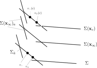
Figure 7. $v_{-}(c)$ and $v_{+}(c)$

Next we will prove that we can take a subsequence such that there exists

$$u_{\infty}:\Sigma({\bf x}_{\infty})\to X$$

satisfying

(7.30) $$\lim_{c\to\infty}u_{c}=u_{\infty},$$

in the following sense.

The spaces $\Sigma({\bf x}_{c})$ are submanifolds of the metric space $\widetilde{\mathcal{OB}}$, the total space of our universal family. This sequence of submanifolds $\Sigma({\bf x}_{c})$ converges to $\Sigma({\bf x}_{\infty})$ by Hausdorff distance (of subsets of $\widetilde{\mathcal{OB}}$). Let $\rho_{c}$ be the Hausdorff distance between them. (Note $\lim_{c\to\infty}\rho_{c}=0$.)

Now (7.30) means that

(7.31) $$\lim_{c\to\infty}\sup\{d_{X}(u_{c}(x),u_{\infty}(y))\mid(x,y)\in\Sigma({\bf x}_{c})\times\Sigma({\bf x}_{\infty}),\,\,d(x,y)\leq 2\rho_{c}\}=0.$$

(See Figure 8.)

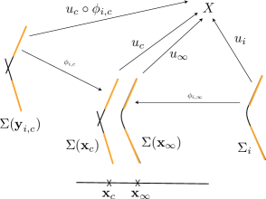
Figure 8. $\lim_{c\to\infty}u_{c}=u_{\infty}$

We now prove the existence of the limit $u_{\infty}$.

Item (2) above, Sublemmata 7.31, 7.32 and (7.28),(7.29) imply that, for $i=1,2$, there exists a unique isomorphism

(7.32) $$\phi_{i,\infty}:(\Sigma_{i},\vec{z}_{i}\cup\vec{w}_{i})\cong(\Sigma({\bf x}_{\infty}),\vec{z}({\bf x}_{\infty})\cup\vec{w}_{i}({\infty})).$$

We consider

$$\phi_{i,c}\circ\Phi_{i,{\bf y}_{i,c},\delta_{i}(c)}:\Sigma_{i}(\delta_{i}(c))\to\Sigma({\bf x}_{c})$$

and regard it as a map to $\widetilde{\mathcal{OB}}$.

Sublemma 7.34.

There exists $\phi_{i,\infty}$ such that

$$\lim_{c\to\infty}\phi_{i,c}\circ\Phi_{i,{\bf y}_{i,c},\delta_{i}(c)}=\phi_{i,\infty}.$$

Proof.

We consider the total space of the universal deformation of the stable marked nodal curve $(\Sigma_{i},\vec{z}_{i}\cup\vec{w}_{i})$. In this space the sequence $\vec{z}({\bf y}_{i,c})\cup\vec{w}({\bf y}_{i,c})$ converges to $\vec{z}_{i}\cup\vec{w}_{i}$. On the other hand, in the total space $\widetilde{\mathcal{OB}}$, the marked points $\vec{z}({\bf x}_{c})\cup\vec{w}_{i}(c)$ converges to $\vec{z}({\bf x}_{\infty})\cup\vec{w}_{i}({\infty})$. The sublemma is then an immediate consequence of (7.27), (7.32), the stability of $(\Sigma_{i},\vec{z}_{i}\cup\vec{w}_{i})$ and the fact that $\Phi_{i,{\bf y}_{i,c},\delta(c)}$ converges to the identity map. ∎

Item (1) above implies that

$$\lim_{c\to\infty}\sup\{d_{X}((u_{c}\circ\phi_{i,c}\circ\Phi_{i,{\bf y}_{i,c},\delta(c)})(z),u_{i}(z))\mid z\in\Sigma_{i}(\delta(c))\}=0,$$

and that $u_{c}\circ\phi_{i,c}\circ\Phi_{i,{\bf y}_{i,c},\delta(c)}$ is equicontinuous.

Item (3) above implies that the diameter of the image by $u_{c}\circ\phi_{i,c}$ of each connected component of $\Sigma_{i}({\bf y}_{i,c})\setminus{\rm Im}(\Phi_{i,{\bf y}_{i,c},\delta_{i}(c)})$ is smaller than $o(c)$.

Therefore we can take

$$u_{\infty}=u_{i}\circ(\phi_{i,\infty})^{-1}.$$

Note $u_{\infty}$ is independent of $i$ since it satisfies Formula (7.31).

We are now in the position to complete the proof of Proposition 7.28. By (7.31) we have

$$((\Sigma_{1},\vec{z}_{1}),u_{1})\overset{\phi_{\infty,1}}{\cong}((\Sigma({\bf x}_{\infty}),\vec{z}({\bf x}_{\infty})),u_{\infty})\overset{\phi_{\infty,2}^{-1}}{\cong}((\Sigma_{2},\vec{z}_{2}),u_{2}).$$

This contradicts to $[(\Sigma_{1},\vec{z}_{1}),u_{1}]\neq[(\Sigma_{2},\vec{z}_{2}),u_{2}]$. ∎

Remark 7.35.

In the proof of Proposition 7.28 we proved Hausdorff-ness directly. Alternatively we can proceed as follows. (See [FOOO14, Section 3], [FOOO11, Section 3], [FOOO5, Part 7] and etc. for the definition of Kuranishi structure and good coordiante system.) By Proposition 7.26 we find a Kuranishi chart at each point of the $G$-orbit of $[(\Sigma,\vec{z}),u]\in\mathcal{M}_{g,\ell}((X,J);\alpha)$. Using (the proof of) Proposition 7.36 we can show the existence of the coordinate change and obtain a Kuranishi structure on the $G$-orbit of $[(\Sigma,\vec{z}),u]\subset\mathcal{M}_{g,\ell}((X,J);\alpha)$. We take a good coordinate system compatible with it. (See [FOOO14, Section 11] etc. for the existence of such a good coordinate system.) Then by [FOOO7, Theorem 2.9] we can shrink this good coordinate system so that we obtain a Hausdorff space by gluing the Kuranishi charts which are members of the good coordinate system obtained by the above shrinking. This will become the Kuranishi neighborhood we look for.

The proof we gave here is self-contained and does not use the results of [FOOO7] or the existence theorem of compatible good coordinate system.

Let $({\mathfrak{W}}^{(i)},\vec{\mathcal{N}}_{(i)})$ be strong stabilization data at $(((\Sigma_{i},\vec{z}_{i}),u_{i});\epsilon,{\mathfrak{W}}^{(i)})$, for $i=1,2$. We defined $V(((\Sigma_{i},\vec{z}_{i}),u_{i});\epsilon,({\mathfrak{W}}^{(i)},\vec{\mathcal{N}}^{(i)}))$ in Definition 7.22.

Proposition 7.36.

If $\epsilon$ is smaller than a positive number depending on $n$ and $\epsilon^{\prime}$ is smaller than a positive number depending on $n$ and $\epsilon$, then the embedding (7.25) becomes a $C^{n}$ embedding with respect to the smooth structure as open subsets of $V(((\Sigma_{1},\vec{z}_{1}),u_{1});\epsilon,({\mathfrak{W}}^{(1)},\vec{\mathcal{N}}^{(1)}))/\mathcal{G}_{1}$ and $V(((\Sigma_{2},\vec{z}_{2}),u_{2});\epsilon^{\prime},({\mathfrak{W}}^{(2)},\vec{\mathcal{N}}^{(2)}))/\mathcal{G}_{2}$. Here $\mathcal{G}_{2}=\mathcal{G}((\Sigma_{2},\vec{z}_{2}),u_{2})$, the group of automorphisms of $((\Sigma_{2},\vec{z}_{2}),u_{2})$.

This is proved in [FOOO6, Part 4] and [FOOO12, Section 10]. We repeat the proof in Subsection 7.5 for the sake of completeness.

We remark that by definition the restriction of the bundle $E(((\Sigma_{1},\vec{z}_{1}),u_{1});\epsilon,({\mathfrak{W}}^{(1)},\vec{\mathcal{N}}_{1}))$ to $\mathcal{U}(\epsilon^{\prime};(\Sigma_{2},\vec{z}_{2}),u_{2},{\mathfrak{W}}^{(2)})$ is canonically isomorphic to the restriction of the bundle $E(((\Sigma_{2},\vec{z}_{2}),u_{2});\epsilon^{\prime},({\mathfrak{W}}^{(2)},\vec{\mathcal{N}}_{2}))$.

Lemma 7.37.

This canonical isomorphism preserves the $C^{n}$ structure of vector bundles.

The proof is also in Subsection 7.5.

By Proposition 7.36 and Lemma 7.37 we can glue $C^{n}$ structures to obtain a $C^{n}$ structure on $U(((\Sigma,\vec{z}),u);\epsilon_{2})$ and on the vector bundle $E(((\Sigma,\vec{z}),u);\epsilon_{2})$. (The later is obtained by gluing $E((\Sigma_{1},\vec{z}_{1}),u_{1});\epsilon,({\mathfrak{W}}^{(1)},\vec{\mathcal{N}}_{1}))$.) We can then glue the Kuranishi map $s$ and parametrization map $\psi$ defined for various $((\Sigma_{1},\vec{z}_{1}),u_{1});\epsilon,({\mathfrak{W}}^{(1)},\vec{\mathcal{N}}^{(1)}))$ in Proposition 7.26.

Thus we obtain a Kuranishi chart

(7.33) $$(U(((\Sigma,\vec{z}),u);\epsilon_{2}),E(((\Sigma,\vec{z}),u);\epsilon_{2}),s,\psi),$$

of $C^{n}$ class for any $n$.

Lemma 7.38.

The Kuranishi chart (7.33) is of $C^{\infty}$ class.

This is proved in [FOOO6, Section 26], [FOOO12, Section 12]. We repeat the proof in Subsection 7.6 for the sake of completeness.

We finally prove:

Lemma 7.39.

The Kuranishi chart (7.33) is $G$-equivariant.

Proof.

Let $((\Sigma_{1},\vec{z}_{1}),u_{1})\in U(((\Sigma,\vec{z}),u);\epsilon_{2})$. We take its strong stabilization data $({\mathfrak{W}},\vec{\mathcal{N}})$ as in Definition 7.5. Note all the data in ${\mathfrak{W}}$ are independent of $u_{1}$. Therefore we can define $g{\mathfrak{W}}$ for $((\Sigma_{1},\vec{z}_{1}),gu_{1})$ so that it is the same as ${\mathfrak{W}}$. We replace $\mathcal{N}_{i}$ by $g\mathcal{N}_{i}$ to define $g\vec{\mathcal{N}}$

Then there exists an isomorphism

$$V(((\Sigma_{1},\vec{z}_{1}),u_{1});({\mathfrak{W}},\vec{\mathcal{N}}))\cong V(((\Sigma_{1},\vec{z}_{1}),gu_{1});(g{\mathfrak{W}},g\vec{\mathcal{N}}))$$

sending $({\bf v},{\bf x})$ to $(g_{*}{\bf v},{\bf x})$. Note ${\bf v}$ is an element of ${\rm Ker}^{+}D_{u_{1}}\overline{\partial}$ defined in (7.16). Therefore $g_{*}{\bf v}$ is an element of ${\rm Ker}^{+}D_{gu_{1}}\overline{\partial}$. This is because

$$g_{*}E((\Sigma_{1},\vec{z}_{1}),u_{1})=E((\Sigma_{1},\vec{z}_{1}),gu_{1}).$$

(Lemma 6.12.)

Furthermore, the gluing construction of $u_{{\bf v},{\bf x}}$ is invariant of $G$ action. Nameley:

$$gu_{{\bf v},{\bf x}}=u_{g{\bf v},{\bf x}}.$$

Therefore $((\Sigma^{\prime},\vec{z}^{\,\prime}),u^{\prime})\mapsto((\Sigma^{\prime},\vec{z}^{\,\prime}),gu^{\prime})$ defines a smooth map from a neighborhood of $[(\Sigma_{1},\vec{z}_{1}),u_{1}]$ in $U((\Sigma,\vec{z}),u);\epsilon_{2})$ to a neighborhood of $[(\Sigma_{1},\vec{z}_{1}),gu_{1}]$ in $U(((\Sigma,\vec{z}),u);\epsilon_{2})$. Thus $G$ action is a smooth action on $U(((\Sigma,\vec{z}),u);\epsilon_{2})$.

Smoothness of the $G$-action on the obstruction bundle can be proved in the same way. $G$-equivariance of $s$ and $\psi$ is obvious from the definition. ∎

The proof of Proposition 6.15 except the parts deferred to Subsections 7.4, 7.5 and 7.6 is now complete. ∎

7.4. Exponential decay estimate of obstruction bundle

In this section we prove Proposition 7.14.

We consider the set $\mathcal{V}_{(1)}=\mathcal{V}_{1,0}\times\mathcal{V}_{1,1}$. It is a set of $(\vec{x},\vec{\rho})$ where $\vec{\rho}\in\mathcal{V}_{1,1}$ is the parameter to smooth the node of $(\Sigma_{1},\vec{z}_{1}\cup\vec{w}_{1})$ and $\vec{x}=(x_{a})_{a\in\mathcal{A}_{s}}\in\mathcal{V}_{1,0}$ is the parameter to deform the complex structure of each irreducible component of $(\Sigma_{1},\vec{z}_{1}\cup\vec{w}_{1})$. It comes with the universal family $\pi_{(1)}:\mathcal{C}_{(1)}\to\mathcal{V}_{(1)}$. (See (7.7).) For each ${\bf x}\in\mathcal{V}_{(1)}$ its fiber together with marked points is written as $(\Sigma_{1}({\bf x}),\vec{z}_{1}({\bf x})\cup\vec{w}_{1}({\bf x}))$.

We assumed that $((\Sigma_{1},\vec{z}_{1}),u_{1})$ is $G$-$\epsilon_{2}$-close to $((\Sigma,\vec{z}),u)$. We consider the universal family of deformation of $(\Sigma,\vec{z})$. Suppose that the universal family is obtained from $\pi:\mathcal{C}\to\mathcal{V}$, which is a holomorphic map between complex manifolds and has nodal curves as fibers, by Construction 2.17. (See the proof of Theorem 3.5 in Subsection 3.2.)

Lemma 7.40.

There exist holomorphic maps

$$\tilde{\psi}:\mathcal{C}_{(1)}\to\mathcal{C},\qquad\psi:\mathcal{V}_{(1)}\to\mathcal{V}$$

with the following properties.

1. The next diagram commutes

   (7.34) $$\begin{CD}\mathcal{C}_{(1)}@ >{\tilde{\psi}}>>\mathcal{C},\\ @ VV{\pi_{(1)}}V@ VV{\pi}V\\ \mathcal{V}_{(1)}@ >{\psi}>>\mathcal{V},\end{CD}$$

   and is cartesian.

2. The next diagram commutes for $j=1,\dots,\ell$.

   (7.35) $$\begin{CD}\mathcal{C}_{(1)}@ >{\tilde{\psi}}>>\mathcal{C},\\ @ AA{\mathfrak{T}_{j}}A@ AA{\mathfrak{t}_{j}}A\\ \mathcal{V}_{(1)}@ >{\psi}>>\mathcal{V},\end{CD}$$

   Here $\mathfrak{T}_{j}$ and $\mathfrak{t}_{j}$ are sections which assign the marked points.

3. $\tilde{\psi}$ and $\psi$ are $\mathcal{G}_{1}$ equivariant.

Proof.

By forgetting $\mathfrak{t}_{j}$ for $j=\ell+1,\dots,\ell+k$ (namely the marked points $\vec{w}({\bf x})$), the family $\mathcal{C}_{(1)}\to\mathcal{V}_{(1)}$ becomes a deformation of $(\Sigma_{1},\vec{z}_{1})$. Therefore in case $(\Sigma_{1},\vec{z}_{1})=(\Sigma,\vec{z})$ the lemma is a consequence of the universality of $\pi:\mathcal{C}\to\mathcal{V}$.

The general case can be reduced to the case $(\Sigma_{1},\vec{z}_{1})=(\Sigma,\vec{z})$ by using Sublemma 3.20. ∎

Remark 7.41.

We use the universality in Theorem 3.5 here. We remark that here the universality we use is one for the complex analytic family. A similar universality for $C^{\infty}$ family also holds. This is a part of classical theory by Kodaira-Spencer in the case of non-singular curves. In the general case where curves are nodal, one can prove it, for example, by working out the study of a neighborhood of a point of Deligne-Mumford moduli space that corresponds to a nodal curve by an analytic method of gluing. (See for example [FOOO10, Section 25] and compare [FOOO8, Remark 8.36].)

We are given a map $u_{1}:\Sigma_{1}\to X$. Note that $\Sigma_{1}=\Sigma({\bf x}_{1})$. We regard it as a subset $\pi^{-1}({\bf x}_{1})$ of the total space $\mathcal{C}$ of the universal family and extends it to a smooth map $F$ from a neighborhood of $\pi^{-1}({\bf x}_{1})$ in $\mathcal{C}$. Let $F_{1}=F\circ\tilde{\psi}$ be its composition with $\tilde{\psi}$. For ${\bf x}\in\mathcal{V}_{(1)}$ such that $\psi({\bf x})$ is close to ${\bf x}_{1}$, we denote the restriction of $F_{1}$ to $\pi^{-1}({\bf x})$ by $u_{{\bf x}}:\Sigma_{1}({\bf x})\to X$.

Definition 7.42.

For $\epsilon_{4}>0$, we define $\mathcal{W}(\epsilon_{4})$ as follows:

(7.36) $$\mathcal{W}(\epsilon_{4})=\bigcup_{{\bf x}\in\mathcal{V}_{(1)}}\mathcal{W}(\epsilon_{4};\psi({\bf x}),(\tilde{\psi}|_{\Sigma_{1}({\bf x})})^{-1};((\Sigma_{1}({\bf x}),\vec{z}_{1}({\bf x})),u_{{\bf x}}))\times\{{\bf x}\}.$$

See Definition 6.1 for the notation appearing in the right hand side. Note that $(\tilde{\psi}|_{\Sigma_{1}({\bf x})})^{-1}:\Sigma(\psi({\bf x}))\to\Sigma_{1}({\bf x})$ is an isomorphism which plays the role of $\phi_{0}$ in Definition 6.1.

We define ${\rm Pro}:\mathcal{W}(\epsilon_{4})\to\mathcal{V}_{(1)}$ by assigning $\bf x$ to all the elements of the subset $\mathcal{W}(\epsilon_{4};\psi({\bf x}),(\tilde{\psi}|_{\Sigma_{1}({\bf x})})^{-1};((\Sigma_{1}({\bf x}),\vec{z}_{1}({\bf x})),u_{{\bf x}}))\times\{{\bf x}\}$.

In a similar way as Definition 6.7 we define a right $\widehat{\mathcal{G}}_{c}$ action on $\mathcal{W}(\epsilon_{4})$ as follows. Let $(\varphi,g,{\bf x})\in\mathcal{W}(\epsilon_{4})$ and $\upsilon=(\gamma,h)\in\widehat{\mathcal{G}}_{c}$. We have ${\rm Pr}_{t}(\varphi)=\psi({\bf x})$. We put $\overline{\bf y}={\rm Pr}_{s}(\varphi)$. Then $\gamma\in\mathcal{MOR}$ induces an isomomrphism $\gamma_{*}:(\Sigma(\overline{\bf y}),\vec{z}(\overline{\bf y}))\cong(\Sigma(\psi({\bf x})),\vec{z}(\psi({\bf x}))$. We put $\vec{w}^{\prime}=\gamma_{*}^{-1}(\tilde{\psi}|_{\Sigma_{1}({\bf x})}(\vec{w}(\bf x)))$. There exists a unique ${\bf y}$ such that

$$(\Sigma(\overline{\bf y}),\vec{z}(\overline{\bf y}),\vec{w}^{\prime})\cong(\Sigma_{1}({\bf y}),\vec{z}_{1}({\bf y}),\vec{w}_{1}({\bf y})).$$

In particular $\psi({\bf y})=\overline{\bf y}$. We now put

$$\upsilon(\varphi,g,{\bf x})=(\varphi\circ\gamma_{*},gh,{\bf y}).$$

The $\widehat{\mathcal{G}}_{c}$ action is free and smooth. We denote

$$\overline{\mathcal{W}}(\epsilon_{4})=\mathcal{W}(\epsilon_{4})/\widehat{\mathcal{G}}_{c}.$$

${\rm Pro}$ induces a map $\overline{\rm Pro}:\overline{\mathcal{W}}(\epsilon_{4})\to\mathcal{V}_{(1)}$.

Lemma 7.43.

$\mathcal{W}(\epsilon_{4})$ has a structure of complex manifold and $\overline{\rm Pro}$ is a submersion.

Proof.

The proof is the same as the proof of Lemma 6.2, using the fact that ${\rm Pr}_{t}$ is a submersion. ∎

Let $U^{\prime}(\epsilon)$ be the $\epsilon$ neighborhood of $u_{1}|_{\Sigma_{1}(\delta)}$ in $L^{2}_{m+1}$ norm (as in Proposition 7.14). (By taking $\epsilon$ small we may regard $U^{\prime}(\epsilon)$ as an open subset of an appropriate Hilbert space (that is, $L^{2}_{m+1}$ space).)

Definition 7.44.

We define a function

$${\rm meandist}:\mathcal{W}(\epsilon_{4})\times U^{\prime}(\epsilon)\to{\mathbb{R}}$$

as follows. Let $(\varphi,g,{\bf x},\hat{u}^{\prime})\in\mathcal{W}(\epsilon_{4};\psi({\bf x}),(\tilde{\psi}|_{\Sigma_{1}({\bf x})})^{-1};((\Sigma_{1}({\bf x}),\vec{z}_{1}({\bf x})),u_{{\bf x}}))\times\{{\bf x}\}\times U^{\prime}(\epsilon)$. We slightly modify (6.1) to set:

(7.37) $${\rm meandist}(\varphi,g,{\bf x},\hat{u}^{\prime})$$

$$=\int_{z\in\Sigma(\sigma)}\chi(z)\,\,d_{X}^{2}((\hat{u}^{\prime}\circ\Phi_{1,{\bf x},\delta}^{-1}\circ(\tilde{\psi}|_{\Sigma_{1}({\bf x})})^{-1}\circ\varphi\circ\Phi_{\overline{\bf x}^{\prime},\sigma})(z),gu(z))\,\,\Omega_{\Sigma},$$

where $\overline{\bf x}^{\prime}={\rm Pr}_{s}(\varphi)$. Note that the map $\hat{u}^{\prime}\circ\Phi_{1,{\bf x},\delta}^{-1}\circ(\tilde{\psi}|_{\Sigma_{1}({\bf x})})^{-1}\circ\varphi\circ\Phi_{\overline{\bf x}^{\prime},\sigma}$ is a composition

$$\Sigma(\sigma)\longrightarrow\Sigma(\overline{\bf x}^{\prime})(\sigma)\longrightarrow\Sigma(\psi({\bf x}))(\sigma)\longrightarrow\Sigma_{1}({\bf x})(\delta)\longrightarrow\Sigma_{1}(\delta)\longrightarrow X,$$

which is defined if $\delta$ is small compared with $\sigma$.

It is $\widehat{\mathcal{G}}_{c}$ invariant and induces

$$\overline{\rm meandist}:\overline{\mathcal{W}}(\epsilon_{4})\times U^{\prime}(\epsilon)\to{\mathbb{R}}.$$

Lemma 7.45.

We assume $\epsilon_{4}$ and $\epsilon$ are sufficiently small. Then the functions ${\rm meandist}$ and $\overline{\rm meandist}$ are smooth functions. The restriction of $\overline{\rm meandist}$ to the fibers of $\overline{\rm Pro}:\overline{\mathcal{W}}(\epsilon_{4})\to\mathcal{V}_{(1)}$ are strictly convex. Moreover the restriction of $\overline{\rm meandist}$ to the fibers of $\overline{\rm Pro}$ attains its minimum at a unique point.

Proof.

The smoothness of ${\rm meandist}$ and $\overline{\rm meandist}$ is immediate from (6.1). To show strict convexity it suffices to consider the case $\psi({\bf x})={\bf x}_{1}$, that is, $\Sigma_{1}({\bf x})=\Sigma_{1}$. (This is because we can then shrink $\mathcal{V}_{(1)}$ and use the fact that strict convexity is an open property.) This case is proved as Proposition 6.8. The uniqueness of minimum is Lemma 6.9. ∎

We remark that ${\rm Pro}^{-1}({\bf x})\subset{\mathcal{W}}(\epsilon_{4})$ is identified with an open subset $\mathcal{MOR}\times G$, which is nothing but

$$\mathcal{W}(\epsilon_{4};\psi({\bf x}),(\tilde{\psi}|_{\Sigma_{1}({\bf x})})^{-1};((\Sigma_{1}({\bf x}),\vec{z}_{1}({\bf x})),u_{{\bf x}})).$$

Lemma 7.46.

There exists a smooth map

$$\overline{\Phi}:U^{\prime}(\epsilon)\times\mathcal{V}_{(1)}\to(\mathcal{MOR}\times G)/\widehat{\mathcal{G}}_{c}$$

such that for each $\hat{u}^{\prime}\in U^{\prime}(\epsilon)$, ${\bf x}\in\mathcal{V}_{(1)}$, the element $\overline{\Phi}(\hat{u}^{\prime},{\bf x})$ is contained in the subset $\overline{\mathcal{W}}(\epsilon_{4})$ of $(\mathcal{MOR}\times G)/\widehat{\mathcal{G}}_{c}$ and $\overline{\Phi}(\hat{u}^{\prime},{\bf x})$ is the unique point on $\overline{\rm Pro}^{-1}({\bf x})$ where $\overline{\rm meandist}$ attains its minimum.

Proof.

This is a consequence of Lemma 7.45 and Lemma 8.9. ∎

Remark 7.47.

We remark that elements of $U^{\prime}(\epsilon)$ are $L^{2}_{m+1}$ maps. Nevertheless our map $\overline{\Phi}$ is smooth. This is because the function ${\rm meansdist}$ is defined by using integration and so is a smooth function on the space of $L^{2}_{m+1}$ maps.

The way we define $\overline{\rm meandist}$ in this subsection is slightly different from the way we defined it in Section 6. However the local minimum is assumed at the same point. More precisely we can prove the next lemma.

To state the lemma we need notations. Suppose $((\Sigma^{\prime},\vec{z}^{\prime}),u^{\prime})$ is $G$-$\epsilon_{1}$-close to $((\Sigma,\vec{z}),u)$. We take $\overline{\bf x}\in\mathcal{V}$ such that there exists an isomorphism

$$\phi_{0}:(\Sigma(\overline{\bf x}),\vec{z}(\overline{\bf x}))\cong(\Sigma^{\prime},\vec{z}^{\prime}).$$

Then Definition 6.4 defines

$$\overline{\rm meandist}^{\S\ref{sec:main}}:\mathcal{W}(\epsilon_{4};\overline{\bf x},\phi_{0};((\Sigma^{\prime},\vec{z}^{\prime}),u^{\prime}))/\widehat{\mathcal{G}}_{c}\to{\mathbb{R}}$$

We assume that $\overline{{\bf x}}$ is in a small neighborhood of ${\bf x}_{1}$ and take ${\bf x}\in\mathcal{V}_{(1)}$ such that $\psi({\bf x})=\overline{{\bf x}}$. We then put

(7.38) $$\hat{u}^{\prime}=u^{\prime}\circ\phi_{0}\circ\tilde{\psi}|_{\Sigma_{1}({\bf x})}\circ\Phi_{1,{\bf x},\delta}:\Sigma_{1}(\delta)\to X.$$

Note that this is a composition

$$\Sigma_{1}(\delta)\longrightarrow\Sigma_{1}({\bf x})(\delta)\longrightarrow\Sigma(\psi({\bf x}))\longrightarrow\Sigma^{\prime}\longrightarrow X.$$

We assume $\hat{u}^{\prime}\in U^{\prime}(\epsilon)$. Then, by Definition 7.44, we obtain a function:

$$\overline{\rm meandist}^{\S\ref{sec:decay}}:\mathcal{W}(\epsilon_{4};\psi({\bf x}),(\tilde{\psi}|_{\Sigma_{1}({\bf x})})^{-1};((\Sigma_{1}({\bf x}),\vec{z}_{1}({\bf x})),u_{{\bf x}}))/\widehat{\mathcal{G}}_{c}\to{\mathbb{R}}$$

which is nothing but

$$[\varphi,g]\mapsto\overline{\rm meandist}(\varphi,g,{\bf x},\hat{u}^{\prime})$$

where $\overline{\rm meandist}$ in the right hand side is one defined in Definition 7.44.

Lemma 7.48.

We can shrink $\mathcal{V}_{(1)}$ and replace $\epsilon$ by a smaller positive number so that the next two conditions are equicalent.

1. $[\varphi,g]\in\mathcal{W}(\epsilon_{4};\overline{\bf x},\phi;((\Sigma^{\prime},\vec{z}^{\prime}),u^{\prime}))/\widehat{\mathcal{G}}_{c}$ and $\overline{\rm meandist}^{\S\ref{sec:main}}$ takes the minimum there.

2. $[\varphi,g]\in\mathcal{W}(\epsilon_{4};\psi({\bf x}),(\tilde{\psi}|_{\Sigma_{1}({\bf x})})^{-1};((\Sigma_{1}({\bf x}),\vec{z}_{1}({\bf x})),u_{{\bf x}}))/\widehat{\mathcal{G}}_{c}$ and $\overline{\rm meandist}^{\S\ref{sec:decay}}$ takes the minimum there.

Proof.

Comparing formulas (7.38), (7.37) and (6.1) it is easy to see that $\overline{\rm meandist}^{\S\ref{sec:main}}=\overline{\rm meandist}^{\S\ref{sec:decay}}$ when both are defined. (We remark that the domains of the both functions are quotient of open subsets of $\mathcal{MOR}\times G$ by $\widehat{\mathcal{G}}_{c}$. So the intersection of the domains makes sense.) In fact

$$\hat{u}^{\prime}\circ\Phi_{1,{\bf x},\delta}^{-1}\circ(\tilde{\psi}|_{\Sigma_{1}({\bf x})})^{-1}\circ\varphi\circ\Phi_{{\bf x}^{\prime},\sigma}$$

$$=u^{\prime}\circ\phi_{0}\circ\tilde{\psi}|_{\Sigma_{1}({\bf x})}\circ\Phi_{1,{\bf x},\delta}^{-1}\circ\Phi_{1,{\bf x},\delta}\circ(\tilde{\psi}|_{\Sigma_{1}({\bf x})})^{-1}\circ\varphi\circ\Phi_{{\bf x}^{\prime},\sigma}$$

$$=u^{\prime}\circ\phi_{0}\circ\varphi\circ\Phi_{{\bf x}^{\prime},\sigma}.$$

In the case when $\psi({\bf x})={\bf x}_{1}$ and $u^{\prime}=u_{1}$, the domain also coincides. So the lemma holds in that case. We can shrink $\mathcal{V}_{(1)}$ and replace $\epsilon$ by a smaller positive number and use the strict covexity of $\overline{\rm meandist}^{\S\ref{sec:main}}$ and of $\overline{\rm meandist}^{\S\ref{sec:decay}}$ to show the general case. ∎

Proposition 7.14 is a consequence of Lemmas 7.46 and 7.48 and a straight forward computation based on the definition. For completeness’ sake we provide the detail of its proof below.

Let $\mathcal{V}_{(1)}(\epsilon)$ be the $\epsilon$ neighborhood of $0$ in $\mathcal{V}_{(1)}$ as in Proposition 7.14. If $\epsilon$ is small we can find a lift

$$\Phi:U^{\prime}(\epsilon)\times\mathcal{V}_{(1)}(\epsilon)\to\mathcal{MOR}\times G$$

of $\overline{\Phi}$. We put

(7.39) $$\Phi(\hat{u}^{\prime},{\bf x})=(\varphi(\hat{u}^{\prime},{\bf x}),g(\hat{u}^{\prime},{\bf x})).$$

Thus

$$\varphi(\cdot):U^{\prime}(\epsilon)\times\mathcal{V}_{(1)}(\epsilon)\to\mathcal{MOR},\quad g(\cdot):U^{\prime}(\epsilon)\times\mathcal{V}_{(1)}(\epsilon)\to G,$$

are smooth maps (from a Hilbert space to finite dimensional manifolds).

We may take our lift $g(\cdot):U^{\prime}(\epsilon)\times\mathcal{V}_{(1)}(\epsilon)\to G$ so that its image lies in a neighborhood of $g_{1}$. We denote by $U_{G}(g_{1})$ this neighborhood.

We calculate the finite dimensional subspace $E(\hat{u}^{\prime},{\bf x})$ using local coordinate. We cover $\Sigma(\delta)$ by a sufficiently small open sets $W_{\sigma}$.

$$\Sigma(\delta)\subset\bigcup_{\sigma\in\mathcal{S}}W_{\sigma}.$$

We will specify how small $W_{\sigma}$ is later. We fix a complex coordinate of $W_{\sigma}$ and denote it by $z_{\sigma}$.

We first assume the following:

Assumption 7.49.

For each $\sigma$ there exists a convex open subset $\Omega_{\sigma}$ of $X$ in one chart such that the following holds for $\hat{u}^{\prime}\in U^{\prime}(\epsilon)$, ${\bf x}_{1}\in V_{(1)}$.

1. Note $(\Sigma_{1},\vec{z}_{1})=(\Sigma({\bf x}_{1}),\vec{z}({\bf x}_{1}))$. We have $\Phi_{{\bf x}_{1},\delta}:\Sigma(\delta)\to\Sigma_{1}.$ We require

   $$u_{1}(\Phi_{{\bf x}_{1},\delta}(W_{\sigma}))\subset\Omega_{\sigma}.$$

2. We also require

   $$\hat{u}^{\prime}(\Phi_{{\bf x}_{1},\delta}(W_{\sigma}))\subset\Omega_{\sigma}.$$

3. We also require

   $$gu(W_{\sigma})\subset\Omega_{\sigma},$$

   for $g\in U_{G}(g_{1})$.

Note that if the diameter of $W_{\sigma}$ is small and $\epsilon$, $\epsilon_{4}$ are small then the the diameter of the union of $u_{1}(\Phi_{{\bf x}_{1},\delta}(W_{\sigma}))$, $\hat{u}^{\prime}(\Phi_{{\bf x}_{1},\delta}(W_{\sigma}))$ and $g_{1}u(W_{\sigma})$ is small. In fact $\hat{u}^{\prime}$ is close to $u_{1}$ and $u_{1}\circ\Phi_{{\bf x}_{1},\delta}$ is close to $g_{1}u$. Therefore we may assume the existence of $\Omega_{\sigma}$.

Let $\partial_{\sigma}^{1},\dots,\partial_{\sigma}^{d}$ be a local (complex) frame of the complex tangent bundle $TX$ on $\Omega_{\sigma}$.

Definition 7.50.

We define a (complex) matrix valued smooth function $({\rm Pal}^{i}_{j}(p,q))_{i,j=1}^{\dim X}$ on $\Omega_{\sigma}^{2}$ with the following properties. Let $p,q\in\Omega_{\sigma}^{2}$. We take the shortest geodesic $\gamma$ joining $p$ to $q$. Using local frames $\partial_{\sigma}^{i}$ at $p,q$ and the parallel transportation (with respect to an appropriate hermitian connection)

$${\rm Pal}_{p}^{q}:T_{p}X\to T_{q}X$$

along $\gamma$, we define

(7.40) $${\rm Pal}_{p}^{q}(\partial_{\sigma}^{j})=\sum_{i}{\rm Pal}^{i}_{j}(p,q)\partial_{\sigma}^{i}.$$

Other than parallel transportation, the differentials of $\Psi$ (See (6.8).) and of $\Phi_{1,{\bf x},\delta}$ (See (7.11).) appear in the definition of $E(\hat{u}^{\prime},{\bf x})$. We write them by local coordinate below.

Let $\hat{u}^{\prime}\in U^{\prime}(\epsilon)$, ${\bf x}\in\mathcal{V}_{(1)}(\epsilon)$. We put

$$\overline{\bf y}=\overline{\bf y}(\hat{u}^{\prime},{\bf x})={\rm Pr}_{s}(\varphi(\hat{u}^{\prime},{\bf x})),$$

where $\varphi$ is defined by (7.39). (6.8) in this case becomes:

(7.41) $$\Psi_{\hat{u}^{\prime},{\bf x}}=(\Phi_{\overline{\bf y}(\hat{u}^{\prime},{\bf x}),\delta})^{-1}\circ(\varphi(\hat{u}^{\prime},{\bf x}))^{-1}\circ\tilde{\psi}|_{\Sigma_{1}({\bf x}))}:\Sigma_{1}({\bf x})(\delta^{\prime})\to\Sigma(\delta).$$

Note that $\phi_{0}=(\tilde{\psi}|_{\Sigma_{1}({\bf x}))})^{-1}$ in our case as we mentioned in Definition 7.42. (7.41) is a composition

$$\Sigma_{1}({\bf x})(\delta^{\prime})\longrightarrow\Sigma(\psi({\bf x}))(\delta)\longrightarrow\Sigma(\overline{\bf y})(\delta)\longrightarrow\Sigma(\delta).$$

We compose it with $\Phi_{1,{\bf x},\delta^{\prime}}$ to obtain

(7.42) $$\Psi_{\hat{u}^{\prime},{\bf x}}\circ\Phi_{1,{\bf x},\delta^{\prime}}:\Sigma_{1}(\delta^{\prime})\to\Sigma(\delta).$$

Note the source and the target is independent of $(\hat{u}^{\prime},{\bf x})$. This family of maps depends smoothly on $\hat{u}^{\prime},{\bf x}$.

Assumption 7.51.

There exists a coordinate chart $W_{1,\sigma}$ of $\Sigma_{1}$ independent of $\hat{u}^{\prime},{\bf x}$ such that

$$(\Psi_{\hat{u}^{\prime},{\bf x}}\circ\Phi_{1,{\bf x},\delta})(W_{1,\sigma})\supset W_{\sigma}.$$

Moreover

$$\Psi_{\hat{u}^{\prime},{\bf x}}(\Phi_{1,{\bf x},\delta}(W_{1,\sigma}))$$

is contained in a coordinate chart $W^{+}_{\sigma}$ containing $W_{\sigma}$, to which the coordinate $z_{\sigma}$ extends.

By choosing $\epsilon$ small and $W_{\sigma}$ small we can assume that such $W_{1,\sigma}$ exists. We fix a complex coordinate $z_{1,\sigma}$ of $W_{1,\sigma}$.

Using complex linear part of the differential of $\Psi_{\hat{u}^{\prime},{\bf x}}$ we obtain a bundle map

$$d^{h}\Psi_{\hat{u}^{\prime},{\bf x}}:\Lambda^{01}\Sigma(\delta)\to\Lambda^{01}\Sigma_{1}({\bf x}).$$

We also have

$$d^{h}\Phi_{1,{\bf x},\delta}:\Lambda^{01}\Sigma_{1}({\bf x})\to\Lambda^{01}\Sigma_{1}.$$

We denote the composition of them by

$$d^{h}\Phi_{1,{\bf x},\delta}\circ d^{h}\Psi_{\hat{u}^{\prime},{\bf x}}:\Lambda^{01}\Sigma(\delta)\to\Lambda^{01}\Sigma_{1}.$$

This is a bundle map which covers the (local) inverse of (7.42).

Lemma 7.52.

There exists a smooth function

$$\mathfrak{f}:U^{\prime}(\epsilon)\times\mathcal{V}_{(1)}(\epsilon)\times W_{1,\delta}\to{\mathbb{C}}$$

such that

(7.43) $$(d^{h}\Phi_{1,{\bf x},\delta}\circ d^{h}\Psi_{\hat{u}^{\prime},{\bf x}})(d\overline{z}_{\sigma})(w)=\mathfrak{f}(\hat{u}^{\prime},{\bf x},w)d\overline{z}_{1,\sigma}(w),$$

where $w\in W_{1,\delta}$.

Proof.

This is immediate from smooth dependence of $\Psi_{\hat{u}^{\prime},{\bf x}}$ and $\Phi_{1,{\bf x},\delta}$ on $\hat{u}^{\prime},{\bf x}$. ∎

We next write $G$ action by local coordinate. We recall that $U_{G}(g_{1})$ is a neighborhood of $g_{1}$ in $G$ such that the image of the map $g(\cdot)$ is contained in $U_{G}(g_{1})$.

Assumption 7.53.

We take $\Omega_{\sigma}$ so that there exist coordinate neighborhoods $\Omega^{0}_{\sigma}\subset\Omega^{+}_{\sigma}$ such that

$$\Omega^{0}_{\sigma}\subset g^{-1}\Omega_{\sigma}\subset\Omega^{+}_{\sigma},\qquad u(W_{\sigma})\subset\Omega^{0}_{\sigma}.$$

for any $g\in U_{G}(g_{1})$.

We can find such $\Omega^{0}_{\sigma}$, $\Omega^{+}_{\sigma}$ by taking $\epsilon$ sufficiently small. (Note that $g_{1}u$ is close to $\hat{u}^{\prime}\circ\Phi_{{\bf x}_{1},\delta}$.)

Let $\partial_{\sigma,0}^{i}$, $i=1,\dots,d$, be a local frame of the complex tangent bundle $TX$ on $\Omega^{+}_{\sigma}$.

Lemma 7.54.

There exists a matrix valued smooth function $(G(\hat{u}^{\prime},{\bf x},p)_{i}^{j})_{i,j=1}^{\dim X}$ on $U^{\prime}(\epsilon)\times\mathcal{V}_{(1)}(\epsilon)\times\Omega_{\sigma}$ such that

(7.44) $$\left(dg(\hat{u}^{\prime},{\bf x})(\partial_{\sigma,0}^{i})\right)(p)=\sum_{j}G(\hat{u}^{\prime},{\bf x},p)_{i}^{j}\partial_{\sigma}^{j}(p).$$

The map $dg(\hat{u}^{\prime},{\bf x})$ is the differential of the map defined by $g(\hat{u}^{\prime},{\bf x})\in G$ action.

Note $G(\cdot)_{i}^{j}:U^{\prime}(\epsilon)\times\mathcal{V}_{(1)}(\epsilon)\times\Omega_{\sigma}\to{\mathbb{C}}$ is a map from the product of Hilbert space and a finite dimensional manifold to the complex plane.

Proof.

The proof is immediate from the smoothness of $(\hat{u}^{\prime},{\bf x})\mapsto g(\hat{u}^{\prime},{\bf x})$, that is Lemma 7.46 and (7.39). ∎

We now write the map

$$E((\Sigma,\vec{z}),u)\to C^{\infty}(\Sigma_{1};u_{1}^{*}TX\otimes\Lambda^{01})$$

which we use to define

$$E(\hat{u}^{\prime},{\bf x})\subset C^{\infty}(\Sigma_{1};u_{1}^{*}TX\otimes\Lambda^{01})$$

explicitly using smooth functions appearing in (7.40), (7.43), (7.44) etc..

Let

$$e\in C^{\infty}(W_{\sigma};u^{*}TX\otimes\Lambda^{01})$$

has compact support. We write

(7.45) $$e=\sum_{i}e^{i}\partial_{\sigma,0}^{i}\otimes d\overline{z}_{\sigma}.$$

Here $e^{i}$ is a smooth function on $W_{\sigma}$. By (7.44) we have

(7.46) $$(g(\hat{u}^{\prime},{\bf x})_{*}(e))(w)=\sum_{i,j}G(\hat{u}^{\prime},{\bf x},w)_{i}^{j}e^{i}(w)\partial_{\sigma}^{j},$$

for $w\in W_{\sigma}$. Now we apply the maps

$$I_{{\bf x}_{0},\phi_{0};((\Sigma^{\prime},\vec{z}^{\,\prime}),u^{\prime})}:C^{\infty}(K;(gu)^{*}TX\otimes\Lambda^{01})\to L^{2}_{m+1}(\Sigma^{\prime}(\delta);(u^{\prime})^{*}TX\otimes\Lambda^{01})$$

and

$$I_{\hat{u}^{\prime},{\bf x}}:L^{2}_{m+1}(\Sigma_{1}({\bf x})(\delta);(u^{\prime})^{*}TX\otimes\Lambda^{01})\to L^{2}_{m+1}(\Sigma_{1}(\delta);u_{1}^{*}TX\otimes\Lambda^{01})$$

to the right hand side of (7.46). (Note they are the maps (6.11) and (7.12), respectively.)

Note that we take $({\bf x}_{0},\phi_{0})=(\psi({\bf x}),(\tilde{\psi}|_{\Sigma(\psi({\bf x}))})^{-1})$, $(\Sigma^{\prime},\vec{z}^{\,\prime})=(\Sigma_{1}({\bf x}),\vec{z}_{1}({\bf x}))$ and

$$u^{\prime}=\hat{u}^{\prime}\circ\Phi_{1,{\bf x},\delta}^{-1}:\Sigma_{1}({\bf x})(\delta)\to X.$$

by (7.9) and $g=g(\hat{u}^{\prime},{\bf x})$.

(7.40), (7.43) and the definition implies that for $w\in W_{1,\sigma}$

(7.47) $$I_{\hat{u}^{\prime},{\bf x}} (I_{{\bf x}_{0},\phi_{0};((\Sigma^{\prime},\vec{z}^{\,\prime}),u^{\prime})}(g(\hat{u}^{\prime},{\bf x})_{*}(e)))(w)$$

$$=\sum_{j,j_{1},j_{2},i} {\rm Pal}^{j}_{j_{1}}(\hat{u}^{\prime}(w),u_{1}(w))$$

$$\times{\rm Pal}^{j_{1}}_{j_{2}}(g(\hat{u}^{\prime},{\bf x})((u\circ\Psi_{\hat{u}^{\prime},{\bf x}}\circ\Phi_{1,{\bf x},\delta})(w)),\hat{u}^{\prime}(w))$$

$$\times G(\hat{u}^{\prime},{\bf x},(\Psi_{\hat{u}^{\prime},{\bf x}}\circ\Phi_{1,{\bf x},\delta})(w))_{i}^{j_{2}}e^{i}((\Psi_{\hat{u}^{\prime},{\bf x}}\circ\Phi_{1,{\bf x},\delta})(w))$$

$$\times\mathfrak{f}(\hat{u}^{\prime},{\bf x},w)\partial_{\sigma}^{j}\otimes d\overline{z}_{1,\sigma}.$$

Here $\Psi_{\hat{u}^{\prime},{\bf x}}$, is as in (7.41). See Figure 9.

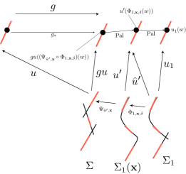
Figure 9. $I_{\hat{u}^{\prime},{\bf x}}\circ I_{{\bf x}_{0},\phi_{0};((\Sigma^{\prime},\vec{z}^{\,\prime}),u^{\prime})}$

Lemma 7.55.

We fix $e$ and regard (7.47) as a map

$$U^{\prime}(\epsilon)\times\mathcal{V}_{(1)}(\epsilon)\to L^{2}_{m+1}(\Sigma_{1}(\delta);u_{1}^{*}TX\otimes\Lambda^{01}).$$

Then it is a smooth map between Hilbert spaces.

Proof.

Note $e^{i}$ and $u$ are fixed smooth maps. Moreover

$$(\hat{u}^{\prime},{\bf x})\mapsto\Psi_{\hat{u}^{\prime},{\bf x}},\qquad(\hat{u}^{\prime},{\bf x})\mapsto\Phi_{1,{\bf x},\delta}$$

are smooth families of smooth maps. Note even though $\hat{u}^{\prime}$ is only of $L^{2}_{m+1}$ class and is not smooth, the family $\Psi_{\hat{u}^{\prime},{\bf x}}$ is a smooth family of smooth maps. In fact $\hat{u}^{\prime}$ are involved here only through $g(\hat{u}^{\prime},{\bf x})$ and $\varphi(\hat{u}^{\prime},{\bf x})$. By Lemma 7.46 both $g(\hat{u}^{\prime},{\bf x})$ and $\varphi(\hat{u}^{\prime},{\bf x})$ are smooth with respect to $\hat{u}^{\prime}\in L^{2}_{m+1}$. $\Phi_{1,{\bf x},\delta}$ is independent of $\hat{u}^{\prime}$ and depend smoothly on ${\bf x}$.

Therefore

$$(\hat{u}^{\prime},{\bf x})\mapsto e^{i}\circ\Psi_{\hat{u}^{\prime},{\bf x}}\circ\Phi_{1,{\bf x},\delta},\quad(\hat{u}^{\prime},{\bf x})\mapsto u\circ\Psi_{\hat{u}^{\prime},{\bf x}}\circ\Phi_{1,{\bf x},\delta}$$

are smooth maps.

The lemma then follows immediately from the smoothness of $g(\cdot,\cdot)$, ${\rm Pal}^{i}_{j}(\cdot)$, $G(\cdot)_{j}^{i}$, $\mathfrak{f}(\cdot,\cdot,\cdot)$. (We use also the fact that $v\mapsto F\circ v$ is a smooth map between $L^{2}_{m+1}$ spaces if $F$ is a smooth map and $m$ is sufficiently large.) ∎

Now we are in the position to complete the proof of Proposition 7.14. We take a partition of unity $\chi_{\sigma}$ subordinate to the covering $W_{\sigma}$. Let $e_{1},\dots,e_{d}$ be a basis of $E((\Sigma,\vec{z}),u)$. We put

(7.48) $$e_{i}(\hat{u}^{\prime},{\bf x})=I_{\hat{u}^{\prime},{\bf x}}(I_{{\bf x}_{0},\phi_{0};((\Sigma^{\prime},\vec{z}^{\,\prime}),u^{\prime})}(g(\hat{u}^{\prime},{\bf x})_{*}(e_{i})))$$

as in the right hand side of (7.47). By definition $(e_{i}(\hat{u}^{\prime},{\bf x}))_{i=1}^{d}$ is a basis of $E(\hat{u}^{\prime},{\bf x})$.

On the other hand since

$$e_{i}(\hat{u}^{\prime},{\bf x})=\sum_{\sigma}I_{\hat{u}^{\prime},{\bf x}}(I_{{\bf x}_{0},\phi_{0};((\Sigma^{\prime},\vec{z}^{\,\prime}),u^{\prime})}(g(\hat{u}^{\prime},{\bf x})_{*}(\chi_{\sigma}e_{i})))$$

Lemma 7.55 implies that $(\hat{u}^{\prime},{\bf x})\mapsto e_{i}(\hat{u}^{\prime},{\bf x})$ is smooth. The proof of Proposition 7.14 is complete. ∎

7.5. Independence of the local smooth structure of the choices

In this subsection we prove Proposition 7.36. Let $\mathfrak{p}_{i}=((\Sigma_{i},\vec{z}_{i}),u_{i})\in U(((\Sigma,\vec{z}),u);\epsilon_{2})$ for $i=1,2$ and we take strong stabilization data $({\mathfrak{W}}^{(i)},\vec{\mathcal{N}}_{i})$ (Definition 7.5) at $\mathfrak{p}_{i}$ for $i=1,2$.

We obtained a map

$$\mathscr{I}_{i,\epsilon_{(i)}}:V(\mathfrak{p}_{i};\epsilon_{(i)},({\mathfrak{W}}^{(i)},\vec{\mathcal{N}}_{i}))\to U(((\Sigma,\vec{z}),u);\epsilon_{2})$$

which is $\mathcal{G}_{i}$-equivariant for sufficiently small $\epsilon_{2}$. (Note $\mathcal{G}_{i}$ is the group of automorphisms of $\mathfrak{p}_{i}=((\Sigma_{i},\vec{z}_{i}),u_{i})$ and is a finite group. $\epsilon_{(1)}=\epsilon$, $\epsilon_{(2)}=\epsilon^{\prime}$.)

In fact

(7.49) $$\mathscr{I}_{i,\epsilon_{(i)}}({\bf v},{\bf x})=[(\Sigma_{i}({\bf x}),\vec{z}_{i}({\bf x})),u^{i}_{{\bf v},{\bf x}}].$$

See Proposition 7.16 and Definition 7.22. Note $u^{i}_{{\bf v},{\bf x}}$ is $u_{{\bf v},{\bf x}}$ in Proposition 7.16. Since this map depends on $\mathfrak{p}_{i}$ and ${\mathfrak{W}}^{(i)}$ we put superscript $i$ and write $u^{i}_{{\bf v},{\bf x}}$.

Suppose $\mathfrak{p}_{2}=((\Sigma_{2},\vec{z}_{2}),u_{2})$ is $\epsilon$-close to $\mathfrak{p}_{1}=((\Sigma_{1},\vec{z}_{1}),u_{1})$ for some $\epsilon$ depending on $\mathfrak{p}_{1}$. Then $\mathcal{G}_{2}\subset\mathcal{G}_{1}$.

To prove Proposition 7.36 it suffices to find a $\mathcal{G}_{2}$-equivariant $C^{n}$ open embedding

$$\mathscr{J}_{12;\epsilon,\epsilon^{\prime}}:V(\mathfrak{p}_{2};\epsilon^{\prime},({\mathfrak{W}}^{(2)},\vec{\mathcal{N}}_{2}))\to V(\mathfrak{p}_{1};\epsilon,({\mathfrak{W}}^{(1)},\vec{\mathcal{N}}_{1}))$$

such that

(7.50) $$\mathscr{I}_{1,\epsilon}\circ\mathscr{J}_{12;\epsilon,\epsilon^{\prime}}=\mathscr{I}_{2,\epsilon^{\prime}},$$

for sufficiently small $\epsilon^{\prime}$.

Existence of such a map $\mathscr{J}_{12;\epsilon,\epsilon^{\prime}}$ (set theoretically) is a consequence of Proposition 7.16. We will prove that it is a $C^{n}$ map using the exponential decay estimate, Proposition 7.17. We will prove Lemma 7.27 at the same time. The detail follows.

Our proof is divided into various cases. In the first four cases we assume $\mathfrak{p}_{1}=\mathfrak{p}_{2}$.

(Case 1) We assume $\mathfrak{p}_{1}=\mathfrak{p}_{2}=((\Sigma_{1},\vec{z}_{1}),u_{1})$. We also require $({\mathfrak{W}}^{(1)},\vec{\mathcal{N}}_{1})\subseteq({\mathfrak{W}}^{(2)},\vec{\mathcal{N}}_{2})$ in the following sense.

1. Let $\vec{w}_{1}^{\,(i)}=(w_{1,1}^{(i)},\dots,w_{1,k_{i}}^{(i)})$. We assume $k_{1}\leq k_{2}$ and $w_{1,j}^{(1)}=w_{1,j}^{(2)}$ for $j=1,\dots,k_{1}$.

2. We require $\mathcal{N}_{j}^{(1)}=\mathcal{N}_{j}^{(2)}$ for $j=1,\dots,k_{1}$.

We consider an open neighborhood $\mathcal{V}_{(i)}\subset\mathcal{M}_{g,\ell+k_{i}}$ of $(\Sigma_{1},\vec{z}_{1}\cup\vec{w}_{1}^{\,(i)})$ and the universal family of deformation $\pi_{(i)}:\mathcal{C}_{(i)}\to\mathcal{V}_{(i)}$ on it. It comes with sections $\mathfrak{t}^{(i)}_{j}:\mathcal{V}_{(i)}\to\mathcal{C}_{(i)}$, $j=1,\dots,\ell+k_{i}$, which assigns the $j$-th marked point.

Lemma 7.56.

There exists holomorphic maps $\tilde{\psi}:\mathcal{C}_{(2)}\to\mathcal{C}_{(1)}$ and $\psi:\mathcal{V}_{(2)}\to\mathcal{V}_{(1)}$ such that the following holds.

1. The next diagram commutes and is cartesian.

   (7.51) $$\begin{CD}\mathcal{C}_{(2)}@ >{\tilde{\psi}}>>\mathcal{C}_{(1)},\\ @ VV{\pi_{(2)}}V@ VV{\pi_{(1)}}V\\ \mathcal{V}_{(2)}@ >{\psi}>>\mathcal{V}_{(1)},\end{CD}$$

2. The next diagram commutes for $j=1,\dots,\ell+k_{1}$.

   (7.52) $$\begin{CD}\mathcal{C}_{(2)}@ >{\tilde{\psi}}>>\mathcal{C}_{(1)},\\ @ AA{\mathfrak{t}_{j}^{(2)}}A@ AA{\mathfrak{t}_{j}^{(1)}}A\\ \mathcal{V}_{(2)}@ >{\psi}>>\mathcal{V}_{(1)},\end{CD}$$

3. $\tilde{\psi}$ and $\psi$ are $\mathcal{G}_{2}$ equivariant.

4. $\psi$ is a submersion and the complex dimension of its fibers are $k_{2}-k_{1}$.

Proof.

By forgetting $k_{1}+1,\dots,k_{2}$-th marked points $\pi_{(2)}:\mathcal{C}_{(2)}\to\mathcal{V}_{(2)}$ becomes a deformation of $(\Sigma_{1},\vec{z}_{1}\cup\vec{w}_{1}^{\,(1)})$. Therefore we obtain desired maps $\tilde{\psi}$ and $\psi$ by the universality of $\pi_{(1)}:\mathcal{C}_{(1)}\to\mathcal{V}_{(1)}$ (together with $\mathfrak{t}_{j}^{(1)}$’s.) ∎

The proof of Lemma 7.27 in Case 1.

For the proof of Lemma 7.27 we consider the situation when we are given stabilization and trivialization data ${\mathfrak{W}}^{(i)}$. We assume Item (1-1) only. ((1-2) does not make sense.) We assume $[(\Sigma_{2},\vec{z}_{2}),u_{2}]=[(\Sigma_{1},\vec{z}_{1}),u_{1}]$ and

$$[(\Sigma(c),\vec{z}_{c}),u_{c}]\in\mathcal{U}(\epsilon(c);(\Sigma_{2},\vec{z}_{2}),u_{2},{\mathfrak{W}}^{(2)})$$

with $\lim_{c\to\infty}\epsilon(c)\to 0$. It suffices to show $[(\Sigma(c),\vec{z}_{c}),u_{c}]\in\mathcal{U}(\epsilon;(\Sigma_{1},\vec{z}_{1}),u_{1},{\mathfrak{W}}^{(1)})$ for sufficiently large $c$. By assumption there exists ${\bf x}_{c}\in\mathcal{V}_{(2)}$ converging to the origin $o$, the $k_{2}$ extra marked points $\vec{w}_{c}\subset\Sigma(c)$ and isomorphisms

$$\phi_{c}:(\Sigma^{(2)}({\bf x}_{c}),\vec{z}^{\,(2)}({\bf x}_{c})\cup\vec{w}^{\,(2)}({\bf x}_{c}))\to(\Sigma(c),\vec{z}_{c}\cup\vec{w}_{c}).$$

(Here $(\Sigma^{(2)}({\bf x}_{c}),\vec{z}^{\,(2)}({\bf x}_{c})\cup\vec{w}^{\,(2)}({\bf x}_{c}))$ is a marked stable curve of genus $g$ and $\ell+k_{2}$ marked points representing ${\bf x}_{c}$. We identify $\Sigma(c)$ with the fiber $\pi_{(2)}^{-1}({\bf x}_{c})$.) Moverover there exists $\delta_{c}<\epsilon(c)$ such that:

1. The $C^{2}$ norm of the difference between $u_{c}\circ\phi_{c}\circ\Phi_{2,{\bf x}_{c},\delta_{c}}$ and $u_{2}$ is smaller than $o(c)$.

2. The map $u_{c}\circ\phi_{c}$ has diameter $<o(c)$ on $\Sigma^{(2)}({\bf x}_{c})\setminus{\rm Im}(\Phi_{2,{\bf x}_{c},\delta_{c}})$.

We put ${\bf x}^{\prime}_{c}=\psi({\bf x}_{c})$. We define $\vec{w}^{\,\prime}_{c}$ by forgetting the last $k_{2}-k_{1}$ marked points of $\vec{w}_{c}$. We have an isomorphism

$$\phi^{\prime}_{c}:(\Sigma^{(1)}({\bf x}^{\prime}_{c}),\vec{z}^{\,(1)}({\bf x}^{\prime}_{c})\cup\vec{w}^{\,(1)}({\bf x}^{\prime}_{c}))\to(\Sigma(c),\vec{z}_{c}\cup\vec{w}^{\,\prime}_{c}).$$

We have

$$\phi^{\prime}_{c}\circ\tilde{\psi}|_{\Sigma^{(2)}({\bf x}_{c})}=\phi_{c}.$$

Note $\Phi_{2,{\bf x}_{c},\delta_{c}}$ and $\Phi_{1,{\bf x}^{\prime}_{c},\delta_{c}}$ both converge to the identity map as maps $\Sigma_{i}(\delta_{c})\to\mathcal{C}_{(i)}$, in $C^{2}$ topology. Therefore the $C^{2}$ difference between

$$\tilde{\psi}|_{\Sigma^{(2)}({\bf x}_{c})}\circ\Phi_{2,{\bf x}_{c},\delta_{c}}\quad\text{and}\quad\Phi_{1,{\bf x}^{\prime}_{c},\delta_{c}}$$

goes to $0$ as $c\to\infty$. Therefore the $C^{2}$ difference between

$$u_{c}\circ\phi_{c}\circ\Phi_{2,{\bf x}_{c},\delta_{c}}\quad\text{and}\quad u_{c}\circ\phi^{\prime}_{c}\circ\Phi_{1,{\bf x}^{\prime}_{c},\delta_{c}}$$

goes to $0$ as $c\to\infty$. Therefore by (1) the $C^{2}$ difference between

$$u_{1}\quad\text{and}\quad u_{c}\circ\phi^{\prime}_{c}\circ\Phi_{1,{\bf x}^{\prime}_{c},\delta_{c}}$$

goes to $0$ as $c\to\infty$. (Note $u_{1}=u_{2}$.)

Sublemma 7.57.

The map $u_{c}\circ\phi^{\prime}_{c}$ has diameter $<o(c)$ on $\Sigma^{(1)}({\bf x}^{\prime}_{c})\setminus{\rm Im}(\Phi_{1,{\bf x}^{\prime}_{c},\delta_{c}})$.

Proof.

There exists $\delta^{+}_{c}\to 0$ such that $\delta^{+}_{c}>\delta_{c}$ and

$${\rm Im}(\Phi_{1,{\bf x}^{\prime}_{c},\delta_{c}})\supset\tilde{\psi}({\rm Im}(\Phi_{2,{\bf x}_{c},\delta^{+}_{c}})).$$

Let $W$ be a connected component of $\Sigma^{(1)}({\bf x}_{c^{\prime}})\setminus{\rm Im}(\Phi_{1,{\bf x}^{\prime}_{c},\delta_{c}})$. There exists a connected component $W_{+}$ of $\Sigma^{(1)}({\bf x}_{c^{\prime}})\setminus\tilde{\psi}({\rm Im}(\Phi_{2,{\bf x}_{c},\delta^{+}_{c}}))$ which contains it. It suffices to show

(7.53) $$\lim_{c\to\infty}{\rm Diam}(u_{c}\circ\phi^{\prime}_{c})(W_{+})=0.$$

Note

$$\partial W_{+}\ =\tilde{\psi}(\partial({\rm Im}(\Phi_{2,{\bf x}_{c},\delta^{+}_{c}}))=(\tilde{\psi}\circ\Phi_{2,{\bf x}_{c},\delta^{+}_{c}})(\partial\Sigma_{1}(\delta_{c}^{+})).$$

On $\partial\Sigma_{1}(\delta_{c}^{+})$, the map $u_{c}\circ\phi^{\prime}_{c}\circ\tilde{\psi}\circ\Phi_{2,{\bf x}_{c},\delta^{+}_{c}}=u_{c}\circ\phi_{c}\circ\Phi_{2,{\bf x}_{c},\delta^{+}_{c}}$ is $C^{2}$ close to $u_{1}$. Since $\delta_{c}^{+}\to 0$,

$$\lim_{c\to\infty}{\rm Diam}(u_{c}\circ\phi_{c}\circ\Phi_{2,{\bf x}_{c},\delta^{+}_{c}})(\partial\Sigma_{1}(\delta_{c}^{+}))=0.$$

Therefore

$$\lim_{c\to\infty}{\rm Diam}(u_{c}\circ\phi^{\prime}_{c})(\partial W_{+})=0.$$

Since $u_{c}\circ\phi^{\prime}_{c}$ is holomorphic on $W_{+}$ (this is because it satisfies the equation (6.12) in Definition 6.14 and the supports of the elements of the obstruction spaces are away from $W_{+}$), the formula (7.53) follows. ∎

Therefore $[(\Sigma(c),\vec{z}_{c}),u_{c}]\in\mathcal{U}(\epsilon;(\Sigma_{1},\vec{z}_{1}),u_{1},{\mathfrak{W}}^{(1)})$ for sufficiently large $c$. ∎

Proof of Proposition 7.36 in Case 1.

For ${\bf x}\in\mathcal{V}_{(i)}$ we denote by $(\Sigma_{1}^{(i)}({\bf x}),\vec{z}_{1}^{\,(i)}({\bf x})\cup\vec{w}_{1}^{\,(i)}({\bf x}))$ the fiber $\pi_{(i)}^{-1}({\bf x})$ together with marked points.

For ${\bf x}\in\mathcal{V}_{(2)}$, (7.8) defines an open embedding

(7.54) $$\Phi^{(2)}_{1,{\bf x},\delta^{\prime}}:\Sigma_{1}(\delta^{\prime})\to\Sigma_{1}^{(2)}({\bf x})$$

which is canonically determined by the data ${\mathfrak{W}}^{(2)}$. The restriction of $\tilde{\psi}$ to the fiber $\Sigma_{1}^{(2)}({\bf x})$ defines a map (isomorphism)

(7.55) $$\tilde{\psi}_{\bf x}:\Sigma_{1}^{(2)}({\bf x})\to\Sigma_{1}^{(1)}(\psi({\bf x})).$$

If $\delta^{\prime}$ is sufficiently small compared to $\delta$, we compose the maps the inverse of (7.54), (7.55) and $\Phi^{(1)}_{1,\psi({\bf x}),\delta}$ (which is defined also by (7.8)) to obtain

(7.56) $$\Psi_{{\bf x}}=(\Phi^{(2)}_{1,{\bf x},\delta^{\prime}})^{-1}\circ\tilde{\psi}_{\bf x}^{-1}\circ\Phi^{(1)}_{1,\psi({\bf x}),\delta}:\Sigma_{1}(\delta)\to\Sigma_{1}(\delta^{\prime}).$$

The next lemma is obvious.

Lemma 7.58.

The map $\hat{\Psi}:\mathcal{V}_{(2)}\to C^{\infty}(\Sigma_{1}(\delta),\Sigma_{1}(\delta^{\prime}))$ which assigns $\Psi_{{\bf x}}$ to ${\bf x}$ is a $C^{\infty}$ map.

We next recall the following standard fact.

Lemma 7.59.

The map

$${\rm comp}:L^{2}_{m+n+1}(\Sigma_{1}(\delta^{\prime}),X)\times C^{\infty}(\Sigma_{1}(\delta),\Sigma_{1}(\delta^{\prime}))\to L^{2}_{m+1}(\Sigma_{1}(\delta),X)$$

defined by

$${\rm comp}(F,\phi)=F\circ\phi$$

is a $C^{n}$ map in a neighborhood of $(F_{0},\phi_{0})$ if $m>10$ and $\phi_{0}$ is an open embedding.

We take sufficiently large $m$ and put $m_{1}=m+n$, $m_{2}=m+2n$. Note $\mathcal{V}_{\rm map}(\epsilon)$ is the $\epsilon$ neighborhood of $0$ in ${\rm Ker}^{+}D_{u_{1}}\overline{\partial}$. So this space is the same for ${\mathfrak{W}}^{(1)}$ and ${\mathfrak{W}}^{(2)}$.

We next define a map

$$\mathcal{R}_{(i)}:\mathcal{V}_{\rm map}(\epsilon)\times\mathcal{V}_{(i)}(\epsilon)\to L^{2}_{m_{i}+1-n}(\Sigma_{1}(\delta^{(i)}),X)\times\mathcal{V}_{(i)}(\epsilon).$$

Here $\delta^{(1)}=\delta$, $\delta^{(2)}=\delta^{\prime}$ and $\mathcal{V}_{(i)}(\epsilon)$ is defined as follows. Recall for ${\bf x}\in\mathcal{V}_{(1)}(\epsilon)$ and ${\bf v}\in\mathcal{V}_{\rm map}(\epsilon)$ the map $u^{i}_{{\bf v},{\bf x}}$ is defined. (See Proposition 7.16.) $\mathcal{V}_{(1)}(\epsilon)$ is an open neighborhood of $(\Sigma_{1},\vec{z}_{1}\cup\vec{w}_{i})$ in $\mathcal{M}_{g,\ell+k_{i}}$. Note $\mathcal{V}_{(1)}(\epsilon)$ are actually ${\mathfrak{W}}^{(i)}$ and $i$ dependent. We define:

(7.57) $$\mathcal{R}_{(i)}({\bf v},{\bf x})=(u^{i}_{{\bf v},{\bf x}}\circ\Phi^{(i)}_{1,{\bf x},\delta^{(i)}},{\bf x})$$

Lemma 7.60.

We put the smooth structure on $\mathcal{V}_{(i)}(\epsilon)$ as in Definition 7.19. Then $\mathcal{R}_{(i)}$ is a $C^{n}$ embedding for sufficiently small $\epsilon$.

Proof.

The fact that $\mathcal{R}_{(i)}$ is a $C^{n}$ map is a consequence of Proposition 7.17. The derivative of the first factor of $\mathcal{R}_{(i)}$ at $(0,o_{i})$ restricts to an embedding

$$T_{0}V_{\rm map}(\epsilon)\to L^{2}_{m_{i}+1-n}(\Sigma_{1}(\delta^{(i)}),u_{i}^{*}TX).$$

Here $\mathcal{R}_{(i)}(0,o_{i})=(u_{i},o_{i})$ and $o_{i}=[\Sigma_{1},\vec{z}_{1}\cup\vec{w}_{i}]$. The injectivity of this map is a consequence of unique continuation. Note $\mathcal{V}_{(i)}(\epsilon)$ factor of $\mathcal{R}_{(i)}$ is $({\bf v},{\bf x})\mapsto\bf x$. Therefore the derivative of $\mathcal{R}_{(i)}$ is injective at $(0,o_{i})$. The lemma now follows from the inverse function theorem. ∎

We define a map

$$\Phi:L^{2}_{m_{2}+1-n}(\Sigma_{1}(\delta^{(2)}),X)\times\mathcal{V}_{(2)}(\epsilon)\to L^{2}_{m_{1}+1-n}(\Sigma_{1}(\delta^{(1)}),X)\times\mathcal{V}_{(1)}(\epsilon)$$

by

(7.58) $$\Phi(F,{\bf x})=(F\circ\Psi_{{\bf x}},\psi({\bf x}))$$

Lemma 7.61.

For small $\epsilon$ there exist positive numbers $\epsilon^{\prime}$,$\delta^{\prime}$ and a $C^{n}$-map

$$\tilde{\mathscr{J}}:\mathcal{V}_{\rm map}(\epsilon^{\prime})\times\mathcal{V}_{(2)}(\epsilon^{\prime})\to\mathcal{V}_{\rm map}(\epsilon)\times\mathcal{V}_{(1)}(\epsilon)$$

such that the next diagram commutes.

(7.59) $$\begin{CD}\mathcal{V}_{\rm map}(\epsilon^{\prime})\times\mathcal{V}_{(2)}(\epsilon^{\prime})@ >{\mathcal{R}_{(2)}}>>L^{2}_{m_{2}+1-n}(\Sigma_{1}(\delta^{\prime}),X)\times\mathcal{V}_{(2)}(\epsilon^{\prime})\\ @ VV{\tilde{\mathscr{J}}}V@ VV{\Phi}V\\ \mathcal{V}_{\rm map}(\epsilon)\times\mathcal{V}_{(1)}(\epsilon)@ >{\mathcal{R}_{(1)}}>>L^{2}_{m_{1}+1-n}(\Sigma_{1}(\delta),X)\times\mathcal{V}_{(1)}(\epsilon).\end{CD}$$

Proof.

The existence of a map $\tilde{\mathscr{J}}$ such that the diagram (7.59) commutes is a consequence of Proposition 7.16 as follows.

Let ${\bf v}\in\mathcal{V}_{\rm map}(\epsilon)$, ${\bf x}\in\mathcal{V}_{(i)}(\epsilon)$. Then

$$\Phi(\mathcal{R}_{(2)}({\bf v},{\bf x}))=(u^{2}_{{\bf v},{\bf x}}\circ\Phi^{(2)}_{1,{\bf x},\delta^{\prime}}\circ\Psi_{\bf x},\psi({\bf x}))$$

Note $\Psi_{\bf x}=(\Phi^{(2)}_{1,{\bf x},\delta^{\prime}})^{-1}\circ\tilde{\psi}_{\bf x}^{-1}\circ\Phi^{(1)}_{1,\psi({\bf x}),\delta}$.

We put

$$u^{\prime}=u^{2}_{{\bf v},{\bf x}}\circ\tilde{\psi}_{\bf x}^{-1}:\Sigma_{1}(\psi({\bf x}))\to X.$$

Since $\tilde{\psi}_{\bf x}:(\Sigma_{2}({\bf x}),\vec{z}_{2}({\bf x}))\cong(\Sigma_{1}(\psi({\bf x})),\vec{z}_{1}(\psi({\bf x}))$ is a bi-holomorphic map

$$\overline{\partial}u^{2}_{{\bf v},{\bf x}}\in E((\Sigma_{2}({\bf x}),\vec{z}_{2}({\bf x})),u^{2}_{{\bf v},{\bf x}})$$

implies

(7.60) $$\overline{\partial}u^{\prime}\in E((\Sigma_{1}(\psi({\bf x})),\vec{z}_{1}(\psi({\bf x})),u^{\prime}).$$

Moreover the $C^{2}$ distance between

$$u^{\prime}\circ\Phi^{(1)}_{1,\psi({\bf x}),\delta}\qquad\text{and}\qquad u^{2}_{{\bf v},{\bf x}}\circ\Phi^{(2)}_{1,{\bf x},\delta}$$

goes to $0$ as $\epsilon\to 0$ by Lemma 7.16 (4). By assumption the $C^{2}$ distance between

$$u^{2}_{{\bf v},{\bf x}}\circ\Phi^{(2)}_{1,{\bf x},\delta}\qquad\text{and}\qquad u_{2}=u_{1}$$

is smaller than $\epsilon^{\prime}$. Therefore the $C^{2}$ distance between

$$u^{\prime}\circ\Phi^{(1)}_{1,\psi({\bf x}),\delta}\qquad\text{and}\qquad u_{2}=u_{1}$$

is small. We can show that the map $u^{\prime}$ has diameter $<\epsilon$ on the complement of the image of $\Phi^{(1)}_{1,\psi({\bf x}),\delta}$ if $\epsilon^{\prime}$ is sufficiently small, using the fact that $\mathfrak{p}_{2}$ is $\epsilon$ close to $\mathfrak{p}_{1}$ with respect to ${\mathfrak{W}}^{(1)}$. (We use Lemma 7.9 here.) Moreover $d(o,\psi({\bf x}))$ goes to $0$ as $d(o,{\bf x})$ goes to zero.

Therefore by Proposition 7.16 (2) there exists ${\bf v}^{\prime}$ such that

(7.61) $$u^{\prime}=u^{1}_{{\bf v}^{\prime},\psi({\bf x})}.$$

Then

(7.62) $$u^{1}_{{\bf v}^{\prime},\psi({\bf x})}\circ\Phi^{(1)}_{1,\psi({\bf x}),\delta}=u^{2}_{{\bf v},{\bf x}}\circ\tilde{\psi}_{\bf x}^{-1}\circ\Phi^{(1)}_{1,\psi({\bf x}),\delta}=u^{2}_{{\bf v},{\bf x}}\circ\Phi^{(2)}_{1,{\bf x},\delta}\circ\Psi_{\bf x}.$$

By putting

$$\tilde{\mathscr{J}}({\bf v},{\bf x})=({\bf v}^{\prime},\psi({\bf x}))$$

Diagram 7.59 commutes.

Lemmata 7.58 and 7.59 then imply that $\Phi$ is a $C^{n}$ map. Lemma 7.60 implies that $\mathcal{R}_{(i)}$ are $C^{n}$ embedding. Therefore the commutativity of Diagram 7.59 implies that $\tilde{\mathscr{J}}$ is a $C^{n}$ map. ∎

By definition $V(\mathfrak{p}_{i};\epsilon_{(i)},({\mathfrak{W}}^{(i)},\vec{\mathcal{N}}_{i}))$ (See Definition 7.22) is a submanifold of $\mathcal{V}_{\rm map}(\epsilon_{(i)})\times\mathcal{V}_{(i)}(\epsilon_{(i)})$. (Here $\epsilon_{(1)}=\epsilon$, $\epsilon_{(2)}=\epsilon^{\prime}$.)

Lemma 7.62.

There exists a map $\mathscr{J}_{12;\epsilon,\epsilon^{\prime}}:V(\mathfrak{p}_{2};\epsilon^{\prime},({\mathfrak{W}}^{(2)},\vec{\mathcal{N}}_{2}))\to V(\mathfrak{p}_{1};\epsilon,({\mathfrak{W}}^{(1)},\vec{\mathcal{N}}_{1}))$ such that the next diagram commutes.

(7.63) $$\begin{CD}V(\mathfrak{p}_{2};\epsilon^{\prime},({\mathfrak{W}}^{(2)},\vec{\mathcal{N}}_{2}))@ >{}>>\mathcal{V}_{\rm map}(\epsilon^{\prime})\times\mathcal{V}_{(2)}(\epsilon^{\prime})\\ @ V{\mathscr{J}_{12;\epsilon,\epsilon^{\prime}}}VV@ V{\tilde{\mathscr{J}}}VV\\ V(\mathfrak{p}_{1};\epsilon,({\mathfrak{W}}^{(1)},\vec{\mathcal{N}}_{1}))@ >{}>>\mathcal{V}_{\rm map}(\epsilon)\times\mathcal{V}_{(1)}(\epsilon),\end{CD}$$

where horizontal arrows are canonical inclusions. Moreover $\mathscr{J}_{12;\epsilon,\epsilon^{\prime}}$ is of $C^{n}$ class.

Proof.

Let $({\bf v},{\bf x})\in V(\mathfrak{p}_{2};\epsilon^{\prime},({\mathfrak{W}}^{(2)},\vec{\mathcal{N}}_{2}))$. By Definition 7.22 we have

$$u^{2}_{{\bf v},{\bf x}}(w_{2,j}({\bf x}))\in\mathcal{N}_{j}^{(2)},$$

for $j=1,\dots,k_{2}$. We remark $\mathcal{N}_{j}^{(1)}=\mathcal{N}_{j}^{(2)}$ for $j=1,\dots,k_{1}$ by our choice. Let $({\bf v}^{\prime},{\psi}({\bf x}))=\tilde{\mathscr{J}}({\bf v},{\bf x})$. Then by the commutativity of Diagram (7.59) and (7.61) (7.62), we have

$$u^{1}_{{\bf v}^{\prime},{\psi}({\bf x})}=u^{2}_{{\bf v},{\bf x}}\circ\tilde{\psi}_{\bf x}^{-1}.$$

By the commutativity of Diagram (7.51)

$$u^{1}_{{\bf v}^{\prime},{\psi}({\bf x})}(w_{1,j}({\bf x}))=u^{1}_{{\bf v}^{\prime},{\psi}({\bf x})}(\tilde{\psi}_{\bf x}(w_{2,j}({\bf x}))=u^{2}_{{\bf v},{\bf x}}(w_{2,j}({\bf x}))\in\mathcal{N}_{j}^{(2)},$$

for $j=1,\dots,k_{1}$. Therefore by Definition 7.22

$$\tilde{\mathscr{J}}({\bf v},{\bf x})=({\bf v}^{\prime},{\psi}({\bf x}))\in V(\mathfrak{p}_{1};\epsilon,({\mathfrak{W}}^{(1)},\vec{\mathcal{N}}_{1})).$$

We thus find the map $\mathscr{J}_{12;\epsilon,\epsilon^{\prime}}$ such that Diagram (7.63) commutes. Since the horizontal arrows are $C^{n}$ embeddings and right vertical arrow is a $C^{n}$ map, the map $\mathscr{J}_{12;\epsilon,\epsilon^{\prime}}$ is of $C^{n}$ class as required. ∎

Commutativity of Diagrams (7.59) and (7.63) implies that $\mathscr{J}_{12;\epsilon,\epsilon^{\prime}}$ is $\mathcal{G}_{1}$ equivariant and (7.50) commutes.

We finally show that $\mathscr{J}_{12;\epsilon,\epsilon^{\prime}}$ is an open embedding. We consider two sub-cases.

(Case 1-1) $k_{1}=k_{2}$.

In this case $\vec{w}_{1}=\vec{w}_{2}$, $\vec{\mathcal{N}}_{1}=\vec{\mathcal{N}}_{2}$. The difference of ${\mathfrak{W}}^{(1)}$ and ${\mathfrak{W}}^{(2)}$ is the trivialization data and the analytic families of coordinates.

Lemma 7.63.

In Case 1-1, the map $\tilde{\mathscr{J}}$ in Diagram (7.59) is an open embedding.

Proof.

Since $\vec{w}_{1}=\vec{w}_{2}$ we can exchange the role of ${\mathfrak{W}}^{(1)}$ and ${\mathfrak{W}}^{(2)}$. Then by definition $\Phi_{{\bf x}}$ will become $\Phi_{\psi({\bf x})}^{-1}$. Thus $\mathscr{J}_{21;\epsilon^{\prime},\epsilon}$ obtained by exchanging the role of ${\mathfrak{W}}^{(1)}$ and ${\mathfrak{W}}^{(2)}$ is the inverse of $\mathscr{J}_{12;\epsilon,\epsilon^{\prime}}$. ∎

Since $\mathcal{N}_{j}^{(1)}=\mathcal{N}_{j}^{(2)}$ and $\#\vec{w}_{1}=\#\vec{w}_{2}$, the equations to cut down $V(\mathfrak{p}_{i};\epsilon,({\mathfrak{W}}^{(i)},\vec{N}_{i}))$ from $\mathcal{V}_{\rm map}(\epsilon)\times\mathcal{V}_{(i)}(\epsilon)$ coincide each other for $i=1,2$. Therefore $\mathscr{J}_{12;\epsilon,\epsilon^{\prime}}$ is an open embedding in Case 1-1. We thus proved Proposition 7.36 in Case 1-1. ∎

(Case 1-2) We show that, in case $\mathfrak{p}_{1}=\mathfrak{p}_{2}$ and Case 1, we can change the trivialization data and analytic families of coordinates of ${\mathfrak{W}}^{(2)}$ to obtain ${\mathfrak{W}}^{(3)}$ so that $\mathscr{J}_{13;\epsilon,\epsilon^{\prime\prime}}$ is an open embedding.

We consider irreducible component $\Sigma_{1,a}$ of $\Sigma_{1}$ and corresponding irreducible component $\Sigma_{3,a}$ of $\Sigma_{3}=\Sigma_{1}$. Forgetful map of the marked points determines the following commutative diagram.

(7.64) $$\begin{CD}\mathcal{C}_{g_{a},\ell_{a}+k_{2,a}}@ >{\tilde{\psi}}>>\mathcal{C}_{g_{a},\ell_{a}+k_{1,a}},\\ @ VV{\pi}V@ VV{\pi}V\\ \mathcal{M}_{g_{a},\ell_{a}+k_{2,a}}@ >{\psi}>>\mathcal{M}_{g_{a},\ell_{a}+k_{1,a}},\end{CD}$$

Here $\ell_{a}+k_{1,a}$ (resp. $\ell+k_{2,a}=\ell+k_{3,a}$) is the number of marked or nodal points on $\Sigma_{1,a}$ (resp. $\Sigma_{3,a}$). (Note $k_{a}=\#(\vec{w}_{1}\cap\Sigma_{1,a})$.) The vertical arrows are projections of the universal families of deformations of $\Sigma_{i,a}$ together with marked points.

Lemma 7.64.

We may take the trivialization data of ${\mathfrak{W}}^{(3)}$ so that the next diagram commutes.

(7.65) $$\begin{CD}\mathcal{V}_{3,a}\times\Sigma_{3,a}@ >{\phi_{a}^{(3)}}>>\mathcal{C}_{g_{a},\ell_{a}+k_{2,a}}\\ @ V{\psi\times{\rm id}}VV@ V{\tilde{\psi}}VV\\ \mathcal{V}_{1,a}\times\Sigma_{1,a}@ >{\phi_{a}^{(1)}}>>\mathcal{C}_{g_{a},\ell_{a}+k_{1,a}}.\end{CD}$$

Here the maps $\phi_{a}^{(3)}$, $\phi_{a}^{(1)}$ have the properties of the maps $\phi_{a}$ in Definition 7.2 (2).

Proof.

We can define $\phi_{a}^{(3)}$ by Diagram (7.65) itself. ∎

Remark 7.65.

We remark that when we make the choice as in Lemma 7.64 the $\Sigma_{3,a}$ factor of $(\phi_{a}^{(3)})^{-1}(w_{3,j}({\bf x}))$ cannot be independent of ${\bf x}$ for $j>k_{1}$. Namely (7.5) does not hold for those marked points of $\Sigma_{3}$. This is the reason why we do not assume (7.5) for marked points of $\Sigma_{i}$ but only for nodal points.

We next choose the analytic family of coordinates $\varphi_{3,a,j}:\mathcal{V}_{3,a}\times D^{2}(2)\to\mathcal{C}_{g_{a},\ell_{a}+k_{2,a}}$ for marked points on $\Sigma_{3}$ corresponding to nodal points of $\Sigma_{3}$ as follows. Let $\varphi_{1,a,j}:\mathcal{V}_{1,a}\times D^{2}(2)\to\mathcal{C}_{g_{a},\ell_{a}+k_{1,a}}$ be the analytic family of coordinates associated to ${\mathfrak{W}}^{(1)}$ for the corresponding nodal of $\Sigma_{1}$. (Note $\Sigma_{1}=\Sigma_{3}$.) We require

(7.66) $$\tilde{\psi}(\varphi_{3,a,j}({\bf x},z))=\varphi_{1,a,j}(\psi({\bf x}),z).$$

It is obvious that there is such choice of $\varphi_{3,a,j}$. By construction, the commutativity of Diagram (7.65) and (7.66) imply the next formula.

(7.67) $$\Phi_{1,\psi({\bf x}),\delta}=\tilde{\psi}\circ\Phi_{3,{\bf x},\delta}.$$

(7.67) and (7.56) imply that the map $\Phi$ defined in (7.58) is :

(7.68) $$\Phi(F,{\bf x})=(F,\psi({\bf x})).$$

We remark that the obstruction bundle $E((\Sigma^{\prime},\vec{z}^{\,\prime}),u^{\prime})$ is independent of the extra marked points $\vec{w}^{\,\prime}$. Moreover the commutativity of Diagram (7.65) implies that the identification of the source curve with $\Sigma_{1}=\Sigma_{3}$ we use during the gluing process is independent of the $\ell+k_{1}+1$-th,…,$\ell+k_{2}$ marked points. Therefore we have the next formula:

(7.69) $$u^{1}_{{\bf v},\psi({\bf x})}\circ\Phi_{1,\psi({\bf x}),\delta}=u^{3}_{{\bf v},{\bf x}}\circ\Phi_{3,{\bf x},\delta}.$$

Formulae (7.68) and (7.69) imply

(7.70) $$\tilde{\mathscr{J}}({\bf v},{\bf x})=({\bf v},\psi({\bf x}))$$

Using (7.69), (7.70) we can easily prove that $\mathscr{J}_{13;\epsilon,\epsilon^{\prime\prime}}$ is an open embedding in the same way as Lemma 7.21. We thus proved Proposition 7.36 in Case 1-2.

Now we consider the general case of Case 1. Suppose $\mathfrak{p}_{1}$ $\mathfrak{p}_{2}$ and $({\mathfrak{W}}^{(1)},\vec{\mathcal{N}}_{1})$, $({\mathfrak{W}}^{(2)},\vec{\mathcal{N}}_{2})$ are as in Case 1. Then we can take $\mathfrak{p}_{3}$ and $({\mathfrak{W}}^{(3)},\vec{\mathcal{N}}_{3})$ such that $\mathfrak{p}_{1}$, $\mathfrak{p}_{3}$ and $({\mathfrak{W}}^{(1)},\vec{\mathcal{N}}_{1})$, $({\mathfrak{W}}^{(3)},\vec{\mathcal{N}}_{3})$ are as in Case 1-2. Moreover $\mathfrak{p}_{2}$, $\mathfrak{p}_{3}$ and $({\mathfrak{W}}^{(2)},\vec{\mathcal{N}}_{2})$, $({\mathfrak{W}}^{(3)},\vec{\mathcal{N}}_{3})$ are as in Case 1-1. (Note $\mathfrak{p}_{1}=\mathfrak{p}_{2}=\mathfrak{p}_{3}$ in this case.) Therefore we obtain required $\mathscr{J}_{12;\epsilon,\epsilon^{\prime}}$ by composing $\mathscr{J}_{13;\epsilon,\epsilon^{\prime\prime}}$ and an inverse of $\mathscr{J}_{23;\epsilon^{\prime},\epsilon^{\prime\prime}}$. The proof of Proposition 7.36 in Case 1 is complete. ∎

(Case 2) We assume $\mathfrak{p}_{1}=\mathfrak{p}_{2}=((\Sigma_{1},\vec{z}_{1}),u_{1})$. We also require $({\mathfrak{W}}^{(1)},\vec{\mathcal{N}}_{1})\supseteq({\mathfrak{W}}^{(2)},\vec{\mathcal{N}}_{2})$

The proof of this case is entirely similar to Case 1 and so is omitted.

(Case 3) We assume $\mathfrak{p}_{1}=\mathfrak{p}_{2}=((\Sigma_{1},\vec{z}_{1}),u_{1})$. We also require $\vec{w}^{\,(1)}\cap\vec{w}^{(2)}=\emptyset$.

We define $({\mathfrak{W}}^{(3)},\vec{\mathcal{N}}_{3})$ as follows. $\vec{w}^{\,(3)}=\vec{w}^{\,(1)}\cup\vec{w}^{(2)}$. $\mathcal{N}^{(3)}_{j}$ is $\mathcal{N}^{(1)}_{j^{\prime}}$ (resp. $\mathcal{N}^{(2)}_{j^{\prime}}$) if $w^{(3)}_{1,j}=w^{(1)}_{1,j^{\prime}}$ (resp. $w^{(3)}_{1,j}=w^{(2)}_{1,j^{\prime}}$). We take any choice of the trivialization data and of analytic families of coordinates.

Then the triples $\mathfrak{p}_{1},({\mathfrak{W}}^{(1)},\vec{\mathcal{N}}_{1})$, and $\mathfrak{p}_{3},({\mathfrak{W}}^{(3)},\vec{\mathcal{N}}_{3})$ (resp. $\mathfrak{p}_{2},({\mathfrak{W}}^{(2)},\vec{\mathcal{N}}_{2})$ and $\mathfrak{p}_{3},({\mathfrak{W}}^{(3)},\vec{\mathcal{N}}_{3})$) satisfy the conditions for (Case 1) or (Case 2). Therefore we obtain required $\mathscr{J}_{12;\epsilon,\epsilon^{\prime}}$ by composing $\mathscr{J}_{23;\epsilon^{\prime},\epsilon^{\prime\prime}}$ and an inverse of $\mathscr{J}_{13;\epsilon,\epsilon^{\prime\prime}}$.

We can prove Lemma 7.27 also in the same way.

(Case 4) We assume $\mathfrak{p}_{1}=\mathfrak{p}_{2}=((\Sigma_{1},\vec{z}_{1}),u_{1})$ only.

We can find $({\mathfrak{W}}^{(3)},\vec{\mathcal{N}}_{3})$ with $\mathfrak{p}_{3}=\mathfrak{p}_{1}$ such that $\vec{w}^{\,(1)}\cap\vec{w}^{(3)}=\emptyset=\vec{w}^{\,(2)}\cap\vec{w}^{(3)}$. We then apply (Case 3) twice and compose the resulting maps to obtain the required $\mathscr{J}_{12;\epsilon,\epsilon^{\prime}}$.

We can prove Lemma 7.27 also in the same way. We thus completed the case $\mathfrak{p}_{1}=\mathfrak{p}_{2}$.

(Case 5) We consider the general case where $\mathfrak{p}_{1}\neq\mathfrak{p}_{2}$.

The proof of Lemma 7.27 in Case 5.

Using (Case 4) it suffices to show the following. For given stabilization and trivialization data ${\mathfrak{W}}^{(1)}$ at $\mathfrak{p}_{1}$ we can find stabilization and trivialization data ${\mathfrak{W}}^{(2)}$ at $\mathfrak{p}_{2}$ such that Lemma 7.27 holds. We will prove this statement below.

We fixed ${\mathfrak{W}}^{(1)}$, in particular we fixed $\vec{w}_{1}$. We take the universal family of deformation of $(\Sigma_{1},\vec{z}_{1}\cup\vec{w}_{1})$ and denote it by $\pi:\mathcal{C}_{(1)}\to\mathcal{V}_{(1)}$. (It comes with sections assigning marked points.)

Since $\mathfrak{p}_{2}=[\Sigma_{2},\vec{z}_{2}]$ is $\epsilon$-close to $\mathfrak{p}_{1}$ with respect to ${\mathfrak{W}}^{(1)}$ there exists ${\bf x}_{2}$ and $\vec{w}_{2}$ such that

$$\phi:(\Sigma_{1}({\bf x}_{2}),\vec{z}_{1}({\bf x}_{2})\cup\vec{w}_{1}({\bf x}_{2}))\cong(\Sigma_{2},\vec{z}_{2}\cup\vec{w}_{2}).$$

We take this $\vec{w}_{2}$ as a part of the data consisting ${\mathfrak{W}}^{(2)}$. Let $\pi:\mathcal{C}_{(2)}\to\mathcal{V}_{(2)}$ be the universal family of deformation of $(\Sigma_{2},\vec{z}_{2}\cup\vec{w}_{2})$. Then we have an open embeddings $\psi:\mathcal{V}_{(2)}\to\mathcal{V}_{(1)}$ and $\tilde{\psi}:\mathcal{C}_{(2)}\to\mathcal{C}_{(1)}$ such that Diagrams (7.51) and (7.52) commute.

Lemma 7.66.

There exist stabilization and trivialization data ${\mathfrak{W}}^{(2)}$ so that

(7.71) $$\tilde{\psi}_{\bf x}\circ\Phi_{2,{\bf x},\delta^{\prime}}=\Phi_{1,\psi({\bf x}),\delta}\circ\Phi_{1,{\bf x}_{2},\delta}^{-1}\circ\phi^{-1}$$

holds on $\phi(\Phi_{1,{\bf x}_{2},\delta}(\Sigma_{1}(\delta)))$ if $\delta^{\prime}$ is small. Here $\tilde{\psi}_{\bf x}$ is the restriction of $\tilde{\psi}$ to $\Sigma_{2}({\bf x})$.

(7.72) $$\begin{CD}(\Sigma_{1}({\bf x}_{2})(\delta)\,\,\overset{\phi}{\hookrightarrow}\,\,\Sigma_{2}(\delta^{\prime}))@ >{\Phi_{2,{\bf x},\delta^{\prime}}}>>\Sigma_{2}({\bf x})\\ @ AA{\Phi_{1,{\bf x}_{2},\delta}}A@ VV{\tilde{\psi}_{\bf x}}V\\ \Sigma_{1}(\delta)@ >{\Phi_{1,\psi({\bf x}),\delta}}>>\Sigma_{1}(\psi({\bf x})),\end{CD}$$

Proof.

$\Sigma_{1}({\bf x}_{2})\cong\Sigma_{2}$ is obtained by deforming the complex structure of irreducible components of $\Sigma_{1}$ and gluing several irreducible components along (some of) marked points.

Note the weak stabilization data $\vec{w}_{2}$ was defined by sending weak stabilization data $\vec{w}_{1}$ of ${\mathfrak{W}}^{(1)}$ by $\Phi_{1,{\bf x}_{2},\delta}$.

We define families of coordinates at the nodes which are parts of ${\mathfrak{W}}^{(2)}$ as follows. Suppose $\Sigma_{2}({\bf x}_{0})$ has the same number of nodes as $\Sigma_{2}$. Note each node of $\Sigma_{2}({\bf x}_{0})$ corresponds to an node of $\Sigma_{1}(\psi({\bf x}_{0}))$. Therefore we pull back families of coordinates at the nodes of $\Sigma_{1}(\psi({\bf x}_{0}))$ by $\tilde{\psi}_{\bf x}$ to obtain the families of coordinates at the nodes we look for. We remark that according to the definition the families of coordinates at the nodes of $\Sigma_{1}({\bf x}_{0}^{\prime})$ is given only in case $\Sigma_{1}({\bf x}_{0}^{\prime})$ has the same number of nodes as $\Sigma_{1}$. (See Definition 7.4.) However they canonically induce one of $\Sigma_{1}({\bf x}^{\prime})$ for any ${\bf x}^{\prime}$. In fact, $\Sigma_{1}({\bf x}^{\prime})$ is obtained from some $\Sigma_{1}({\bf x}^{\prime}_{0})$ (with the same number of nodes as $\Sigma_{1}$) by performing the gluing at several nodes. The nodes of $\Sigma_{1}({\bf x}^{\prime})$ correspond to the nodes of $\Sigma_{1}({\bf x}^{\prime}_{0})$ where such gluing construction were not performed. So neighborhoods of the nodes of $\Sigma_{1}({\bf x}^{\prime})$ are canonically identified with neighborhoods of certain nodes of $\Sigma_{1}({\bf x}^{\prime}_{0})$.

We finally define local trivializations. Suppose $\Sigma_{2}({\bf x}_{0})$ has the same number of nodes as $\Sigma_{2}$. We use $\phi\circ\Phi_{1,{\bf x}_{2},\delta}\circ\Phi_{1,\psi({\bf x}_{0}),\delta}^{-1}\circ\tilde{\psi}_{{\bf x}_{0}}$ to define a diffeomorphism

$$\phi\circ\Phi_{1,{\bf x}_{2},\delta}\circ\Phi_{1,\psi({\bf x}_{0}),\delta}^{-1}\circ\tilde{\psi}_{{\bf x}_{0}}:\tilde{\psi}^{-1}_{{\bf x}_{0}}(\Phi_{1,\psi({\bf x}_{0}),\delta}(\Sigma_{1}(\delta)))\to\Sigma_{1}(\delta)\to\Sigma_{1}({\bf x}_{2})\to\Sigma_{2}.$$

Here $\tilde{\psi}^{-1}_{{\bf x}_{0}}(\Phi_{1,\psi({\bf x}_{0}),\delta}(\Sigma_{1}(\delta)))\subset\Sigma_{2}({\bf x}_{0})$. The complement

$$\Sigma_{2}({\bf x}_{0})\setminus\tilde{\psi}^{-1}_{{\bf x}_{0}}(\Phi_{1,\psi({\bf x}_{0}),\delta}(\Sigma_{1}(\delta)))$$

is the union of the following two types of connected components. (See Figure 10.)

1. A neighborhood of the nodal points of $\Sigma_{2}({\bf x}_{0})$.

2. A neck region. It is a part which we obtain by performing the gluing at certain nodes of $\Sigma_{1}(\psi({\bf x}_{0}))$.

We extend $\phi_{0}$ to those connected components as follows.

To the part (I) we extend so that it is compatible with the families of coordinates at the nodes we produced above. There is a unique way to do so.

To the part (II) we extend it in an arbitrary way. By taking $\mathcal{V}_{2}$ small we can show the existence of extension.

Thus we defined ${\mathfrak{W}}^{(2)}$. The commutativity of (7.73) is an immediate consequence of the construction if $\Sigma_{2}({\bf x})$ has the same number of nodes as $\Sigma_{2}$.

The commutativity of (7.73) in the general case then follows from the fact that the families of coordinates at the nodes we use to perform the gluing for $\Sigma_{2}$ and one at the nodes of $\Sigma_{1}$ which remain to be nodal in $\Sigma_{2}({\bf x}_{0})$ are compatible by the construction.

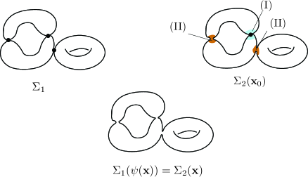
Figure 10. Part (I) and (II)

∎

We take the choice of ${\mathfrak{W}}^{(2)}$ as in Lemma 7.66. Let

$$[(\Sigma_{c},\vec{z}_{c}),u_{c}]\in\mathcal{U}(\epsilon(c);(\Sigma_{2},\vec{z}_{2}),u_{2},{\mathfrak{W}}^{(2)}).$$

By definition there exists $\vec{w}_{c}\subset\Sigma_{c}$, ${\bf x}_{c}\in\mathcal{V}_{(2)}(\epsilon_{c})$, a bi-holomorphic map

$$\phi_{c}:(\Sigma_{2}({\bf x}_{c}),\vec{z}_{2}({\bf x}_{c})\cup\vec{w}_{2}({\bf x}_{c}))\to(\Sigma_{c},\vec{z}_{c}\cup\vec{w}_{c}),$$

and $\delta_{c}$, such that the following holds.

1. The $C^{2}$ distance between $u_{2}$ and $u_{c}\circ\phi_{c}\circ\Phi_{2,{\bf x}_{c},\delta_{c}}$ is smaller than $o(c)$.

2. $d({\bf x}_{c},o)$ goes to zero as $c$ goes to infinity.

3. The map $u_{c}\circ\phi_{c}$ has diameter $<o(c)$ on $\Sigma_{2}({\bf x}_{c})\setminus{\rm Im}(\Phi_{2,{\bf x}_{c},\delta_{c}})$.

By Lemma 7.9 we may assume that $\delta_{c}\to 0$.

By Item (2) we have $\psi({\bf x}_{c})\in\mathcal{V}^{(1)}$ for large $c$ and an isomorphism

$$\tilde{\psi}_{{\bf x}_{c}}:(\Sigma_{2}({\bf x}_{c}),\vec{z}_{2}({\bf x}_{c})\cup\vec{w}_{2}({\bf x}_{c}))\to(\Sigma_{1}(\psi({\bf x}_{c})),\vec{z}_{1}(\psi({\bf x}_{c}))\cup\vec{w}_{1}(\psi({\bf x}_{c}))).$$

We put

$$\phi^{\prime}_{c}=\phi_{c}\circ(\tilde{\psi}_{{\bf x}_{c}})^{-1}.$$

By our choice of ${\mathfrak{W}}^{(2)}$, the next diagram commutes.

(7.73)

Moreover the $C^{2}$ distance between

$$u_{2}\circ\phi\circ\Phi_{1,{\bf x}_{2},\delta}\qquad\text{and}\qquad u_{1}$$

is smaller than $\epsilon$. Therefore (using Item (1) above also) for sufficiently large $c$ the $C^{2}$ distance between

$$u_{c}\circ\phi^{\prime}_{c}\circ\Phi_{1,\psi({\bf x}_{c}),\delta}\qquad\text{and}\qquad u_{1}$$

is smaller than $\epsilon$. Thus we checked Definition 7.8 (1). Definition 7.8 (2) is easy to check.

We will check Definition 7.8 (3). Let $C_{c}$ be a connected component of $\Sigma_{1}(\psi({\bf x}_{c}))\setminus{\rm Im}(\Phi_{1,\psi({\bf x}_{c}),\delta})$. There is a unique nodal point $p_{C_{c}}$ of $\Sigma_{1}$ which corresponds to $C_{c}$. (See Figure 11.) By our choice of ${\mathfrak{W}}^{(2)}$ one of the following holds.

1. $$C_{c}=\tilde{\psi}_{{\bf x}_{c}}(C_{c}^{\prime})$$

   for some connected component $C^{\prime}_{c}$ of $\Sigma_{2}({\bf x}_{c})\setminus\Phi_{2,{\bf x}_{c},\delta}$.

2. There is no nodal point corresponding to $p_{C_{c}}$ in $\Sigma_{2}$.

Suppose we are in case (a). By the commutativity of Diagram (7.73)

$$(u_{c}\circ\phi_{c})(C_{c})=(u_{c}\circ\phi^{\prime}_{c})(C_{c}^{\prime}).$$

Let

$$C^{\prime\prime}_{c}=C^{\prime}_{c}\setminus{\rm Im}(\Phi_{2,{\bf x}_{c},\delta_{c}}).$$

$C^{\prime\prime}_{c}$ is connected and hence the diameter of $(u_{c}\circ\phi^{\prime}_{c})(\tilde{\psi}_{{\bf x}_{c}}(C^{\prime\prime}_{c}))$ is smaller than $o(c)$.

On the other hand, we have

$$C^{\prime}_{c}\setminus C^{\prime\prime}_{c}\subseteq{\rm Im}(\Phi_{2,{\bf x}_{c},\delta_{c}}\setminus\Sigma_{2}(\delta)).$$

We define $D_{c}$ by:

$$C^{\prime}_{c}\setminus C^{\prime\prime}_{c}=(\Phi_{2,{\bf x}_{c},\delta_{c}})(D_{c}).$$

On $D_{c}$ the $C^{2}$ distance between

$$u_{2}\qquad\text{and}\qquad u_{c}\circ\phi_{c}\circ\Phi_{2,{\bf x}_{c},\delta_{c}}$$

is smaller than $o(c)$. On the other hand since $D_{c}$ is contained in a connected component of $\Sigma_{2}\setminus\Sigma_{2}(\delta)$ the diameter of $u_{2}(D_{c})$ is smaller than $\epsilon$.

Therefore the diameter of $(u_{c}\circ\phi^{\prime}_{c})(C_{c})$ is smaller than $\epsilon$ for sufficiently large $c$ in case (a).

Suppose we are in case (b). Note

$$u_{c}\circ\phi_{c}\circ\tilde{\psi}^{-1}_{{\bf x}_{c}}=u_{c}\circ\phi^{\prime}_{c}$$

holds on $C_{c}$. (In fact they both are defined there.) Therefore

$$\lim_{c\to\infty}{\rm Diam}(u_{c}\circ\phi^{\prime}_{c})(C_{c})=\lim_{c\to\infty}{\rm Diam}(u_{c}\circ\phi_{c})(\tilde{C}_{c})$$

where $\tilde{\psi}_{{\bf x}_{c}}(\tilde{C}_{c})=C_{c}$. Since we are in case (b), $\tilde{C}_{c}=\Phi_{2,{\bf x}_{c},\delta}(\hat{C}_{c})$ for some $\hat{C}_{c}\subset\Sigma_{2}(\delta_{c})$. We may assume that $\hat{C}_{c}$ lies in the $o(c)$ neighborhood of $\phi(C_{0,c})$, where $C_{0,c}$ is a component of $\Sigma_{1}({\bf x}_{2})\setminus{\rm Im}(\Phi_{1,{\bf x}_{2},\delta})$. Moreover on a neighborhood of $C_{0,c}$ the maps $u_{c}\circ\phi_{c}\circ\Phi_{2,{\bf x}_{c},\delta_{c}}$ converges to $u_{2}$. Thus

$${\rm Diam}(u_{c}\circ\phi_{c})(\tilde{C}_{c})\leq{\rm Diam}(u_{2}(C_{0,c}))+o(c).$$

By assumption ${\rm Diam}(u_{2}(C_{0,c}))<\epsilon$. So we conclude ${\rm Diam}(u_{c}\circ\phi_{c})(\tilde{C}_{c})<\epsilon$ for sufficiently large $c$.

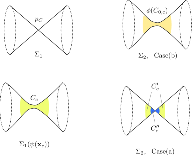
Figure 11. Estimate of the diameter of $u_{c}\circ\phi^{\prime}_{c}(C_{c})$

Thus, we have proved:

$$[(\Sigma_{c},\vec{z}_{c}),u_{c}]\in\mathcal{U}(\epsilon(c);(\Sigma_{1},\vec{z}_{1}),u_{1},{\mathfrak{W}}^{(1)}).$$

for sufficiently large $c$, as required. ∎

The proof of Proposition 7.36 in Case 5.

Using (Case 4) it suffices to show the following. For given strong stabilization data $({\mathfrak{W}}^{(1)},\vec{\mathcal{N}}_{1})$ at $\mathfrak{p}_{1}$ we can find strong stabilization data $({\mathfrak{W}}^{(2)},\vec{\mathcal{N}}_{2})$ at $\mathfrak{p}_{2}$ such that $\mathscr{J}_{12;\epsilon,\epsilon^{\prime}}$ exists. We will prove this statement below.

Since we fixed ${\mathfrak{W}}^{(1)}$, in particular we fixed $\vec{w}_{1}$. We take the universal family of deformation of $(\Sigma_{1},\vec{z}_{1}\cup\vec{w}_{1})$ and denote it by $\pi:\mathcal{C}_{(1)}\to\mathcal{V}_{(1)}$. (It comes with sections assigning marked points.)

Since $\mathfrak{p}_{2}=[\Sigma_{2},\vec{z}_{2}]$ is $\epsilon$ close to $\mathfrak{p}_{1}$ with respect to ${\mathfrak{W}}^{(1)}$ there exists ${\bf x}^{\prime}_{2}$ and $\vec{w}^{\,\prime}_{2}$ such that

$$\phi^{\prime}:(\Sigma_{1}({\bf x}^{\prime}_{2}),\vec{z}_{1}({\bf x}^{\prime}_{2})\cup\vec{w}_{1}({\bf x}^{\prime}_{2}))\cong(\Sigma_{2},\vec{z}_{2}\cup\vec{w}^{\,\prime}_{2}).$$

and it satisfies other conditions related to the maps $u_{1}$ and $u_{2}$. (See Definition 7.8.) It implies that $u_{2}(w^{\prime}_{2,j})$ is close to $u_{1}(w_{1,j})\in\mathcal{N}_{j}^{(1)}$. Since $u_{1}$ intersects transversaly with $\mathcal{N}_{j}^{(1)}$ and $u_{2}\circ\phi^{\prime}\circ\Phi_{1,{\bf x}^{\prime}_{2},\delta^{\prime}}$ is $C^{2}$ close to $u_{1}$, we can take $w_{2,j}$ such that $u_{2}(w_{2,j})\in\mathcal{N}_{j}^{(2)}$ and $d(w_{2,j},w^{\prime}_{2,j})<o(\epsilon)$. We take $(w_{2,1},\dots,w_{2,k})$ as our $\vec{w}_{2}$. Moreover we take $\mathcal{N}_{j}^{(2)}=\mathcal{N}_{j}^{(1)}$. There exists ${\bf x}_{2}$ and $\vec{w}_{2}$ such that

$$\phi:(\Sigma_{1}({\bf x}_{2}),\vec{z}_{1}({\bf x}_{2})\cup\vec{w}_{1}({\bf x}_{2}))\cong(\Sigma_{2},\vec{z}_{2}\cup\vec{w}_{2}).$$

In the same way as Lemma 7.66 we can find a system of analytic families of coordinates and trivialization data consisting ${\mathfrak{W}}^{(2)}$ so that

(7.74) $$\tilde{\psi}_{\bf x}\circ\Phi_{2,{\bf x},\delta^{\prime}}=\Phi_{1,\psi({\bf x}),\delta}\circ\Phi_{1,{\bf x}_{2},\delta}^{-1}\circ\phi^{-1}$$

holds on $\phi(\Phi_{1,{\bf x}_{2},\delta}(\Sigma_{1}(\delta))).$

We remark that the $C^{2}$ distance between

$$u_{2}\circ\phi\circ\Phi_{1,{\bf x}_{2},\delta}\qquad\text{and}\qquad u_{1}$$

is smaller than $o(\epsilon)$. Note this $C^{2}$ distance may not be smaller than $\epsilon$, since we changed $\vec{w}^{\,\prime}_{2}$ to $\vec{w}_{2}$. However the $C^{2}$ distance can certainly be estimated by $o(\epsilon)$.

Therefore in the same way as the proof of Lemma 7.27 we have

(7.75) $$\mathcal{U}(\epsilon^{\prime};(\Sigma_{2},\vec{z}_{2}),u_{2},{\mathfrak{W}}^{(2)})\subset\mathcal{U}(o(\epsilon);(\Sigma_{1},\vec{z}_{1}),u_{1},{\mathfrak{W}}^{(1)})$$

if $\epsilon^{\prime}$ is sufficiently small.

We define $\Psi:\Sigma_{1}(\delta)\to\Sigma_{2}$ by

(7.76) $$\Psi=(\Phi_{2,{\bf x},\delta^{\prime}})^{-1}\circ(\tilde{\psi}_{\bf x})^{-1}\circ\Phi_{1,{\psi}({\bf x}),\delta}=\phi\circ\Phi_{1,{\bf x}_{2},\delta}.$$

Here the right equality follows from (7.71). Compare (7.56). Here however contrary to (7.56) $\Psi$ is independent of ${\bf x}$.

We define

$$\Phi:L^{2}_{m+1}(\Sigma_{2}(\delta^{\prime}),X)\times\mathcal{V}_{2}(\epsilon^{\prime})\to L^{2}_{m+1}(\Sigma_{1}(\delta),X)\times\mathcal{V}_{1}(\epsilon)$$

by

(7.77) $$\Phi(F,{\bf x})=(F\circ\Psi,\psi({\bf x})).$$

Compare (7.58). Since $\Psi$ is independent of ${\bf x}$ and $\psi$ is smooth, the map $\Phi$ is smooth.

We define

(7.78) $$\mathcal{R}_{(1)}:\mathcal{V}^{(1)}_{\rm map}(\epsilon)\times\mathcal{V}_{(1)}(\epsilon)\to L^{2}_{m+1}(\Sigma_{1}(\delta),X)\times\mathcal{V}_{(1)}(\epsilon)$$

$$\mathcal{R}_{(2)}:\mathcal{V}^{(2)}_{\rm map}(\epsilon^{\prime})\times\mathcal{V}_{(2)}(\epsilon^{\prime})\to L^{2}_{m+1}(\Sigma_{2}(\delta^{\prime}),X)\times\mathcal{V}_{(2)}(\epsilon^{\prime})$$

by

(7.79) $$\mathcal{R}_{(i)}({\bf v},{\bf x})=(u^{i}_{{\bf v},{\bf x}}\circ\Phi^{(i)}_{1,{\bf x},\delta^{(i)}},{\bf x}).$$

Here $\delta^{(1)}=\delta$, $\delta^{(2)}=\delta^{\prime}$. Compare (7.57).

In the same way as the proof of Lemma 7.61 we can show that there exists $\tilde{\mathscr{J}}$ such that the next diagram commutes.

(7.80) $$\begin{CD}\mathcal{V}^{(2)}_{\rm map}(\epsilon^{\prime})\times\mathcal{V}_{(2)}(\epsilon^{\prime})@ >{\mathcal{R}_{(2)}}>>L^{2}_{m+1}(\Sigma_{2}(\delta^{\prime}),X)\times\mathcal{V}_{(2)}(\epsilon^{\prime})\\ @ VV{\tilde{\mathscr{J}}}V@ VV{\Phi}V\\ \mathcal{V}^{(1)}_{\rm map}(\epsilon)\times\mathcal{V}_{(1)}(\epsilon)@ >{\mathcal{R}_{(1)}}>>L^{2}_{m+1}(\Sigma_{1}(\delta),X)\times\mathcal{V}_{(1)}(\epsilon).\end{CD}$$

The commutativity of Diagram (7.80) implies that $\tilde{\mathscr{J}}$ is of $C^{n}$ class. $\tilde{\mathscr{J}}$ induce a map $\mathscr{J}_{12;\epsilon,\epsilon^{\prime}}$ in the same way as Lemma 7.62. Using the fact that $\#\vec{w}_{1}=\#\vec{w}_{2}$ we can show that $\mathscr{J}_{12;\epsilon,\epsilon^{\prime}}$ is a $C^{n}$ embedding in the same way as the proof of Lemma 7.63, that is, Case 1-1. The proof of Proposition 7.36 now complete. ∎

The proof of Proposition 7.36 and Lemma 7.27 is complete. We turn to the proof of Lemma 7.37.

Proof of Lemma 7.37.

Let ${\mathscr{L}}^{2}_{m+1}(\Sigma_{1}(\delta),X)$ be an $\epsilon_{0}$ neighborhood of $u_{1}$ in $L^{2}_{m+1}(\Sigma_{1}(\delta),X)$. We consider the direct product

(7.81) $${\mathscr{L}}^{2}_{m+1}(\Sigma_{1}(\delta),X)\times\mathcal{V}_{(1)}$$

and a bundle $\mathfrak{E}_{1}$ on it such that its total space is

(7.82) $$\mathfrak{E}_{1}=\{((\hat{u}^{\prime},{\bf x},V)\mid(\hat{u}^{\prime},{\bf x})\in(\ref{form770}),\,V\in L^{2}_{m}(\Sigma_{1}(\delta);(\hat{u}^{\prime})^{*}TX\otimes\Phi_{1,{\bf x},\delta}^{*}\Lambda^{01})\}$$

with obvious projection. $\mathfrak{E}_{1}\to{\mathscr{L}}^{2}_{m+1}(\Sigma_{1}(\delta),X)\times\mathcal{V}_{(1)}$.

Lemma 7.67.

If $m$ is larger than 10, then $\mathfrak{E}_{1}$ has a structure of smooth vector bundle and $\mathcal{G}_{1}$ acts on it.

Proof.

Let $(\hat{u}^{\prime},{\bf x})\in(\ref{form770})$. We put $\Phi_{1,{\bf x},\delta}(\Sigma_{1}(\delta))=\Sigma_{1}({\bf x})(\delta)$. There exists a canonical identification

$$L^{2}_{m}(\Sigma_{1}({\bf x})(\delta);(\hat{u}^{\prime})^{*}TX\otimes\Phi_{1,{\bf x},\delta}^{*}\Lambda^{01})\cong L^{2}_{m}(\Sigma_{1}(\delta);(u^{\prime})^{*}TX\otimes\Lambda^{01})$$

where $u^{\prime}=\hat{u}^{\prime}\circ\Phi_{1,{\bf x},\delta}^{-1}$. We defined

$$I_{\hat{u}^{\prime},{\bf x}}:L^{2}_{m}(\Sigma_{1}({\bf x})(\delta);(u^{\prime})^{*}TX\otimes\Lambda^{01})\to L^{2}_{m}(\Sigma_{1}(\delta);u_{1}^{*}TX\otimes\Lambda^{01}).$$

in (7.12). Combining them we obtain a bijection

(7.83) $$\mathfrak{E}_{1}\cong{\mathscr{L}}^{2}_{m+1}(\Sigma_{1}(\delta),X)\times\mathcal{V}_{(1)}\times L^{2}_{m}(\Sigma_{1}(\delta);u_{1}^{*}TX\otimes\Lambda^{01}).$$

We define $C^{\infty}$ structure of $\mathfrak{E}_{1}$ by this isomorphism. $\mathcal{G}_{1}$ invariance of this trivialization is immediate from definition. ∎

The vector space $E(\hat{u}^{\prime},{\bf x})$ is identified with a finite dimensional linear subspace of $L^{2}_{m+1}(\Sigma_{1}(\delta);u_{1}^{*}TX\otimes\Lambda^{01})$ by (7.8).

Lemma 7.68.

(7.84) $$\bigcup_{(\hat{u}^{\prime},{\bf x})\in(\ref{form770})}\{(\hat{u}^{\prime},{\bf x})\}\times E(\hat{u}^{\prime},{\bf x})$$

become a smooth subbundle of the right hand side of (7.83) by this identification.

Proof.

This is nothing but Proposition 7.14. ∎

We pull back the bundle in Lemma 7.68 by the $C^{n}$ embedding

$$V(\mathfrak{p}_{1};\epsilon;({\mathfrak{W}}^{(1)},\vec{\mathcal{N}}_{1}))\to\mathcal{V}_{\rm map}\times\mathcal{V}_{(1)}(\epsilon)\overset{\mathcal{R}_{(1)}}{\to}{\mathscr{L}}^{2}_{m+1}(\Sigma_{1}(\delta),X)\times\mathcal{V}_{(1)}$$

to obtain a (finite dimensional) vector bundle on $V(\mathfrak{p}_{1};\epsilon;({\mathfrak{W}}^{(1)},\vec{\mathcal{N}}_{1}))$ of $C^{n}$ class, which we write $\mathfrak{E}(\mathfrak{p}_{1};\epsilon;({\mathfrak{W}}^{(1)},\vec{\mathcal{N}}_{1}))$. $\mathcal{G}_{1}$ acts on it and the action is of $C^{n}$ class.

To complete the proof of Lemma 7.37 it suffices to show that $\mathfrak{E}(\mathfrak{p}_{1};\epsilon;({\mathfrak{W}}^{(1)},\vec{\mathcal{N}}_{1}))$ can be glued to give a vector bundle of $C^{n}$ class on $U(((\Sigma,\vec{z}),u);\epsilon_{2})$.

Suppose $\mathfrak{p}_{2}$ is $\epsilon$ close to $\mathfrak{p}_{1}$ with respect to ${\mathfrak{W}}^{(1)}$. We choose strong stabilization data $({\mathfrak{W}}^{(2)},\vec{\mathcal{N}}_{2})$ at $\mathfrak{p}_{2}$ (Definition 7.5).

Let $\mathscr{J}_{12;\epsilon,\epsilon^{\prime}}:V(\mathfrak{p}_{2};\epsilon^{\prime},({\mathfrak{W}}^{(2)},\vec{\mathcal{N}}_{2}))\to V(\mathfrak{p}_{1};\epsilon,({\mathfrak{W}}^{(1)},\vec{\mathcal{N}}_{1}))$ be the map we produced during the proof of Proposition 7.36. We show that there exists a canonical lift of this map to the fiber-wise linear map

(7.85) $$\widetilde{\mathscr{J}}_{12;\epsilon,\epsilon^{\prime}}:\mathfrak{E}(\mathfrak{p}_{2};\epsilon^{\prime};({\mathfrak{W}}^{(2)},\vec{\mathcal{N}}_{2}))\to\mathfrak{E}(\mathfrak{p}_{1};\epsilon;({\mathfrak{W}}^{(1)},\vec{\mathcal{N}}_{1})).$$

We take $e_{1},\dots,e_{d}$ a basis of $E((\Sigma,\vec{z}),u)$. Then a frame of $\mathfrak{E}(\mathfrak{p}_{1};\epsilon;{\mathfrak{W}}^{(1)})$ is given by

(7.86) $$e^{1}_{j}({\bf v},{\bf x}) =I_{\hat{u}^{\prime},{\bf x}}(I^{(1)}_{{\bf x}^{(1)}_{0},\phi^{(1)}_{0};((\Sigma^{\prime},\vec{z}^{\,\prime}),u^{\prime})}(g^{(1)}(\hat{u}^{\prime},{\bf x})_{*}(e_{j})))$$

$$\in L^{2}_{m+1}(\Sigma_{1}(\delta);u_{1}^{*}TX\otimes\Lambda^{01})$$

in (7.48). Here we write $I^{(1)}_{{\bf x}^{(1)}_{0},\phi^{(1)}_{0};((\Sigma^{\prime},\vec{z}^{\,\prime}),u^{\prime})}$ and $g^{(1)}(\hat{u}^{\prime},{\bf x})_{*}(e_{j}))$ to indicate that they are associated to $({\mathfrak{W}}^{(1)},\vec{\mathcal{N}}_{1})$. Note $({\bf x}_{0},\phi_{0})=(\psi({\bf x}),\tilde{\psi}|_{\Sigma(\psi({\bf x}))})$, $(\Sigma^{\prime},\vec{z}^{\,\prime})=(\Sigma_{1}({\bf x}),\vec{z}_{1}({\bf x}))$ and

$$u^{\prime}=u^{1}_{{\bf v},{\bf x}}:\Sigma_{1}({\bf x})(\delta)\to X,\qquad\hat{u}^{\prime}=u^{\prime}\circ\Phi_{1,{\bf x},\delta}=u^{1}_{{\bf v},{\bf x}}\circ\Phi_{1,{\bf x},\delta}:\Sigma_{1}(\delta)\to X.$$

$e^{1}_{j}({\bf v},{\bf x})$ is a $C^{n}$ frame of $\mathfrak{E}(\mathfrak{p}_{1};\epsilon;({\mathfrak{W}}^{(1)},\vec{\mathcal{N}}_{1}))$ since it is a pull back of $C^{\infty}$ frame of the bundle (7.68). Note (7.86) depends on $\mathfrak{p}_{1}$ and $({\mathfrak{W}}^{(1)},\vec{\mathcal{N}}_{1})$ but is independent of the various choices we made in Subsection 7.4. (Those choices are used to prove the smoothness of right hand side.)

When we use $\mathfrak{p}_{2}$ and $({\mathfrak{W}}^{(2)},\vec{\mathcal{N}}_{2})$, and $({\bf v}^{\prime},{\bf x}^{\prime})\in\mathcal{V}^{(2)}_{\rm map}\times\mathcal{V}_{(2)}(\epsilon^{\prime})$ we put

$$u^{\prime\prime}=u^{2}_{{\bf v}^{\prime},{\bf x}^{\prime}}:\Sigma_{2}({\bf x}^{\prime})(\delta^{\prime})\to X,\qquad\hat{u}^{\prime\prime}=u^{\prime\prime}\circ\Phi_{2,{\bf x}^{\prime},\delta^{\prime}}=u^{2}_{{\bf v}^{\prime},{\bf x}^{\prime}}\circ\Phi_{2,{\bf x}^{\prime},\delta}:\Sigma_{2}(\delta^{\prime})\to X.$$

Suppose

$$({\bf v}^{\prime},{\bf x}^{\prime})={\mathscr{J}}_{12;\epsilon,\epsilon^{\prime}}({\bf v},{\bf x}).$$

Then $\psi_{1}({\bf x})=\psi_{2}({\bf x}^{\prime})$. Note $\psi_{1}$ in the left hand side is the map $\psi$ obtained from the deformation theory of $\Sigma_{1}$ and $\psi_{2}$ in the right hand side is the map $\psi$ obtained from the deformation theory of $\Sigma_{2}$. It induces an isomorphism

$$(\tilde{\psi}_{2}|_{\Sigma(\psi_{2}({\bf x}^{\prime}))})^{-1}\circ\tilde{\psi}_{1}|_{\Sigma(\psi_{1}({\bf x}))}:(\Sigma_{1}({\bf x}),\vec{z}_{1}({\bf x}))\cong(\Sigma_{2}({\bf x}^{\prime}),\vec{z}_{2}({\bf x}^{\prime}))$$

such that

$$u^{\prime\prime}\circ(\tilde{\psi}|_{\Sigma(\psi_{2}({\bf x}^{\prime}))})^{-1}\circ\tilde{\psi}|_{\Sigma(\psi_{1}({\bf x}))}=u^{\prime}.$$

Therefore the frame $e^{2}_{j}({\bf v}^{\prime},{\bf x}^{\prime})$ is given by

$$\left(\widetilde{\mathscr{J}}_{12;\epsilon,\epsilon^{\prime}}(e^{2}_{j})\right)({\bf v},{\bf x})=(I_{\hat{u}^{\prime},{\bf x}}\circ(I_{\hat{u}^{\prime\prime},{\bf x}^{\prime}})^{-1})(e^{1}_{j}({\bf v},{\bf x}))$$

In the same way as Subsection 7.4 we can write the right hand side using local coordinates and prove that $\widetilde{\mathscr{J}}_{12;\epsilon,\epsilon^{\prime}}$ is of $C^{n}$ class. ∎

Proof of Lemma 7.38.

It remains to prove that the Kuranishi map $s$ is of $C^{n}$ class. We use the trivialization (7.83) and regard $\mathfrak{E}(\mathfrak{p}_{1};\epsilon;{\mathfrak{W}}^{(1)})$ as a subbundle of the trivial bundle (the right hand side of (7.83)).

For ${\bf x}\in\mathcal{V}_{(1)}$ we take the complex structure of $\Sigma_{1}({\bf x})$ and pull it back to $\Sigma_{1}(\delta)$ by $\Phi_{1,{\bf x},\delta}$. We thus obtain a $(\hat{u}^{\prime},{\bf x})$ parametrized family of complex structures on $\Sigma_{1}(\delta)$, which we denote by $j_{(\hat{u}^{\prime},{\bf x})}$. This is a family of complex structures depending smoothly on $(\hat{u}^{\prime},{\bf x})$. By definition

(7.87) $$s(\hat{u}^{\prime},(\hat{u}^{\prime},{\bf x}))$$

$$=\overline{\partial}_{j_{(\hat{u}^{\prime},{\bf x})}}(\hat{u}^{\prime})$$

$$=\left(A^{i}_{\sigma}(\hat{u}^{\prime},{\bf x})(\hat{u}^{\prime}(z_{\sigma}))\frac{\partial\hat{u}^{\prime}_{i}}{\partial x_{\sigma}}+B^{i}_{\sigma}(\hat{u}^{\prime},{\bf x})(\hat{u}^{\prime}(z_{\sigma}))\frac{\partial\hat{u}^{\prime}_{i}}{\partial y_{\sigma}}\right)\partial^{i}_{\sigma}\otimes d\overline{z}_{\sigma}.$$

on a (sufficiently small) coordinate chart $W_{\sigma}$ on $\Sigma_{1}(\delta)$ and $\Omega_{\sigma}$ of $X$ containing a neighborhood of $u_{1}(W_{\sigma})$. Here $z_{\sigma}=x_{\sigma}+\sqrt{-1}y_{\sigma}$ is a complex coordinate of $W_{\sigma}$ and $\partial^{i}_{\sigma}$ is a frame of the complex tangent bundle $TX$ on $\Omega_{\sigma}$. $A^{i}_{\sigma}$ and $B^{i}_{\sigma}$ are smooth functions

$$\mathcal{V}_{\rm map}\times\mathcal{V}_{(1)}(\epsilon)\times\Omega_{\sigma}\to{\mathbb{C}}.$$

Therefore the Kuranshi map $s$ is of $C^{\infty}$ class in terms of this trivialization. ∎

The proof of Proposition 6.15 is complete. In fact, Proposition 6.15 (5) holds at $[(\Sigma,\vec{z}),u]$ by Condition 4.6 (2) and hence holds everywhere by taking $\epsilon_{1}$ small. ∎

7.6. From $C^{n}$ structure to $C^{\infty}$ structure

This subsection is similar to [FOOO6, Section 26] and [FOOO12, Section 12].

So far we have constructed a $G$-equivariant Kuranishi chart of $C^{n}$ class for any $n$. In this subsection, we show how we obtain one in $C^{\infty}$ class.

We consider the embedding

$$\mathcal{R}_{(1),m}:\mathcal{V}^{(1)}_{\rm map}(\epsilon)\times\mathcal{V}_{(1)}(\epsilon)\to L^{2}_{m+1}(\Sigma_{1}(\delta),X)\times\mathcal{V}_{(1)}(\epsilon)$$

as in (7.57) and (7.79). We put $m$ in the suffix to specify the Hilbert space $L^{2}_{m+1}$ we use. We proved that this is a smooth embedding of $C^{n}$ class if $m>n+10$ and $\epsilon<\epsilon_{m}$. We fix $\epsilon_{0}<\epsilon_{10}$ and show the next lemma.

Lemma 7.69.

The image of

$$\mathcal{R}_{(1),10}:\mathcal{V}^{(1)}_{\rm map}(\epsilon_{0})\times\mathcal{V}_{(1)}(\epsilon_{0})\to L^{2}_{11}(\Sigma_{1}(\delta),X)\times\mathcal{V}_{(1)}(\epsilon_{0})$$

is contained in $C^{k}(\Sigma_{1}(\delta),X)\times\mathcal{V}_{(1)}(\epsilon_{0})$ for any $k$ and is a smooth submanifold of $L^{2}_{11}(\Sigma_{1}(\delta),X)\times\mathcal{V}_{(1)}(\epsilon_{0})$ of $C^{\infty}$ class.

Proof.

By elliptic regularity $u_{{\bf v},{\bf x}}$ is a smooth map. Moreover $\Phi_{1,{\bf x},\delta}$ is a smooth map. Therefore by definition the image of $\mathcal{R}_{(1),m}$ is contained in $C^{\infty}(\Sigma_{1}(\delta),X)\times\mathcal{V}_{(1)}(\epsilon_{0})$.

Remark 7.70.

We remark that the image of $\mathcal{R}_{(1),m}$ coincides with the image of $\mathcal{R}_{(1),m^{\prime}}$ in a neighborhood of $((\Sigma_{1},\vec{z}_{1}\cup\vec{w}_{1}),u_{1})$.

In fact they coincides with the set of all the pairs $(u^{\prime}\circ\Phi_{a,{\bf x},\delta},{\bf x})$, where $u^{\prime}:\Sigma_{1}({\bf x})\to X$ such that $\overline{\partial}u^{\prime}\in E((\Sigma_{1}({\bf x}),\vec{z}_{1}({\bf x})),u^{\prime})$ and $(\Sigma_{1}({\bf x}),\vec{z}_{1}({\bf x})\cup\vec{w}_{1}({\bf x}),u^{\prime})$ is $\epsilon$-close to $(\Sigma_{1},\vec{z}_{1}\cup\vec{w}_{1},u_{1})$. (This is a consequence of Lemma 7.23.)

We put

$$\widehat{\mathcal{R}}_{(1)}^{k}:\mathcal{V}^{(1)}_{\rm map}(\epsilon_{0})\times\mathcal{V}_{(1)}(\epsilon_{0})\to C^{k}(\Sigma_{1}(\delta),X)\times\mathcal{V}_{(1)}(\epsilon_{0})$$

Note the map

$$L^{2}_{m}(\Sigma_{1}(\delta),X)\times\mathcal{V}_{(1)}(\epsilon_{0})\to C^{k}(\Sigma_{1}(\delta),X)\times\mathcal{V}_{(1)}(\epsilon_{0})$$

is a smooth embedding for $k>m+10$. In fact the first factor is a smooth embedding between Banach manifolds and the second factor is the identity map. It implies that the image ${\mathcal{R}}_{(1),10}(\mathcal{V}^{(1)}_{\rm map}(\epsilon_{m})\times\mathcal{V}_{(1)}(\epsilon_{m}))$ is a submanifold of $C^{n}$ class if $n>m+10$. The issue is $\epsilon_{m}\to 0$ as $m\to\infty$. So to prove the lemma we consider also the charts centered at various points altogether.

Let $\mathfrak{p}_{2}\in\mathcal{V}^{(1)}_{\rm map}(\epsilon_{0})\times\mathcal{V}_{(1)}(\epsilon_{0})$. We fixed a stabilization data ${\mathfrak{W}}^{(1)}$ at $\mathfrak{p}_{1}$. We take a stabilization data ${\mathfrak{W}}^{(2)}$ at $\mathfrak{p}_{2}$ as in Case 5 of the proof of Proposition 7.36. We have a commutative diagram similar to (7.80):

(7.88) $$\begin{CD}\mathcal{V}^{(2)}_{\rm map}(\epsilon_{m})\times\mathcal{V}_{(2)}(\epsilon_{m})@ >{\mathcal{R}_{(2)}}>>L^{2}_{m+1}(\Sigma_{2}(\delta_{m}),X)\times\mathcal{V}_{(2)}(\epsilon_{m})\\ @ VV{\tilde{\mathscr{J}}}V@ VV{\Phi}V\\ \mathcal{V}^{(1)}_{\rm map}(\epsilon_{0})\times\mathcal{V}_{(1)}(\epsilon_{0})@ >{\widehat{\mathcal{R}}^{k}_{(1)}}>>C^{k}(\Sigma_{1}(\delta),X)\times\mathcal{V}_{(1)}(\epsilon_{0})\end{CD}$$

with

(7.89) $$\Phi(F,{\bf x})=(F\circ\phi\circ\Phi_{1,{\bf x}_{2},\delta},\psi({\bf x})).$$

(See (7.76) and (7.77).) The map in the right vertical arrow is of $C^{\infty}$ class since $F\mapsto F\circ\phi\circ\Phi_{1,{\bf x}_{2},\delta}$ with $\phi\circ\Phi_{1,{\bf x}_{2},\delta}$ is a smooth map independent of ${\bf x}$ and $\psi$ is smooth. It follows that the image of ${\mathcal{R}}_{(1),10}$ is of $C^{n}$ class at $\mathfrak{p}_{2}$ for $m>n+k+10$. Since this holds for any $\mathfrak{p}_{2}$ and $m$, Lemma 7.69 follows. ∎

We regard $\mathcal{V}^{(1)}_{\rm map}(\epsilon_{0})\times\mathcal{V}_{(1)}(\epsilon_{0})$ as a manifold of $C^{\infty}$ class so that the embedding $\mathcal{R}_{(1),10}$ becomes an embedding of $C^{\infty}$ class. Note this $C^{\infty}$ structure is different from previously defined one, which is the direct product structure using Definition 7.19. They coincide each other at the origin $\mathfrak{p}_{1}$ and also the underlying $C^{1}$ structure coincides everywhere. We call this $C^{\infty}$ structure the new $C^{\infty}$ structure.

We remark that

$$V(\mathfrak{p}_{1};\epsilon_{0},({\mathfrak{W}}^{(1)},\vec{\mathcal{N}}_{1}))=\{({\bf v},{\bf x})\mid u^{1}_{{\bf v},{\bf x}}(w_{1,j}({\bf x}))\in\mathcal{N}_{j}^{(1)},j=1,\dots,k_{1}\}.$$

by definition. We consider the next commutative diagram.

(7.90)

where $m>k+10$. Here the two maps to $X$ appearing in Diagram (7.90) is given by $(\hat{u}^{\prime},{\bf x})\mapsto\hat{u}^{\prime}((\Phi_{i,{\bf x},\delta})^{-1}(w_{i,j}({\bf x})))$. Note this map

$$C^{k}(\Sigma_{2}(\delta),X)\times\mathcal{V}_{(2)}(\epsilon_{m})\to X$$

is of $C^{k}$ class. Therefore the composition

$$\mathcal{V}^{(1)}_{\rm map}(\epsilon_{0})\times\mathcal{V}_{(1)}(\epsilon_{0})\to L^{2}_{11}(\Sigma_{1}(\delta),X)\times\mathcal{V}_{(1)}(\epsilon_{0})\to X$$

(which is nothing but the map $({\bf v},{\bf x})\mapsto u^{1}_{{\bf v},{\bf x}}(w_{1,j}({\bf x}))$ is of $C^{k}$ class with respect to the new $C^{\infty}$ structure of $\mathcal{V}^{(1)}_{\rm map}(\epsilon_{0})\times\mathcal{V}_{(1)}(\epsilon_{0})$ at $\mathfrak{p}_{2}$. (Here we use the fact that $\Phi$ is of $C^{\infty}$ class, $\tilde{\mathscr{J}}$ is an open embedding of $C^{k}$ class, and the commutativity of the Diagram (7.90).)

Since this holds for any $\mathfrak{p}_{2}$ and $k$, the submanifold $V(\mathfrak{p}_{1};\epsilon_{0},({\mathfrak{W}}^{(1)},\vec{\mathcal{N}}_{1}))$ is a submanifold of $C^{\infty}$ class of $\mathcal{V}^{(1)}_{\rm map}(\epsilon_{0})\times\mathcal{V}_{(1)}(\epsilon_{0})$ equipped with the new $C^{\infty}$ structure.

We thus defined a $C^{\infty}$ structure on $V(\mathfrak{p}_{1};\epsilon_{0},({\mathfrak{W}}^{(1)},\vec{\mathcal{N}}_{1}))$. Here $\epsilon_{0}$ is $\mathfrak{p}_{1}$ dependent. So we write $V(\mathfrak{p}_{1};\epsilon_{\mathfrak{p}_{1}},({\mathfrak{W}}^{(1)},\vec{\mathcal{N}}_{1}))$ from now on.

We next show that the coordinate change

$$\mathscr{J}_{12;\epsilon_{\mathfrak{p}_{1}},\epsilon_{\mathfrak{p}_{2}}}:V(\mathfrak{p}_{2};\epsilon_{\mathfrak{p}_{2}},({\mathfrak{W}}^{(2)},\vec{\mathcal{N}}_{2}))\to V(\mathfrak{p}_{1};\epsilon_{\mathfrak{p}_{1}},({\mathfrak{W}}^{(1)},\vec{\mathcal{N}}_{1}))$$

is of $C^{\infty}$ class with respect to the new $C^{\infty}$ structure.

Let $\mathfrak{p}_{3}\in V(\mathfrak{p}_{2};\epsilon_{\mathfrak{p}_{2}},({\mathfrak{W}}^{(2)},\vec{\mathcal{N}}_{2}))$ be an arbitrary point. It suffices to prove that $\mathscr{J}_{12;\epsilon_{\mathfrak{p}_{1}},\epsilon_{\mathfrak{p}_{2}}}$ is of $C^{\infty}$ class at $\mathfrak{p}_{3}$. We take two strong stabilization data $({\mathfrak{W}}^{(3,1)},\vec{\mathcal{N}}_{3,1})$ and $({\mathfrak{W}}^{(3,2)},\vec{\mathcal{N}}_{3,2})$ at $\mathfrak{p}_{3}$ as follows.

1. $\mathfrak{p}_{2},({\mathfrak{W}}^{(2)},\vec{\mathcal{N}}_{2})$ and $({\mathfrak{W}}^{(3,2)},\vec{\mathcal{N}}_{3,2})$ are as in Case 5 of the proof of Proposition 7.36.

2. $\mathfrak{p}_{1},({\mathfrak{W}}^{(1)},\vec{\mathcal{N}}_{1})$ and $({\mathfrak{W}}^{(3,1)},\vec{\mathcal{N}}_{3,1})$ are as in in Case 5 of the proof of Proposition 7.36.

We consider the next diagram.

(7.91) $$\!\!\!\!\!\!\!\!\!\!\!\!\!\!\!\!\!\!\!\!\!\!\!\!\begin{CD}V(\mathfrak{p}_{3};\epsilon^{\prime},({\mathfrak{W}}^{(3,2)},\vec{\mathcal{N}}_{3,2}))@ >{\mathscr{J}_{23;\epsilon_{\mathfrak{p}_{2}},\epsilon^{\prime}}}>>V(\mathfrak{p}_{2};\epsilon_{\mathfrak{p}_{2}},({\mathfrak{W}}^{(2)},\vec{\mathcal{N}}_{2}))\\ @ VV{\mathscr{J}_{33;\epsilon,\epsilon^{\prime}}}V@ VV{\mathscr{J}_{12;\epsilon_{\mathfrak{p}_{1}},\epsilon_{\mathfrak{p}_{2}}}}V\\ V(\mathfrak{p}_{3};\epsilon,({\mathfrak{W}}^{(3,1)},\vec{\mathcal{N}}_{3,1}))@ >{\mathscr{J}_{13;\epsilon_{\mathfrak{p}_{1}},\epsilon}}>>V(\mathfrak{p}_{1};\epsilon_{\mathfrak{p}_{1}},({\mathfrak{W}}^{(1)},\vec{\mathcal{N}}_{1})).\end{CD}$$

The commutativity of Diagram (7.91) up to $\mathcal{G}_{1}$ action is a consequence of (7.50).

By the proof of Lemma 7.69 and the definition of the $C^{\infty}$ structures, the horizontal arrows are smooth at the origin $\mathfrak{p}_{3}$. Therefore it suffices to prove that the left vertical arrow is of $C^{\infty}$ class at $\mathfrak{p}_{3}$.

This is actually a consequence of the proof of Proposition 7.36. To carry out the proof of Proposition 7.36 we take $L^{2}_{m+2n+1}$ space for ${\mathfrak{W}}^{(3,2)}$ and $L^{2}_{m+n+1}$ space for ${\mathfrak{W}}^{(3,1)}$. Then the coordinate change $\mathscr{J}_{33;\epsilon,\epsilon^{\prime}}$ is of $C^{n}$ class if $m>n+10$. Therefore $\mathscr{J}_{12;\epsilon_{\mathfrak{p}_{1}},\epsilon_{\mathfrak{p}_{2}}}$ is of $C^{n}$ class for any $n$ at $\mathfrak{p}_{3}$. So it is of $C^{\infty}$ class at $\mathfrak{p}_{3}$. (We use Remark 7.70 here with ${\mathfrak{p}_{1}}$ replaced by ${\mathfrak{p}_{3}}$.)

We thus proved that our smooth structures on $V(\mathfrak{p}_{1};\epsilon_{0},({\mathfrak{W}}^{(1)},\vec{\mathcal{N}}_{1}))$ can be glued to give a smooth structure on $U(((\Sigma,\vec{z}),u);\epsilon_{2})$.

The proof that we can define a smooth structure on our obstruction bundle $E(((\Sigma,\vec{z}),u);\epsilon_{2})$ is similar. Note the new $C^{\infty}$ structure on $V(\mathfrak{p}_{1};\epsilon_{0},({\mathfrak{W}}^{(1)},\vec{\mathcal{N}}_{1}))$ is defined so that the map

$$V(\mathfrak{p}_{1};\epsilon_{0},({\mathfrak{W}}^{(1)},\vec{\mathcal{N}}_{1}))\to\mathcal{V}^{(1)}_{\rm map}(\epsilon_{0})\times\mathcal{V}_{(1)}(\epsilon_{0})\to L^{2}_{11}(\Sigma_{1}(\delta),X)\times\mathcal{V}_{(1)}(\epsilon_{0})$$

is an embedding of $C^{\infty}$ class. Therefore we can define a smooth structure on $\mathfrak{E}(\mathfrak{p}_{1};\epsilon;{\mathfrak{W}}^{(1)})$ so that the trivialization (7.83) is a trivialization of $C^{\infty}$ class.

The proof that the map

$$\widetilde{\mathscr{J}}_{12;\epsilon_{\mathfrak{p}_{1}},\epsilon_{\mathfrak{p}_{2}}}:\mathfrak{E}(\mathfrak{p}_{1};\epsilon;({\mathfrak{W}}^{(1)},\vec{\mathcal{N}}_{1}))\to\mathfrak{E}(\mathfrak{p}_{2};\epsilon;({\mathfrak{W}}^{(2)},\vec{\mathcal{N}}_{2})).$$

(7.85) is of $C^{\infty}$ class is the same as the proof that ${\mathscr{J}}_{12;\epsilon_{\mathfrak{p}_{1}},\epsilon_{\mathfrak{p}_{2}}}$ is of $C^{\infty}$ class.

The smoothness of the Kuranishi map is immediate from (7.87).

The proof of Lemma 7.38 is now complete. ∎

8. Convex function and Riemannian center of Mass: Review

This section is a review of convex function and center of mass technique, which are classical topics in Riemannian geometry. (See [GK].) We include this review in this paper since this topic is not so familiar among the researchers of pseudo holomorphic curve, Gromov-Witten theory, or Floer homology. (For example Proposition 8.8 is hard to find in the literature though this proposition is certainly regarded as ‘obvious’ by experts.)

Let $M$ be a Riemannian manifold. We use Levi-Civita connection $\nabla$. A geodesic is a map $\ell:[a,b]\to M$ such that $\nabla_{\dot{\ell}}\dot{\ell}=0$ and $\|\dot{\ell}(t)\|$ is a nonzero constant.

Definition 8.1.

A function $f:M\to{\mathbb{R}}$ is said to be convex if for any geodesic $\ell:[a,b]\to M$ we have

(8.1) $$\frac{d^{2}}{dt^{2}}(f\circ\ell)\geq 0.$$

$f$ is said to be strictly convex if the strict inequality $>$ holds.

In case

$$\frac{d^{2}}{dt^{2}}(f\circ\ell)\geq c>0$$

for all geodesic $\ell$ with $\|\dot{\ell}\|=1$, we say $f$ is $c$-strictly convex.

The usefulness of strict convex function for our purpose is the following:

Lemma 8.2.

Let $f:M\to{\mathbb{R}}$ be a strictly convex function. Suppose $f$ assumes its local minimum at both $p,q\in M$. We also assume that there exists a geodesic joining $p$ and $q$. Then $p=q$.

Proof.

This is an immediate consequence from the fact if $h:[a,b]\to{\mathbb{R}}$ is a strictly convex function and $h$ assume local minimum at both $a,b$ then $a=b$. ∎

A typical example of a convex function is the Riemannian distance. We denote by $d_{M}:M\times M\to{\mathbb{R}}_{\geq 0}$ the Riemannian distance function. Let $U\subset M$ be a relatively compact open subset.

Lemma 8.3.

There exists $\epsilon>0$ such that on

$$\{(p,q)\mid p,q\in U,d_{M}(p,q)<\epsilon\}$$

the function

$$(p,q)\mapsto d_{M}(p,q)^{2}$$

is smooth and convex.

This is a standard fact in Riemannian geometry. Note this function $(p,q)\mapsto d_{M}(p,q)^{2}$ is not strictly convex. However for a fixed $q$, the function $p\mapsto d_{M}(p,q)^{2}$ is strictly convex. We need to restrict the direction for the positivity of the second derivative of $(p,q)\mapsto d_{M}(p,q)^{2}$. See the proof of Proposition 8.8 below.

We use the next lemma also.

Lemma 8.4.

Let $N$ be an oriented manifold with volume form $\Omega_{N}$ and $f:M\times N\to{\mathbb{R}}$ a smooth function. Suppose that for each $y\in N$ $x\mapsto f(x,y)$ is convex and for each $x_{0}\in M$ there exists $y$ such that $x\mapsto f(x,y)$ is strictly convex in a neighborhood of $x_{0}$. Then the function $F:M\to{\mathbb{R}}$

$$F(x)=\int_{y\in N}f(x,y)\Omega_{N}$$

is strictly convex.

The proof is obvious.

For our application we need to show convexity of certain functions induced by a distance function. We use Proposition 8.8 for this purpose. We also need to ensure uniformity of various constants obtained. We use a version of boundedness of geometry for this purpose. The next definition is a bit extravagant for our purpose. However the situation we use certainly satisfies this condition.

Definition 8.5.

A family $\{(N_{b},K_{b})\mid b\in\mathcal{B}\}$ of a pair of Riemannian manifolds $N_{b}$ and its compact subsets $K_{b}$ is said to be of bounded geometry in all degree if there exists $\mu>0$ and $C_{k}$ ($k=0,1,\dots,$) with the following properties.

1. The injectivity radius is greater than $\mu$ at all points $x\in K_{b}\subset N_{b}$.

2. Moreover the metric ball of radius $\mu$ centered at $x\in K_{b}\subset N_{b}$ are relatively compact in $N_{b}$.

3. We have estimate

   $$\|\nabla^{k}R^{N_{b}}\|\leq C_{k},$$

   for $k=0,1,2,\dots$. Here $R^{N_{b}}$ is the Riemann curvature tensor of ${N_{b}}$ and $\nabla$ is the Levi-Civita connection. The inequality holds everywhere (point-wise) on ${N_{b}}$.

When we need to specify $\mu$, $\{C_{k}\}$ we say bounded geometry in all degree by $\mu$, $\{C_{k}\}$.

Remark 8.6.

We consider a pair $(N_{b},K_{b})$ rather than a single Riemannian manifold $N_{b}$, in order to include the case when our Riemannian manifold is not complete.

We use geodesic coordinate $\exp:B_{\mu/2,x}{N_{b}}\to{N_{b}}$. Here $B_{\mu/2,x}{N_{b}}$ is the metric ball of radius $\mu/2$ centered at $0$ in the tangent space $T_{x}{N_{b}}$. Item (3) implies that the coordinate change of geodesic coordinate has uniformly bounded $C^{k}$ norm for any $k$.

Definition 8.7.

Let $\{(N_{b},K_{b})\mid b\in\mathcal{B}\}$ be as in Definition 8.5 and $M$ a Riemannian manifold. Let $\delta<\mu/2$. A family of smooth maps $f_{b}:N_{b}\to M$ is said to have uniform $C^{k}$ norm on the $\delta$ neighborhood of $K_{b}$ if the composition

(8.2) $$f_{b}\circ\exp:B_{\delta,x}{N_{b}}\to M$$

has uniformly bounded $C^{k}$ norm for $x\in K_{b}$. Here we regard $B_{\delta,x}{N_{b}}=\{V\in T_{x}N_{b}\mid\|V\|<\delta\}$ as an open subset of the Euclid space by isometry.

When we specify the $C^{k}$ bound, we say has uniformly bounded $C^{k}$ norm $\leq B_{k}$. It means that the $C^{k}$ norm of (8.2) is not greater than $B_{k}$.

Proposition 8.8.

Given $\mu$, $\{C_{k}\}$, $B$, $\delta$, $\rho$ there exists $\epsilon$ with the following properties.

Let $\{(N_{b},K_{b})\mid b\in\mathcal{B}\}$ have bounded geometry in all degree by $\mu$, $\{C_{k}\}$ and $f_{b},g_{b}:N_{b}\to M$ be a pair of smooth maps such that they have uniform $C^{2}$ bound by $B$ on $\delta$ neighborhood of $K_{b}$. Suppose

$$d_{M}(f_{b}(x),g_{b}(x))\leq\epsilon$$

holds on $\delta$ neighborhoods of $K_{b}$. Moreover we assume

$$d_{TM}(D_{V}f_{b},D_{V}g_{b})\geq\rho$$

for all $V\in T_{x}N_{b}$, $\|V\|=1$, $d(x,K_{b})<\delta$. (Here $d$ is the Riemannian distance in the tangent bundle of $M$.)

Then the function

(8.3) $$x\mapsto d_{M}(f_{b}(x),g_{b}(x))^{2}$$

on $K_{b}$ is strictly convex. Moreover there exists $\sigma$ depending only on $\mu$, $\{C_{k}\}$, $B$, $\delta$, $\rho$ such that (8.3) is $\sigma$-strictly convex.

Proof.

Let $\ell:[-c,c]\to B_{\delta}K_{b}=\{x\in N_{b}\mid d_{N_{b}}(x,K_{b})<\delta\}$ be a geodesic of unit speed. We put $\gamma_{b}(t)=(f_{b}(\ell(t)),g_{b}(\ell(t))$. Note

$$({\rm Hess}h)(V,V^{\prime})=\nabla_{V}\nabla_{V}^{\prime}h-\nabla_{\nabla_{V}V^{\prime}}h$$

is a symmetric 2 tensor. If $h=d_{M}^{2}$ then

$$({\rm Hess}\,d_{M}^{2})(V,V)\geq\sigma^{\prime}$$

if $V=(V_{1},V_{2})\in T_{(p,q)}M^{2}$, $\|V\|=1$, $d_{M}(p,q)<\epsilon_{1}$ and $d_{TM}(V_{1},V_{2})\geq\rho$. Therefore

$$\frac{d^{2}}{dt}(d_{M}^{2}\circ\gamma_{b})\geq C\rho-C\nabla_{\nabla_{\dot{\gamma_{b}}}\dot{\gamma_{b}}}d_{M}^{2}.$$

The second term can be estimated by

$$C|d_{M}||\nabla d_{M}|\leq C\epsilon_{1}.$$

The proposition follows. ∎

We also use the following lemma in Subsection 7.4.

Lemma 8.9.

Let $\pi:M\to N$ be a smooth fiber bundle on an open subset of a Hilbert space. We assume that the fibers are finite dimensional and take a smooth family of Riemannian metrics of the fibers.

Let $f:M\to{\mathbb{R}}$ be a smooth function. We assume:

1. The restriction of $f$ to the fibers are strictly convex.

2. The minimum of the restriction of $f$ to the fibers $\pi^{-1}(x)$ is attained at the unique point $g(x)\in\pi^{-1}(x)$ for each $x\in N$.

Then the map $g:N\to M$ is smooth.

Proof.

The proof of continuity of $g$ is an exercise of general topology, which we omit.

Let ${\rm KerD\pi}\subset TM$ be the subbundle consisting of the vectors of vertical direction. We define a section of its dual ${\rm KerD\pi}^{*}$ by

$$\nabla^{\rm vert}f:y\mapsto(V\mapsto V(f)).$$

Here $y\in M$, $V\in{\rm KerD_{y}\pi}\subset T_{y}M$. By assumption $(\nabla^{\rm vert}f)(y)=0$ if and only if $y=g(x)$ for $x=\pi(y)$.

The differential of $\nabla^{\rm vert}f$ at $g(x)$ is the Hessian of $f|_{\pi^{-1}(x)}$ at $x$ and so is non-degenerate by strict convexity of $f|_{\pi^{-1}(x)}$.

The smoothness of $g$ now is a consequence of implicit function theorem. ∎

References

- [ALR] A. Adem, J. Leida and Y. Ruan, Orbifolds and Stringy Topology, Cambridge Tracts in Math. 171, Cambridge University Press, Cambridge, 2007.
- [ACG] E. Arbarello, M. Cornalba, and P. Griffiths, Geometry of Algebraic curves II, Grundlehren der Math. Wissenschaften 268, (2010) Springer, Berling.
- [Ar] M. Artin, Versal deformation and algebraic stacks, Invent. Math. 27 (1974), 165–189.
- [BF] K. Behrend and B. Fantechi, The intrinsic normal cone, Invent. Math. 128 (1997) 45–88.
- [CLW] B. Chen, A.-M. Li and B.-L. Wang, Virtual neighborhood technique for pseudo holomorphic spheres, arXiv:math/1306.3206.
- [CT] B. Chen and G. Tian Virtual Manifolds and Localization, Acta Mathematica Sinica, English Series Jan., 2010, Vol. 26, pp. 1–24
- [CDW] A. Coste, P. Dazord, and A Weinstein, Groupoïd symplectique, Publ. Dept. Math. Univ. Claude-Bernard Lyon I, 1987.
- [DF] A. Daemi and K. Fukaya Atiyah-Floer Conjecture: a Formulation, a Strategy of Prove and Generalizations, in ‘Modern Geometry: A Celebration of the Work of Simons Donaldson, Proceedings symposia in Pure math. 99 Amer. Math. Soc. 23–59 (2018), arXiv:1707.03924.
- [DM] P. Deligne and D. Mumford, The irreducibility of the space of curves of given genus, Publ. IHES 36 (1969) 75–110.
- [Fu1] K. Fukaya, Cyclic symmetry and adic convergence in Lagrangian Floer theory, Kyoto J. Math. 50 (2010), no. 3, 521–590.
- [Fu2] K. Fukaya, Equivariant Gromov-Witten invariant in symplectic category, in preparation.
- [Fu3] K. Fukaya, Equivariant Lagrangian Floer homology, in preparation.
- [Fu4] K. Fukaya, Lagrangian Floer theory of symplectic quotient, in preparation.
- [FOOO1] K. Fukaya, Y.-G. Oh, H. Ohta and K. Ono, Lagrangian intersection Floer theory-anomaly and obstruction, Part I, AMS/IP Studies in Advanced Math. vol. 46.1, International Press/Amer. Math. Soc. (2009). MR2553465.
- [FOOO2] K. Fukaya, Y.-G. Oh, H. Ohta and K. Ono, Lagrangian intersection Floer theory-anomaly and obstruction, Part II, AMS/IP Studies in Advanced Math. vol. 46.2, International Press/ Amer. Math. Soc. (2009). MR2548482.
- [FOOO3] K. Fukaya, Y.-G. Oh, H. Ohta and K. Ono, Lagrangian Floer theory on compact toric manifolds I, Duke Math. J. 151, (2010), no.1, 23–174.
- [FOOO4] K. Fukaya, Y.-G. Oh, H. Ohta and K. Ono, Floer theory and mirror symmetry on compact toric manifolds, arXiv:1009.1648v2. Astérisque, No. 376, (2016).
- [FOOO5] K. Fukaya, Y.-G. Oh, H. Ohta and K. Ono, Spectral invariants with bulk, quasimorphisms and Lagrangian Floer theory, Mem. Amer. Math. Soc. 1254 (2019), 266 pages, arXiv:1105.5123.
- [FOOO6] K. Fukaya, Y.-G. Oh, H. Ohta and K. Ono, Technical details on Kuranishi structure and virtual fundamental chain, arXiv:1209.4410.
- [FOOO7] K. Fukaya, Y.-G. Oh, H. Ohta and K. Ono, Shrinking good coordinate systems associated to Kuranishi structures, arXiv:1405.1755. J. Symplectic Geom. 14 (2016) 1295–1310.
- [FOOO8] K. Fukaya, Y.-G. Oh, H. Ohta and K. Ono, Exponential decay estimates and smoothness of the moduli space of pseudo holomorphic curves, submitted, arXiv:1603.07026.
- [FOOO9] K. Fukaya, Y.-G. Oh, H. Ohta and K. Ono, Anti-symplectic involution and Floer cohomology, arXiv:0912.2646, Geometry and Topology 21, (2017), 1–106.
- [FOOO10] K. Fukaya, Y.-G. Oh, H. Ohta and K. Ono, Technical details on Kuranishi structure and virtual fundamental chain, preprint 2013, arXiv:1209.4410.
- [FOOO11] K. Fukaya, Y.-G. Oh, H. Ohta and K. Ono, Kuranishi structure, Pseudo-holomorphic curve, and Virtual fundamental chain: Part 1, arXiv:1503.07631.
- [FOOO12] K. Fukaya, Y.-G. Oh, H. Ohta and K. Ono, Construction of Kuranishi structures on the moduli spaces of pseudo holomorphic disks: I, Surveys in Differential Geometry 22 (2018), 133–190, arXiv:1710.01459.
- [FOOO13] K. Fukaya, Y.-G. Oh, H. Ohta and K. Ono, Construction of Kuranishi structures on the moduli spaces of pseudo holomorphic disks: II, arXiv:1808.06106.
- [FOOO14] K. Fukaya, Y.-G. Oh, H. Ohta and K. Ono, Kuranishi Structures and Virtual Fundamental Chains, to appear in Springer Monograph in Mathematics (2020), Springer Singapore.
- [FOn] K. Fukaya and K. Ono, Arnold conjecture and Gromov-Witten invariant, Topology 38 (1999), no. 5, 933–1048.
- [Gi] A. Givental, Equivariant Gromov-Witten Invariants, International Mathematics Research Notices (1996), No. 13, 613–663.
- [GP] T. Graber and R. Pandharipande, Localization of virtual classes, Invent. Math. 135 (1999), 487–518.
- [GK] K. Grove, and H. Karcher, How to conjugate close actions, Mathematische Zeitschrift, 1973, 132, 11–20.
- [Ha] A. Haefliger Groupoïd d’holonomie et classifiants, Structure transverse de Feuilletages, Astérisque 116 (1984) 70-94.
- [HWZ] H. Hofer, K. Wysocki and E. Zehnder, Application of Polyfold Theory I: The Polyfold of Gromov-Witten Theory, Memoire Amer. Math. Soc. 248 (2017).
- [Hu] C. Hummel, Gromov’s compactness Theorem for Pseudo-holomorphic Curves, Progress in Math. 151, Birkhäuser (1996).
- [Jo1] D. Joyce, D-manifolds and d-orbifolds: a theory of derived differential geometry, book manuscript.
- [Jo2] D. Joyce, Talk at Simons Center for Geometry and Physics, Can be viewed at the Simons Center for Geometry and Physics home page at the part of ‘Moduli Spaces of Pseudo-holomorphic curves and their applications to Symplectic Topology’ program.
- [KM] S. Keel and S. Mori, Quotient by groupoid , Ann. of Math. 145 (1997) 193-213.
- [Ke] J. Kelley, General topology, Springer, Graduate text in Mathematics 27, ISSN: 0072-5285.
- [LiTi1] J. Li and G. Tian, Virtual moduli cycles and Gromov-Witten invariants of algebraic varieties, J. Amer. Math. Soc. 11 (1998) 119–174.
- [LiTi2] J. Li and G. Tian, Virtual moduli cycles and Gromov-Witten invariants of general symplectic manifolds, Topics in Symplectic -Manifolds (Irvine, CA, 1996), First Int. Press Lect. Ser. 1 Internat. Press Cambridge, MA, USA (1998) 47–83
- [Liu] Chiu-Chu Melissa Liu, Moduli of J-holomorphic curves with Lagrangian boundary conditions and open Gromov-Witten invariants for an -equivariant pair, Thesis (Ph.D.)-Harvard University, 2002, arXiv:math.SG/0210257.
- [LiuTi] G. Liu and G. Tian, Floer homology and Arnold conjecture, J. Differential Geom. 49 (1998) 1–74.
- [LuT] G. Lu and G. Tian. Constructing virtual Euler cycles and classes, Int. Math. Res. Surv. IMRS 2007, Art. ID rym001, 220 pp.
- [Man] Y. Manin, Frobenius manifolds, quatum cohomology, and moduli space, Amer. Math. Soc. Provence, 1999.
- [MS] D. McDuff and D.Salamon, J-holomorphic Curves and Quantum Cohomology, Amer. Math. Soc., Providence, 1994.
- [Ru] Y. Ruan, Virtual neighborhood and pseudo holomorphic curve, Turkish J. Math. (1999) 161–231.
- [RT1] Y. Ruan and G. Tian, A mathematical theory of quantum cohomology, J. Differential Geom. 42 (1995), 259–367.
- [RT2] Y. Ruan and G. Tian, Higher genus symplectic invariants and sigma models coupled with gravity, Invent. Math., 130, 1997, 455–516.
- [Sa] I. Satake, On a generalization of of the notion of manifold, Proceedings of theNational Academy of Sciences U.S.A. 42 (1956), 359–363.
- [Sie] B. Siebert, Gromov-Witten invariants of general symplectic manifolds, arXiv:dg-ga/9608005.